Abstract
Runoff erosion is an important theme in hydrological investigations. Models assessing soil erosion are based on various algorithms that determine the relief coefficient using rasterized digital elevation models (DEMs). For evaluation of soil loss, the most-used model worldwide is the USLE (Universal Soil Loss Equation), where the most essential part is the LS parameter, which is, in turn, generated from two parameters: L (slope length coefficient) and S (slope inclination). The most significant limitation of LS is the difficulty in obtaining the data needed to generate detailed DEMs. We investigated three popular data generation methods: aerial photographs (AP), aerial laser scanning (ALS), and terrestrial laser scanning (TLS) by assessing the quality and effect of DEMs generated from each method over an area of 40 m × 200 m in Silesia, Poland. Additionally, the relationship between particular parameter components was carried out based on its final distribution. Our results show that resolution strongly influences DEMs and the parameters. We found a strong relationship between the degree of height data resolution and the accuracy level of the calculated parameters. Based on our investigations we confirmed the highest influence on the came from the S parameter. Additionally, we concluded that in examinations over large areas, terrestrial laser scanners are not ideal; the benefits of their additional accuracy are outweighed by the additional time and labor consumption; in addition, terrestrial-based scans are sometimes not possible due to ground obstacles the limited scope of most lasers. Aerial photographs or point clouds generated by aerial laser scanners are sufficient for most purposes connected with surface flow, and further developments can be based on the use of these techniques for obtaining ground information for modeling erosion processes.
Keywords:
soil erosion; aerial photographs; aerial laser scanners; terrestrial laser scanners; USLE; GIS; DEM; ANN 1. Introduction
Soil erosion is a process in which the upper productive soil layer is transported along a slope [1]. Due to its degradative character, erosion affects several functions connected with soil productivity, and, among other effects, decreases soil and water resources [2,3,4]. Soil erosion is an important concern in watershed management [3,4,5] and an especially important issue in croplands [6]. Significant erosion can negatively affect agriculture [6,7]; in extraordinary situations, erosion phenomena may preclude an entire affected area from agricultural uses [8].
The relationship between physiographical (i.e., geomorphology), topographical, and physical parameters in terms of soil loss can be evaluated using Geographic Information System (GIS) techniques [9]. These techniques are helpful for quick assessment of the spatial distribution of various parameters such as water erosion over large areas. The advantage of GIS assessment techniques is the ability to investigate large and/or distant regions where significant exploration has not been carried out [10]. Geospatial data consist of three-dimensional information about places and objects, often built from millions of points collected in a point cloud. For every point, real values of coordinates X, Y, and Z are attributed in a global coordinate system; thus, for each component of the presented area, its shape, geometry, and precise location can be determined [11]. There are various methods of gathering geospatial data. For example, data may be generated based on digital photos obtained by means of digital cameras fastened on board of airplanes or unmanned air vehicles (UAVs) (i.e., drones) [12]. Another method for generating data is the use of laser scanning technology; the most often used laser-based technologies are aerial (ALS) and terrestrial laser scanning (TLS) [13] which enable determination of the position through tens of thousands to millions of aim points.
A point cloud is a precise, three-dimensional and realistic representation of an investigated location and includes all ground cover components. It is a precise and complex source of spatial data that can be used alone or combined with other measures for spatial analyses and the construction of digital elevation models (DEMs) and digital ground models. The accuracy of the generated models depends on the quality, quantity, and character of the point cloud, the measurement method and technology, and the ultimate application of the appropriate equations. Models can be fitted by means of least squares, defined shapes, or by construction of a precise Triangulated Irregular Network (TIN) or regular square grid (RSG) [14,15,16].
Soil loss can be estimated using the Universal Soil Loss Equation (USLE) [17] and its revised version (RUSLE) [18]; these are the most often used equations for modelling soil erosion, even in large-scale models. The precision of soil loss assessments in models largely depends on how the parameters of a given algorithm describe the importance of model attributes and the relationships between included parameters. The input parameters for USLE/RUSLE are rainfall factor (R), soil erodibility factor (K), slope length and steepness factor (LS), cover management factor (C), and support practice factors (P) [19,20]. LS, C, and P are dimensionless, K has units of Mg·h−1·MJ−1·mm−1 and R has units of MJ·mm·ha−1·h−1·yr−1.
Because the LS has the greatest influence on soil loss modelling, it is important for these parameters to be determined precisely. The LS carries the greatest uncertainty in terms of soil loss modelling. The LS depends on topography, which influences water distribution and flow direction [21], so an accurate topographical model is essential for soil loss predictions using USLE/RUSLE models. LS is derived from the steepness parameter, S, and the slope length parameter, L, and is usually determined by means of rasterized DEMs supported by GIS techniques.
Since the origination of the USLE, the exact composition of the LS parameter has changed, especially after the introduction of GIS remote sensing techniques [17]. Originally, the USLE and RUSLE were applied to quite shallow slopes on arable lands; as a result, the LS parameter had only one dimension. When the USLE/RUSLE models were used for calculation of mean yearly soil loss for an area unit the size of a basin or even over greater scales, the LS parameter became two-dimensional, and estimations of it became more difficult than for other parameters [22,23]. As noted above, in the last 20 years, procedures have evolved enabling the use of GIS techniques to generate LS; these procedures include introducing the slope length concept in rasters by use of DEMs, as well as corrections and verification of slope length.
The model for the LS parameter developed by Wishmeier and Smith in 1978 [17] has been subject to numerous modifications (Table 1). McCool et al. [24,25] noted that soil loss occurs more quickly on slopes that are steeper than 9% [26,27]. Moore and Wilson [28] and Moore and Burch [29] presented a simplified equation introducing the unit contributing area (UCA) to calculate LS for three-dimensional terrain, incorporating the point method of Griffin et al. [30] for the L factor and Moore and Wilson’s equation [28] for S factor. Many researchers worldwide use algorithms proposed by Desmet and Govers based on raster resolution and unit area [31]. This solution allows the model to be adapted to varied reliefs and includes the influence of flow concentration [31,32]. The formula introduced by Nearing [33] can be used to estimate Winchell et al. [34]. Rodriguez and Suarez [35] have modified the equation by introducing and comparing various variants of the GIS technique approach. Panagos et al. [27] proposed a new approach for topographic parameter determination on areas approaching the size of European countries using the UCA method. Panagos et al. [27] carried out analysis of influence of DEM resolution on distribution of the LS factor. In the work they used two resolutions: 25-m and 100-m. The advantage of the UCA method, emphasized by the authors of this paper, is the improved ease of calculating LS. Hickey [36] and van Remortel et al. [23,37] describe new models for identifying gaps in LS that include changes in turning point of inclination and channels based on the definition of LS [17]. These methods can overcome some disadvantages of the UCA method [38], which does not, for example, take into account channels. These methods still have limitations; they use single flow direction (SFD) algorithms [39] for calculating the length of the slope, thus generating only partial results in DEMs [40]. Moore and Burch [29,41] noticed that higher indicators of erosion and deposition occurred in basin convergence, as was postulated by the USLE/RUSLE and the Chinese Soil Loss Equation (CSLE). Multiple Flow Direction (MFD) algorithms can cover both convergent and divergent flows and work better than the SFD algorithms for real areas [21,42]. Spatial exactness of slope length and the LS are necessary to estimate water erosion [43].

Table 1.
Methods of calculating the LS parameter of USLE models.
Most of the accessible LS algorithms are already built into GIS software programs, such as IDRISI, SAGA GIS, GRASS, and ArcGIS, and the raster calculator in ArcGIS ESRI. DEMs have become popular and are very convenient for generating representations of the constantly changing topographic surface of the Earth. In the literature, more and more papers present results of investigations carried out using models integrated with GIS techniques. Due to the spatial distribution of individual factors, both erosion processes and sediment transport are differentiated by the basin area, and GIS tools enable division of the total area into small, approximately homogenous areas with similar properties and relatively uniform precipitation distribution in the shape of network cells [44].
Some papers using USLE models with GIS include Jain et al. [45] who investigated erosion quantity in the sub-basin of the Sitlarao River, a 52 km2 area located in India, and used the McCool equation [24] to determine L, taking the dimension of the network raster cell into consideration.
Lee [46] used the USLE model to evaluate erosion intensity in the Boun region of South Korea, an area of 68.43 km2. He used a topographic map with a scale of 1:5000, a soil map with the scale 1:25,000, and the program Landsat Thematic Mapper to display pictures with 30 m resolution to determine land cover. USLE model parameters were calculated and collected from space databases and converted to a network with 5 m resolution using ARC Info 8.1 software. LS was determined according to the method described by Moore and Burch [29] and Moore and Wilson [28].
Yoshino and Ishioka [47] used the USLE model to calculate the erosion threat in the Cidanau River basin in Indonesia, an area of 223.17 km2 in area, and LS was calculated based on a DEM of 30 m pixels.
Bhattarai and Dutta [48] used a DEM resolution of 90 m for calculating erosion intensity in the Mun River basin in Thailand with an area of 69,000 km2. L and S were determined in the following cells. Lee and Choi [49] used the model for calculation of erosion intensity in the 273 km2 area of the Bosung basin in South Korea. For L and S assessment, they based their calculations the following raster cells, using a 20 m resolution DEM generated from a topographic map in the scale 1:5000. the parameters: S based on the Nearing [33] and L for the following raster cells.
Zhang [50] used the USLE model for comparison of erosion intensity as calculated according to the modified ER-USLE method, in the Shangshe River basin in China, with an area of 7400 km2. Inclination and slope length were determined from a DEM with a 1 m resolution network. Perovic et al. [51] carried out investigations in the Nisava River basin, located in Serbia, over a 2.85 km2 area. They used GIS techniques to assess spatial distribution and identify areas particularly threatened by water erosion based on 30 m resolution and DEM created out of 1:50,000 topographic maps.
Chen et al. [52] used the RUSLE model to present the distribution of water erosion threats in the Miyun River basin, a 47.5 km2 area located in southern part of China. They used artificial neural networks (ANN) and a 30 m resolution DEM.
Mhangara et al. [53] used the RUSLE model to evaluate erosion risk in the 745 km2 Keiskamma River basin located in the Republic of South Africa. To determine the LS parameter, they used the SA-TEEC GIS module in the ArcView program. Prasannakumar et al. [54] used this same model to illustrate the spatial distribution of water erosion risk in the Siruvani River basin, a 205.54 km2 area located in India. The LS coefficient was determined using the ArcInfo ArcGIS program and a DEM.
Kumar and Kushwaha [55] used the RUSLE-3D model when they investigated the spatial distribution of soil loss in the 44 km2 subbasin of the Pathri Rao River located in India. The modified 3-D component in the RUSLE model replaces slope length with the coefficient of a 20 m resolution network cell divided by the up-slope contributing area. Saygm et al. [56] used the combined RUSLE/SDR method for calculating the volume of material supplied from the 2.62 km2 basin the Saraykoy II Reservoir in Turkey.
Taking into account the development of new measurement techniques and the almost unlimited accessibility of DEM data with various spatial resolutions (cell dimensions), verification is needed. The primary purpose of examining these works was a comparative analysis of the LS coefficient, as determined by using DEMs originating from three data sources of various resolutions. Development of new techniques results in greater integration of the model with geospatial data obtained by various measurement techniques. New tools make it possible to assess particular parameters with more precision.
In our work, we asked the following questions: Can new solutions for obtaining and generating data for spatial analysis (e.g., terrestrial laser scans) be used as a measurement technique for generating a greater number of points? Is it necessary to attain an equilibrium between the number of points and analyses assignments and can we obtain similar results using faster, cheaper, but less precise techniques? To answer these questions, we decided to analyse three methods for obtaining spatial information of land: Point cloud-generated models based on aerial photographs, spatial data obtained by use of a terrestrial laser scanner, and data obtained using an aerial laser scanner. An additional aim was to use an ANN to evaluate the influence of individual components of the LS parameter on its final distribution. We focused on influence of resolution of DEM, generated based on geospatial data from TLS, ALS and AP, on the LS parameter components. We generated the particular components of the mode (S, L, slope, flow direction, flow accumulation, m and β) and we carried out analysis of absolute influence of its parts on the LS value.
2. Materials and Methods
The rapid development and accessibility of DEM data promotes the use of techniques that include picture transformation and software [57] in developing new approaches to assessing and improving the precision of the LS parameter. For modelling and assessment of the LS parameter, we used the ArcGIS program, version 10.5, with a set of modules included for data analyses. In the analyses, we choose a 40 m × 200 m field of ground under continuous tillage. The investigations were carried out based on three independent methods for the extraction and processing of geospatial data: TLS (Terrestrial Laser Scanning), ALS (Aerial Laser Scanning), and AP (Aerial Photographs).
The study was performed on a farm in the municipality of Szonowice [1: 439659.3294, 255, 494.3677, 2: 439674.3002 255531.4605, 3: 439841.2178 255464.0920, 4: 439826.2470 255426.9992] (Silesia Province, Poland) (Figure 1). The areas chosen eliminated artefacts from ground uncertainties connected with the use of agricultural practices—e.g., technical roads, balks, field roads, grass edges—to avoid an unaccounted-for influence on our investigations. Such influences have been shown to be significant, such as in [27], where local features of the landscape caused a proportional reduction in the LS coefficient.
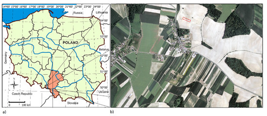
Figure 1.
(a) Location of the investigation sites; (b) location of point borders.
3. Source of DEMs
As noted above, three methods were used to obtain geospatial data:
- Method I, Figure 2a—point cloud generated based on aerial photographs;
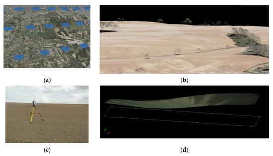 Figure 2. Analysed fragments of point clouds from: (a) aerial photographs, (b) aerial laser scanning, (c) Terrestrial Laser Scanning (TLS), (d) part of point cloud from TLS.
 - Method II, Figure 2b—aerial laser scanner point cloud; and
- Method III, Figure 2c,d—terrestrial laser scanner point cloud.
Point clouds originating from various sources have various degrees of accuracy, but they have a common georeference, which makes it possible to carry out comparative analyses of the efficacy of their use. As reference data, the point cloud generated from Terrestrial Laser Scanning (TLS) had the highest precision and the greatest point cloud density.
3.1. Aerial Photographs (APs)
The point cloud from aerial photographs was generated using the SfM (Structure from Motion) method. Stereoscopic photographs of a given area were obtained from the Store of Institute of Geodesy and Cartography, Warsaw, Poland [58]. To orient the project and fit it into the National System of Geodetic Coordinates, PUWG 1992 (EPSG-2180), coordinates of photo points located in the area during photogrammetric flight were used. The photographs were assembled through the aerotriangulation process available in the Agisoft PhotoScan Professional program with 0.15 m accuracy. The margin of error, the size of field pixels, and remaining errors resulting from the fact that the point cloud was obtained using derivative information provided by photographs, should be added to the results as well.
3.2. Aerial Laser Scans (ALSs)
A point cloud was generated from aerial laser scans obtained from the Store of Institute of Geodesy and Cartography, Warsaw, Poland [58]. Data were obtained in the format *.las, with a resolution of 4–6 points per m2. Mean error of point height determinations amounted to 0.1 m. The situational accuracy of determination of coordinates values X, Y, and Z was about 0.2 m. Data were located in the National Coordinate System, PUWG 1992 (EPSG-2180).
3.3. Terrestrial Laser Scans (TLSs)
Measurements were carried out with a terrestrial laser scanner (TLS) Leica P40 ScanStation. Accuracy of the device is stated as: range accuracy 1.2 mm + 10 ppm over its full range, with an angular accuracy of 8” horizontal, 8” vertical, which enables it to obtain results for 6 mm to 100 m heights. The device calibration process is carried out under laboratory conditions. In the field, measurements were carried out at a scanning resolution of 2 mm/10 m—i.e., at a distance of 10 m from the scanner, points are recorded horizontally and vertically every 2 mm. For georeferenced registration, uniformly distributed target points on the investigated field were used, and then the GNSS-RTK measurement was carried out. The RTK measurement was carried out with an accuracy of 0.03 m. The coordinate system used was the National Coordinate System, PUWG 1992 (EPSG-2180). For location of the point cloud within the global coordinate system, the Leica Cyclone program was used. As the accuracy of the fitting was below 0.01 m, the accuracy of every point in the point cloud set was 0.03 m.
3.4. DEMs Generation
To compare the three methods used to gather data on the investigated sites, a regular 1 × 1 m network was generated. The final comparison was carried out based on 6943 points. In the analyses, aberrant points attributed to resolution differences between generated clouds were rejected (Figure 3).
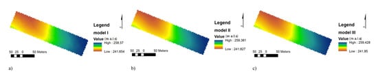
Figure 3.
DEM models of the field data generated from: (a) aerial photographs, (b) aerial laser scans, and (c) terrestrial laser scans.
3.5. LSUSLE Calculations
The L and S layers of the original equation, and LS layer later identified as the “coefficient of topography,” were calculated using a surface formulation [59] composed of unequivocally-defined coefficients produced by the selected algorithms, resulting in the digital generation of morphological features determined by hydrological slope parameters. To evaluate L, we used the ArcToolbox–Spatial Analyst Tools–Hydrology modules [60] and the algorithm of Desment and Govers [31]. The raster network cell dimension is very important for any evaluation of S [61] because slope increases as the dimension of the raster cell decreases. After determining L and S, LS at various resolutions of network cells was calculated as well.
To calculate L, we used equation proposal by Desmet and Govers [31]:
where: D is the raster resolution; A(i,j) is the unit area of feeding at the entrance to cell (i,j); m is the exponent of slope length indicator,
where: β is the ratio of rill to inter-rill erosion for conditions when the soil is moderately susceptible to both rill and inter-rill erosion
and θ is the slope angle; x is the coefficient correcting the length of flow path through raster cell, depending on flow direction and calculated based on exposure; L is the slope length coefficient (L) factor; 22.13 is the USLE unit plot length; and λ is the cumulative slope length in meters [26].
The first step in the generation of L was the evaluation of slope linear length. To this end, based on the DEMs, the layers of flow direction and flow accumulation were determined. Initially, we generated a network of direction using the one-way punctual model of flow, D8 (Figure 4). Calculations were carried out according to the equation proposed by Wilson and Gallant [62]:
where: Z is the number of adjacent cells; h is the resolution of the GRID model; h∅ (i) is distance between cell centers—1 for those located in cardinal directions (N, E, S, W)—and square root of 2 for the remaining directions.
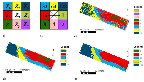
Figure 4.
Compacts of numeration of DEMs: (a) the standard system of cells, (b) coding directions of flow by the D8 algorithms [62], (c) map of flow direction, D8, Method I, APs, (d) map of flow direction, D8, Method II, ALSs, (e) map of flow direction, D8, Method III, TLSs.
The network of flow directions enabled us to determine how water flows within the area and creates a network of flow accumulation in which every following cell on the flow path accumulates water from a higher part of the area. As a consequence, a map of flow accumulation could be produced for each method (Figure 5).
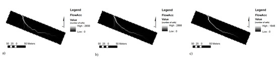
Figure 5.
Map of flow accumulation: (a) aerial photographs, (b) aerial laser scans, (c) terrestrial laser scans.
For the evaluation of the S, the McCool et al. [24,25] method was used. They found that soil loss occurs faster in slopes that were steeper than 9%. Renard et al. [18] adopted this algorithm in RUSLE for the S-factor estimation based on the slope gradient:
- S = 10.8 × sin θ + 0.03, where: slope gradient < 0.09
- S = 16.8 × sin θ − 0.5, where: slope gradient ≥ 0.09
where: θ is the gradient of slope in degrees.
Finally, we calculated the LS parameter as the product of the parameters L and S [63].
3.6. Statistical Analysis
To evaluate whether measurement data (as demonstrated by the LS parameter) had a normal distribution, we used the Kołmogorov–Smirnov test, and Statistica software, release 12. Homogeneity of measurement sequences for investigated features was checked using the non-parametric Kruskal–Wallis test [64]:
where:
and Ri is the total rank of the variables in a combined sample; ni is a random sample size; n is the sequence size; and k is the number of samples.
Comparison of L and S evaluated the techniques for taking images to generate DEMs (Methods I–III) was carried out using the linear correlation and error measures [65] listed below:
Mean error of prediction (MEP):
Root mean square error (RMSE):
Mean percentage error (MPE):
Model efficiency (ME) [66,67]:
where: is the values obtained by the TLS; are the ones obtained by ALS or AP; and n is the number of data points; is the mean value.
The relative and absolute influence of the individual elements generating the LS coefficient was evaluated by use of the ANNs of the multi-layer perceptron (MLP) type using the Statistica software, release 13.1. A total of 70% of all variables were used for the learning process; 15% were used for validation; and 15% were used to test the model. A quasi-Newton algorithm with a Broyden–Fletcher–Goldfarb–Shanno (BFGS) modification was selected for the learning of neural network. The sum of squares (SOS) was treated as the error function. Relationships between the LS parameter and model parts as independent variables were applied in all data sets. The MLP consists of three layers of neurons: input, hidden and output (it is written as m-n-p where m, n, p are numbers of perceptrons in the following layers). Each neuron had a number of inputs—from outside the network or the previous layer—and a number of outputs—leading to the subsequent layer or out of the network. The computed output response of a is based on the weighted sum of all its inputs according to an activation function [68].
4. Results and Discussion
Calculations of the LSUSLE parameter were carried out by using the original equation proposed by Desmet and Govers [31] and implemented using an automatic geological analysis (generated by ArcGIS) system, which contributed to the precision evaluation of flow accumulation. The data set of the LS coefficient was calculated using DEMs obtained from the three methods. This connected approach combining GIS software tools with DEMs of high-resolution data was used with success on regional and European scales by Panagos et al. [27].
Spatial distribution of the LS parameter and its components was determined based on DEMs generated by the ARCGIS program as presented in Figure 6.
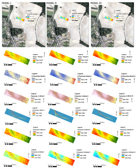
Figure 6.
Maps of parameters—S [-], L [-], slope [o], flow direction [-], flow accumulation [-], m [-] and β [-]—obtained by three methods: Model I, aerial photographs, Model II, aerial laser scans, and Model III, terrestrial laser scans.
The parameter S was between 0.06 and 4.17; the parameter β was between 0.06 and 1.89; parameter m was between 0.06 and 0.65; the parameter L was between 1.01 and 3.84; flow direction was between 1 and 128; flow accumulation was between 0 and 2868, slope was between 0.19° and 16.13°; LS was between 0.06 and 6.32 (Table 2). The lowest and at the same time the highest values were generated by means of Method I, Aerial photographs. The highest values of L were seen in Method II, Aerial laser scans. Panagos et al. [27] obtained parameters for Poland that include a mean of 0.52 and a standard deviation of 0.86; comparable values to those generated within this study, despite the significantly different DEM resolutions.
Table 2.
Statistics of Model Parameters.
Comparison of the LSUSLE models generated based on the geospatial data from the APs, ALSs, and TLSs are presented in Figure 7 and Table 3. The greatest accordance both within the DEMs and the LS parameter appeared between the ALS and TLS methods, determination coefficient R2 was 0.9992 (Figure 7C) and 0.8185 (Figure 7F) respectively. The least accordance characterized the methods AP and TLS in a case of the parameter LSUSLE R2 = 0.501 (Figure 7D).
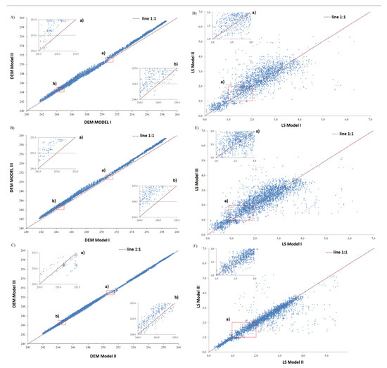
Figure 7.
Linear-regression relationship of DEMs (A–C) and LS (D–F) for the field data with AP (Model I), ALS (Model II), and TLS (Model III) methods.
Table 3.
MEP, RMSE, MPE, and ME from different DEMs and LS-factors.
ANNs were designed to validate the relative and absolute influence of the chosen parameters when evaluating the LS parameter. To this end, the MLP network type was chosen. An analysis of the quality of MLP networks should be uniformly obtained from the data sets of the LS parameter. The quasi-Newton algorithm can easily be optimized to forecast the relationship between the chosen geospatial parameters and the LSUSLE parameter. For the AP method, the activation functions were the logistic and tanh for hidden and output perceptrons, respectively; for the ALS method, the activation functions were logistic and linear, respectively; and for the TLS methods, the activation functions were tanh and exponential, respectively. Quality of learning for all three methods was extra satisfactory at 1 or near 1. Similarly, quality of testing and validating were near 1 or 1. The ANN’s learning sample error for the examined methods were 1.8 × 10⁻⁵, 5 × 10⁻⁶, and 0, respectively; for the testing sample, it was 2.4 × 10⁻⁵, 4 × 10⁻⁶, and 0, respectively; and for the validation sample, it was 1.8 × 10⁻⁵, 6 × 10⁻⁶, and 0, respectively (Table 4a,b). Analysis of the sensitivity of ANN modelling by MLP showed that geospatial parameters S and Slope had the greatest absolute influence (50.7% and 28.4%, respectively) for the AP method; parameters S and L were the greatest influence (67.2% and 11.3%, respectively) for the ALS method; and parameters S and Slope were the greatest influence (45.6% and 42%, respectively) for the TLS method (Table 5).
Table 4.
Summary of ANN analysis: (a) Fit Quality, (b) Error Measures.
Table 5.
Absolute and Relative Percentage Shares in Explaining the LS Parameter.
The LS parameter was calculated with great accuracy using high resolution DEMs. As the visual analysis of evaluated parameters (Figure 5) shows, DEM resolution influences the spatial distribution of both parameter LS and its components. High resolution DEMs reveal geomorphological changes in the ground with greater precision, and as a consequence, the evaluated values have greater accuracy. While Panagos et al. [27] carried out their analyses of erosion and particular parameters on the model of Europe, using DEMs with a 25-m resolution (earlier, 100-m resolution), the investigations we carried out show this is all possible on a smaller scale.
S, which measures the effect of slope steepness, had the greatest influence, while L influences the length of the ground slope, and in our case, L turned out to be the least essential factor in modelling the LS parameter. This can be explained by the fact that the measuring field was regular.
Flow accumulation is the total amount of water that inflows into every ground cell [69]. The traditional method of wobbulation requires repetition for the purpose of obtaining flow accumulation, what was introduced by O’Callaghan and Mark [39], as well as Tarboton [70], and is still used because of its simplicity and ease of use. However, this method is time consuming, especially in a case of vast areas, requiring substantial transformation of data [71,72,73,74,75]. Yao et al. [76] discovered an efficient method of DEM creation by sweeping various places in various ways. Su et al. [77] used the drainage-basin tree algorithm for determining how flow accumulation efficiency could be improved. Bai et al. [78] used a sequence of sorted pixels (by elevation) to collect iterations of an area of an elevation from top to bottom. Collection of flow information based on DEMs depends on flow direction, while most of the other models solve flow accumulation without regard to flow direction.
DEMs often represent of ground surface topography as a Cartesian network, triangle irregular network (TIN), or contour flow networks [79]. Regular network DEMs are convenient for calculations and conversions; the simple structure allows it to be widely used for topographic analysis and visualizations of the ground in hydrological applications [80]. Because DEMs approximate ground characteristics, the accuracy of topography, which is connected with its hydrological applications, depends on such DEM features as slope analysis, the density of river networks, flow paths, and the topographic index. DEMs used in hydrological models must be first and foremost hydrologically correct. Most DEMs contain topographic depressions, defined as areas without outlet and often called sinks and concavities [81]. In regular network DEMs, relief lowerings are areas having one or more adjacent cells which are lower than all the surrounding cells [82,83,84].
There is a strong correlation between the generalization of height data and the level of accuracy of the calculated mass of eroded material [14]. Most DEMs currently produced contain a great number of depressions that represent incorrect, false topographic errors [81,85]. The L particularly depends on the accuracy of DEMs and the precision of various calculation methods [86]. The accuracy of DEMs is also quite susceptible to horizontal resolution, vertical precision, and the density of sampling points. With the decrease of horizontal resolution, slope gradient decreases [87], and the total length of flow and density of drainage also have a decreasing tendency [88] as the concrete area of the basin increases [71]. The density of DEM sampling points on an increasing slope causes a decrease in the basin area [89,90,91]. Horizontal resolution and the density of sample points influences the total length of flow, and the slope gradient and alimentation area influence the L parameter.
The precision of transformation of the L coefficient is very sensitive to the chosen calculation methods and basic attributes that originate from DEMs, as presented above. The raster digital DEMs representing continuity of ground height above the basic level are commonly used in automatic hydrological analyses and in the generation of various basin features.
Based on the results of the LS parameter (Models I, II, and III), the A parameter (long-term average annual soil loss of the USLE model) values were calculated The particular parameters of the model (R = rainfall erosivity factor, K = soil erodibility factor, C = cropping management factors, P = conservation practices factor) were determined based on the investigations carried out for Europe by Panagos et al. [92]—parameter R; and Stone and Hilborn [93,94]—parameters: K, C, P. Regarding soil conditions and agricultural practices, values were generated for the following parameters: R = 550 MJ·mm·ha−1·h−1·yr−1, C = 0.0875 ( no-till system), P = 0.75 (cross-slope), K = 0.85 Mg·h−1·MJ−1·mm−1 (silt loam). The estimated values of the A (Mg·ha−1·yr−1) parameter were:
- Model I: 193.804, 19.328,
- Model II: 167.787, 6.934, and
- Model III 160.240,
Depending of exactness of input geospatial data, DEM from TLS and from ALS are comparable, what causes comparable results of A. This is result of character of cloud points from laser scanning, that keep geometry of objects. In a case when AP was used and point cloud was generated based on the pictures, the highest values of the parameter were obtained, what is result of use of cloud, being derivative of pictures and many treatments and processes of input data adaptation. Use of various types of input data can cause changes even up to 20%.
The obtained results were worked out using the values of R, K, C, and P and incorporating the existing conditions and variability of the LS parameter and the results of various exactness of source materials analyses for the geospatial data.
The obtained results can be extrapolated for slopes and total catchments, but the extensions are subject to limitations and problems, such as: technical and logistic restrictions on equipment, cost of equipment, and accessibility of devices and applications. Attention should be paid to the scale of the area being examined to choose the optimum measurement techniques. Exactness and precision of measurement are generally hampered as the area of investigation grows. Model precision is a derivative of the technology used and the nature of the geospatial data collected; exactness directly influences the quality of the DEM models generated.
Along with the source of data coming from the direct field measurements using AP, ALS, and TLS, additional data sources may be available like: SRTM and ASTER data and other satellite images (i.e., materials from Landstat, Modis, Sentinel 1, and Sentinel 2) for construction of digital elevation models. Taking into account the lower resolution, such data may useful in large-scale global applications, for example by regions or country or continent, but it is not recommended as a substitute for local scale (field data).
5. Conclusions
We presented DEMs and LS under the USLE model generated using three popular methods of data collection used in environmental investigations, AP, ALS, and TLS. The results of parameters generated by each method were compared. We confirmed that the highest influence shaping the LS parameter was the S parameter (index of ground slope). Additionally, we concluded that in investigations over vast areas, terrestrial laser scanners are not optimal due to the additional labor and time consumption they require. We further established that measurements sometimes cannot be carried out via TLS because ground obstacles the limit the practical extent of laser work.
In our opinion, aerial photographs or clouds of points from an aerial laser scanner are most suitable in such situations. The data generated from these methods turned out to be highly precise (comparable with the terrestrial laser scanner data). However, these methods were compared over a small area, without plant cover and without ground obstacles such as balks, reducing the uncertainty of measurement for the scope of this project. To assess the accuracy of the other two methods, the DEM and the LS parameter generated by means of the terrestrial laser scanner were taken as base or reference values because of their potentially higher accuracy.
We investigated the influence of various parameters on the LS coefficient having topological connections (connected with relief) and compared results from the terrestrial laser scanner with results from the two other methods. In spite of the fact that terrestrial laser scanner had the lowest error measure values of (that is, it was the most accurate method), we think this method has faults—such as costs and time of obtaining and transforming and the time needed for scanning of ground—when compared with the other methods. TLS may be most successful in micro applications evaluating various environmental parameters; for macro purposes, aerial laser scanners and aerial photographs are considerably quicker and cheaper, and at the same time have low error measures. Of these two methods, we believe the aerial laser scanner is most preferred.
Author Contributions
Conceptualization, E.K., P.K., M.R. and K.O.; data curation, E.K. and P.K.; formal analysis, E.K., P.K. and M.R.; investigation, E.K., P.K. and M.R.; methodology, E.K., P.K., M.R. and K.O.; project administration, E.K. and P.K.; resources, E.K., P.K., M.R. and K.O.; software, E.K., P.K. and M.R.; supervision, M.R. and K.O.; validation, E.K., P.K. and M.R.; visualization, E.K. and P.K.; writing—original draft, E.K., P.K. and M.R.; writing—review & editing, E.K., P.K. and M.R.; All authors have read and agreed to the published version of the manuscript.
Funding
The research was financed by the Ministry of Science and Higher Education of the Republic of Poland (projects nb: 2322/KG/2018, and 2315/KMiKŚ/2018).
Acknowledgments
We sincerely thank to the Agriculture-Industrial Enterprise AGROMAX Ltd. in Racibórz, Poland, for providing the experimental farmland for this study and logistic services.
Conflicts of Interest
The authors declare no conflict of interest.
References
- Ballabio, C.; Borrelli, P.; Spinoni, J.; Meusburger, K.; Michaelides, S.; Beguería, S.; Klik, A.; Petan, S.; Janeček, M.; Olsen, P.; et al. Mapping monthly rainfall erosivity in Europe. Sci. Total. Environ. 2017, 579, 1298–1315. [Google Scholar] [CrossRef]
- Ryczek, M.; Boroń, K.; Klatka, S.; Kruk, E. Wykorzystanie technik GIS do oceny zagrożenia erozją wodną na przykładzie rolniczej zlewni potoku Mątny w Beskidzie Wyspowym. Zesz. Nauk. Uniw. Przyr. Wroc. Rol. 2010, 96, 163–174. (In Polish) [Google Scholar]
- Halecki, W.; Kruk, E.; Ryczek, M. Evaluation of soil erosion in the Mątny stream catchment in the West Carpathians using the G2 model. Catena 2018, 164, 116–124. [Google Scholar] [CrossRef]
- Halecki, W.; Kruk, E.; Ryczek, M. Influence of various use scenarios on soil loss in the Mątny stream catchment in the Gorce, West Carpathians region. Land Use Policy 2018, 73, 363–372. [Google Scholar] [CrossRef]
- Shi, Z.; Ai, L.; Fang, N.; Zhu, H. Modeling the impacts of integrated small watershed management on soil erosion and sediment delivery: A case study in the Three Gorges Area, China. J. Hydrol. 2012, 438–439, 156–167. [Google Scholar] [CrossRef]
- Thomas, Z.; Abbott, B.W.; Troccaz, O.; Baudry, J.; Pinay, G. Proximate and ultimate controls on carbon and nutrient dynamics of small agricultural catchments. Biogeosciences 2016, 13, 1863–1875. [Google Scholar] [CrossRef]
- Karamage, F.; Zhang, C.; Ndayisaba, F.; Shao, H.; Kayiranga, A.; Sun, B.; Nahayo, L.; Nyesheja, E.M.; Tian, G. Extent of Cropland and Related Soil Erosion Risk in Rwanda. Sustainability 2016, 8, 609. [Google Scholar] [CrossRef]
- Halecki, W.; Młyński, D.; Ryczek, M.; Kruk, E.; Radecki-Pawlik, A. The application of Artificial Neural Network (ANN) to assessment of soil salinity and temperature variability in agricultural areas of a mountain catchment. Polish J. Environ. Study 2017, 6, 2545–2554. [Google Scholar] [CrossRef]
- Dabral, P.P.; Baithuri, N.; Pandey, A. Soil Erosion Assessment in a Hilly Catchment of North Eastern India Using USLE, GIS and Remote Sensing. Water Resour. Manag. 2008, 22, 1783–1798. [Google Scholar] [CrossRef]
- Bahadur, K.C.K. Mapping soil erosion susceptibility using remote sensing and GIS: A case of the Upper Nam Wa Watershed Nan Province. Thai. Environ. Geol. 2009, 57, 695–705. [Google Scholar] [CrossRef]
- Wójcik, A.; Klapa, P.; Mitka, B.; Piech, I. The use of TLS and UAV methods for measurement of the repose angle of granular materials in terrain conditions. Measurement 2019, 146, 780–791. [Google Scholar] [CrossRef]
- Mitka, B. Comparative analysis of geospatial data received by TLS and UAV technologies for the quarry. In Proceedings of the 18th International Multidisciplinary Scientific Geoconference SGEM: Photogrammetry and Remote Sensing, Albena, Bulgaria, 30 June–9 July 2018; Volume 30, pp. 57–64. [Google Scholar]
- Tompalski, P.; White, J.C.; Coops, N.C.; Wulder, M.A. Demonstrating the transferability of forest inventory attribute models derived using airborne laser scanning data. Remote Sens. Environ. 2019, 227, 110–124. [Google Scholar] [CrossRef]
- Bożek, P.; Janus, J. The Influence of Elevation Data Generalization on the Accuracy of the RUSLE Model. In Proceedings of the 2017 Baltic Geodetic Congress (BGC Geomatics), Gdansk, Poland, 22–25 June 2017; pp. 374–377. [Google Scholar]
- Bigdeli, B.; Amirkolaee, H.A.; Pahlavani, P. DTM generation from the point cloud using a progressive geodesic morphology and a modified Particle Swarm Optimization. Int. J. Remote. Sens. 2018, 39, 8450–8481. [Google Scholar] [CrossRef]
- Picu, I.A.C. Updating Geospatial Data by Creating a High Resolution Digital Surface Model. J. Appl. Eng. Sci. 2018, 8, 51–58. [Google Scholar] [CrossRef]
- Wischmeier, W.H.; Smith, D.D. Predicting Rainfall Erosion Losses—A Guide to Conservation Planning; Supersedes Agriculture Handbook No. 282; Department of Agriculture, Science and Education Administration: Washington, DC, USA, 1978; pp. 4–11.
- Renard, K.G.; Foster, G.R.; Weesies, G.A.; McCool, D.K.; Yoder, D.C. Predicting Soil Erosion by Water: A Guide to Conservation Planning with the Revised Universal Soil Loss Equation(RUSLE); Agriculture Handbook 703; US Department of Agriculture: Washington, DC, USA, 1997; pp. 1–251.
- Liu, B.Y.; Zhang, K.L.; Xie, Y. An Empirical Soil Loss Equation. In Proceedings of the 12th International SoilConservation Organization Conference, Beijing, China, 26–31 May 2002; Tsinghua Press: Beijing, China, 2002; pp. 143–149. [Google Scholar]
- Zhang, H.; Yao, Z.; Yang, Q.; Li, S.; Baartman, J.E.; Gai, L.; Yao, M.; Yang, X.; Ritsema, C.J.; Geissen, V. An integrated algorithm to evaluate flow direction and flow accumulation in flat regions of hydrologically corrected DEMs. Catena 2017, 151, 174–181. [Google Scholar] [CrossRef]
- Wilson, J.P.; Lam, C.S.; Deng, Y. Comparison of the performance of flow-routing algorithms used in GIS-based hydrologic analysis. Hydrol. Process. 2007, 21, 1026–1044. [Google Scholar] [CrossRef]
- Ligonja, P.J.; Shrestha, R.P. Soil Erosion Assessment in Kondoa Eroded Area in Tanzania using Universal Soil Loss Equation, Geographic Information Systems and Socioeconomic Approach. Land Degrad. Dev. 2013, 26, 367–379. [Google Scholar] [CrossRef]
- Van Remortel, R.; Maichle, R.; Hickey, R. Computing the LS factor for the Revised Universal Soil Loss Equation through array-based slope processing of digital elevation data using a C++ executable. Comput. Geosci. 2004, 30, 1043–1053. [Google Scholar] [CrossRef]
- McCool, D.K.; Brown, L.C.; Foster, G.R.; Mutchler, C.K.; Meyer, L.D. Revised Slope Steepness Factor for the Universal Soil Loss Equation. Trans. ASAE 1987, 30, 1387–1396. [Google Scholar] [CrossRef]
- McCool, D.K.; Foster, G.R.; Mutchler, C.K.; Meyer, L.D. Revised slope length factor for the Universal Soil Los Equation. Trans. ASAE 1989, 32, 1571–1576. [Google Scholar] [CrossRef]
- Liu, H.; Kiesel, J.; Hörmann, G.; Fohrer, N. Effects of DEM horizontal resolution and methods on calculating the slope length factor in gently rolling landscapes. Catena 2011, 87, 368–375. [Google Scholar] [CrossRef]
- Panagos, P.; Borrelli, P.; Meusburger, K. A New European Slope Length and Steepness Factor (LS-Factor) for Modeling Soil Erosion by Water. Geosciences 2015, 5, 117–126. [Google Scholar] [CrossRef]
- Moore, I.D.; Wilson, J.P. Length-slope factors for the revised universal soil loss equation: Simplified method of estimation. J. Soil Water Conserv. 1992, 47, 423–428. [Google Scholar]
- Moore, I.D.; Burch, G.J. Physical Basis of the Length-slope Factor in the Universal Soil Loss Equation. Soil Sci. Soc. Am. J. 1986, 50, 1294–1298. [Google Scholar] [CrossRef]
- Griffin, M.L.; Beasley, D.B.; Fletcher, J.J.; Foster, G.R. Estimating soil loss on topographically nonuniform field and farm units. J. Soil Water Conserv. 1988, 43, 326–331. [Google Scholar]
- Desmet, P.J.J.; Govers, G. A GIS procedure for the automated calculation of the USLE LS factor on topographically complex landscape units. J. Soil Water Conserv. 1996, 51, 427–433. [Google Scholar]
- Mitasova, H.; Mitas, L.; Brown, W.M.; Johnson, D.M. Terrain Modeling and Soil Eorsion Simulationa for Fort Hood and Fort Polk Test Areas; Geographic Modeling and Systems Laboratory, University of Illinois at Urbana-Champaign: Champaign, IL, USA, 1999; pp. 10–11. [Google Scholar]
- Nearing, M.A. A single, continuous function for slope steepness influence on soil loss. Soil Sci. Soc. Am. J. 1997, 61, 917–919. [Google Scholar] [CrossRef]
- Winchell, M.F.; Jackson, S.H.; Wadley, A.M.; Srinivasan, R. Extension and validation of a geographic information system-based method for calculating the Revised Universal Soil Loss Equation length-slope factor for erosion risk assessments in large watersheds. J. Soil Water Conserv. 2008, 63, 105–111. [Google Scholar] [CrossRef]
- Rodriguez, J.L.G.; Suarez, M.C.G. Methodology for estimating the topographic factor LS of RUSLE3D and USPED using GIS. Geomorphology 2012, 175–176, 98–106. [Google Scholar] [CrossRef]
- Hickey, R. Slope Angle and Slope Length Solutions for GIS. Cartography 2000, 29, 1–8. [Google Scholar] [CrossRef]
- Van Remortel, R.D.; Hamilton, M.E.; Hickey, R.J. Estimating the LS Factor for RUSLE through Iterative Slope Length Processing of Digital Elevation Data within Arclnfo Grid. Cartography 2001, 30, 27–35. [Google Scholar] [CrossRef]
- Galdino, S.; Sano, E.E.; Andrade, R.G.; Grego, C.R.; Nogueira, S.F.; Bragantini, C.; Flosi, A.H.G. Large-scale Modeling of Soil Erosion with RUSLE for Conservationist Planning of Degraded Cultivated Brazilian Pastures. Land Degrad. Dev. 2015, 27, 773–784. [Google Scholar] [CrossRef]
- O’Callaghan, J.F.; Mark, D.M. The extraction of drainage networks from digital elevation data. Comp. Vis. Graph. Image Process. 1984, 28, 323–344. [Google Scholar] [CrossRef]
- Orlandini, S.; Moretti, G.; Gavioli, A. Analytical basis for determining slope lines in grid digital elevation models. Water Resour. Res. 2014, 50, 526–539. [Google Scholar] [CrossRef]
- Moore, I.D.; Burch, G.J. Modelling Erosion and Deposition: Topographic Effects. Trans. ASAE 1986, 29, 1624–1630. [Google Scholar] [CrossRef]
- Orlandini, S.; Moretti, G.; Corticelli, M.A.; Santangelo, P.E.; Capra, A.; Rivola, R.; Albertson, J.D. Evaluationof flow direction methods against field observations of overland flow dispersion. Water Resour. Res. 2012, 48, 13. [Google Scholar] [CrossRef]
- Feng, T.; Chen, H.; Polyakov, V.O.; Wang, K.; Zhang, X.; Zhang, W. Soil erosion rates in two karst peak-cluster depression basins of northwest Guangxi, China: Comparison of the RUSLE model with 137Cs measurements. Geomorphology 2016, 253, 217–224. [Google Scholar] [CrossRef]
- Beven, K. Changing ideas in hydrology—The case of physically-based models. J. Hydrol. 1989, 105, 157–172. [Google Scholar] [CrossRef]
- Jain, S.K.; Kumar, S.; Varghese, J. Estimation of Soil Erosion for a Himalayan Watershed Using GIS Technique. Water Resour. Manag. 2001, 15, 41–54. [Google Scholar] [CrossRef]
- Lee, S. Soil erosion assessment and its verification using the Universal Soil Loss Equation and Geographic Information System: A case study at Boun, Korea. Environ. Earth Sci. 2004, 45, 457–465. [Google Scholar] [CrossRef]
- Yoshino, K.; Ishioka, Y. Guidelines for soil conservation towards integrated basen managenment for sustainable development: A new approach based on the assessment of soil loss risk using remote sensing and GIS. Paddy Water Environ. 2005, 3, 235–247. [Google Scholar] [CrossRef]
- Bhattarai, R.; Dutta, D. Estimation of Soil Erosion and Sediment Yield Using GIS at Catchment Scale. Water Resour. Manag. 2006, 21, 1635–1647. [Google Scholar] [CrossRef]
- Lee, G.S.; Choi, I.H. Scaling effect for the quantification of soil loss using GIS spatial analysis. KSCE J. Civ. Eng. 2010, 14, 897–904. [Google Scholar] [CrossRef]
- Zhang, J.; DeAngelis, D.L.; Zhuang, J. GIS-Based ER-USLE Model to Predict Soil Loss in Cultivated Land; Springer: Berlin, Germany, 2011; pp. 65–80. [Google Scholar]
- Perović, V.; Životić, L.; Kadović, R.; Đorđević, A.; Jaramaz, D.; Mrvić, V.; Todorović, M. Spatial modelling of soil erosion potential in a mountainous watershed of South-eastern Serbia. Environ. Earth Sci. 2012, 68, 115–128. [Google Scholar] [CrossRef]
- Chen, Y.; Miller, J.R.; Francis, J.; Russell, G. Projected regime shift in Arctic cloud and water vapor feedbacks. Environ. Res. Lett. 2011, 6, 044007. [Google Scholar] [CrossRef]
- Mhangara, P.; Kakembo, V.; Lim, K.J. Soil erosion risk assessment of the Keiskamma catchment, South Africa using GIS and remote sensing. Environ. Earth Sci. 2011, 65, 2087–2102. [Google Scholar] [CrossRef]
- Prasannakumar, V.; Shiny, R.; Geetha, N.; Vijith, H. Spatial prediction of soil erosion risk by remote sensing, GIS and RUSLE approach: A case study of Siruvani river watershed in Attapady valley, Kerala, India. Environ. Earth Sci. 2011, 64, 965–972. [Google Scholar] [CrossRef]
- Kumar, S.; Kushwaha, S.P.S. Modelling soil erosion risk based on RUSLE-3D using GIS in a Shivalik sub-watershed. J. Earth Syst. Sci. 2013, 122, 389–398. [Google Scholar] [CrossRef]
- Saygin, S.D.; Ozcan, A.U.; Basaran, M.; Timur, O.B.; Dolarslan, M.; Yılman, F.E.; Erpul, G. The combined RUSLE/SDR approach integrated with GIS and geostatistics to estimate annual sediment flux rates in the semi-arid catchment, Turkey. Environ. Earth Sci. 2013. [Google Scholar] [CrossRef]
- Mashimbye, Z.; De Clercq, W.P.; Van Niekerk, A. An evaluation of digital elevation models (DEMs) for delineating land components. Geoderma 2014, 213, 312–319. [Google Scholar] [CrossRef]
- Available online: http://www.gugik.gov.pl/pzgik/zamow-dane (accessed on 20 September 2020).
- Moore, I.D.; Turner, A.K.; Wilson, J.P.; Jenson, S.K.; Band, L.E. GIS and land-surface-subsurface process modeling. Environ. Model. GIS 1993, 20, 196–230. [Google Scholar]
- Pilesjö, P.; Hasan, A. A Triangular Form-based Multiple Flow Algorithm to Estimate Overland Flow Distribution and Accumulation on a Digital Elevation Model. Trans. GIS 2013, 18, 108–124. [Google Scholar] [CrossRef]
- Molnár, D.K.; Julien, P.Y. Estimation of upland erosion using GIS. Comput. Geosci. 1998, 24, 183–192. [Google Scholar] [CrossRef]
- Wilson, D.J.; Gallant, J.C. Digital terrain analysis. In Terrain Analysis: Principles and Applications; Wilson, D.J., Gallant, J.C., Eds.; John Willey & Sons, INC: New York, NY, USA, 2000; pp. 1–27. [Google Scholar]
- McCool, D.K.; Foster, G.R.; Weesies, G.A. Slope Length and Steepness Factors (LS). In Agricultural Research Service (USDAARS) Handbook 703; United States Department of Agriculture: Washington, DC, USA, 1997. [Google Scholar]
- Kruskal, W.H.; Wallis, W.A. Use of ranks in one-criterion variance analysis. J. Am. Stat. Assoc. 1952, 47, 583–621. [Google Scholar] [CrossRef]
- Rahnama, M.; Barani, G.A. Application of Rainfall-runoff Models to Zard River Catchment’s. Am. J. Environ. Sci. 2005, 1, 86–89. [Google Scholar] [CrossRef]
- Nash, J.E.; Sutcliffe, J.V. River Flow forecasting through conceptual models-Part I: A discussion of principles. J. Hydrol. 1970, 10, 282–290. [Google Scholar] [CrossRef]
- Tiwari, A.K.; Risse, L.M.; Nearing, M.A. Evaluation of WEPP ant its comparison with USLE and RUSLE. Trans. ASAE 2000, 43, 1129–1135. [Google Scholar] [CrossRef]
- Dawson, C.; Abrahart, R.J.; Shamseldin, A.Y.; Wilby, R. Flood estimation at ungauged sites using artificial neural networks. J. Hydrol. 2006, 319, 391–409. [Google Scholar] [CrossRef]
- Moore, I.D.; Grayson, R.B.; Ladson, A.R. Digital terrain modelling: A review of hydrological, geomorphological, and biological applications. Hydrol. Process. 1991, 5, 3–30. [Google Scholar] [CrossRef]
- Tarboton, D.G.; Bras, R.L.; Rodriguez-Iturbe, I. On the extraction of channel networks from digital elevation data. Hydrol. Process. 1991, 5, 81–100. [Google Scholar] [CrossRef]
- Arge, L.; Chase, J.S.; Halpin, P.; Toma, L.; Vitter, J.S.; Urban, D.; Wickremesinghe, R. Efficient Flow Computation on Massive Grid Terrain Datasets. GeoInformatica 2003, 7, 283–313. [Google Scholar] [CrossRef]
- Bhowmik, A.K.; Metz, M.; Schafer, R.B. An automated, objective and open source tool for streamthreshold selection and upstream riparian corridor delineation. Environ. Model Softw. 2015, 63, 240–250. [Google Scholar] [CrossRef]
- Magalhães, S.V.G.; Andrade, M.V.A.; Franklin, W.R.; Pena, G.C. A New Method for Computing the Drainage Network Based on Raising the Level of an Ocean Surrounding the Terrain. Adv. Cartogr. GIS 2012, 391–407. [Google Scholar] [CrossRef]
- Metz, M.; Mitasova, H.; Harmon, R.S. Efficient extraction of drainage networks from massive, radar-based elevation models with least cost path search. Hydrol. Earth Syst. Sci. 2011, 15, 667–678. [Google Scholar] [CrossRef]
- Yao, Y.Z.; Shi, X. Alternatingscanningordersandcombiningalgorithms toimprove the efficiency of flow accumulation calculation. Int. J. Geogr. Inf. Sci. 2015, 29, 1214–1239. [Google Scholar] [CrossRef]
- Yao, Y.; Tao, H.; Shi, X. Multi-types weeping for improving the efficiency off low accumulation calculation. In Proceedings of the 20th International Conference on Geoinformatics (GEOINFORMATICS), Hong Kong, China, 15–17 June 2012; pp. 1–4. [Google Scholar]
- Su, C.; Yu, W.-B.; Feng, C.-J.; Yu, C.-N.; Huang, Z.-C.; Zhang, X.-C. An Efficient Algorithm for Calculating Drainage Accumulation in Digital Elevation Models Based on the Basin Tree Index. IEEE Geosci. Remote Sens. Lett. 2014, 12, 424–428. [Google Scholar] [CrossRef]
- Bai, R.; Li, T.; Huang, Y.; Li, J.; Wang, G. An efficient and comprehensive method for drainage network extraction from DEM with billions of pixels using a size-balanced binary search tree. Geomorphology 2015, 238, 56–67. [Google Scholar] [CrossRef]
- Moretti, G.; Orlandini, S. Automatic delineation of drainage basins from contour elevation data using skeleton construction techniques. Water Resour. Res. 2008, 44, 1–16. [Google Scholar] [CrossRef]
- Gallant, J.C.; Wilson, J.P. Primary Topographic Attributes, Terrain Analysis: Principles and Applications; Wilson, J.P., Gallant, J.C., Eds.; John Wiley and Sons: New York, NY, USA, 2000; pp. 51–85. [Google Scholar]
- Zandbergen, P.A. The effect of cell resolution on depressions in Digital Elevation Models. Appl. GIS 2006, 2, 04.1–04.35. [Google Scholar] [CrossRef]
- Jensen, S.K.; Domingue, J.O. Extracting topographic structure from digital elevation data for geographic information system analysis. Photogramm. Eng. Remote Sens. 1988, 54, 1593–1600. [Google Scholar]
- Zhu, D. A Comparative Study of Single and Dual Polarisation Quantitative Weather Radar in the Context of Hydrological Modelling Structure. Ph.D. Thesis, University of Bristol, Bristol, UK, 2009. [Google Scholar]
- MacMillan, R.A.; Martin, T.C.; Earle, T.J.; McNabb, D.H. Automatic analysis and classification of landforms using high resolution digital elevation data: Applications and issues. Can. J. Remote Sens. 2003, 29, 592–606. [Google Scholar] [CrossRef]
- Lindsay, J.B.; Creed, I.F. Removal of artefact depressions from digital elevation models: Towards a minimum impact approach. Hydrol. Process. 2005, 19, 3113–3126. [Google Scholar] [CrossRef]
- Thompson, J.A.; Bell, J.C.; Butler, C.A. Digital elevation model resolution: Effectson terrain attribute calculation and quantitative soil-landscape modeling. Geoderma 2001, 100, 67–89. [Google Scholar] [CrossRef]
- Zhang, W.; Montgomery, D.R. Digital elevation model grid size, landscape representation, and hydrologic simulations. Water Resour. Res. 1994, 30, 1019–1028. [Google Scholar] [CrossRef]
- Yin, Z.Y.; Wang, X. A cross-scale comparison of drainage basin characteristics derived from digital elevation models. Earth Surf. Process. Landf. 1999, 24, 557–562. [Google Scholar] [CrossRef]
- Quinn, P.; Beven, K.; Chevallier, P.; Planchon, O. The prediction of hillslope flow paths for distributed hydrological modelling using digital terrain models. Hydrol. Process. 1991, 5, 59–79. [Google Scholar] [CrossRef]
- Wolock, D.M.; Price, C.V. Effects of digital elevation model map scale and data resolution on a topography-based watershed model. Water Resour. Res. 1994, 30, 3041–3052. [Google Scholar] [CrossRef]
- Bolstad, P.V.; Stowe, T. An Evaluation of DEM Accuracy: Elevation, Slope, and Aspect. Photogram. Eng. Remote Sens. 1994, 60, 1327–1332. [Google Scholar]
- Panagos, P.; Ballabio, C.; Borrelli, P.; Meusburger, K.; Klik, A.; Rousseva, S.; Tadić, M.P.; Michaelides, S.; Hrabalíková, M.; Olsen, P.; et al. Rainfall erosivity in Europe. Sci. Total. Environ. 2015, 511, 801–814. [Google Scholar] [CrossRef]
- Stone, R.P.; Hilborn, D. Factsheet, Universal Soil Loss Equation (USLE); Ministry of Agriculture, Food and Rural Affairs: Guelph, ON, Canada, 2000.
- Available online: http://www.omafra.gov.on.ca/english/engineer/facts/12-051.htm (accessed on 20 September 2020).


Publisher’s Note: MDPI stays neutral with regard to jurisdictional claims in published maps and institutional affiliations. |
© 2020 by the authors. Licensee MDPI, Basel, Switzerland. This article is an open access article distributed under the terms and conditions of the Creative Commons Attribution (CC BY) license (http://creativecommons.org/licenses/by/4.0/).