Abstract
High-quality focusing with accurate phase-preserving is a significant and challenging step in interferometric synthetic aperture radar (InSAR) imaging. Compared with conventional frequency-based imaging algorithms, the time-domain back-projection algorithm (TDBPA) can greatly ensure the accuracy of imaging and phase-preserving by point-to-point coherent integration but suffers from huge computational complexity. In this paper, we propose an efficient InSAR imaging method, called a frequency-domain back-projection algorithm (FDBPA), to achieve high-resolution focusing and accurate phase-preserving of InSAR imaging. More specifically, FDBPA is utilized to replace the traditional point-to-point coherent integration of TDBPA with frequency-domain transform. It divides the echo spectrum into uniform grids and transforms the range compression data into the range frequency domain. Phase compensation and non-uniform Fourier transform of the underlying scene are implemented to achieve image focusing in the wavenumber domain. Then, the interferometric phase of the target scene can be preserved by accurate phase compensation of the target’s distance. FDBPA avoids the repetitive calculation of index values and point-to-point coherent integration which reduces the time complexity compared with TDBPA. The characteristics of focusing and phase-preserving of our method are analyzed via simulations and experiments. The results demonstrate the efficiency and high-quality imaging of the FDBPA method. It can improve the imaging efficiency by more than three times, while keeping similar imaging accuracy compared with TDBPA.
1. Introduction
Synthetic aperture radar (SAR) [1,2,3,4,5,6] is a breakthrough in the field of modern remote-sensing science. It replaces the wave-front spatial sampling set obtained by the real array antenna with the echo time sampling sequence received by the synthetic array element at different spatial locations. In recent decades, SAR has demonstrated significant applications in terrain mapping, natural resource exploration, and target tracking field due to its strong transmission, all-weather, and all-day features. Interferometric synthetic aperture radar (InSAR) [7,8,9,10,11] is developed on the basis of SAR technology to higher imaging dimensions. Combining the phase information and geometric relationship of two or more pairs of SAR images relative to the same scene, InSAR can acquire a high-resolution Digital Elevation Model (DEM) and an orthophoto map of a large area. Hence, InSAR has become an effective and important remote-sensing technology for a large rolling terrain, and it is of great significance to terrain mapping, natural disaster monitoring, and resource investigation. High-precision measurement and sensing is not only one of the inevitable trend in the future development of InSAR technology but also an urgent need in the current InSAR applications. In recent years, more and more high-precision space-borne InSAR satellite systems that are developed for terrain observation, such as ALOS2 PalSAR satellite [12], Cosmo-Skymed system [13], TerraSAR/TanDEM-X binary system [14], and RCM satellite constellation [15], have been successfully launched and operated. These satellites make a great contribution to the management and exploration of the geological environment and other issues on a global scale by InSAR technology.
Serval types of algorithms based on conventional SAR image formation have been developed in the past few decades. Generally, these algorithms can be divided into two categories: one is the frequency-domain-based algorithm, e.g., range-Doppler algorithm (RDA) [16,17,18,19], chirp scaling algorithm (CSA) [20], wavenumber-domain algorithm (WKA) [21,22,23,24,25]. Another is the time-domain-based algorithm, such as the matched filter algorithm (MFA) and the back-projection algorithm (BPA) [26,27,28,29]. Classical frequency-domain algorithms are limited in their precision due to processor approximations, e.g., the platform is moving uniformly in a straight line or the reference focusing function is the same in all areas of the underlying scene. In practice, these assumptions are not always true, such as the reference focusing function will cause defocusing and phase errors of the area which are far from the reference scene center. Hence, to improve the focusing quality of InSAR, error compensation is necessary for these frequency-domain-based algorithms. Usually, the compensation process in these algorithms is complex and difficult to accurately. Moreover, the traditional frequency-domain-based methods are range-plane projection-based imaging, which may result in the interferometric phase wrapping and the target geometry distortion serious if the terrain is abrupt. In addition, due to the influences of airflow, obstacles, and other factors, the movement trajectory of the radar platform usually is complex and deviates greatly from the ideal trajectory in practice. It increases the difficulty of frequency-domain focusing, resulting in a decrease in imaging accuracy and phase extraction accuracy.
Different from the frequency-domain-based algorithms, time-domain back-projection algorithm (TDBPA) is more suitable for SAR high-resolution imaging in the case of the complex trajectory of the platform, because it can provide precise focusing and phase information of a large scene by point-to-point coherent integration without any assumption constrained. Making use of the trajectory positions from auxiliary measuring equipment, such as the inertial measurement unit (IMU) or global positioning system (GPS), TDBPA can compensate for the phase delay of the scene directly and avoid range migration correction in the frequency-domain-based algorithm. Furthermore, the imaging plane of TDBPA can be selected as a surface, which greatly reduced the geometric distortion and the overlaying caused by complex rugged topography. Therefore, even in the condition of non-ideal motion trajectory and complex terrain, TDBPA still performances well for high-precision focusing and interferometric phase extraction of a large scene. However, huge complexity and low efficiency is one obvious shortcoming of TDBPA, suffer from due to the point-by-point integration, which restricts its practical application [30,31,32,33]. Compared with the computational complexity of the frequency-domain algorithms for an image, the complexity of TDBPA grows as , which makes it difficult to be real-time imaging in InSAR large scene observation. To improve imaging efficiency of TDBPA, some efficient modified TDBP methods based on sub-aperture decomposition and scene segmentation, such as the fast factorized back-projection algorithm (FFBPA) [34,35,36,37,38,39], have been proposed for SAR imaging. Compared with the conventional TDBPA, FFBPA can reduce the computational complexity, but its imaging accuracy may decrease if the number of decomposed sub-aperture increased. Hence, FFBPA may not be suitable for InSAR high-resolution imaging with a complex trajectory.
To further overcome the drawback of TDBP, an efficient method via transform domain focusing, named as the frequency-domain back-projection algorithm (FDBPA) [40,41,42], is proposed for SAR efficient imaging. In Reference [40], the presented FDBPA transfers the point-to-point coherent integration of conventional TDBPA to the wavenumber domain. It samples the spectrum of the SAR echo data after range compression and projects the spectrum data into the wavenumber domain. Each frequency grid in the wavenumber domain contains the information of the whole image scene. Then the focused image can be obtained by taking inverse Fourier transform of the wavenumber transform data. Owing to the index of each frequency grid is uniform, the step of index value calculation can be performed only once. Compared to TDBPA, FDBPA has improved imaging efficiency and kept similar imaging precision. In Reference [41], the authors introduce the application of FDBPA in stepped-frequency SAR, which improves the computation efficiency and realizes the automatic spatial spectra cutting. In Reference [42], an efficient three-dimensional imaging method based on FDBPA is proposed for SAR imaging, the results also demonstrate the great improvement of imaging efficiency. However, only the efficiency and aggregation degree are analyzed in these FDBPA methods, without considering the phase retention, the topographic relief effect, and the phase derivation relationship of rugged topography. These FDBPA methods cannot be used for InSAR imaging directly. Moreover, the theoretical proof of these FDBPA is only based on the simulation data, without the support of the experiment results of a large scene. Exploiting the advantages of FDBPA is still a challenging issue in InSAR imaging.
In this paper, inspired by the FDBPA [40], we propose an efficient imaging method to achieve high-resolution focusing and accurate phase-preserving of InSAR imaging. The proposed method adopts a non-uniform Fourier transform instead of coherent integration and uses the accurate distance between antennas and imaging spots instead of reference distance to compensate for the delayed phase. In the scheme, the antenna position information is introduced in the azimuth non-uniform Fourier transform and the fully utilized in compensating the delayed phase of the echo signal. Compared with the traditional frequency-domain InSAR imaging algorithm, the proposed algorithm introduces the antenna position information and improves the imaging and phase accuracy. Compared with the time-domain InSAR imaging algorithm, it avoids the repetitive calculation of index and improves imaging efficiency. Therefore, the proposed algorithm is adopted to SAR imaging system, the interferometry system and bistatic system with larger scene. However, due to the complex geometric relationship of bistatic system, the range from transmit-system and receive system to the target scene is calculated separately, which leads to the uniform orthogonal distribution of the frequency grid. Thus, it is necessary to improve the algorithm to process the data from the bistatic system. In this paper, the feasibility of the proposed algorithm is verified by the simulation and measured data of different airborne interferometry system.
The rest of this paper is organized as follows: The second section describes the model of InSAR imaging and the principle of TDBP. The proposed FDBPA for InSAR imaging is introduced in the third section. In the fourth section, the simulations and experiments are applied to demonstrate the effectiveness of the proposed algorithm. The fifth part analyzes the imaging characteristics of FDBPA. Finally, the conclusions and future work are illustrated in the sixth section.
2. InSAR Imaging Model
2.1. Geometric Model
The classical geometric model of InSAR imaging is shown in Figure 1. The InSAR system adopts the single input single output (SISO) working model. The coordinate of the scattering point is . and denote the coordinate of the main antenna and slave antenna at the slow time, respectively. The range between the scattering point and antennas is and . denotes the distance from the antenna to the center of the target scene. is the baseline length of the InSAR system.
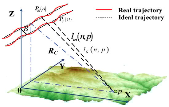
Figure 1.
Geometric model of the interferometric synthetic aperture radar (InSAR) system.
The echo signal of a target with time-delayed can be written as follows:
where is a window function, and is the scattering coefficient of target points, denotes the time-delayed of the target and , is the rectangular window function, is the center frequency of radar system, is the Doppler frequency rate, and are the pulse period in the range direction and azimuth direction, respectively, and .
2.2. TDBP Method
The basic idea of TDBP is point-to-point coherent integration and time-delayed phase compensation. Firstly, the echo data of InSAR are range-compressed by the matched filter method, which usually achieves in frequency domain. Specifically, the InSAR echo is transformed into the range frequency domain and multiplied by the reference focusing function. The signal of InSAR after range compression can be described as follows:
where , is the coordinates of the target point, denotes the ambiguity function of range direction, and is the central wavelength of the radar system.
Owing to TDBPA is not restricted by the imaging space and the echo can be projected to any plane, the suitable imaging space should be selected and divided into a grid first. For each grid point of imaging space, the range history will be calculated. According to the index value of the range cell, TDBPA projects range-compressed signal to the selected plane and simultaneously compensates the phase function from the range history. Finally, the formula of the focused signal of TDBPA can be expressed as follows:
where , and is the coordinate of the target in the selected imaging plane.
For the target point , the interferometric phase of InSAR can be written as follows:
where and ; and denotes the azimuthal time when the master and slave antennas are closest to the target scene.
Obviously, and can be accurately calculated in the TDBP algorithm, hence the high property of phase preserving can be achieved according to (5).
2.3. Problem Formation
In the conventional frequency-domain-based algorithms, the procedure of image formation mainly decomposes the two-dimensional focusing into two cascaded one-dimensional processing, furthermore, FFT is used to achieve imaging focusing in the frequency domain. Hence, its computational complexity is for an image. Although these algorithms are very fast, they are limited by several assumed conditions. E.g., if there are high-order phase compensation errors, these methods may be very difficult to accurately compensate for the error and suffer from serious defocusing.
As mentioned above, unlike frequency-domain-based algorithms, TDBPA adopts point-by-point accumulation in the spatial domain, so the accuracy of the image focusing and phase preservation can be significantly improved. According to the procedure of point-by-point accumulation, it leads to an increase in the computational complexity of TDBPA to . Obviously, for a large scene with cells, TDBPA is 2500 times slower than the frequency-domain algorithm. It seriously affects the real-time processing capability of the radar data. Although there are some fast BP imaging methods based on the improvement of methods and optimization of operation flow, e.g., FFBP method and GPU parallelization, the improvement of methods will lose precision and phase, and GPU parallelization is limited by hardware performance. Therefore, how to achieve high-efficiency, high-fidelity InSAR imaging with high precision is still a huge problem.
At present, a frequency-domain-based back-projection algorithm can not only ensure the imaging accuracy but also improve the imaging efficiency, which provides ideas for solving the problem of InSAR imaging.
3. InSAR Imaging via FDBPA
3.1. Theory
Inspired by the basic focusing theory of both frequency-domain-based algorithms and time-domain-based algorithms, FDBP adopts the idea of back projection to eliminate the azimuth and range coupling.
As mentioned above, the equation of TDBPA can be described as follows:
where and are the distance in range direction and azimuthal time in the time domain; and denotes the wavelength.
Converting (5) to the two-dimensional wavenumber domain, the formula will be converted to the following:
where is the wavenumber vector and for 2D imaging; and are the wavenumber in azimuth and range direction, respectively; is the space vector, and ; and are the distance in azimuth and range direction, respectively; and is the selected imaging space.
Equation (5) is the processing result of the conventional time-domain back-projection algorithm, (6) is the results of the wavenumber-domain back-projection algorithm. Obviously, the representations of them are very similar. Therefore, we can apply the coherent accumulation in the wavenumber domain as the equivalent of focusing imaging in the time domain.
After some rearrangements, (6) can be written as follows:
where is the distance between platform and imaging scene and , is the azimuthal velocity of the platform, is the angular frequency of the echo signal.
According to the wave theory, and are not orthogonal. Their relationship can be expressed as , where is the carrier angular frequency, and is the Doppler frequency. The central wavenumber in the azimuth direction is and , is the velocity of the radar platform, is the squint angle. It shows the coupling in azimuth and range direction. FDBPA uses the idea of back projection to realize decoupling.
Taking the back projection, (7) can be converted to the following:
where , denoting back-projection processing on . Owing to the fact that and are the uniform variables in the frequency domain and time domain, respectively, the coherent accumulation in (8) can be considered as the azimuthal non-uniform Fourier transform of .
To reflect the phase factor term in (8), the formula above also can be described as follows:
where , , is the coordinates of central point of the target scene, is the coordinates of the main antenna at slow time, in which is the slow time when the distance from platform to target scene is smallest, denotes the wavenumber-domain-focused image data, imaging result can be obtained from the 2D IFFT of . The detailed description of this conclusion has been proved in References [27,36]. contains the amplitude and phase information of the imaging scene and can be described as follows:
where and represent for the constant-coefficient relating to InSAR system parameters. Then the interference phase of FDBPA can be obtained by the following formula:
where , and and are the distance from the master and slave antenna to the imaging scene.
According to the imaging geometric relationship , in which is the length of baseline, is the antenna incident angle, is the baseline angle of inclination, The height of the target points can be calculated by the following formula:
where is the center distance, and is the phase of height obtained by after phase filtering, removing of flat earth effect, and phase unwrapping. The basic processing chain of InSAR and detailed information of phase unwrapping are introduced in References [43,44,45].
3.2. Algorithm Flow
According to the theoretical derivation above, there are mainly four steps for InSAR imaging: The first step is range compression, the second step is calculating the index, the third step is back projection, and the last one is inverse Fourier transform.
The main flow of InSAR imaging based on is demonstrated as follows (Algorithm 1):
| Algorithm 1: InSAR Imaging via FDBPA |
| Input: raw echo data and , antennas information and . Output: focused image data and . 1: Range Compressed , where is the raw echo data in the range frequency domain, is the range reference function and . 2: Calculation of Index Value a: grid division where is the sign of ceil; is the size of the target scene; and and are range and azimuth spatial resolution, respectively. b: the calculation of index value , where and are the range and azimuth frequency scaled by , respectively; and are the frequency space and starting frequency scaled by , respectively; and , . 3: Back Projection a: 1D Fourier transform b: ID extraction by Sinc-interpolation c: non-uniform Fourier Translation where denotes the non-uniform Fourier translation. d: Phase compensation , where is the distance from the center of the target point to the antenna. 4: Two-Dimensional Inverse Fourier Transform The processing step of is the same as . The interferometric phase can be obtained by the images data of and after registration. |
3.3. Phase Stability
Under the influence of an unstable imaging environment, the trajectory of the antenna platform is not an ideal linear motion. We assume the actual coordinates of radar antennas are and , respectively; and is the actual coordinates of imaging points. The error-free antenna signal of scattering point after two-dimensional focused imaging can be expressed as follows:
where denotes the range-azimuth ambiguity function of the master antenna corresponding to the target point .
Taking the RD algorithm as an example of the traditional frequency-domain algorithm, it firstly compresses the original echo signal, then corrects the distance migration in the two-dimensional frequency domain, and finally compresses the corrected echo data. The phase of the frequency-domain focusing images can be expressed as follows:
where , is the average velocity of the radar platform, and denotes the reference point, which is the center of the imaging scene.
In the proposed algorithm, the original echo data are compressed firstly. Then the data are projected into image wavenumber domain, and the non-uniform Fourier transform is implemented in the azimuth; finally, the delayed phase of the echo is compensated according to the measurement position information of antennas and scene, and the two-dimensional inverse Fourier transform is performed. Different from the traditional frequency-domain algorithm, the proposed algorithm introduces the precise antennas position information in the process of azimuth-to-Fourier transform. Secondly, the actual distance between the target points and the antennas is used instead of the reference distance when compensating for the delayed phase of the echo. Thus, the equation of the focusing scene by the proposed algorithm can be written as follows:
where denotes the coordinate of the InSAR platform obtained by the GPS and IMU of the radar system, , is the instantaneous velocity of radar platform, and for 2D imaging; is the coordinate corresponding to the target point on the imaging plane.
When antennas vibrate and deviate from the ideal antenna trajectory, the azimuth phase error of the traditional frequency-domain algorithm and the proposed algorithm can be expressed as and , respectively. The precise antenna position information obtained by high-precision positioning tools and IMU(inertial measurement units) makes the coordinate close to . Compared with , can be viewed as .
For complex terrain, the azimuth phase error of the traditional frequency-domain algorithm and the proposed algorithm can be expressed as and , respectively. FDBP-based InSAR algorithm can make use of the distance calculated by the measured antenna trajectory information and the coordinates of target points in the imaging field to compensate for the delayed phase. For non-reference points, the phase error of the RD algorithm is much larger than that of the FDBP algorithm. Thus, compared with the traditional frequency-domain algorithm, the proposed algorithm can better adapt to the complex terrain. In conclusion, compared with the traditional frequency-domain InSAR imaging algorithm, the proposed algorithm makes full use of the position information of the antenna and imaging scene, which improves phase stability, and avoids the phase error and compensation caused by the non-ideal trajectory of the antenna.
3.4. Computational Complexity
InSAR imaging algorithm based on TDBPA can be divided into two steps: the range compression and TDBPA. Their computational complexity can be described as and , respectively; and are the number of imaging cells in the azimuth direction and range direction, respectively; and is the imaging scene size.
According to the detailed algorithm flow above, the computational complexity of the proposed method consists of four parts. The computational complexity of range compression is which is consistent with the InSAR imaging algorithm based on TDBPA. The complexity of the division of spectrum grid, back projection, and 2D inverse FFT are , , and , respectively.
The main complexity of time-domain-based InSAR imaging comes from TDBPA, and the proposed algorithm suffers from the huge computational complexity mainly from back-projection. Hence, the decisive complexity of TDBPA and FDBPA are and , respectively. Obviously, FDBPA can significantly improve the computational efficiency of InSAR imaging, and the gap between the imaging efficiency of TDBPA and FDBPA becomes more obvious with the increase of scene area. It demonstrates the advantages of FDBPA in InSAR real-time imaging with large scenes.
4. Results
To verify the feasibility and effectiveness of the proposed algorithm, the simulated and actual echo data are processed by TDBP, FDBP, RD, and FFBP algorithm, respectively. In all the experiments, a computer with Intel Core i7-8700K 3.7 GHz CPU, 32 GB RAM, and NVIDIA GeForce RTX 2060 6 GB hardware capabilities, “MATLAB” programming language, CUDA 10.1, CUDNN software has been used.
4.1. Simulation Data
To compare the performance of the proposed algorithm with several classical imaging algorithms, the simulation data are processed by imaging algorithms based on TDBPA, FDBPA, RDA, and FFBPA, respectively. The main simulation parameters of InSAR are shown in Table 1. The original simulation scene is a cone with the size of . The reflection coefficient of each target point in the simulation scene is different from another according to its distance from the antenna and the unique incident angle. Figure 2a shows the simulation cone scene model. Antenna jitter is added in the trajectory and the actual trajectory is shown in Figure 2b.

Table 1.
Simulation parameters.
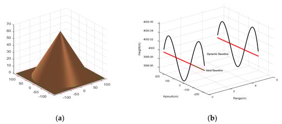
Figure 2.
Simulation scene and antennas. (a) Original cone scene. (b) The trajectories of dynamic antennas and ideal antennas.
The amplitude images and interferograms are shown in Figure 3. For comparing the results under the same situation, TDBPA and FFBPA both select the slant plane as the imaging plane. The top of Figure 3 shows the amplitude images of imaging results. Patently, all these algorithms can produce focused images well while the focused scene produced by TDBPA and FDBPA are clearer. The bottom of Figure 3 shows the interferometric images; they have the consistent distribution of interferometric fringes which demonstrates that they reflect the consistent terrain information. However, it is obvious that the interferogram obtained by the RD algorithm appears more noise points. To quantitatively evaluate the focusing effect and phase-preserving performance of FDBPA, amplitude images are evaluated by image entropy (ENT) and image sharpness (SHA) in this article, while residue, coherence (COH), signal-to-noise ratio (SNR), and sum absolute phase difference (SPD) are used to evaluate the quality of InSAR interferometric phase. Table 2 shows the detailed measurement values of the indicators above.
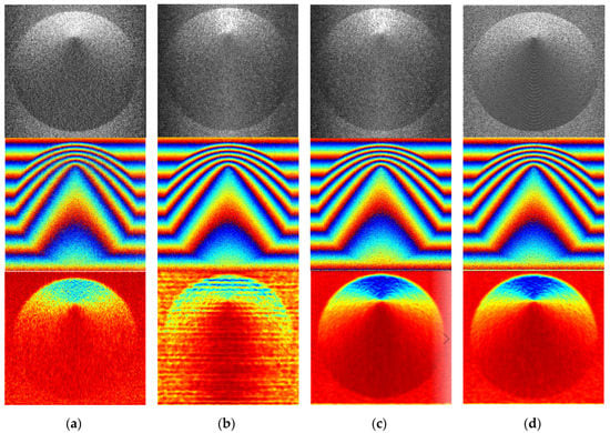
Figure 3.
The imaging results of the simulated cone: (a) range Doppler (RD), (b) fast factorized back-projection algorithm (FFBP), (c) time-domain back-projection algorithm (TDBPA), and (d) frequency-domain back-projection algorithm (FDBP) (top: amplitude, middle: interferograms, and bottom: coherence-map).
Table 2.
Quality indicators of imaging results.
ENT represents the image entropy, and the formula of ENT is as follows:
where is the probability of the occurrence of each gray level. Images entropy shows how chaotic the image is. Generally, the smaller the ENT, the better the quality of the amplitude image. However, this rule is not applicable in all cases. Especially for the experiment data, owing to the complexity of the real scene, the evaluation criteria of obtained results are not absolute. Therefore, we pay more attention to the comparison of the indicators of multiple algorithms in this paper. The formula of image sharpness can be expressed as follows:
where is the pixel value of the focused image. In contrast to ENT, the larger the value of SHA, the better quality of the image.
The residue (RES) is one of the most important indicators to represent the interference phase quality. It seriously affects the phase unwrapping in InSAR imaging processing. The definition of RES is as follows:
where denotes the wrapping phase gradient of the pixel.
SPD denotes absolute phase difference (SPD). For noiseless phases, the phase gradient of adjacent pixel points should be a relatively small value since the terrain is slowly changing. When there is noise in the phase, the phase gradient of adjacent pixels will increase sharply. Based on this principle, Li et al. proposed the sum of phase gradients (SPD). Compared with the residue based on the wrapping phase gradient, the absolute phase gradient and the absolute phase gradient are calculated based on the absolute phase, so they can more accurately reflect the denoising ability of the filtering algorithm. A detailed explain about this can be seen in Reference [46]. The equation of SPD can be written as follows:
SPD is calculated based on the absolute phase, so the quality of interferograms can be accurately reflected. In general, the small residue and SPD means the higher the quality of the interferograms, while the coherence coefficient and SNR are the opposite. The coherence (COH) between complex images is often used to measure the similarity between images and the quality of the interferograms. The coherence is defined as follows:
where is the conjugate sign, and and denote the complex image information. Moreover, the signal-to-noise ratio can be obtained by the formula .
As we can see from Table 2, all these image quality indexes of FDBPA are close to TDBPA. ENT, RES, and the value of SPD of FDBPA are slightly lower than that of TDBPA, while SHA, COH, and SNR of FDBPA are the opposite. These data demonstrate that FDBPA achieves similar imaging accuracy and phase-preserving property with TDBPA in processing the simulation data. Patently, the performances of RDA and FFBPA are closer to each other and worse than TDBPA and FDBPA. Although the ENT of RDA and FFBPA is lower than that of TDBPA and FDBPA, it is obvious that FDBPA and TDBPA have a better focusing effect according to the amplitude images in Figure 3.
To verify the imaging efficiency of FDBPA, imaging simulations under different scene sizes were implemented with imaging algorithms based on TDBPA, FDBPA, RDA, and FFBPA, respectively. The records of running time are shown in Table 3. It demonstrates that (1) FDBPA is more efficient than TDBPA when the imaging scene size is the same. It can enhance efficiency by three times at least compared with TDBPA. (2) As the increase of the target area, the advantages of FDBPA become more apparent (3) The imaging efficiency of FFBPA is similar to that of FDBPA, but with the increase of scene size, its performance is lower than that of FDBPA finally. (4) RDA has the fastest imaging speed.
Table 3.
Comparison of imaging time.
Simulations results in this chapter verify the feasibility of FDBPA in InSAR imaging. It can improve computational efficiency while keeping similar imaging accuracy and property of phase-preserving with TDBPA. It means that the InSAR imaging algorithm based on FDBPA has great application advantages and prospects.
4.2. Experiment Data
The measured data of this experiment are obtained from an airborne InSAR system based on the operation mode of single send and double receive. The airborne platform flew 5230 m above the mountainside and collects echo data of the scene. The main system parameters of InSAR are as follows: the carrier frequency, ; the signal bandwidth, ; the sampling frequency, ; the antenna aperture length, ; the pulse repetition frequency, ; the platform height, ; the radar incident angle, ; the baseline length, ; and the reference distance, . This experiment selects part of raw scene data that can reflect the imaging effect to be processed by TDBPA, FDBPA, RDA, and FFBPA, respectively.
The imaging scene is a rolling hillside. As shown in the amplitude images of Figure 4, all of these algorithms can well restore the scene, while TDBPA and FDBPA have better focus effects. Except for the slope depression, the traces of artificial mining, the trees also can be clearly distinguished in the amplitude images of Figure 4c,d. Interferograms contain terrain elevation information of the target scene. Interferograms with consistent interferometric fringes in Figure 4 show that the elevation information obtained by these used algorithms is uniform. Patently, the interferometric image of RDA has more noise points and TDBPA and FDBPA have a similar interferometric effect. Meanwhile, the interferometric image of FFBPA looks brightest and clearest because FFBPA based on sub-aperture imaging has a filtering effect on the echo data that reduces the noise points in the interference graph phase.
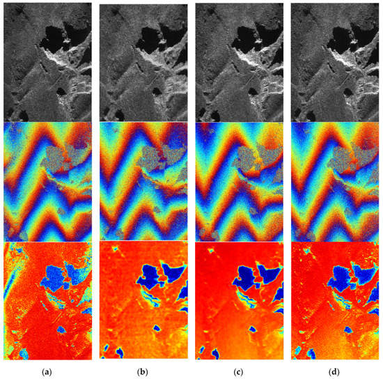
Figure 4.
The results of the experiment: (a) RD, (b) FFBP, (c) TDBP, and (d) FDBP (top: amplitude, middle: interferogram, and bottom: coherence-map).
Table 4 shows the quality indicators of Figure 4. The quality indexes of TDBPA and FDBPA are very close compared with the other two algorithms, and FDBPA performs slightly worse than TDBPA within a reasonable range which probably because of environmental noise. Furthermore, It demonstrates that the FDBPA and TDBPA have a better focusing accuracy and property of phase-preserving than RDA and FFBPA. Experiment results further prove that in practical application, FDBPA is an effective InSAR imaging algorithm. It can achieve similar imaging accuracy and the property of phase-preserving with TDBPA.
Table 4.
Comparison of quality imaging results.
Figure 5 shows the results of InSAR imaging with a farmland scene. The measured data of this experiment were obtained from an airborne InSAR system based on the operation mode of single send and double receive. The main system parameters of InSAR are as follows: the carrier frequency, ; the signal bandwidth, ; the sampling frequency, ; the antenna aperture length, ; the pulse repetition frequency, ; the platform height, ; the radar incident angle, ; the baseline length, ; and the reference distance, . This experiment selects part of raw scene data that can reflect the imaging effect to be processed by TDBPA, FDBPA, and RDA, respectively. Table 5 shows the comparison of indicators. It is clear that the imaging efficiency of FDBP is better than TDBPA, while the imaging accuracy and the phase precision are better than TDBP algorithm when processing the same data.
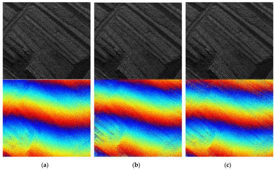
Figure 5.
The results of the experiment: (a) TDBP, (b) RD, and (c) FDBP (top: amplitude, and bottom: interferogram).
Table 5.
Comparison of quality imaging results.
Figure 6 shows the results of airborne InSAR imaging with a large scene. The radar system work in Ka-band and . The ideal imaging resolution is 0.5 × 0.5, the signal bandwidth , the imaging scene size is 4096 × 3400. The partial imaging details are shown in the highlighted red wireframe. Patently, the amplitude images of InSAR imaging algorithm based TDBP shows the best imaging effect, the amplitude image of RD-based InSAR imaging has obvious defocusing as shown in Figure 6b, while the amplitude image of InSAR imaging algorithm based FDBP shows a similar imaging effect with TDBP. The COH of interferogram in Figure 6a–c is 0.812, 0.802, and 0.809, respectively, which demonstrates the phase-preserving ability of the proposed algorithm is better than the traditional frequency-domain algorithm. InSAR algorithm based on TDBP, RD, and FDBP spent 8805.7, 37.28, and 1102.40 s, respectively, to process the airport echo data with the GPU. It shows that the proposed algorithm improves imaging efficiency, compared with TDBPA.
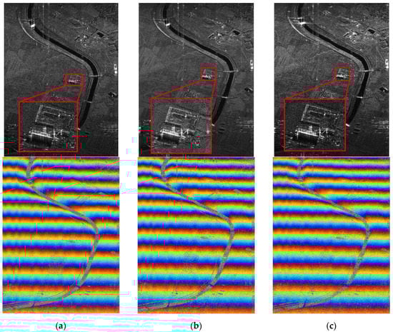
Figure 6.
InSAR imaging results of the airborne large scene. (a) TDBP, coherence (COH): 0.812, time: 8805.70 s; (b) RD, COH: 0.802, time: 37.28 s; and (c) FDBP, COH: 0.809, time: 1102.4 s (top: amplitude, and bottom: interferogram).
5. Performance Analysis
5.1. The Number of Frequency Grids
FDBPA applies back-projection ideal to the range frequency domain. Grid division is the most important step in the frequency back-projection algorithm. Different from the grid division of the time-domain back-projection algorithm, the range of the frequency-domain grid is a fixed value . Therefore, the interval of frequency grids and the number of frequency grids become important indexes to determine the imaging accuracy of FDBPA. To further explore the imaging characteristics of FDBPA, we will test the influence of these two parameters on the proposed algorithm one by one.
For testing the impact of the number of frequency grids on FDBPA, fixing the interval of grids, FDBPA with different numbers of grids are implemented to obtain the amplitude images and interferograms from the raw echo data of the simulation cone. The simulation system parameters are the same as the simulation parameters in the fourth part. The qualities of imaging results are measured by entropy, residue, coherence, absolute phase difference, and so on.
Figure 7 shows simulation results of FDBPA with the number of grid points of , , , and , respectively. Obviously, details of the cone scene in the amplitude images of Figure 7a–c are well restored, and interferometric fringes of interferograms are clear and consistent. There are similar and the change is not obvious. However, as shown in Figure 7d, the focused image is blurred seriously and the interferometric fringes become indistinct. It demonstrates when the interval of grids fixed, with the increase of grids, the scope of the spectrum search is expanded. When the scope reaches a certain level, zero-frequency information will be obtained in the echo data, causing the original scene information covered. According to (17), (18), and (19), the value of sharpness, residue, and the absolute phase difference is related to the number of frequency grids. For eliminating the impact of the change of the number of frequency grids on image evaluation indicators, 2D interpolation is carried out to fix all the focused images size to . Figure 8 shows the changing trend of ENT and RES of the focusing results.
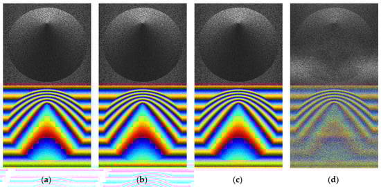
Figure 7.
The results of the simulated cone: (a) 1000 × 1000, (b) 2000 × 2000, (c) 4000 × 4000, and (d) 6000 × 6000. (Top: amplitude. Bottom: interferogram.).
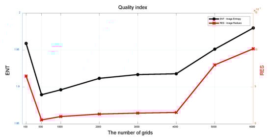
Figure 8.
Quality index of simulation data.
Table 6 is the quality evaluation of imaging results under different numbers of frequency grids. Obviously, with the increase of grids, the quality of amplitude images and interferograms continue to decrease slightly, and the value of all the indicators changes dramatically when the grids increase to . Simulation results show that FDBPA can achieve the best imaging effect with the grids calculated by the grid division equation in the third chapter, and when the imaging resolution is consistent with the InSAR system, FDBPA can obtain the best imaging results.
Table 6.
Images’ quality indicators under different grid number.
The results of measured data in Figure 9 and Figure 10, and Table 7 confirm the validity of the above conclusions. Figure 9 is the imaging results and Table 7 gives the quality indicators of images in Figure 9. Figure 10 shows the quality indicators of more control groups. Patently, the effect on image quality is minimal when the number of grids varies within a reasonable range. When the number of grids increases to , obvious noise points appear in the amplitude image, and the interferogram quality falls. Furthermore, the indicators show the best performance when the grid is which is calculated by grid division formulas with system parameters.
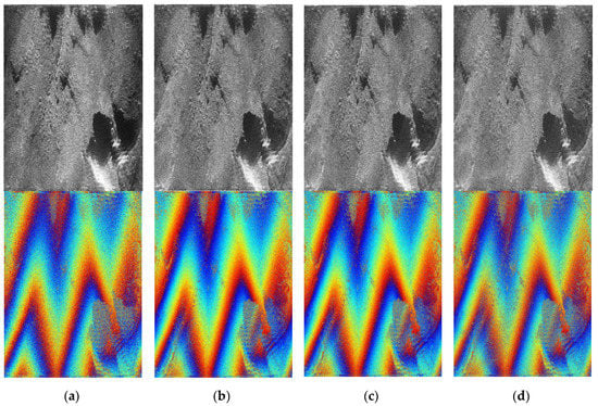
Figure 9.
The results of experiments: (a) 2000 × 2000, (b) 4000 × 4000, (c) 5000 × 5000, and (d) 7000 × 7000. (Top: amplitude. Bottom: interferogram.).
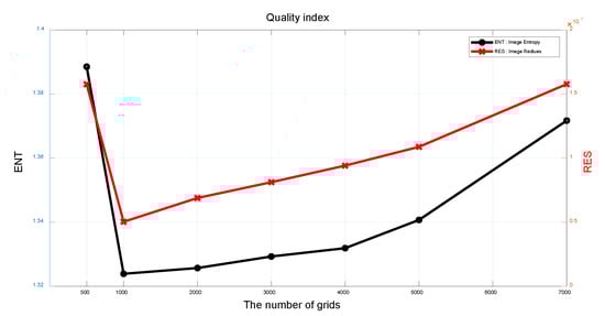
Figure 10.
Quality indicators of real-data.
Table 7.
Images’ quality indicators under different grid numbers.
5.2. The Interval of Grids
To observe the influence of the grid interval on the proposed algorithm, simulations under different intervals of grids are carried out. The remaining simulation parameters are consistent with that in the fourth section. Fixing the number of grids and observing the imaging characteristics of FDBPA with the grid interval of 0.5, 0.75, and 1.5 , respectively, where , and is the imaging scene range. According to the time-frequency-domain transformation principle, the increase of frequency interval leads to the decrease of interval in the time domain, which results in a reduction in the size of the focused images. When the value of grids interval exceeds , the target scene will be out of the range of the focused images and the phenomenon of image overlap appears. To show the imaging effect of the algorithm clearly, the amplitude images and interferometric images shown below are the part of the target scene in the focus images when the grid interval is less than .
Figure 11 is the results of the simulation data and shows the amplitude and interferometric images of the target scene. As can be seen from it that with the increase of grid interval, the target scene size increases, the details of the target scene get richer and the interference fringes in the interferograms become clearer. The main characters of the cone in Figure 11a,b, and Figure 11c are well restored and the interferometric fringes are distinct. The reduction of the proportion of the target scene in the focusing image causes the reduction of the resolution of the target scene, which also leads to the loss of the detail information of the restored images in Figure 11a,b. As shown in Figure 11d, when the grid interval exceeds , the target scene exceeds the scope of the focused image, resulting in image aliasing and image focusing failure.
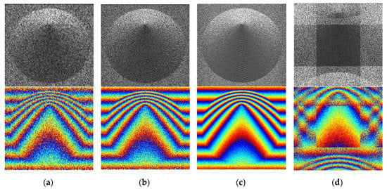
Figure 11.
The results of the simulated cone: (a) 0.5 K, (b) 0.75 K, (c) K, and (d) 1.5 K. (Top: amplitude. Bottom: interferogram.).
Similarly, Figure 12 shows only the scope of the target scene of real-data. It is clear that with the increase of grid interval within the scope of , the information of restored images increase. Figure 12d shows the restored results when the grid interval is . Patently, spectrum aliasing results in a sharp decrease in image focusing. What differs from the simulation results above is the loss of the focused images information in azimuth with the reduction of grids interval. This is because the image information on both sides of azimuth is obtained from radar half aperture data. The frequency range of the back-projection decreases with the reduction of the grid spacing, resulting in the loss of the azimuthal data of the image and the degradation of the image quality. With the shrink of grids interval, the target scene information in the azimuthal edges will get smaller until it completely disappears.
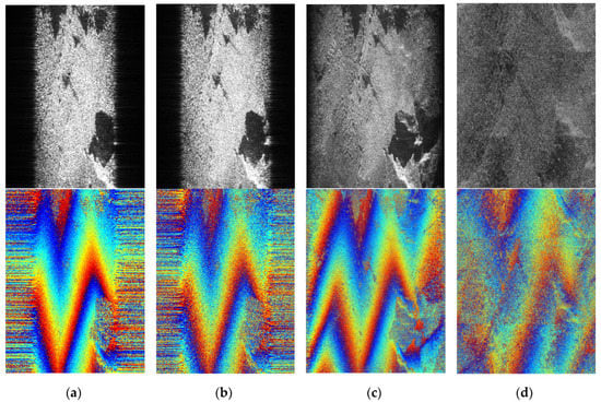
Figure 12.
The results of experiments: (a) 0.25 K, (b) 0.5 K, (c) 0.75 K, and (d) 1.5 K. (Top: amplitude. Bottom: interferogram.).
The experimental results show that the quality of amplitude images and the interference images get better with the increase of the grid interval within the range of . When the value of the grid interval exceeds , the focus image quality will decrease dramatically due to the problem of spectrum aliasing. Therefore, the optimal frequency grid interval of the proposed algorithm is .
5.3. Scene Area
The grid division formulas demonstrate that the interval of grids and the number of grids are calculated from image scene size and vary with the size of the imaging scene. Figure 13 is the target scene of imaging results with the imaging scene size is the 1, 1.5, 2, and 2.5 times of the original scene, respectively. The increase of the scene area leads to the decrease of the interval of grids and the increase of grids, while the number of imaging cells of the target scene in focused images is invariable. It is obvious that the amplitude images and interferograms are consistent with each other and have similar imaging effect under different imaging scene size. Table 8 shows the indicators of the images in Figure 13. The value of these indexes varies in a reasonable range with the increase of scene size. Figure 14 is the experiment results. The amplitude images and interferograms with different imaging scene sizes have similar effects. With the increase of the size of the imaging scene, the contour of the sunken part of the terrain from the amplitude diagram becomes clear. Correspondingly, the interferometric phase in the corresponding part of the interference image is also becoming clearer and easier to distinguish. The simulation results and actual measurement experiments prove that the enlargement of the imaging range can enrich the image details to some extent.
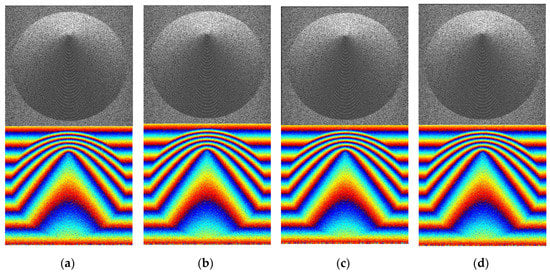
Figure 13.
The results of simulation: (a) 1 times, (b) 1.5 times, (c) 2 times, and (d) 2.5 times. (Top: amplitude. Bottom: interferogram.).
Table 8.
Images’ quality indicators under different scene size.
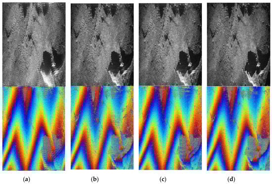
Figure 14.
The results of experiments: (a) 1 times, (b) 1.5 times, (c) 2 times, and (d) 2.5 times. (Top: amplitude. Bottom: interferogram.).
6. Conclusions
In this paper, we propose an InSAR imaging algorithm based on FDBPA with high-precision focusing and accurate phase-preserving. It applies the idea of back-projection in the frequency domain, to resolve the defocusing problem caused by range migration correction (RMC) of the traditional frequency-domain algorithm. The proposed algorithm introduces the precise antennas and scene-position information obtained from the advanced positioning system and inertial measurement unit in the imaging process. Furthermore, when compensating for the delay phase in the two-dimensional wavenumber domain, we use the real distance information from each field to the antenna, instead of the reference scene distance, which improves the focusing and phase precision and ensures the phase accuracy and stability of the proposed algorithm. The back-projection step in frequency domain avoids the repetitive calculation of the index values of the back-projection in time domain and improves the imaging efficiency on the base of the time-domain InSAR imaging algorithm. Moreover, the larger the imaging scene is, the more obvious the effect will be.
Simulation and experiment results in the fourth section primarily verify the feasibility of the proposed algorithm. The InSAR imaging algorithm based on FDBP can achieve imaging and phase accuracy similar to that of the time-domain algorithm, which is much higher than that of the frequency-domain InSAR imaging algorithm. Compared with the time-domain imaging algorithm, the proposed scheme can improve the imaging efficiency by at least three times. As the scene grows larger, its imaging efficiency advantages become more and more obvious. Results in the fifth section demonstrate that with the increase of frequency grids number, the imaging effect goes up and then down, and with the increase of grid interval, the imaging effect goes up and then down. The frequency grid number and grid spacing of the FDBP-based InSAR imaging algorithm can be calculated by the equations in calculation of index of Section 3.2, where the imaging scene size should be the same as the real measured scene size.
Author Contributions
Conceptualization, Y.W. and S.W.; methodology, Y.W. and S.W.; software, Shan Liu and J.L.; validation, Y.W. and J.L.; formal analysis, M.W.; investigation, Y.W.; resources, S.W.; data curation, Y.W.; writing—original draft preparation, Y.W.; writing—review and editing, Y.W.; visualization, S.W.; supervision, X.Z.; project administration, S.W.; funding acquisition, S.W. All authors have read and agreed to the published version of the manuscript.
Funding
This research was funded by the National Key R&D Program of China under Grant (2017-YFB0502700), National Natural Science Foundation of China (61501098, 61671113), the China Postdoctoral Science Foundation Funded Project (2015M570778), and the High Resolution Earth Observation Youth Foundation (GFZX04061502).
Conflicts of Interest
The authors declare no conflict of interest.
References
- Pi, Y.; Yang, J.; Fu, Y. (Eds.) Principles of Synthetic Aperture Radar Imaging; University of Electronic Science and Technology Press: Chengdu, China, 2007. [Google Scholar]
- Brown, W.M. Synthetic Aperture Radar. IEEE Trans. Aerosp. Electron. Syst. 1967, AES-3, 217–229. [Google Scholar] [CrossRef]
- Laurent, D.; Matthew, F.; Nicholas, M.; Poulson, J.; Ying, L. A Butterfly Algorithm for Synthetic Aperture Radar Imaging. Siam J. Imaging Sci. 2012, 5, 203–243. [Google Scholar]
- Vasco, D.W.; Rutqvist, J.; Ferretti, A.; Rucci, A.; Bellotti, F.; Dobson, P.; Oldenburg, C.; Garcia, J.; Walters, M.; Hartline, C. Monitoring deformation at the Geysers Geothermal Field, California using C-band and X-band interferometric synthetic aperture radar. Geophys. Res. Lett. 2013, 40, 2567–2572. [Google Scholar] [CrossRef]
- Mehrdad, S. Synthetic Aperture Radar Signal Processing with MATLAB Algorithms; Wiley-Interscience: Hoboken, NJ, USA, 2008. [Google Scholar]
- An, H.; Wu, J.; Sun, Z.; Yang, J. A Two-Step Nonlinear Chirp Scaling Method for Multichannel GEO Spaceborne–Airborne Bistatic SAR Spectrum Reconstructing and Focusing. IEEE Trans. Geosci. Remote Sens. 2019, 57, 3713–3728. [Google Scholar] [CrossRef]
- Wei, S.; Shi, J.; Zhang, X.; Chen, G. Millimeter-wave interferometric synthetic aperture radar data imaging based on terrain surface projection. J. Radars 2015, 4, 49–59. [Google Scholar]
- Rosen, P.A.; Hensley, S.; Joughin, I.R.; Li, F.K.; Madsen, S.N.; Rodriguez, E.; Goldstein, R.M. Synthetic aperture radar interferometry. Proc. IEEE 2000, 88, 333–382. [Google Scholar] [CrossRef]
- Yu, X.Z.; Chong, J.S.; Hong, W.; Li, Z.-J. Study on Influence of Velocity Bunching Modulation on Shallow Sea Topography Imaging by ATI-SAR. J. Astronaut. 2012, 33, 942–948. [Google Scholar]
- Wei, L.; Han, S.; Xiang, M. Processing for airborne interferometric SAR data with high squint. In Proceedings of the IEEE International Geoscience & Remote Sensing Symposium, Honolulu, HI, USA, 25–30 July 2010. [Google Scholar]
- Soumekh, M. Bistatic synthetic aperture radar inversion with application in dynamic object imaging. IEEE Trans. Signal Process. 1991, 39, 2044–2055. [Google Scholar] [CrossRef]
- Touzi, R.; Jiao, X.; Omari, K.; Sleep, B. Assessment of polarimetric PALSAR-2 potential for peatland characterization. In Proceedings of the 2016 IEEE International Geoscience and Remote Sensing Symposium (IGARSS), Beijing, China, 10–15 July 2016; pp. 3873–3876. [Google Scholar] [CrossRef]
- Serva, S.; Fiorentino, C.; Covello, F. The COSMO-SkyMed Seconda Generazione key improvements to respond to the user community needs. In Proceedings of the 2015 IEEE International Geoscience and Remote Sensing Symposium (IGARSS), Milan, Italy, 26–31 July 2015; pp. 219–222. [Google Scholar] [CrossRef]
- Floricioiu, D.; Jezek, K.; Eineder, M.; Farness, K.; Jaber, W.A.; Yague-Martinez, N. TerraSAR-X observations over the antarctic ice sheet. In Proceedings of the 2010 IEEE International Geoscience and Remote Sensing Symposium, Honolulu, HI, USA, 25–30 July 2010; pp. 2614–2617. [Google Scholar] [CrossRef]
- Komarov, A.S.; Buehner, M. Adaptive Probability Thresholding in Automated Ice and Open Water Detection From RADARSAT-2 Images. IEEE Geosci. Remote Sens. Lett. 2018, 15, 552–556. [Google Scholar] [CrossRef]
- Neo, Y.L.; Wong, F.H.; Cumming, I.G. Processing of Azimuth-Invariant Bistatic SAR Data Using the Range Doppler Algorithm. IEEE Trans. on Geosci. Remote Sens. 2008, 46, 14–21. [Google Scholar] [CrossRef]
- Bamler, R. A comparison of range-Doppler and wavenumber domain SAR focusing algorithms. IEEE Trans. Geosci. Remote Sens. 1992, 30, 706–713. [Google Scholar] [CrossRef]
- Zaugg, E.C.; Long, D.G. Generalized Frequency-Domain SAR Processing. IEEE Trans. Geosci. Remote Sens. 2009, 47, 3761–3773. [Google Scholar] [CrossRef]
- Wang, Z.; Li, Y.; Li, C.; Li, S. An Improved RD Imaging Method for SAR on Geosynchronous Orbit. In Proceedings of the 2018 China International SAR Symposium (CISS), Shanghai, China, 10–12 October 2018. [Google Scholar]
- Walker, B.; Sander, G.; Thompson, M.; Burns, B.; Fellerhoff, R.; Dubbert, D. A high-resolution, four-band SAR Testbed with real-time image formation. In Proceedings of the 1996 International Geoscience & Remote Sensing Symposium, Lincoln, NE, USA, 31 May 1996. [Google Scholar]
- Li, Z.; Liang, Y.; Xing, M.; Huai, Y.; Gao, Y.; Zeng, L.; Bao, Z. An Improved Range Model and Omega-K-Based Imaging Algorithm for High-Squint SAR with Curved Trajectory and Constant Acceleration. IEEE Geosci. Remote Sens. Lett. 2016, 13, 656–660. [Google Scholar] [CrossRef]
- Tolman, M.A. A Detailed Look at the Omega-k Algorithm for Processing Synthetic Aperture Radar Data. Master’s Thesis, Brigham Young University, Provo, UT, USA, 2008. [Google Scholar]
- Li, Z.; Wu, J.; Yi, Q.; Huang, Y.; Yang, J. An Omega-k Imaging Algorithm for Translational Variant Bistatic SAR Based on Linearization Theory. IEEE Geosci. Remote Sens. Lett. 2014, 11, 627–631. [Google Scholar]
- Milman, A.S. SAR imaging by ω—κ migration. Int. J. Remote Sens. 1993, 14, 1965–1979. [Google Scholar] [CrossRef]
- Wu, J.; Pu, W.; Huang, Y.; Yang, J.; Yang, H. Bistatic Forward-Looking SAR Focusing Using ω--k Based on Spectrum Modeling and Optimization. IEEE J. Sel. Top. Appl. Earth Obs. Remote Sens. 2018, 11, 4500–4512. [Google Scholar] [CrossRef]
- Duersch, M.I. Back projection for Synthetic Aperture Radar. Ph.D. Thesis, Brigham Young University, Provo, UT, USA, 2013. [Google Scholar]
- Duersch, M.I.; Long, D.G. Back Projection SAR Interferometry; Taylor & Francis Inc.: Abingdon, UK, 2015. [Google Scholar]
- Guo, Z.; Zhang, H.; Ye, S. Simplified and approximation autofocus back-projection algorithm for SAR. Journal Eng 2019, 20, 6408–6412. [Google Scholar] [CrossRef]
- Duersch, M.I.; Long, D.G. Analysis of time-domain back-projection for stripmap SAR. Int. J. Remote Sens. 2015, 36, 2010–2036. [Google Scholar] [CrossRef]
- Wei, S.J.; Zhang, X.L.; Shi, J.; Zou, G.-H. InSAR imaging and interferogram extraction-based the same space back-projection. Yuhang Xuebao/J. Astronaut. 2015, 36, 336–343. [Google Scholar]
- Pan, Z.; Li, D.; Liu, B.; Zhang, Q.-J. Processing of the airborne InSAR data based on the BP algorithm and the time-varying baseline. J. Electron. Inf. Technol. 2014, 36, 1585–1591. [Google Scholar]
- Yang, Y.; Pi, Y.; Li, R. Back Projection Algorithm for Spotlight Bistatic SAR Imaging. In Proceedings of the 2006 International Conference on Radar, Shanghai, China, 16–19 October 2006. [Google Scholar]
- Tan, W.; Li, D.; Hong, W. Airborne Spotlight SAR Imaging with Super High Resolution based on Back-Projection and Autofocus Algorithm. In Proceedings of the 2008 IEEE International Geoscience and Remote Sensing Symposium, Boston, MA, USA, 7–11 July 2008. [Google Scholar]
- Yegulalp, A.F. Fast backprojection algorithm for synthetic aperture radar. In Proceedings of the 1999 IEEE Radar Conference, Waltham, MA, USA, 22–22 April 1999. [Google Scholar]
- Ran, L.; Liu, Z.; Li, T.; Xie, R.; Zhang, L. An Adaptive Fast Factorized Back-Projection Algorithm With Integrated Target Detection Technique for High-Resolution and High-Squint Spotlight SAR Imagery. IEEE J. Sel. Top. Appl. Earth Obs. Remote Sens. 2017, 11, 171–183. [Google Scholar] [CrossRef]
- Liu, M.; Li, Z. A novel fast back projection algorithm based on subaperture frequency spectrum fusion in Cartesian coordinates. In Proceedings of the IGARSS IEEE International Geoscience & Remote Sensing Symposium, Beijing, China, 10–15 July 2016. [Google Scholar]
- Ulander, L.M.H.; Hellsten, H.; Stenstrom, G. Synthetic-aperture radar processing using fast factorized back-projection. IEEE Trans. Aerosp. Electron. Syst. 2003, 39, 760–776. [Google Scholar] [CrossRef]
- Ding, Y.; Munson, D.C. A fast back-projection algorithm for bistatic SAR imaging. In Proceedings of the International Conference on Image Processing, Rochester, NY, USA, 22–25 September 2002. [Google Scholar]
- Wu, J.; Li, Y.; Pu, W.; Li, Z.; Yang, J. An Effective Autofocus Method for Fast Factorized Back-Projection. IEEE Trans. Geosci. Remote Sens. 2019, 57, 6145–6154. [Google Scholar] [CrossRef]
- Li, Z.; Wang, J.; Liu, Q.H. Frequency-Domain Backprojection Algorithm for Synthetic Aperture Radar Imaging. IEEE Geosci. Remote Sens. Lett. 2015, 12, 905–909. [Google Scholar]
- Hu, K.; Zhang, X.; Shi, J.; Wei, S. A synthetic bandwidth method based on frequency-domain back projection for stepped-frequency SAR. Remote Sens. Lett. 2017, 8, 743–751. [Google Scholar] [CrossRef]
- Pu, L.; Zhang, X.; Yu, P.; Wei, S. A fast three-dimensional frequency-domain back projection imaging algorithm based on GPU. In Proceedings of the 2018 IEEE Radar Conference (RadarConf18), Oklahoma City, OK, USA, 23–27 April 2018; pp. 1173–1177. [Google Scholar]
- Bamler, R.; Hartl, P. Synthetic aperture radar interferometry. Inverse Probl. 1998, 14. [Google Scholar] [CrossRef]
- Moreira, A.; Prats-Iraola, P.; Younis, M.; Krieger, G.; Hajnsek, I.; Papathanassiou, K.P. A tutorial on synthetic aperture radar. IEEE Geosci. Remote Sens. Mag. 2013, 1, 6–43. [Google Scholar] [CrossRef]
- Yu, H.; Lan, Y.; Yuan, Z.; Xu, J.; Lee, H. Phase unwrapping in InSAR: A review. IEEE Geosci. Remote Sens. Mag. 2019, 7, 40–58. [Google Scholar] [CrossRef]
- Li, Z.; Zou, W.; Ding, X.; Chen, Y.; Liu, G. A Quantitative Measure for the Quality of INSAR Interferograms Based on Phase Differences. Photogramm. Eng. Remote Sens. 2004, 70, 1131–1137. [Google Scholar] [CrossRef]


Publisher’s Note: MDPI stays neutral with regard to jurisdictional claims in published maps and institutional affiliations. |
© 2020 by the authors. Licensee MDPI, Basel, Switzerland. This article is an open access article distributed under the terms and conditions of the Creative Commons Attribution (CC BY) license (http://creativecommons.org/licenses/by/4.0/).