Article

Global-Scale Patterns and Trends in Tropospheric NO2 Concentrations, 2005–2018

1
Department of Technology and Society, Lund University, Box 118, 221 00 Lund, Sweden
2
Golder Environmental Services, Golder Associates AB, P.O. Box 20127, 104 60 Stockholm, Sweden
3
Department of Physical Geography and Ecosystem Science, Lund University, Sölvegatan 12, SE-223 62 Lund, Sweden
4
Department of Geosciences and Natural Resource Management, University of Copenhagen, Øster Voldgade 10, DK-1350 Copenhagen, Denmark
*
Author to whom correspondence should be addressed.
Remote Sens. 2020, 12(21), 3526; https://doi.org/10.3390/rs12213526
Submission received: 9 October 2020 / Revised: 24 October 2020 / Accepted: 26 October 2020 / Published: 28 October 2020
(This article belongs to the Special Issue Air Quality Research Using Remote Sensing)

Abstract

:
Nitrogen dioxide (NO2) is an important air pollutant with both environmental and epidemiological effects. The main aim of this study is to analyze spatial patterns and temporal trends in tropospheric NO2 concentrations globally using data from the satellite-based Ozone Monitoring Instrument (OMI). Additional aims are to compare the satellite data with ground-based observations, and to find the timing and magnitude of greatest breakpoints in tropospheric NO2 concentrations for the time period 2005–2018. The OMI NO2 concentrations showed strong relationships with the ground-based observations, and inter-annual patterns were especially well reproduced. Eastern USA, Western Europe, India, China and Japan were identified as hotspot areas with high concentrations of NO2. The global average trend indicated slightly increasing NO2 concentrations (0.004 × 10¹⁵ molecules cm−2 y−1) in 2005–2018. The contribution of different regions to this global trend showed substantial regional differences. Negative trends were observed for most of Eastern USA, Western Europe, Japan and for parts of China, whereas strong, positive trends were seen in India, parts of China and in the Middle East. The years 2005 and 2007 had the highest occurrence of negative breakpoints, but the trends thereafter in general reversed, and the highest tropospheric NO2 concentrations were observed for the years 2017–2018. This indicates that the anthropogenic contribution to air pollution is still a major issue and that further actions are necessary to reduce this contribution, having a substantial impact on human and environmental health.

Graphical Abstract

1. Introduction

Air pollution is one of the main threats to human health, ecosystems and climate on a global scale [1,2]. The global population is growing substantially, and more than half of the world’s population now live in urban areas. Large urban areas and high population densities are hotspots for air pollution [1,3]. According to the World Health Organization (WHO), about 3 million people die annually due to ambient air pollution, mainly in low- and middle-income countries, and about 90% of the world’s population are exposed to air that exceeds the WHO air quality guidelines [4].
Nitrogen dioxide (NO2) is one of the most important air pollutants in the atmosphere [5] and linked to a number of both environmental and epidemiological effects [2,6]. It is formed in processes where nitrogen reacts with oxygen in high temperatures, e.g., through lightning and the combustion of fuels [7]. The main anthropogenic sources of NO2 emissions are transport, industry processes and energy production [8]. Some of the main environmental effects linked to high NO2 concentrations are acidification, eutrophication and photochemical formation of ozone (O3) [6,7,9]. NO2 also modifies the radiative balance in the atmosphere and influences the atmospheric lifetime of greenhouse gases [10,11]. NO2 is toxic at high concentrations, and the epidemiological effects include respiratory illnesses such as lung cancer, asthma exacerbations and cardiopulmonary mortality [2,5,7,12]. NO2 has a short atmospheric lifetime, on average 3.8 ± 1.0 h (mean ± 1 standard deviation) [8] as it reacts with sunlight, which triggers the production of hydroxyl radical OH [13]. Therefore, high concentrations of tropospheric NO2 are mainly confined to its emission sources, which in general are urban and industrialized areas [2,5].
Monitoring of NO2 concentrations can be done with ground-based monitoring stations. However, monitoring stations tend to be clustered in city centers, have a small spatial coverage and are often lacking in developing countries [2,14]. Ground-based air quality monitoring is thereby unevenly distributed, and large areas are under-represented [14,15]. An alternative approach to monitor air pollution is the usage of remotely sensed satellite data that increase the spatial coverage. Major advances have been made over the past decades to use satellite sensors to monitor atmospheric pollutants [1]. Satellite monitoring of NO2 started in 1995 with the Global Ozone Monitoring Experiment (GOME) instrument [3]. Since then, other satellite instruments have been used to monitor tropospheric NO2, such as GOME-2, the SCanning Imaging Absorption spectroMeter for Atmospheric CHartographY (SCIAMACHY), the Ozone Monitoring Instrument (OMI) and the recent TROPOspheric Monitoring Instrument (TROPOMI) aboard Sentinel-5 Precursor. Out of these instruments, OMI offers the longest continuous monitoring record (ongoing since 2004) and has a relatively high spatial resolution (13 × 24 km2 at nadir) [6,7]. Potential errors in estimating NO2 concentrations from satellite data include uncertainties in surface albedo, aerosols, cloud parameters, slant column density and air mass factor calculations [2,6,16]. Therefore, for satellite-based products to be trustworthy, the data need to be compared against other observations of NO2 concentrations, such as from ground-based monitoring stations [17].
Studies of long-term trends in air pollution provide information about likely changes and distribution patterns that are useful for assessing the effects of emission mitigation efforts [18,19,20]. Such studies investigating NO2 trends using OMI data and validating derived results against ground-based measurements have been performed previously. For instance, there are studies on NO2 trends over USA [2,15,21], over China [22], Russia [23], in eight European cities [1] and in cities around the globe [24]. These studies have reported declining NO2 trends in their respective study areas and relationship between OMI and ground-based measurements with correlation coefficients ranging between 0.3 and 0.93. NO2 trend studies on a global scale have also been performed previously using various satellite sensors, but these studies have overall found both negative and positive trends [3,5,19,25,26].
For trend analysis, one of the most widely used methods is the ordinary least-squares (OLS) linear regression, as performed in most of the above-mentioned studies. These simple linear models only provide partial insights on the mechanism essential for an appropriate attribution of drivers of changes. Actual changes can abruptly occur caused by climatic extreme events, anthropogenic mitigations efforts or changes in contributing factors to air pollution. These changes may only be visible for a short period in time, despite having long-lasting effects, and will therefore remain undetected using such traditional linear trend models [27,28,29].
Recent advances in time-series and breakpoint analysis open new possibilities for studying tropospheric NO2 concentrations observed by Earth observation satellites, as they allow for the detection of nonlinear trends and turning points in the concentrations. Nonlinear trend models (e.g., PolyTrend) can separate trends into linear and nonlinear trend types [30]. Piecewise linear models, such as Break For Additive Season and Trend (BFAST) [27] or Detecting Breakpoints and Estimating Segments in Trend (DBEST) [29], allow for separating time-series into individual segments, capturing dynamics in specific explanatory variables [28,31,32,33]. By using these methods, dynamics in tropospheric NO2 concentrations may be better characterized by capturing specific atmospheric conditions and stages of pollution development through time.
Hence, the main aim of this paper is to analyze global and regional patterns and trends in tropospheric NO2 concentrations using a continuous time-series of tropospheric NO2 concentrations from the OMI instrument from 2005 to 2018 with novel methods within time-series and breakpoint analyses. Specifically, we aim at (1) comparing the OMI data against NO2 concentrations from ground-based monitoring stations, (2) analyzing spatial patterns and temporal (nonlinear) trends, (3) investigating whether regional differences can be found in global NO2 concentrations and (4) spatially explicitly detecting major breakpoints in NO2 concentrations and estimating their timing and magnitude at global scale.

2. Materials and Methods

2.1. Satellite-Based NO2 Dataset

Aura is one of the National Aeronautics and Space Administration’s (NASA) Earth Observing System (EOS) satellites. It was launched in 2004 with the mission to collect data of global air pollution and to monitor the chemistry and dynamics of Earth’s atmosphere on a daily basis [34]. Aboard Aura there are four instruments, one of which is OMI [34,35]. OMI is a nadir-looking push broom hyperspectral imaging spectrometer that measures reflected solar radiation in the ultraviolet and the visible light (UV/VIS) channels of the electromagnetic spectrum (wavelength range of 264–504 nm) with a spectral resolution of 0.42–0.63 nm [36,37].
We used the OMI/Aura level 3 NO2 (OMNO2d) standard product (the cloud screened subset 4) downloaded from NASA’s Earth Observation data collection [38]. The OMNO2d product contains composites of daily total tropospheric column NO2 data with a spatial resolution of 0.25° × 0.25°. In this study, we used OMI data from 1 January 2005 until 31 December 2018 (in total, 5092 daily OMNO2d files considering 21 gaps in the daily data files). We also excluded all pixels with less than 50 days of data per year, in order to minimize influences of errors in the retrieval process.

2.2. Ground-Based NO2 Dataset

The ground-based data are annual averages (n = 6093) of daily observations of atmospheric NO2 concentrations (n = 1,706,830) from monitoring stations in the USA between the years 2005 to 2018, provided by the United States Environmental Protection Agency (US EPA) [39]. The reference method used by the US EPA for collection of ambient NO2 is chemiluminescence analysis [40] based on the reaction of nitric oxide (NO) with ozone (O3). The principle of the method is that a sample of ambient gas enters a reaction chamber where NO molecules react with O3 to form NO2. The reaction produces a quantity of light, a phenomenon known as chemiluminescence. The intensity of the light, which is proportional to the concentration of NO2, is then measured to determine the concentration of NO2 [40,41].

2.3. Comparison against Ground Observations

The daily OMI NO2 data were first averaged monthly, and thereafter annually. Annual averages were used since this study focuses on long-term trends, and it is therefore the inter-annual variability that must be validated. The annual averages were then compared to corresponding ground-based NO2 data in order to verify the validity of OMI NO2 product. Since the two datasets use different units (1015 molecules cm−2 for the satellite-based data and part per billion (ppb) for the ground-based data), we calculated z-scores using the z-statistic ((data value − average)/standard deviation) for both datasets. The relationships between the two datasets were quantified using the root-mean-square error (RMSE), and by goodness-of-fit when fitting the ordinary least-squares linear regression on the z-scores for the two datasets.

2.4. Analysis of Spatial Patterns and Temporal Trends

The spatial patterns were analyzed by averaging all OMI NO2 data pixel-wise over the study period. For analyzing the temporal trends, time-series of annual mean NO2 concentration were first calculated. Then we applied PolyTrend to analyze and classify trends in the annual NO2 time-series 2005–2018. We also applied the DBEST program to detect the greatest significant breakpoints in the annual NO2 time-series and estimate their timing and magnitude. The PolyTrend and DBEST analyses were both performed at pixel level having a statistical significance threshold (α) of 0.05. Pixels with an absolute value of annual average tropospheric NO2 concentration below the OMI detection limit (0.5 × 10¹⁵ molec.cm−2) [42] were excluded from the trend analyses.

2.4.1. Nonlinear Trend Analysis with PolyTrend

PolyTrend is an automated method with an algorithm that accounts for nonlinear change in a trend [30]. It uses a polynomial fitting-based scheme that divides trends into linear and nonlinear trend behaviors and then subdivides the nonlinear trends into classes of cubic, quadratic, and concealed trend types. The linear trend type means that the trend line has a uniform direction over the study period (either increasing or decreasing). The quadratic trend type is a trend line with one bend in its curve, implying that the cell has experienced one direction-change in its trend line over the study period (i.e., first positive and then negative trend, or vice versa). The cubic trend type means that the trend line has two bends, implying that corresponding cell has experienced more than one change in the trend direction over the study period (i.e., first decreasing followed by increasing and then again decreasing change, or vice versa). The concealed trend type consists of cells with either cubic or quadratic trend types, but with no significant net change in tropospheric NO2 concentrations over the study period. We refer to Jamali et al. [30] for more details.

2.4.2. Breakpoint Analysis with DBEST

DBEST was developed for analyzing time-series of satellite sensor data, and it uses a segmentation method for two main algorithms of trend generalization and change detection [29]. We used its change detection algorithm in order to detect breakpoints with greatest change in tropospheric NO2 concentrations. Our input data in DBEST were the pixel-wise time-series of the annual average NO2 concentrations data.
First, DBEST tests for the occurrence of discontinuities, in this case of tropospheric NO2 concentrations, by analyzing the absolute differences between consecutive data points and comparing this to the first level-shift-threshold set by the user (Table 1). If the difference is greater than the first level-shift-threshold, then it tests whether or not this difference caused a significant shift in the mean level of tropospheric NO2 concentrations and persisted over the duration-threshold. If the mean level before and after this identified discontinuity is greater than the second level-shift-threshold, DBEST considers this a level-shift point. DBEST then repeats this process for all data points, sorts them into descending order based on the absolute value of tropospheric NO2 concentrations difference, and tests if the spacing between a data point and an identified level-shift point is at least the duration-threshold. The trend component of the time-series is then segmented using a peak/valley detector function and a method that draws a straight line through detected peak/valley points and compares perpendicular distances to the non-peak and non-valley points between them with the distance-threshold parameter. If the distance is greater than this threshold, these points are added to the set of detected peak/valley points and level-shift points, all of which are called turning points. Detected turning points are then fit to the tropospheric NO2 concentrations trend using piecewise linear modelling, and those turning points that minimize the Bayesian Information Criterion (BIC) [43] are considered breakpoints. Here, we used the change detection algorithm of DBEST with a set value (2) for the number of significant breakpoints of interest for detection (Table 1), and as such, DBEST identifies a final set of greatest significant breakpoints as requested by user. The results of the change detection algorithm include the starting time of the breakpoints (break date); the change duration, or the temporal period over which this change occurred; the change value, or the amount of change that occurred over this time period; the change type, whether the change is abrupt (level-shift) or non-abrupt; the change significance, based on the statistical significance level (α = 0.05).
Here, the annual average tropospheric NO2 concentrations time-series data were set as non-cyclical type (Table 1). The first level-shift-threshold was set to 0.1 × 10¹⁵ molecules cm−2 and the second level-shift-threshold to 0.5 × 10¹⁵ molecules cm-2. It is recommended that the first level-shift-threshold be set to a smaller value than that for the second level-shift-threshold [29]. Therefore, if a detected change was quick (between two consecutive observations/years) and large enough (0.1 × 10¹⁵ molecules cm−2) to shift the mean over the user-set duration (2 years) by 0.5 × 10¹⁵ molecules cm−2 before and after the point, it was characterized as an abrupt change, otherwise it was considered a non-abrupt change, provided that it was a significant breakpoint. The distance-threshold is normally set to be a default that is derived internally by DBEST.

3. Results

3.1. Data Comparison against Ground Observations

The comparison of OMI data against ground-based observations showed a strong relationship (Pearson’s correlation coefficient R = 0.65) that was statistically significant (p-value < 0.01) (Figure 1). The relationship was equally strong (R = 0.65) when separating the analysis into a comparison of how well OMI captured the spatial variability (data averaged site-wise; Figure 1b). The OMI data were most successful at reproducing the inter-annual variability (data averaged annually), for which the observations were in a very close relationship with the ground-based observations (R = 0.99) (Figure 1c). The ordinary least-squares linear trend in annual averages of the z-scores in OMI NO2 concentrations (−0.220 ± 0.027 z-scores y−1; R2 = 0.85) was very similar to the corresponding trend in the ground-based NO2 concentrations (−0.218 ± 0.022 z-scores y−1; R2 = 0.83).

3.2. Spatial Patterns

There is a distinct difference in the NO2 concentration distribution between the northern and southern hemispheres, where the higher concentrations are almost exclusively found in the northern hemisphere (Figure 2a). The primary hotspot areas are USA (Figure 2b), Western Europe (Figure 2c), and India, China and Japan (Figure 2d). While the mean global NO2 concentration was 0.2 × 10¹⁵ molecules cm−2, The Netherlands, Belgium, Germany, France, UK, Italy and Spain had the highest average NO2 concentration (on average 1.91 × 10¹⁵ molecules cm−2), followed by Japan (0.91 × 10¹⁵ molecules cm−2), India (0.43 × 10¹⁵ molecules cm−2), USA (0.38 × 10¹⁵ molecules cm−2) and China (0.36 × 10¹⁵ molecules cm−2) (Table 2). The maximum NO2 concentration was for China (28.24 × 10¹⁵ molecules cm−2) followed by Japan (14.28 × 10¹⁵ molecules cm−2), Italy (11.84 × 10¹⁵ molecules cm−2), Germany (11.34 × 10¹⁵ molecules cm−2), USA (11.25 × 10¹⁵ molecules cm−2) and India (9.22 × 10¹⁵ molecules cm−2). Due to their high concentrations in tropospheric NO2, we selected these areas as focus areas used for further analysis in the remaining part of the study.

3.3. Temporal Trends

Significant trends in NO2 concentrations were observed largely over land and to a much lower degree over oceans along boundaries with lands (Figure 3). With the insignificant no-trends masked out, 79.55% of the remaining cells had positive trend whereas 20.45% had negative trend. The increasing trends were distributed over large parts of land, but the decreasing trends were generally observed over USA (Figure 3a), Western Europe (Figure 3b), Japan and the eastern parts of China (Figure 3c). The global average trend in 2005–2018 was slightly increasing (0.004 × 10¹⁵ molecules cm−2 y−1); however, the regional negative trends were strong enough to compensate for the global rising trend of NO2 concentrations over larger areas. Globally, the strongest negative trend was −0.969 × 10¹⁵ molecules cm−2 y−1 while the strongest positive trend was only 0.363 × 10¹⁵ molecules cm−2 y−1 (Table 2).
Areas with high average NO2 concentrations, except India and western parts of China (Figure 2), generally showed negative trends (Figure 3; Table 2). On average, the strongest negative trends were found in Europe (Belgium: −0.143 × 10¹⁵ molecules cm−2 y−1; Netherlands: −0.132 × 10¹⁵ molecules cm−2 y−1; U.K.: −0.089 × 10¹⁵ molecules cm−2 y−1; Italy: −0.070 × 10¹⁵ molecules cm−2 y−1) followed by Japan (−0.049 × 10¹⁵ molecules cm−2 y−1) and USA (−0.033 × 10¹⁵ molecules cm−2 y−1). The average trend was positive over India and the Middle East. The strongest positive average trend (0.040 × 10¹⁵ molecules cm−2 y−1) was for India. Although the strongest negative trend in the focus areas (−0.946 × 10¹⁵ molecules cm−2 y−1) was for China, the average trend for the entire country was just slightly increasing (0.014 × 10¹⁵ molecules cm−2 y−1) because strong increasing trends (0.363 × 10¹⁵ molecules cm−2 y−1) were observed over large parts of the country as well (Figure 3c).

3.3.1. Trend Types

In a global context, the linear trend was the dominant trend type with a spatial coverage of 61.98%, out of which 54.47% were positive and 7.51% negative (Figure 4a, Table 3). The concealed trend was the second trend type with 21.89% spatial coverage and mainly found over east of China and Southwestern Europe (Figure 4c,d). For the remaining trends, 9.77% were quadratic and 6.36% were cubic, out of which the majority was found over the eastern parts of USA (Figure 4a) and west of Europe (Spain and Portugal) (Figure 4b,c). In the focus areas, the dominant trend type was different for different areas. In the USA, the nonlinear trends (67.59%) were spatially more than the linear trends (32.41%) (Figure 4a, Table 3). In the focus areas in Europe, the most common trend type was linear (negative), except for Spain where the nonlinear trends, particularly the quadratic negative trends (57.96%), were dominant (Figure 4c, Table 3). The most common trend type over India was linear (increasing) (84.36%), and over Japan was linear (decreasing) (43.03%). China was the country with the largest proportion of nonlinear concealed trends in NO2 concentration (45.81%); it was also the second country with the highest proportion of linearly increasing trends (39.19%) after India (84.36%) (Figure 4c,d, Table 3).

3.3.2. Breakpoints in Tropospheric NO2 Concentrations

The global tropospheric NO2 concentrations showed a slightly decreasing trend from 2005 to 2008, followed by a small, positive change (0.03 × 10¹⁵ molecules cm−2) starting in 2008, and then a gradual increasing trend between 2011 and 2018 (Figure 5a). The annual average reached its highest values towards the end of the period in 2017–2018 (0.66 × 10¹⁵ and 0.67 × 10¹⁵ molecules cm−2). Among the focus areas, only India showed a similar trend behavior but at a higher NO2 level and with a much greater positive change (0.20 × 10¹⁵ molecules cm−2) in 2015 (Figure 5d). Japan was also similar in showing a linear long-term trend with only one breakpoint change but different in that the detected breakpoint was a great negative change (−0.47 × 10¹⁵ molecules cm−2), thus resulting in an overall decreasing trend (Figure 5f). In contrast, the number of the greatest changes detected in NO2 concentrations over USA, Europe and China was two. The two greatest changes of USA (−0.50 × 10¹⁵ molecules cm−2 and −0.08 × 10¹⁵ molecules cm−2) as well as Europe (−0.08 × 10¹⁵ molecules cm−2 and −0.16 × 10¹⁵ molecules cm−2) were both negative and started either in the beginning (2004–2005) or towards the end of the studied period (2013–2016) (Figure 5b,c). The first greatest change detected over China was positive (0.78 × 10¹⁵ molecules cm−2) and started in 2008, but then a second big reverse change (−0.81 × 10¹⁵ molecules cm−2) happened in 2011 (Figure 5e). These two almost equally big but opposite changes (upward and then downward) with no relax time in between caused the overall NO2 trend being insignificant with no net-change in NO2 concentrations throughout the time period over China. This type of significant nonlinear trend was identified as concealed trend type (Figure 5e).
Figure 6a shows the greatest breakpoint change detected in the annual average NO2 concentrations at pixel level. The spatial patterns of the detected short-term changes were similar to the long-term overall trends observed over lands (Figure 3): positive breakpoints were found over large areas in all continents (79.4%) and negative breakpoints mainly over the focus areas (20.6%). The greatest negative drop was for China (−12.41 × 10¹⁵ molecules cm−2), followed by USA (−5.60 × 10¹⁵ molecules cm−2), Italy (−3.81 × 10¹⁵ molecules cm−2) and Japan (−3.78 × 10¹⁵ molecules cm−2) and then the other focus countries in Europe (Figure 6a, Table 4). The greatest positive change was also for China (6.65 × 10¹⁵ molecules cm−2) followed by India (2.13 × 10¹⁵ molecules cm−2). Range of the change values was therefore the highest for China (19.06 × 10¹⁵ molecules cm−2) and the least for Netherlands (1.59 × 10¹⁵ molecules cm−2) and Belgium (1.75 × 10¹⁵ molecules cm−2), where the average changes were high and no positive change was detected at all (Table 4). The type of majority of the detected greatest changes was non-abrupt, indicating that most of the changes occurred gradually over time, except for Belgium where the changes mainly happened abruptly (56.86%).
The starting time of the major drops in tropospheric NO2 concentrations is most often detected during the period of 2005–2009 for USA (89.6% of cells), Japan (78.8%) and Europe (57.8%) (Figure 6b). For India, the greatest positive change started most often during 2015–2017 (41.1% of cells). For China, the biggest positive change started mostly during 2008–2010 (54.3%) and then the greatest drop happened during 2011–2014 (88.7%).
In a global context, the years 2005 and 2007 were by far the years with the highest occurrence of negative breakpoints (27.7% and 17.4% respectively), indicating a major event during this period that had global effects and particularly in the focus areas (Figure 6a; Figure 7a). The time period with high occurrence of global positive breakpoints was 2008 to 2015, and the years 2008 and 2015 had the highest rates (12.4% and 12.2% respectively) (Figure 7b).

4. Discussion

The relationship between the satellite-based and the ground-based datasets supports previous OMI validation studies. For instance, the Pearson’s correlation coefficient R was 0.65, which is within the middle of the range (0.40–0.80) of several other studies [1,2,15,22]. The statistical comparison further indicated that OMI was more successful at estimating the temporal component than the spatial component (Figure 1b,c). This can partially be explained since the ground-based monitoring stations are focused on a certain emission source (e.g., traffic locations), whereas an OMI pixel (13 × 24 km2) covers a larger area with potential emission sources both within and downwind from the pixel [1]. The strong relationships with the ground-based observations still indicate that OMI data are useful giving spatially explicit time-series of tropospheric NO2 concentrations to study global patterns and trends.
The spatial distribution of average NO2 concentrations found in this study (Figure 2) resembles those in other studies [5,19,25,26], confirming that the focus areas are indeed the main hotspots of tropospheric NO2 concentrations globally. According to Krotkov et al. [25], the highest NO2 concentrations coincide with urban areas with high populations and industrialized regions. NO2 concentrations are generally much lower over oceans than that over land since there are no sources of NO2 emissions except for passing ships [44]. This indicates that the trends observed along offshore boundaries are possibly caused by atmospheric deposition of NO2 transported from their source by large-scale circulation [45]. According to Peters et al. [44], satellite instruments have issues with detecting trace gases over oceans because of the low NO2 concentrations often being below the detection limit of the instruments (0.5 × 10¹⁵ molecules cm−2).
The global and regional trends seen (Figure 3) generally agree with the results from previous studies. Previous studies have shown increasing trends over both India and China [5,19,25,26], where our results show increasing trends over both countries too (Figure 3). The decreasing trend with major drop in NO2 that we observed over Eastern USA confirms the previous study by Krotkov et al. [46] reporting a dramatic decrease in OMI NO2 from 2005 to 2015, as a result of both technological improvements and stricter regulation of emissions. In agreement with our trend results derived for Western Europe, recently Wang et al. [47] observed decreasing trends over Netherlands, Belgium, Germany and Italy, as detected in OMI NO2 concentrations for 2012–2018. The trend results seem to be consistent among studies with data used from different satellite instruments and/or study periods [5,19,25,26].
Decreases of NO2 concentrations can primarily be attributed to either local-, regional- or country-level environmental regulations, improvements in emission control technology (e.g., power plants and vehicles), or economic changes and the associated effects in energy usage [24,25]. Since the spatial distribution of average concentrations and significant decreasing trends correlate well, this indicates that environmental regulations and technological improvements in the countries with the most severe pollution have had a positive effect on concentrations of NO2. However, it should also be noted that the two final years of this study period (2017–2018) were the years with the highest average global concentrations. This clearly shows the importance of continuous satellite-based monitoring of global patterns and trends in NO2 concentrations, also for assessing the effects of regional environmental regulations and technological improvements to reduce emissions [48].
Linear regression models assume that changes occur linearly and gradually, which is not always the case [30,49]. Here, a polynomial fitting-based scheme (PolyTrend) was used to account for nonlinear trends. This polynomial approach thus helps to detect nonlinear trends in time-series that would not be identified by an ordinary least-squares (i.e., linear model) approach. The linear trend type was the dominant trend type globally (Figure 4; Table 3) as well as for Europe (except Spain), India and Japan, indicating monotonic (non-decreasing or non-increasing) trends over these areas. The nonlinear trends with a significant slope (quadratic and cubic) were mainly found over eastern parts of USA and Spain. Since the curve of these trends has one (quadratic) or two (cubic) bends, this indicates that the NO2 concentration trends in these areas either started with an increase and then decreased or the opposite started with a decrease and then increased (quadratic), or with even more short-term changes in the direction of the trend (cubic). The latter case is in agreement with the regional trend curve for USA: a cubic trend starting with a short-term downward trend, then an upward trend, and then again another downward trend (Figure 5b). The identified areas with the concealed trends, mainly in the eastern parts of China and south of Spain, are new findings that, up to the best of our knowledge, have not been reported yet. The reason is that the OLS method is often used in trend studies, and such nonlinear trends are not detectable when OLS is applied for the entire studied period. If OLS applies here, no significant trend in 2005–2018 is detected. However, the concealed changes are credible patterns of nonlinear changes such as the greatest breakpoint changes we detected in NO2 concentrations over China.
The majority of the detected significant breakpoints were non-abrupt indicating that the concentrations of NO2 changed gradually, possibly due to stricter environmental regulations or economic cycles, as opposed to abrupt changes (e.g., in Belgium and Netherlands), which could be due to power plants or industries that have been either opened or shut down suddenly. The years 2005 to 2009 were by far the years with the highest occurrence of negative breakpoints, and regional-scale reductions of tropospheric NO2 concentrations were also observed for USA, Europe and Japan during these years (Figure 5, Figure 6 and Figure 7). It has also previously been pointed out that 2008 was a year of significant reductions in NO2 emissions (e.g., [21,22,50,51]) due to the start of the great economic recession [50,51]. This was an event, which caused large-scale economic reductions and affected anthropogenic activity globally, which in turn reduced the associated emissions of air pollution from, for example, vehicles, power plants and industries. According to the results of this study, the largest change magnitudes in NO2 concentrations during 2005–2008 were found in USA and Japan. The European countries appear to have suffered less, based on the changes in tropospheric NO2 concentrations (Figure 6, Table 4). The negative breakpoint we found over Eastern China with a four-year duration (2011–2014) is in general agreement with Li et al.’s [52] study of analyzing global change of tropospheric NO2 from 2012 to 2017 using data from the Ozone Mapping Profiler Suite (OMPS) Nadir Mapper (NM) onboard the Suomi National Polar Partnership (SNPP). They reported a large decline of NO2 in Eastern China started in 2013 and was almost entirely driven by wintertime decreases, thus indicating a decrease in anthropogenic emissions over the area. Souri et al. [53] in their study of analyzing long-term trends of OMI NO2 concentration 2005–2014 over East Asia, also found downward trends in Japan and more developed Chinese cities such as Guangzhou and Beijing, and upward trends in the majority of northern regions of China in 2010–2013. This supports the concealed trend (upward–downward) we observed for China. Another study by Krotkov et al. [46] also showed similar severe declines of NO2 in Eastern China in 2011–2014 due to an economic shutdown and government efforts to restrain emissions from the power and industrial sectors. Likewise, the steepest increasing trend we observed was over India, and they reported a fast-growing trend from 2005 to 2015 for India’s NO2 level from coal power plants and smelters.
The time-series analysis methods used in this study (PolyTrend and DBEST) benefit from recent developments, as mentioned earlier, but like many other methods they also have weaknesses. They work on a pixel-by-pixel basis, and they consider each pixel’s time-series data as an isolated entity in their trend classification and change detection procedure; the spatial behavior of adjacent areas is not used to improve the robustness of trend/change detection [54]. Thus, the obtained trend and breakpoint results should be interpreted with caution.
Future research could include multiple breakpoint detection analyses using data for pre- and post-pandemic phases of COVID-19 to study impacts of possible changes in anthropogenic sources of NO2 emissions (e.g., transport, industry processes and energy production) on air pollution and tropospheric NO2 concentration trends.

5. Conclusions

This study contributes to the ongoing research regarding spatiotemporal patterns and trends in tropospheric NO2 concentrations using data from the OMI instrument, and it investigates how the tropospheric concentrations have changed globally and regionally over the period of 2005 through 2018. By applying novel techniques for analysis of time-series and their breakpoints, we quantified long-term nonlinear trends and provided information about distribution patterns in the point in time with the greatest changes.
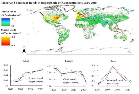
  • Globally, the tropospheric NO2 concentration showed a slightly increasing long-term trend (0.004 × 10¹⁵ molecules cm−2 y−1) for the time period 2005–2018. A significant, positive change (0.03 × 10¹⁵ molecules cm−2) was observed during 2008–2011.
  • Over Eastern USA, we found a negative trend of NO2 concentration (−0.033 × 10¹⁵ molecules cm−2 y−1) with two major breakpoint changes of −0.50 × 10¹⁵ and −0.08 × 10¹⁵ molecules cm−2 during 2005–2009 and 2013–2016, respectively.
  • Over Western Europe, the annual average NO2 concentration decreased slowly (−0.008 × 10¹⁵ molecules cm−2 y−1) and in a nonlinear manner including two major drops of −0.08 × 10¹⁵ and −0.16 × 10¹⁵ molecules cm−2 during 2006–2008 and 2016–2018, respectively. Most of the breakpoints changes detected over Netherlands and Belgium were negative and of abrupt type.
  • Over India, the steepest rising long-term trend in NO2 concentration (0.040 × 10¹⁵ molecules cm−2 y−1), among the other hot spot areas, was observed, and toward the end of the study period (2015–2017) the NO2 concentration raised even at a higher rate.
  • Over China, the linear long-term trend was positive with a slight slope (0.014 × 10¹⁵ molecules cm−2 y−1). However, by using the polynomial trend method, we found a nonlinear concealed trend containing one major positive change (0.78 × 10¹⁵ molecules cm−2) during 2008–2011 and one big negative change (−0.81 × 10¹⁵ molecules cm−2) thereafter in 2011–2016.
  • Over Japan, a considerable drop in NO2 concentration (−0.47 × 10¹⁵ molecules cm−2) was observed in 2005–2009, and the long-term NO2 trend became the strongest downward trend (−0.049 × 10¹⁵ molecules cm−2 y−1) as compared to all other focus areas.
Despite the breakpoint changes detected for the focus areas, the linear trend was the dominant trend type at global scale with a spatial coverage of 61.98%, out of which 54.47% were positive and 7.51% negative. The concealed trends, mainly observed over Eastern China and South Spain, ranked second. The years 2005 and 2007 were the years with the highest occurrence of negative breakpoints (27.7% and 17.4% respectively), indicating a major event during these years that had global effects and in the focus areas in particular. However, the trend thereafter reversed, and throughout the study period, the years 2017–2018 had the highest tropospheric NO2 concentrations. This indicates that the anthropogenic contribution to air pollution is still a major issue, and that further actions are necessary to reduce this contribution. These techniques for analysis of time-series and their breakpoints could be used for studying underlying causes to regional patterns in trends, possibly providing insights to impact of environmental regulations and other actions to prevent air pollution, having substantial impact on human and environmental health.

Author Contributions

Conceptualization, T.T. and D.K.; methodology, S.J., T.T. and D.K.; software, S.J.; validation, D.K. and T.T.; formal analysis, S.J. and T.T.; investigation, S.J. and T.T.; data curation, T.T. and D.K.; writing—original draft preparation, D.K.; writing—review and editing, S.J. and T.T.; visualization, S.J., D.K., and T.T.; supervision, S.J. and T.T.; funding acquisition, T.T. All authors have read and agreed to the published version of the manuscript.

Funding

This research was funded by the Swedish National Space Board (SNSB Dnr 95/16). T.T. was also funded by the Danish Council for Independent Research (DFF, Grant ID: DFF-6111-00258).

Acknowledgments

We acknowledge NASA Goddard Space Flight Center, Goddard Earth Sciences Data and Information Service Center (GES DISC) for providing OMI/Aura NO2 Cloud-Screened Total and Tropospheric Column L3 (OMNO2d) through EARTHDATA GES DISC data portal (https://disc.gsfc.nasa.gov/). The authors thank the United States Environmental Protection Agency (US EPA) for providing ground-based atmospheric NO2 concentrations data (https://aqs.epa.gov/aqsweb/airdata/download_files.html#Annual). The authors are very grateful for the constructive feedback from three anonymous reviewers that helped improve the quality of the article.

Conflicts of Interest

The authors declare no conflict of interest.

References

  1. Paraschiv, S.; Constantin, D.-E.; Paraschiv, S.-L.; Voiculescu, M. OMI and ground-based in-situ tropospheric nitrogen dioxide observations over several important European cities during 2005–2014. Int. J. Environ. Res. Public Health 2017, 14, 1415. [Google Scholar]
  2. Bechle, M.J.; Millet, D.B.; Marshall, J.D. Remote sensing of exposure to NO2: Satellite versus ground-based measurement in a large urban area. Atmos. Environ. 2013, 69, 345–353. [Google Scholar]
  3. Schneider, P.; Lahoz, W.; van der A, R. Recent satellite-based trends of tropospheric nitrogen dioxide over large urban agglomerations worldwide. Atmos. Chem. Phys. Discuss. 2014, 14. [Google Scholar] [CrossRef] [Green Version]
  4. WHO: Ambient Air Pollution: A Global Assessment of Exposure and Burden of Disease. Available online: http://www.who.int/iris/handle/10665/250141 (accessed on 21 August 2020).
  5. Georgoulias, A.K.; van der A, R.J.; Stammes, P.; Boersma, K.F.; Eskes, H.J. Long-term trends and trend reversal detection in two decades of tropospheric NO2 satellite observations. In Geophysical Research Abstracts; EBSCO Industries, Inc.: Birmingham, AL, USA, 2019; Volume 21. [Google Scholar]
  6. Streets, D.G.; Canty, T.; Carmichael, G.R.; de Foy, B.; Dickerson, R.R.; Duncan, B.N.; Edwards, D.P.; Haynes, J.A.; Henze, D.K.; Houyoux, M.R. Emissions estimation from satellite retrievals: A review of current capability. Atmos. Environ. 2013, 77, 1011–1042. [Google Scholar]
  7. Zhang, L.; Lee, C.S.; Zhang, R.; Chen, L. Spatial and temporal evaluation of long term trend (2005–2014) of OMI retrieved NO2 and SO2 concentrations in Henan Province, China. Atmos. Environ. 2017, 154, 151–166. [Google Scholar]
  8. Liu, F.; Beirle, S.; Zhang, Q.; Dörner, S.; He, K.; Wagner, T. NOx lifetimes and emissions of cities and power plants in polluted background estimated by satellite observations. Atmos. Chem. Phys. 2016, 16, 5283. [Google Scholar]
  9. Zhang, R.; Wang, Y.; Smeltzer, C.; Qu, H.; Koshak, W.; Boersma, K.F. Comparing OMI-based and EPA AQS in situ NO2 trends: Towards understanding surface NOx emission changes. Atmos. Meas. Tech. 2018, 11, 3955–3967. [Google Scholar]
  10. Isaksen, I.S.; Berntsen, T.K.; Dalsøren, S.B.; Eleftheratos, K.; Orsolini, Y.; Rognerud, B.; Stordal, F.; Søvde, O.A.; Zerefos, C.; Holmes, C.D. Atmospheric ozone and methane in a changing climate. Atmosphere 2014, 5, 518–535. [Google Scholar]
  11. Solomon, S.; Portmann, R.; Sanders, R.; Daniel, J.; Madsen, W.; Bartram, B.; Dutton, E. On the role of nitrogen dioxide in the absorption of solar radiation. J. Geophys. Res. Atmos. 1999, 104, 12047–12058. [Google Scholar]
  12. Ordónez, C.; Richter, A.; Steinbacher, M.; Zellweger, C.; Nüß, H.; Burrows, J.; Prévôt, A. Comparison of 7 years of satellite-borne and ground-based tropospheric NO2 measurements around Milan, Italy. J. Geophys. Res. Atmos. 2006, 111. [Google Scholar] [CrossRef] [Green Version]
  13. Safieddine, S.; Clerbaux, C.; George, M.; Hadji-Lazaro, J.; Hurtmans, D.; Coheur, P.F.; Wespes, C.; Loyola, D.; Valks, P.; Hao, N. Tropospheric ozone and nitrogen dioxide measurements in urban and rural regions as seen by IASI and GOME-2. J. Geophys. Res. Atmos. 2013, 118, 10,555–10,566. [Google Scholar] [CrossRef] [Green Version]
  14. Yu, T.; Wang, W.; Ciren, P.; Sun, R. An assessment of air-quality monitoring station locations based on satellite observations. Int. J. Remote Sens. 2018, 39, 6463–6478. [Google Scholar] [CrossRef]
  15. Lamsal, L.N.; Duncan, B.N.; Yoshida, Y.; Krotkov, N.A.; Pickering, K.E.; Streets, D.G.; Lu, Z. US NO2 trends (2005–2013): EPA Air Quality System (AQS) data versus improved observations from the Ozone Monitoring Instrument (OMI). Atmos. Environ. 2015, 110, 130–143. [Google Scholar]
  16. Boersma, K.; Eskes, H.; Dirksen, R.; van der A, R.; Veefkind, J.; Stammes, P.; Huijnen, V.; Kleipool, Q.; Sneep, M.; Claas, J. An improved tropospheric NO2 column retrieval algorithm for the Ozone Monitoring Instrument. Atmos. Meas. Tech. 2011, 4, 1905–1928. [Google Scholar]
  17. McPeters, R.; Kroon, M.; Labow, G.; Brinksma, E.; Balis, D.; Petropavlovskikh, I.; Veefkind, J.; Bhartia, P.; Levelt, P. Validation of the Aura Ozone Monitoring Instrument Total Column Ozone Product. J. Geophys. Res. Atmos. 2008, 113. [Google Scholar] [CrossRef] [Green Version]
  18. Xie, Y.; Wang, W.; Wang, Q. Spatial Distribution and Temporal Trend of Tropospheric NO2 over the Wanjiang City Belt of China. Adv. Meteorol. 2018, 2018, 6597186. [Google Scholar] [CrossRef] [Green Version]
  19. Geddes, J.A.; Martin, R.V.; Boys, B.L.; van Donkelaar, A. Long-term trends worldwide in ambient NO2 concentrations inferred from satellite observations. Environ. Health Perspect. 2016, 124, 281–289. [Google Scholar]
  20. Munir, S.; Habeebullah, T.M.; Seroji, A.R.; Gabr, S.S.; Mohammed, A.M.; Morsy, E.A. Quantifying temporal trends of atmospheric pollutants in Makkah (1997–2012). Atmos. Environ. 2013, 77, 647–655. [Google Scholar] [CrossRef]
  21. Tong, D.Q.; Lamsal, L.; Pan, L.; Ding, C.; Kim, H.; Lee, P.; Chai, T.; Pickering, K.E.; Stajner, I. Long-term NOx trends over large cities in the United States during the great recession: Comparison of satellite retrievals, ground observations, and emission inventories. Atmos. Environ. 2015, 107, 70–84. [Google Scholar] [CrossRef]
  22. De Foy, B.; Lu, Z.; Streets, D.G. Impacts of control strategies, the Great Recession and weekday variations on NO2 columns above North American cities. Atmos. Environ. 2016, 138, 74–86. [Google Scholar]
  23. Gruzdev, A.; Elokhov, A. Validation of Ozone Monitoring Instrument NO2 measurements using ground based NO2 measurements at Zvenigorod, Russia. Int. J. Remote Sens. 2010, 31, 497–511. [Google Scholar] [CrossRef]
  24. Duncan, B.N.; Lamsal, L.N.; Thompson, A.M.; Yoshida, Y.; Lu, Z.; Streets, D.G.; Hurwitz, M.M.; Pickering, K.E. A space-based, high-resolution view of notable changes in urban NOx pollution around the world (2005–2014). J. Geophys. Res. Atmos. 2016, 121, 976–996. [Google Scholar] [CrossRef] [Green Version]
  25. Krotkov, N.A.; Lamsal, L.N.; Celarier, E.A.; Swartz, W.H.; Marchenko, S.V.; Bucsela, E.J.; Chan, K.L.; Wenig, M.; Zara, M. The version 3 OMI NO2 standard product. Atmos. Meas. Tech. 2017, 10, 3133–3149. [Google Scholar] [CrossRef] [Green Version]
  26. Miyazaki, K.; Eskes, H.; Sudo, K.; Boersma, K.F.; Bowman, K.; Kanaya, Y. Decadal changes in global surface NOx emissions from multi-constituent satellite data assimilation. Atmos. Chem. Phys. 2017, 17, 807–837. [Google Scholar]
  27. Verbesselt, J.; Hyndman, R.; Newnham, G.; Culvenor, D. Detecting trend and seasonal changes in satellite image time series. Remote Sens. Environ. 2010, 114, 106–115. [Google Scholar] [CrossRef]
  28. De Jong, R.; Verbesselt, J.; Schaepman, M.E.; De Bruin, S. Trend changes in global greening and browning: Contribution of short-term trends to longer-term change. Glob. Chang. Biol. 2012, 18, 642–655. [Google Scholar] [CrossRef]
  29. Jamali, S.; Jönsson, P.; Eklundh, L.; Ardö, J.; Seaquist, J. Detecting changes in vegetation trends using time series segmentation. Remote Sens. Environ. 2015, 156, 182–195. [Google Scholar] [CrossRef]
  30. Jamali, S.; Seaquist, J.; Eklundh, L.; Ardö, J. Automated mapping of vegetation trends with polynomials using NDVI imagery over the Sahel. Remote Sens. Environ. 2014, 141, 79–89. [Google Scholar] [CrossRef]
  31. De Jong, R.; Verbesselt, J.; Zeileis, A.; Schaepman, M.E. Shifts in global vegetation activity trends. Remote Sens. 2013, 5, 1117–1133. [Google Scholar] [CrossRef] [Green Version]
  32. Burrell, A.L.; Evans, J.P.; Liu, Y. Detecting dryland degradation using time series segmentation and residual trend analysis (TSS-RESTREND). Remote Sens. Environ. 2017, 197, 43–57. [Google Scholar] [CrossRef]
  33. Horion, S.; Prishchepov, A.V.; Verbesselt, J.; de Beurs, K.; Tagesson, T.; Fensholt, R. Revealing turning points in ecosystem functioning over the Northern Eurasian agricultural frontier. Glob. Chang. Biol. 2016, 22, 2801–2817. [Google Scholar] [CrossRef] [PubMed]
  34. NASA’s Aura: New Eye for Clean Air. Available online: https://www.nasa.gov/vision/earth/lookingatearth/aura_first.html (accessed on 21 August 2020).
  35. Levelt, P.; Noordhoek, R. OMI Algorithm Theoretical Basis Document Volume I: OMI Instrument, Level 0-1b Processor, Calibration & Operations; Technology Report ATBD-OMI-01, Version 2002, 1; NASA: Washington, DC, USA, 2002.
  36. Ziemke, J.R.; Strode, S.A.; Douglass, A.R.; Joiner, J.; Vasilkov, A.; Oman, L.D.; Liu, J.; Strahan, S.E.; Bhartia, P.K.; Haffner, D.P. A cloud-ozone data product from Aura OMI and MLS satellite measurements. Atmos. Meas. Tech. 2017, 10, 4067. [Google Scholar] [CrossRef] [PubMed] [Green Version]
  37. Dobber, M.R.; Dirksen, R.J.; Levelt, P.F.; van den Oord, G.H.; Voors, R.H.; Kleipool, Q.; Jaross, G.; Kowalewski, M.; Hilsenrath, E.; Leppelmeier, G.W. Ozone monitoring instrument calibration. IEEE Trans. Geosci. Remote Sens. 2006, 44, 1209–1238. [Google Scholar] [CrossRef]
  38. Krotkov, N.A.; Lamsal, L.N.; Marchenko, S.V.; Celarier, E.A.; Bucsela, E.J.; Swartz, W.H.; Joiner, J. OMNO2d: OMI/Aura NO2 Cloud-Screened Total and Tropospheric Column L3 Global Gridded 0.25 degree × 0.25 degree V3. Available online: https://doi.org/10.5067/Aura/OMI/DATA3007 (accessed on 22 February 2019).
  39. US Environmental Protection Agency. Air Quality System Data Mart. Available online: https://www.epa.gov/airdata (accessed on 29 March 2019).
  40. Gilliam, J.; Hall, E. Reference and Equivalent Methods Used to Measure National Ambient Air Quality Standards (NAAQS) Criteria Air Pollutants—Volume IUS Environmental Protection Agency, Washington, DC; EPA/600/R-16/139; US Environmental Protection Agency: Washington, DC, USA, 2016. [Google Scholar]
  41. Quality Assurance Guidance Document 2.3—Reference Method for the Determination of Nitrogen Dioxide in the Atmosphere (Chemiluminescence). Available online: https://www3.epa.gov/ttn/amtic/files/ambient/pm25/qa/no2.pdf (accessed on 29 March 2019).
  42. Ialongo, I.; Herman, J.; Krotkov, N.; Lamsal, L.; Boersma, K.F.; Hovila, J.; Tamminen, J. Comparison of OMI NO2 observations and their seasonal and weekly cycles with ground-based measurements in Helsinki. Atmos. Meas. Tech. 2016, 9, 5203–5212. [Google Scholar] [CrossRef] [Green Version]
  43. Gideon, S. Estimating the dimension of a model. Ann. Stat. 1978, 6, 461–464. [Google Scholar]
  44. Peters, E.; Wittrock, F.; Großmann, K.; Frieß, U.; Richter, A.; Burrows, J. Formaldehyde and nitrogen dioxide over the remote western Pacific Ocean: SCIAMACHY and GOME-2 validation using ship-based MAX-DOAS observations. Atmos. Chem. Phys. 2012, 12, 11179. [Google Scholar] [CrossRef] [Green Version]
  45. Yuchechen, A.; Lakkis, S.G.; Canziani, P. Linear and non-linear trends for seasonal NO2 and SO2 concentrations in the Southern Hemisphere (2004−2016). Remote Sens. 2017, 9, 891. [Google Scholar] [CrossRef] [Green Version]
  46. Krotkov, N.A.; McLinden, C.A.; Li, C.; Lamsal, L.N.; Celarier, E.A.; Marchenko, S.V.; Swartz, W.H.; Bucsela, E.J.; Joiner, J.; Duncan, B.N. Aura OMI observations of regional SO2 and NO2 pollution changes from 2005 to 2015. Atmos. Chem. Phys. 2016, 16, 4605. [Google Scholar] [CrossRef] [Green Version]
  47. Wang, Y.; Wang, J. Tropospheric SO2 and NO2 in 2012–2018: Contrasting views of two sensors (OMI and OMPS) from space. Atmos. Environ. 2020, 223, 117214. [Google Scholar] [CrossRef]
  48. Martins, D.K.; Najjar, R.G.; Tzortziou, M.; Abuhassan, N.; Thompson, A.M.; Kollonige, D.E. Spatial and temporal variability of ground and satellite column measurements of NO2 and O3 over the Atlantic Ocean during the Deposition of Atmospheric Nitrogen to Coastal Ecosystems Experiment. J. Geophys. Res. Atmos. 2016, 121, 14175–14187. [Google Scholar] [CrossRef] [Green Version]
  49. Jamali, S. Analyzing Vegetation Trends with Sensor Data from Earth Observation Satellites. Ph.D. Thesis, Lund University, Lund, Sweden, 2014. [Google Scholar]
  50. Bishop, G.A.; Stedman, D.H. The recession of 2008 and its impact on light-duty vehicle emissions in three western United States cities. Environ. Sci. Technol. 2014, 48, 14822–14827. [Google Scholar] [CrossRef] [PubMed]
  51. Castellanos, P.; Boersma, K.F. Reductions in nitrogen oxides over Europe driven by environmental policy and economic recession. Sci. Rep. 2012, 2, 265. [Google Scholar] [CrossRef]
  52. Lin, N.; Wang, Y.; Zhang, Y.; Yang, K. A large decline of tropospheric NO2 in China observed from space by SNPP OMPS. Sci. Total Environ. 2019, 675, 337–342. [Google Scholar] [CrossRef]
  53. Souri, A.H.; Choi, Y.; Jeon, W.; Woo, J.H.; Zhang, Q.; Kurokawa, J.I. Remote sensing evidence of decadal changes in major tropospheric ozone precursors over East Asia. J. Geophys. Res. Atmos. 2017, 122, 2474–2492. [Google Scholar] [CrossRef]
  54. Abel, C.; Horion, S.; Tagesson, T.; Brandt, M.; Fensholt, R. Towards improved remote sensing based monitoring of dryland ecosystem functioning using sequential linear regression slopes (SeRGS). Remote Sens. Environ. 2019, 224, 317–332. [Google Scholar] [CrossRef]
Figure 1. Comparison between z-scores from Ozone Monitoring Instrument (OMI)-based and ground-based tropospheric NO2 concentrations. (a) All annual averages of the ground-based stations against the annual averages of the corresponding OMI pixels. (b) The site-wise average for each ground-based station against the corresponding OMI-based pixels. (c) The annual averages of all ground-based stations against the annual averages of all corresponding OMI-based pixels. Included are also the ordinary least-squares linear regression (red) with corresponding regression equation and coefficient of determination (R2), the root-mean-square errors (RMSE) and the number of data points (n). Slope of the linear regression fit indicates Pearson’s correlation coefficient (R). The black lines are the one-to-one lines.
Remotesensing 12 03526 g001
Figure 2. Spatial distribution of tropospheric NO2 concentrations (1015 molecules cm−2) averaged over the years 2005–2018: (a) globally; (b) USA; (c) Europe; (d) India, China, Japan. Pixels with less than 50 days of data per year were excluded.
Remotesensing 12 03526 g002
Figure 3. The slope of trend in tropospheric NO2 concentrations obtained by using the annual average tropospheric NO2 concentrations data series, 2005–2018, in PolyTrend: (a) globally; (b) USA; (c) Europe; (d) India, China, Japan. Insignificant no-trends were masked out (α = 0.05).
Remotesensing 12 03526 g003
Figure 4. The type of trend in tropospheric NO2 concentrations obtained by using the annual average tropospheric NO2 concentration data series, 2005–2018, in PolyTrend: (a) globally; (b) USA; (c) Europe; (d) India, China, Japan. Insignificant no-trends were masked out (α = 0.05).
Remotesensing 12 03526 g004
Figure 5. Time-series of annual average tropospheric NO2 concentrations, 2005–2018, with a segmented trend estimated by Detecting Breakpoints and Estimating Segments in Trend (DBEST): (a) globally; (b) USA; (c) Europe; (d) India; (e) China; (f) Japan. The line segments in red denote breakpoints with greatest change (1015 molecules cm−2), and the dashed curves denote the type of trend estimated by PolyTrend.
Remotesensing 12 03526 g005aRemotesensing 12 03526 g005b
Figure 6. The breakpoint with greatest change in tropospheric NO2 concentrations obtained by using the annual average tropospheric NO2 concentration data series, 2005–2018, in Detecting Breakpoints and Estimating Segments in Trend (DBEST). (a) Magnitude of the change. (b) Starting time of the change.
Remotesensing 12 03526 g006
Figure 7. The temporal distribution of the global breakpoints with the greatest change in tropospheric NO2 concentrations detected over the years 2005–2018. The values on the y-axis are in percentage (%). (a) The greatest negative changes. (b) The greatest positive changes.
Remotesensing 12 03526 g007
Table 1. DBEST setting parameters, description and the threshold values used in this study.
ParameterDescriptionSet Value
AlgorithmThe algorithm used by DBEST (either generalization or change detection)change detection
Data typeCyclical for time-series with seasonal cycle, and non-cyclical for time-series without seasonal cyclenon-cyclical
SeasonalityThe seasonality period for cyclical data, and empty for non-cyclical dataempty
First level-shift-thresholdThe lowest absolute difference allowed in input data before and after a breakpoint0.1 × 1015 molecules cm−2
Duration-thresholdThe lowest time period (time steps) within which the shift in the mean level before and after the breakpoint persists2 years
Second level-shift-thresholdThe lowest absolute difference allowed in the means of the data calculated over the duration-threshold before and after the breakpoint0.5 × 1015 molecules cm−2
Distance-thresholdAn internal fitting parameter computed by DBESTdefault
Breakpoint numberThe number of greatest breakpoints of interest for detection2
Alpha (α)Statistical significance level used for testing significance of detected breakpoints0.05
Table 2. The average, maximum and range of tropospheric NO2 concentrations (1015 molecules cm−2), 2005–2018, for the focus areas. Included are the trends in tropospheric NO2 concentrations averaged country-wise, as well as their strongest positive and negative trend slope (1015 molecules cm−2 y−1).
CountryAverage NO2 ConcentrationMax NO2 ConcentrationAverage RangeAverage TrendStrongest Trend Slope
+
USA0.3811.2510.87−0.0330.055−0.732
The Netherlands4.639.344.70−0.1320.000−0.298
Belgium3.439.265.83−0.1430.000−0.285
Germany1.6711.349.72−0.0350.096−0.361
UK0.937.876.94−0.0890.016−0.348
Spain0.605.665.06−0.0440.012−0.336
Italy1.0011.8410.84−0.0700.047−0.527
France1.127.426.30−0.0420.015−0.309
India0.439.228.790.0400.302−0.031
China0.3628.2427.880.0140.363−0.946
Japan0.9114.2813.37−0.0490.036−0.671
Global0.2028.2428.040.0040.363−0.969
Table 3. Spatial coverage (%) of the significant increasing and decreasing trend types globally and in the focus areas with hotspots in average NO2 concentration. Insignificant no-trends were masked out (α = 0.05).
Trend Types 1
Lin.
+
Lin.
Quad.
+
Quad.
Cub.
+
Cub.
Conc.
+
Conc.
Cell Count
USA7.5124.901.1725.981.2016.828.1514.278052
The Netherlands0.0082.350.000.000.0013.730.003.9251
Belgium0.0098.040.000.000.001.960.000.0051
Germany4.5168.440.412.460.415.742.8715.16244
UK0.0094.230.002.410.000.960.961.44416
Spain0.136.440.0057.960.1310.102.2822.98792
Italy0.5975.810.0014.450.002.073.833.25339
France0.0087.310.007.020.000.901.343.43670
India84.360.039.640.034.530.031.070.343840
China39.190.8510.890.532.640.0933.4612.3510259
Japan10.0943.030.0011.870.8913.069.1911.87337
Global54.477.516.193.584.561.8014.337.56123256
1. Lin = linear, Quad = quadratic, Cub = cubic, Conc = concealed.
Table 4. The values of the greatest breakpoint changes in tropospheric NO2 concentrations (1015 molecules cm−2), the within-country average and range of changes, as well as the distribution of the type of the changes detected by Detecting Breakpoints and Estimating Segments in Trend (DBEST).
Major ChangeAverage ChangeRange of Change ValuesChange Type (%)
PositiveNegative AbruptNon-abrupt
USA1.20−5.60−0.606.8010.2089.80
The Netherlands-−2.59−1.541.5935.2964.71
Belgium-−2.50−1.661.7556.8643.14
Germany1.44−3.28−1.374.7222.5477.46
UK0.98−2.57−0.983.5614.7785.23
Spain0.54−2.50−0.543.049.1090.90
Italy1.23−3.81−0.915.0417.7082.30
France0.53−3.11−0.833.649.2590.75
India2.13−1.010.413.142.2397.77
China6.65−12.410.2819.0622.1377.87
Japan0.76−3.78−0.734.5416.0283.98
Global6.68−12.410.0919.064.1595.85
Publisher’s Note: MDPI stays neutral with regard to jurisdictional claims in published maps and institutional affiliations.

