Article

RUESVMs: An Ensemble Method to Handle the Class Imbalance Problem in Land Cover Mapping Using Google Earth Engine

1
Research Center for Digital Mountain and Remote Sensing Application, Institute of Mountain Hazards and Environment, Chinese Academy of Sciences, Chengdu 610041, China
2
University of Chinese Academy of Sciences, Beijing 100049, China
3
Center for Remote Sensing and GIS Research, Faculty of Earth Sciences, Shahid Beheshti University, Tehran 19839 69411, Iran
4
Wood Environment & Infrastructure Solutions, Ottawa, ON K2E 7K3, Canada
*
Author to whom correspondence should be addressed.
Remote Sens. 2020, 12(21), 3484; https://doi.org/10.3390/rs12213484
Submission received: 30 September 2020 / Revised: 19 October 2020 / Accepted: 20 October 2020 / Published: 23 October 2020

Abstract

:
Timely and accurate Land Cover (LC) information is required for various applications, such as climate change analysis and sustainable development. Although machine learning algorithms are most likely successful in LC mapping tasks, the class imbalance problem is known as a common challenge in this regard. This problem occurs during the training phase and reduces classification accuracy for infrequent and rare LC classes. To address this issue, this study proposes a new method by integrating random under-sampling of majority classes and an ensemble of Support Vector Machines, namely Random Under-sampling Ensemble of Support Vector Machines (RUESVMs). The performance of RUESVMs for LC classification was evaluated in Google Earth Engine (GEE) over two different case studies using Sentinel-2 time-series data and five well-known spectral indices, including the Normalized Difference Vegetation Index (NDVI), Green Normalized Difference Vegetation Index (GNDVI), Soil-Adjusted Vegetation Index (SAVI), Normalized Difference Built-up Index (NDBI), and Normalized Difference Water Index (NDWI). The performance of RUESVMs was also compared with the traditional SVM and combination of SVM with three benchmark data balancing techniques namely the Random Over-Sampling (ROS), Random Under-Sampling (RUS), and Synthetic Minority Over-sampling Technique (SMOTE). It was observed that the proposed method considerably improved the accuracy of LC classification, especially for the minority classes. After adopting RUESVMs, the overall accuracy of the generated LC map increased by approximately 4.95 percentage points, and this amount for the geometric mean of producer’s accuracies was almost 3.75 percentage points, in comparison to the most accurate data balancing method (i.e., SVM-SMOTE). Regarding the geometric mean of users’ accuracies, RUESVMs also outperformed the SVM-SMOTE method with an average increase of 6.45 percentage points.

Graphical Abstract

1. Introduction

Land Cover (LC) data are important for various studies, such as climate change, agricultural monitoring, water resource management, natural hazards, and land change assessment [1,2,3,4]. With the great strides of Remote Sensing (RS) technology towards providing satellite images of high spatial and temporal resolutions, the corresponding datasets have been effectively applied to classify LC types at different scales [5,6]. Among the available pool of different RS datasets, Sentinel-2 Multispectral Instrument (MSI) provides free global coverage of satellite images with better spatial and spectral resolutions in comparison with other open-access remotely sensed data (e.g., MODIS, Landsat) and, consequently, brings a great opportunity for LC classification tasks [7]. Additionally, Sentinel-2 time series imagery has proven to improve the accuracy of LC mapping through delivering complementary information to extract temporal–spectral variations of LC classes [8,9,10,11,12]. However, the integration of multi-temporal Sentinel-2 images is yet in its infancy and requires much more attention from the researchers.
Improving LC classification accuracy with the help of Machine Learning (ML) algorithms to meet users’ needs has drawn considerable attention from the RS community [13,14,15,16]; however, ML methods provide inferior performance for the infrequent LC classes [17,18]. This is related to the fact that most of the ML classifiers try to decrease the overall error rate during the training phase, which leads to a higher level of accuracy for the main classes and lower level of accuracy for the infrequent classes [19,20,21]. This issue is known as the class imbalance problem and is a common challenge in most of the learning paradigms from decision trees to support vector machines, and (deep) neural networks [20,21,22]. An imbalanced dataset for LC mapping defines a dataset in which one/some of the LC classes gain a large number of instances, known as the majority class(es), while one/some obtain a few number of instances that are known as the minority class(es) [23,24]. This is mainly related to the fact that the number of acquired samples for each LC class usually depends on the area covered by that class. Some classes might only cover a small portion of a given area, while another one covers a large region, which in turn makes it relatively difficult to obtain the same number of sample data for all LC classes [25,26]. This issue leads to an imbalanced distribution among the acquired samples of different LC classes that can potentially influence the accuracy of LC classifications using ML algorithms [19,27,28].
Several methods have been proposed, ranging from data balancing to cost sensitive and ensemble techniques, to address the class imbalance problem [19,27,29,30,31]. Although there is not yet a conclusive agreement to introduce an optimal method to handle the class imbalance problem thoroughly, it has been well established that ensemble methods perform well in the classification of imbalanced data [19]. The ensemble learning algorithms combine several single classifiers to boost the accuracy of classification in comparison to a single classifier. One of the key elements in the success of an ensemble learning algorithm is the diversity of the base classifiers [32]. In fact, diversity of the base classifiers propagates to diversity in the possible errors and misclassification patterns of each base classifier. With this diversity, each of the classifiers eventually alleviates the misclassification of the others. One efficient method to generate a diverse ensemble learning algorithm is performing a data balancing technique [33], such as random under-sampling. This is performed on the original training data to construct an independent sub-training dataset for each base classifier, which, in turn, can further enhance the accuracy of final LC classification, especially for the minority classes. However, most of the proposed ensemble methods coupled with under-sampling in the literature [33,34] have been designed for binary class imbalance problems and try to fully equalize the number of majority instances to the number of minority instances which could lead to deletion of some of the majority instances that are crucial for the classification task.
To improve LC mapping accuracy, including supplementary datasets such as spectral indices, the LC classification process has been widely recommended [2,35]. Using spectral features can lead to maximizing the separation capability between different LC classes, especially in heterogeneous landscapes where the spectral differences of various LC classes are similar [36,37]. Among the spectral indices, the Normalized Difference Vegetation Index (NDVI), Normalized Difference Built-up Index (NDBI), Green Normalized Difference Vegetation Index (GNDVI), Soil-Adjusted Vegetation Index (SAVI), and Normalized Difference Water Index (NDWI) have been extensively applied to LC classifications [38,39,40].
In this study, an ensemble learning technique, called Random Under-sampling Ensemble of Support Vector Machines (RUESVMs), is proposed to address the class imbalance problem in LC mapping using time series of Sentinel-2 images. The rationale of using Support Vector Machines (SVMs) as the base classifier is twofold: (1) the robustness for LC mapping even with limited training data has been well established in the RS community [41]; (2) its applicability is supported by availability of SVM in all common data processing platforms, such as Google Earth Engine (GEE) [42]. GEE provides the possibility for analyzing and managing big sets of satellite data in a seamless manner [43,44] and, thus the proposed RUESVMs was implemented within this platform. By bringing the RUESVMs method in a simple to apply methodology in GEE, we aim to both improve the LC mapping accuracy with the class imbalance problem and facilitate it with time series of Sentinel-2 images.

2. Study Area and Datasets

2.1. Study Areas

Two different sites from Iran and China (Figure 1) were selected to comprehensively evaluate the proposed method across a range of conditions (e.g., size of the study areas, number of samples, spatial distributions of LC classes, and landscape types). The Site-1 is located in the central part of the East Azerbaijan province, Iran, and comprises approximately 3930 km2. It covers a wide range of LC types and a high diversity of topographic conditions, dominated by agriculture, grassland, and barren. The plain landscape is the most prominent feature in Site-1. The Site-2 covers an area of approximately 53,336 km2 in the Xinjiang province, China. The northern and southern parts of this site have flat and mountainous topographies, respectively. The LC of the Site-2 is predominantly agriculture and barren.

2.2. Satellite Imagery

Sentinel-2 Level 2A images with less than 15 percent cloud coverage, acquired from May to August 2019, were used for LC mapping in the Site-1 and Site-2. Site-1 is covered by two Sentinel-2 scenes (tile number: 38SNH and 38SPH) and Site-2 is covered with six scenes (tile number: 44TPQ, 44TQQ, 45TUK, 44TPP, 44TQP, and 45TUJ). In total, 88 and 138 Sentinel-2 images were processed for Site-1 and Site-2, respectively. Although the Sentinel-2 images from May to August were fairly cloud-free in both sites, Sentinel-2 Band QA60 was used to eliminate cloud and cirrus pixels. From the available spectral bands of the Sentinel-2 image, ten spectral bands (i.e., Band 2, Band 3, Band 4, Band 5, Band 6, Band 7, Band 8, Band 8A, Band 11, and Band 12) were used in this study. The nearest neighbor algorithm was implemented to achieve same spatial resolution (i.e., 10 m) for all the spectral bands.

2.3. Reference Sample Data

The high-resolution images available in Google EarthTM and raw Sentinel-2 images were visually interpreted to generate the reference data. After careful investigation of the study areas, seven and nine main LC classes were, respectively, selected for Site-1 (i.e., agriculture, barren, built-up, grassland, road, urban-vegetation, and water) and Site-2 (i.e., agriculture, barren, built-up, grassland, road, urban-vegetation, water, forest, and snow/ice). In the reference sample collection, 1072 and 1408 random pixels were generated for Site-1 and Site-2, respectively. The number of sampled pixels in given LC classes was related to their distributions in the study areas, for example, classes covering large proportions received more instances than others. At least 150 reference sample data for each LC class except for the minority classes were acquired (see Table 1). Following [45], the sampled data were then randomly divided into two datasets of training (50%) and validation (50%). The training data were used to train RUESVMs and the validation data were applied to evaluate the accuracy of the generated LC maps.

3. Methodology

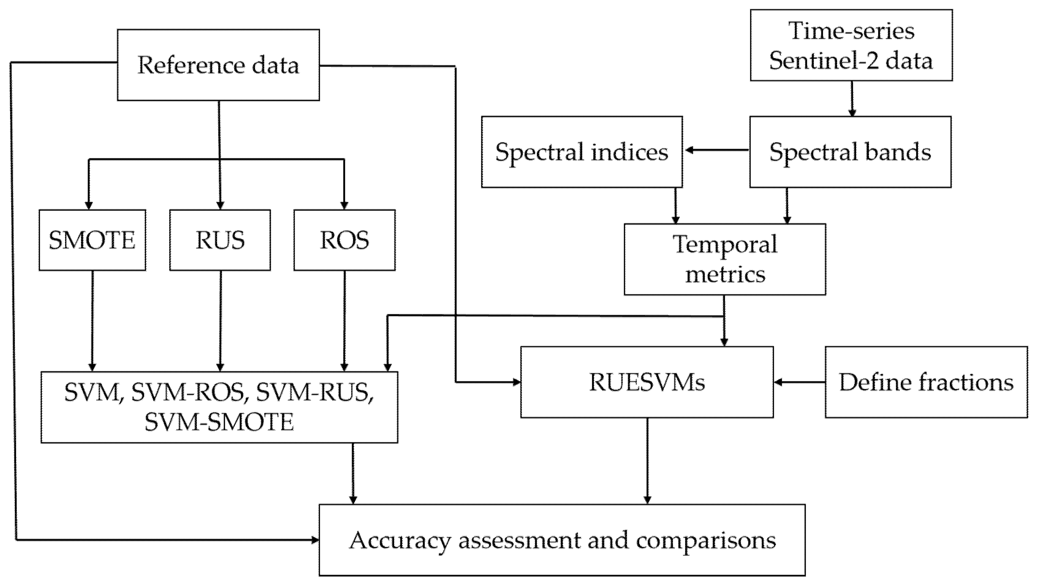
The methodology of the present research contains seven stages (Figure 2) as follows: (1) Acquiring Sentinel-2 images for the study sites and implementing the preprocessing steps; (2) Calculating spectral indices and temporal metrics; (3) Analyzing the distribution of LC classes and defining fractions for different LC classes; (4) Implementing the RUESVMs method to generate LC maps; (5) Calculating the accuracy assessment metrics; (6) Analyzing the results to select the most useful fractions; (7) Comparing the performance of RUESVMs with the other state-of-the-art methods (e.g., SVM-ROS, SVM-RUS, and SVM-SMOTE).

3.1. Input Features for LC Classification

Five commonly used spectral indices, including the NDVI [46], GNDVI [47], SAVI [48], NDBI [49,50], and NDWI [51], along with the main spectral bands of Sentinel-2 (see Section 2.2) were used for LC classification (the corresponding formulas of these indices are provided in Table 2). It has been demonstrated that the temporal metrics (e.g., the median value) are helpful in filling the gaps due to missing data and improving the LC classification by considering the phenological differences of LC types [40,52]. Therefore, the 20th, 50th (i.e., median) and 80th percentiles of ten spectral bands of Sentinel-2 and the five spectral indices were used in the classification. Instead of minimum and maximum values, the 20th and 80th percentiles were employed to decrease the effects of atmospheric contamination, residual clouds, and shadows. In total, 45 temporal metrics (i.e., per-pixel 20th, 50th, and 80th percentiles composites of each of the spectral bands and spectral indices) for each 10 m Sentinel-2 pixel location were utilized.

3.2. RUESVMs

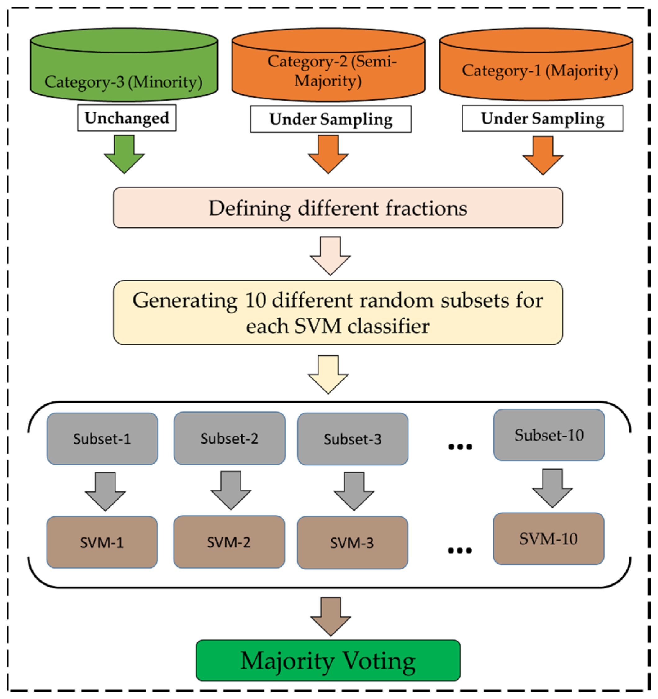
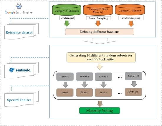
Flowchart of the proposed method (RUESVMs) to address the class imbalance problem in LC mapping is illustrated in Figure 3. The RUESVMs method is an ensemble-based algorithm, developed by integrating random under-sampling of majority classes and an ensemble of SVMs. Fully balancing the original imbalanced data using conventional under-sampling methods may result in removal of some useful information [28], which can change the decision boundary in an inappropriate way to make distinction between some classes, which in turn reduces the accuracy. Therefore, the RUESVMs method, by incorporating the best possible balance between the minority and majority classes, tries to achieve a high level of accuracy for both categories without losing useful information at the same time. In order to choose the best balance, it is possible to define some fractions according to which the majority and minority samples are selected (discussed in Section 3.4).
The RUESVMs method creates an ensemble of SVM classifiers that each is trained by a randomly under sampled subset of the original imbalanced data based on the defined fractions, and finally combines the output of the SVM classifiers using majority voting. The main steps in implementing the RUESVMs are as follows:
(1)
The fractions of LC classes are defined.
(2)
Based on the fractions, samples of original imbalanced data are randomly and repeatedly (with replacement) extracted. In this study, 10 different random subsets of the original data are generated for each fraction.
(3)
An SVM classifier is built for each of these 10 subsets. The radial basis function is used as kernel function, and the values of its parameters (i.e., cost and gamma) are selected after some preliminary analyses.
(4)
Using the built SVM classifiers, 10 LC maps are generated from the Sentinel-2 images.
(5)
The produced LC maps are combined using a majority voting strategy and the final LC map is generated.
The main objective of RUESVMs is to prevent possible information loss, as a common issue in traditional under-sampling methods, and provide a high level of accuracies for both the majority and minority classes by building a diverse ensemble of SVM classifiers from a series of independent random subsets of the original data. The code to apply RUESVMs for LC mapping in the GEE platform is provided in Supplementary Materials (Supplementary Materials S1).

3.3. The LC Class Fractions

Within the RUESVMs framework (Figure 3), it is possible to define any desired proportion of minority and majority classes to include in the random subsets. To be short and concise, 100 different fractions of LC classes were defined and the performance of RUESVMs with different fractions was evaluated to find the best possible proportion(s). An overview of the defined fractions is provided in Table 3 (see Supplementary Materials S2 and S3 for the complete list). Based on the LC classes distribution for Site-1 (Table 1), the LC classes were divided into three categories: Category-1 (majority classes), including the agriculture and grassland classes; Category-2 (semi-majority classes) including the barren and built-up classes; Category-3 (minority classes) including the road, urban vegetation, and water classes. Since the RUESVMs method is an under-sampling method, different possible combinations of Category-1 and Category-2 were only investigated in this study, and Category-3 (minority classes) left unchanged. For Site-2, similar to Site-1, different possible combinations of Category-1 (majority classes: agriculture and barren classes) and Category-2 (semi-majority classes: built-up and grassland classes) were only investigated, and Category-3 (minority classes: road, urban-vegetation, water, forest, and snow/ice classes) left unchanged.

3.4. Accuracy Assessment and Comparison

The confusion matrix was used to evaluate accuracy of the LC maps produced by RUESVMs. Accordingly, User Accuracy (UA), Producer Accuracy (PA), and Overall Accuracy (OA) were calculated over the validation datasets. The readers are referred to [53] for the explanation and formula of these metrics. The Geometric Means of UAs and PAs (GM-UA and GM-PA, respectively) were also calculated. The rationale of choosing these metrics was that they provide less bias toward majority classes when evaluating the classification accuracy of imbalanced data and, thus, are more suitable for the corresponding applications [26,54]. A small geometric mean value shows an inferior performance of the given classification method for at least one LC class [53].
In this study, the performance of RUESVMs was also compared with the traditional SVM and SVM combined with the three well-known data balancing techniques, including the Random Over-Sampling (ROS) [55], Random Under-Sampling (RUS) [56], and Synthetic Minority Over-sampling Technique (SMOTE) [57]. In the ROS method, as a straightforward oversampling approach, the classes are balanced by randomly replicating rare instances from the minority classes [55]. RUS, as a non-heuristic method, addresses the class imbalance problem by eliminating instances from the majority classes [56]. SMOTE generates new synthetic instances for the minority classes through convex mixtures of neighboring instances [57]. Along the connecting lines between a given sample and its k nearest neighbors in the feature space, it randomly creates artificial instances for that class. These three methods were implemented in R software [58] using the UBL package [59]. Several initial experiments were implemented to find the most optimum k value for SMOTE when the proposed method was compared with SVM-SMOTE. For Site-1 and Site-2, the best k values were selected as 5 and 7, respectively.

3.5. RUESVSMs Implementation

The procedure of RUESVMs implementation in the GEE platform for LC mapping with Sentinel-2 images in two experiment sites, comprises the following eight main steps: (1) insert the Sentinel-2 images and training data to GEE; (2) define fractions of LC classes; (3) perform random under-sampling of the original training data according to the defined fractions in step 2; (4) build an SVM classifier for the sampled data in step 3; (5) classify the Sentinel-2 data by the built SVM; (6) independently repeat steps 3–5 10 times; (7) conduct decision fusion of the classified labels based on majority voting to derive the final LC map; (8) perform accuracy assessment and comparison of the results with those of the traditional SVM, and the three integrated forms of SVM, including SVM-ROS, SVM-RUS, and SVM-SMOTE. Since an individual random division of the sampled pixels into training and validation subsets and implementation of a typical classifier (e.g., RUESVMs) cause a biased performance, the experiments were repeated 50 times with randomly divided original reference samples into training (50%) and validation (50%) datasets. Accordingly, the averaged accuracy metrics of different methods over 50 iterations are finally reported.

4. Results

4.1. Site-1

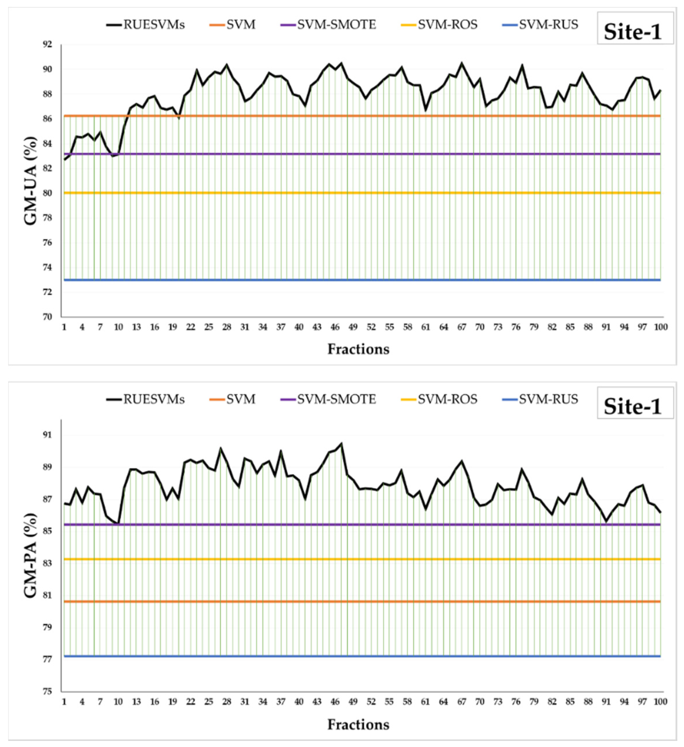
The RUESVMs method was applied to Site-1 with 100 different fractions, and the corresponding accuracies were assessed, where the complete results are demonstrated in Supplementary Materials S4. Comparing the results of 100 different fractions, it was observed that the fraction number 47 (RUESVMs-47) provided the best performance using 50% of Category-1, 70% of Category-2, and 100% of Category-3. The second best case was for the fraction number 27 (RUESVMs-27), which included 30%, 70%, and 100% of Category-1, Category-2, and Category-3, respectively. The three OA, GM-PA, and GM-UA values obtained from the RUESVMs-47 and RUESVMs-27 were above 89%, indicating high potential of the proposed algorithm for delineating both the minority and majority classes. According to Table 4, the results clearly demonstrate that RUESVMs-47 and RUESVMs-27 considerably improved the accuracy of the minority classes without reducing the accuracy of the majority classes, which is the main aim of the learning from imbalanced data [54]. Among 100 different fractions (Supplementary Materials S4), fraction number 1 (RUESVMs-1) provided the worst performance using 10% of Category-1, 10% of Category-2, and 100% of Category-3.
Four different versions of the SVM algorithm, including SVM, SVM-ROS, SVM-RUS, and SVM-SMOTE, were also implemented and applied to Site-1. As is clear from Table 4, although SVM-SMOTE provided the best results among these benchmark methods, both the RUESVMs-47 and RUESVMs-27 outperformed SVM-SMOTE. RUESVMs-47, respectively, increased the OA, GM-PA, and GM-UA values by approximately 4.2 percentage points, 5 percentage points, and 7.3 percentage points compared to SVM-SMOTE. More specifically, the UA values obtained from RUESVMs-47 for the classes of road, urban-vegetation, and water were 91.4%, 81.2%, and 99.2%, respectively, while the UA values of SVM-SMOTE for these classes were 71.8%, 66.8%, and 100%, respectively. Additionally, the PA values obtained from RUESVMs-47 for the minority classes were 85.8% (road), 87.4% (urban-vegetation), and 100% (water), which are considerably higher than those obtained from SVM-SMOTE.
The comparison between RUESVMs-47 and SVM-SMOTE for the majority classes was interesting. Although RUESVMs-47 yielded 2.1 percentage points and 1.5 percentage points lower UA values for the agriculture and grassland classes compared to those obtained from SVM-SMOTE, it yielded 16.2 percentage points and 0.5 percentage points higher UA values for the barren and built-up classes (semi-majority classes). According to the PA values, the results also showed that the RUESVMs-47 method increased the PA values of the agriculture, barren, built-up, and grassland classes by 6.5 percentage points, 4.1 percentage points, 4 percentage points, and 15.7 percentage points, respectively, compared to SVM-SMOTE.

4.2. Site-2

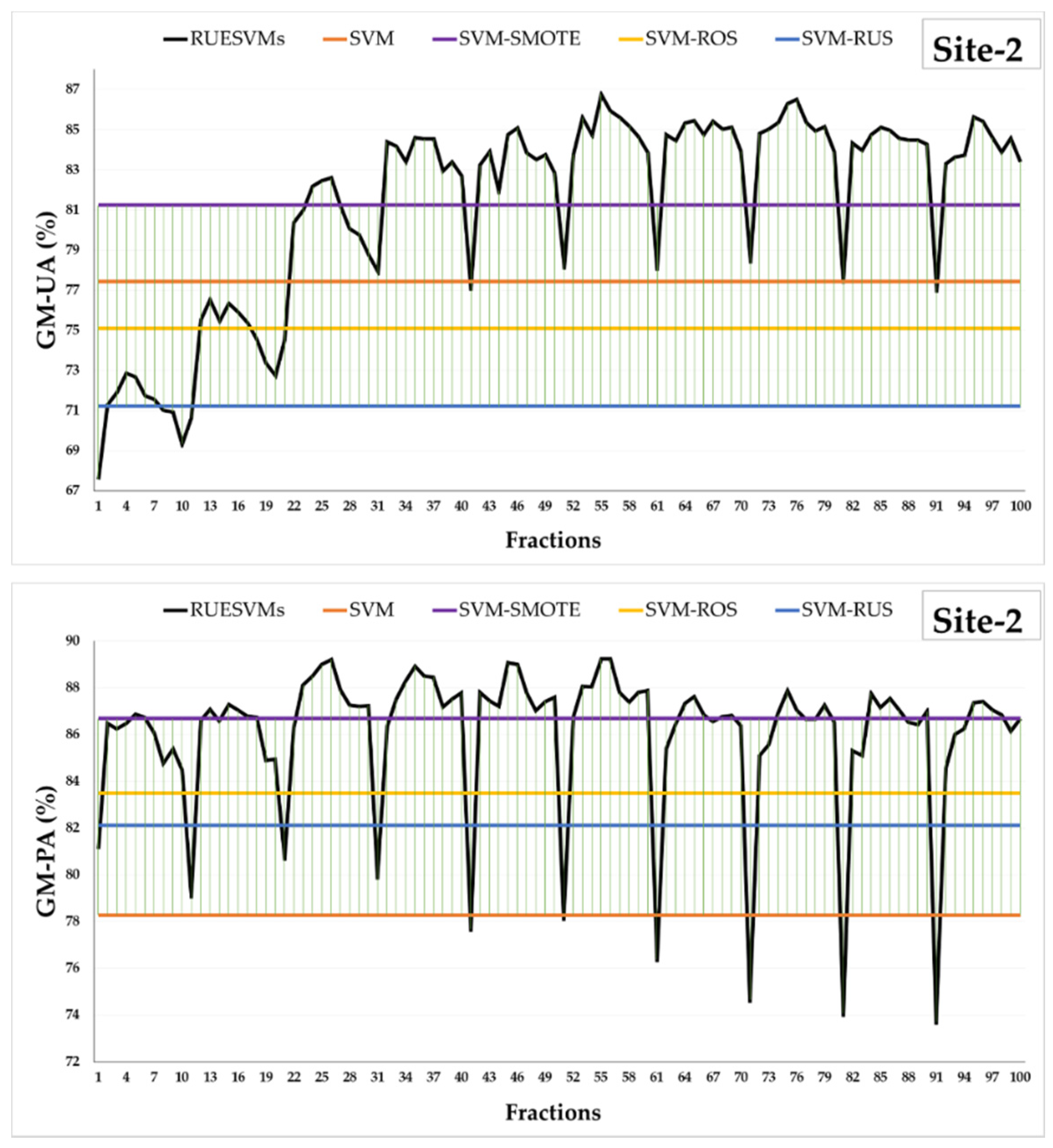
Similar to Site-1, the proposed method was applied to Site-2 with 100 different fractions and the relevant accuracies were evaluated against the four different benchmark methods (see Supplementary Materials S5). It was observed that the fraction number 55 (RUESVMs-55) provided the best performance using 60% of Category-1, 50% of Category-2, and 100% of Category-3, followed by RUESVMs-56, which included 60%, 60%, and 100% of Category-1, Category-2, and Category-3, respectively. Both fractions resulted in high accuracies for the rare classes without reducing the accuracy of majority classes (see Table 5); all the three OA, GM-PA, and GM-UA values for both fractions were above 85%. Among 100 different fractions (Supplementary Materials S5), fraction number 11 (RUESVMs-11) provided the worst performance using 20% of Category-1, 10% of Category-2, and 100% of Category-3.
As illustrated in Table 5, both RUESVMs-55 and RUESVMs-56 outperformed SVM-SMOTE, as the best performed benchmark method, where RUESVMs-55 improved OA, GM-PA, and GM-UA values by approximately 5.7 percentage points, 2.5 percentage points, and 5.6 percentage points, respectively. In the case of the minority classes, the UA values of RUESVMs-55 for the classes of road, urban-vegetation, water, forest, and snow/ice were 67.9%, 70.4%, 76.6%, 96.3% and 100%, respectively, while the UA values of SVM-SMOTE for these classes were 45.5%, 58.7%, 94.7%, 91%, and 100%, respectively. Furthermore, the PA values of RUESVMs-55 for these minority classes were 93.7%, 78.5%, 86%, 88.7%, and 100%, respectively. These were comparable with those obtained from SVM-SMOTE.
Regarding the majority classes, although RUESVMs-55 resulted in approximately 0.5 percentage points, 14.6 percentage points, and 7.4 percentage points higher UA values for the barren, built-up, and grassland classes, it provided 8.6 percentage points lower UA value for the agriculture class compared to SVM-SMOTE. Moreover, it was observed that RUESVMs-55 increased the PA values of the agriculture, barren, and built-up classes by 5.6 percentage points, 20.7 percentage points, and 11.9 percentage points compared to SVM-SMOTE, and decreased the PA value of the grassland class by 7.3 percentage points.

5. Discussion

The need for accurate LC classification using remote sensing technology, coupled with the potential of improving the accuracy using time-series of Sentinel-2 data, increase the need for effective computational resources and processing methods. The GEE platform, as a cloud-based computing environment [16,42], efficiently resolves several issues in LC classification using remote sensing data. Thus, the GEE platform was applied in this study to implement RUESVMs. This enables widespread availability of the RUESVMs approach and gives users the ability to process long time-series data over relatively large areas for LC mapping. By using GEE, as a big data processing platform, obtaining and processing data for each of the experimental sites took only few minutes. Conducting the same implementations using traditional image acquisition and processing methods would definitely be a time- and effort-consuming task.
The experiments demonstrated the efficiency of RUESVMs in dealing with class imbalance problem and improving LC classification accuracy, specifically for the minority classes. Comparing the results of the most accurate RUESVMs (RUESVMs-47 in Site-1 and RUESVMs-55 in Site-2) and the most accurate benchmark method (SVM-SMOTE), it was observed that the accuracy assessment metrics (i.e., OA, GM-PA, and GM-UA) were relatively higher for the proposed method. On average, in Site-1, RUESVM-47 provided an approximate 5.3 percentage point increase in these metrics in comparison to SVM-SMOTE, and in Site-2, RUESVMs-55 provided about a 4.6 percentage point increase in these metrics compared to SVM-SMOTE. Moreover, visual assessment and comparison of generated maps also showed higher performances of the proposed method than the most accurate benchmark method (Supplementary Materials S6).
Figure 4 and Figure 5 show the GM-UA and GM-PA values of the RUESVMs method over different fractions compared to the benchmark methods across the two study sites. As is clear from those figures, there are repeated patterns of both GM-UA and GM-PA values over almost every ten times of fractions. Those fractions divide the defined fractions (100) into 10 bunches of fractions, each including 10 individual fractions, and reach to pick points in the middle of every branch. This indicates that a moderate fraction from the three categories in both datasets results in better accuracy than a biased exercise of fractions with a very small (or large) number of samples from some categories.
In Site-1, the most accurate LC mapping result was obtained using 50% and 70% of the samples belonging to the majority classes and all samples of the minority classes. On the other hand, in Site-2, the best classifier performance was obtained by randomly sampling 60% and 50% of the samples belonged to the majority classes and 100% of the minority classes. Our experiments showed that the performance of RUESVMs varies over different fractions and it could not provide a high level of accuracy for both majority and minority classes in all fractions. For instance, based on Figure 5, the GM-UA and GM-PA values reach higher values when the fractions of Category-1 and Category-2 are moderate (e.g., RUESVMs-45 and RUESVMs-55); however, when using 10% for Category-2 (e.g., RUESVMs-91 and RUESVMs-81), the values of GM-UA and GM-PA decrease sharply. This indicates that a moderate fraction from these categories resulted in far better accuracy than a biased exercise of fractions with a very large number of samples from Category-1 and a small number of samples from Category-2. Due to the ensemble structure of RUESVMs, coupled with random sampling by replacement, it is possible to extract almost all the information of samples belonging to the majority classes, which will eventually lead to the appropriate accuracy. The lowest accuracies in Site-1 and Site-2 were obtained for scenarios 1 and 11, respectively. Scenarios 1 and 11 were very similar in terms of the number of samples taken from the majority and semi-majority classes (Categories 1–2), and both had the almost same number of samples of the majority and minority classes through the random under-sampling. In fact, using a small fraction of the majority and semi-majority classes led to the construction of a weak classifier due to the lack of sufficient data. On the other hand, the accuracy of the minority classes was reduced when a large portion of the samples was used from the majority classes. In summary, since the sampled reference data for image classification tasks are very different in terms of the imbalance ratio, number of LC classes, and number of samples per LC class, providing a robust approach for selecting the optimal fractions for broad settings is a very challenging task. Therefore, it is necessary to investigate different fractions to achieve the optimal fraction for a given setting.
Among different LC classes at two study sites, the best result was achieved for the urban-vegetation class, for which the proposed method provided approximately 14.4 percentage points and 11.7 percentage points higher UA values compared to SVM-SMOTE, for Site-1 and Site-2, respectively (see Table 4 and Table 5). In terms of the PA values, RUESVMs provided 5.1 and 6.1 higher values for the urban-vegetation class over Site-1 and Site-2, respectively. The reason might be related to the reduction in the instances of the agriculture and grassland classes, because they have similar spectral responses with that of the urban-vegetation class. Therefore, high imbalance ratios among these classes could lead to low accuracy of the class with lower instances. The lower accuracy of SVM-SMOTE was potentially related to the fact that the synthetic instances in the SMOTE method [57] might be generated close to majority instances in the feature space and, thus, misclassification can occur for the minority classes.
All the classifiers provided good results for the water class in terms of both UA and PA, which was reasonable because of the distinguishable spectral response of this class from other LC classes as well as the high ability of the NDWI index in extracting the water class [51]. In Site-2, however, SVM-SMOTE provided the best results for the water class, which could be linked to the possibility of creating new and accurate instances in the neighborhood of this class by the SMOTE algorithm. However, this is not possible for other minority classes, such as roads and urban-vegetation due to their complexity. In fact, although SVM-SMOTE provided better results for the water class in Site-2, it exhibited lower accuracies for the road and urban-vegetation classes compared to RUESVMs-55. The RUESVMs-55 method provided acceptable and balanced results for all the minority classes. It also provided better accuracy for the majority classes, which can be explained by its ensemble background and structure.
Based on previous studies, increasing the accuracy of minority classes usually leads to a reduction in the OA values. For example, previous studies reported an increase in PA without improvement in UA or OA metrics [18,60]. In contrast, the results obtained in this study demonstrated that the values for all overall accuracy metrics (i.e., OA, GM-PA, and GM-UA) as well as both UA and PA accuracies could be further increased by applying RUESVMs. Although a few studies could effectively handle the class imbalance [61,62], their performances were lower than the proposed method. Additionally, since multiple studies [63,64] did not apply the geometric mean metric in the validation step, the findings of the present work cannot be statistically compared with those of the other works.
Regarding suggestions for further research, we propose studying the performance of the RUESVMs method in different areas with different LC class distribution, especially for large-scale LC mapping. Future studies should also evaluate the accuracy of the proposed method when other ML algorithms, such as decision trees and random forest, are being utilized. Additionally, we recommend investigating the combination of the RUESVMs and an oversampling algorithm (e.g., SMOTE) for potential improvement in LC mapping.

6. Conclusions

In this study, the RUESVMs algorithm was proposed and investigated for LC mapping using time-series of Sentinel-2 images within the GEE platform. The performance of RUESVMs was compared against four benchmark methods, including traditional SVM, SVM-ROS, SVM-RUS, and SVM-SMOTE methods. The results revealed that the RUESVMs method considerably outperforms the benchmarks methods. Specifically, in comparison to the most accurate benchmark method (i.e., SVM-SMOTE), RUESVMs provided approximately 4.95 percentage points, 3.75 percentage points, and 6.45 percentage points higher values for OA, GM-PA, and GM-UA, respectively. In summary, three major conclusions can be drawn from this study. First, with regard to the great ability of the GEE cloud computing platform in dealing with big time-series data, LC mapping can be accomplished easily in this platform. Second, applying the RUESVMs method can improve LC classification accuracy. RUESVMs not only increased the accuracy of minority classes, it also increased the accuracy of majority classes. Third, incorporating the best possible balance between the minority and majority classes leads to the achievement of the highest possible accuracy for both minority and majority classes at the same time.

Supplementary Materials

The following are available online at https://www.mdpi.com/2072-4292/12/21/3484/s1, Supplementary Materials include: (1) Scripts for implementing RUESVMs for LC mapping using time-series Sentinel-2 images in the GEE platform; (2) Complete list of the defined LC class fractions for Site-1; (3) Complete list of the defined LC class fractions for Site-2; (4) Accuracy assessment results of different RUESVMs scenarios and the benchmark methods in Site-1; (5) Accuracy assessment results of different RUESVMs scenarios and the benchmark methods in Site-2; (6) LC maps of the most accurate RUESVMs fraction (i.e., RUESVMs-47) and the most accurate benchmark method (i.e., SVM-SMOTE) for Site-1; (7) LC maps of the most accurate RUESVMs fraction (i.e., RUESVMs-55) and the most accurate benchmark method (i.e., SVM-SMOTE) for Site-2; (8) Topographical characteristics (i.e., Slope angle and aspect) of the Site-1; (9) Topographical characteristics (i.e., Slope angle and aspect) of the Site-2.

Author Contributions

Conceptualization, H.E., A.N., M.A. (Mohsen Azadbakht); methodology, H.E., A.N.; software, H.E.; validation, A.N.; data curation, H.E.; formal analysis, J.B., M.A. (Meisam Amani); writing—original draft preparation, H.E., A.N.; writing—review and editing, M.A. (Mohsen Azadbakht), J.B., M.A. (Meisam Amani); supervision, J.B., M.A. (Mohsen Azadbakht); funding acquisition, A.N., J.B. All authors have read and agreed to the published version of the manuscript.

Funding

This research was jointly funded by the National Key Research and Development Program of China under grant (2016YFC0500201-06), the National Natural Science Foundation project of China (41701432, 41631180), the Strategic Priority Research Program of the Chinese Academy of Sciences (CAS) (XDA19030303), the CAS “Light of West China” Program, the Youth program of Institute of Mountain Hazards and Environment, CAS (SDS-QN-1902), the Youth Innovation Promotion Association CAS (Grant 2019365), and the CAS-TWAS president’s fellowship for international doctoral students.

Conflicts of Interest

The authors declare no conflict of interest.

References

  1. Mercier, A.; Betbeder, J.; Rumiano, F.; Baudry, J.; Gond, V.; Blanc, L.; Bourgoin, C.; Cornu, G.; Marchamalo, M.; Poccard-Chapuis, R. Evaluation of sentinel-1 and 2 time series for land cover classification of forest–agriculture mosaics in temperate and tropical landscapes. Remote Sens. 2019, 11, 979. [Google Scholar] [CrossRef] [Green Version]
  2. Naboureh, A.; Moghaddam, M.H.R.; Feizizadeh, B.; Blaschke, T. An integrated object-based image analysis and ca-markov model approach for modeling land use/land cover trends in the sarab plain. Arab. J. Geosci. 2017, 10, 259. [Google Scholar] [CrossRef]
  3. Ghorbanzadeh, O.; Valizadeh Kamran, K.; Blaschke, T.; Aryal, J.; Naboureh, A.; Einali, J.; Bian, J. Spatial prediction of wildfire susceptibility using field survey gps data and machine learning approaches. Fire 2019, 2, 43. [Google Scholar] [CrossRef] [Green Version]
  4. Moharrami, M.; Naboureh, A.; Gudiyangada Nachappa, T.; Ghorbanzadeh, O.; Guan, X.; Blaschke, T. National-scale landslide susceptibility mapping in austria using fuzzy best-worst multi-criteria decision-making. ISPRS Int. J. Geoinf. 2020, 9, 393. [Google Scholar] [CrossRef]
  5. Congalton, R.G.; Gu, J.; Yadav, K.; Thenkabail, P.; Ozdogan, M. Global land cover mapping: A review and uncertainty analysis. Remote Sens. 2014, 6, 12070–12093. [Google Scholar] [CrossRef] [Green Version]
  6. Thanh, H.N.T.; Doan, T.M.; Tomppo, E.; McRoberts, R.E. Land use/land cover mapping using multitemporal sentinel-2 imagery and four classification methods—A case study from dak nong, vietnam. Remote Sens. 2020, 12, 1367. [Google Scholar] [CrossRef]
  7. Ienco, D.; Gaetano, R.; Interdonato, R.; Ose, K.; Minh, D.H.T. Combining sentinel-1 and sentinel-2 time series via rnn for object-based land cover classification. In Proceedings of the IGARSS 2019—2019 IEEE International Geoscience and Remote Sensing Symposium, Yokohama, Japan, 28 July–2 August 2019. [Google Scholar]
  8. Griffiths, P.; Nendel, C.; Hostert, P. Intra-annual reflectance composites from sentinel-2 and landsat for national-scale crop and land cover mapping. Remote Sens. Environ. 2019, 220, 135–151. [Google Scholar] [CrossRef]
  9. Xiong, J.; Thenkabail, P.; Tilton, J.; Gumma, M.; Teluguntla, P.; Oliphant, A.; Congalton, R.; Yadav, K.; Gorelick, N. Nominal 30-m cropland extent map of continental africa by integrating pixel-based and object-based algorithms using sentinel-2 and landsat-8 data on google earth engine. Remote Sens. 2017, 9, 1065. [Google Scholar] [CrossRef] [Green Version]
  10. Devaux, N.; Crestey, T.; Leroux, C.; Tisseyre, B. Potential of sentinel-2 satellite images to monitor vine fields grown at a territorial scale. OENO One 2019, 53, 51–58. [Google Scholar] [CrossRef]
  11. Rujoiu-Mare, M.R.; Olariu, B.; Mihai, B.A.; Nistor, C.; Săvulescu, I. Land cover classification in romanian carpathians and subcarpathians using multi-date sentinel-2 remote sensing imagery. Eur. J. Remote Sens. 2017, 50, 496–508. [Google Scholar] [CrossRef] [Green Version]
  12. Skakun, S.; Vermote, E.; Roger, J.-C.; Justice, C. Multispectral misregistration of sentinel-2a images: Analysis and implications for potential applications. IEEE Geosci. Remote Sens. Lett. 2017, 14, 2408–2412. [Google Scholar] [CrossRef] [PubMed]
  13. Storie, C.D.; Henry, C.J. Deep learning neural networks for land use land cover mapping. In Proceedings of the IGARSS 2018—2018 IEEE International Geoscience and Remote Sensing Symposium, Valencia, Spain, 22–27 July 2018; pp. 3445–3448. [Google Scholar]
  14. Qian, Y.; Zhou, W.; Yan, J.; Li, W.; Han, L. Comparing machine learning classifiers for object-based land cover classification using very high resolution imagery. Remote Sens. 2015, 7, 153–168. [Google Scholar] [CrossRef]
  15. Rogan, J.; Franklin, J.; Stow, D.; Miller, J.; Woodcock, C.; Roberts, D. Mapping land-cover modifications over large areas: A comparison of machine learning algorithms. Remote Sens. Environ. 2008, 112, 2272–2283. [Google Scholar] [CrossRef]
  16. Amani, M.; Mahdavi, S.; Afshar, M.; Brisco, B.; Huang, W.; Mohammad Javad Mirzadeh, S.; White, L.; Banks, S.; Montgomery, J.; Hopkinson, C. Canadian wetland inventory using google earth engine: The first map and preliminary results. Remote Sens. 2019, 11, 842. [Google Scholar] [CrossRef] [Green Version]
  17. Waldner, F.; Chen, Y.; Lawes, R.; Hochman, Z. Needle in a haystack: Mapping rare and infrequent crops using satellite imagery and data balancing methods. Remote Sens. Environ. 2019, 233, 111375. [Google Scholar] [CrossRef]
  18. Bogner, C.; Seo, B.; Rohner, D.; Reineking, B. Classification of rare land cover types: Distinguishing annual and perennial crops in an agricultural catchment in south korea. PLoS ONE 2018, 13, e0190476. [Google Scholar] [CrossRef] [Green Version]
  19. Galar, M.; Fernandez, A.; Barrenechea, E.; Bustince, H.; Herrera, F. A review on ensembles for the class imbalance problem: Bagging-, boosting-, and hybrid-based approaches. IEEE Trans. Syst. Man Cybern. Part C Appl. Rev. 2011, 42, 463–484. [Google Scholar] [CrossRef]
  20. Prati, R.C.; Batista, G.E.; Silva, D.F. Class imbalance revisited: A new experimental setup to assess the performance of treatment methods. Knowl. Inf. Syst. 2015, 45, 247–270. [Google Scholar] [CrossRef]
  21. Ortigosa-Hernández, J.; Inza, I.; Lozano, J.A. Measuring the class-imbalance extent of multi-class problems. Pattern Recognit. Lett. 2017, 98, 32–38. [Google Scholar] [CrossRef]
  22. Johnson, J.M.; Khoshgoftaar, T.M. Survey on deep learning with class imbalance. J. Big Data 2019, 6, 27. [Google Scholar] [CrossRef]
  23. Yijing, L.; Haixiang, G.; Xiao, L.; Yanan, L.; Jinling, L. Adapted ensemble classification algorithm based on multiple classifier system and feature selection for classifying multi-class imbalanced data. Knowl. Based Syst. 2016, 94, 88–104. [Google Scholar] [CrossRef]
  24. Azadbakht, M.; Fraser, C.; Khoshelham, K. Improved urban scene classification using full-waveform lidar. Photogramm. Eng. Remote Sens. 2016, 82, 973–980. [Google Scholar] [CrossRef]
  25. Feng, W.; Dauphin, G.; Huang, W.; Quan, Y.; Bao, W.; Wu, M.; Li, Q. Dynamic synthetic minority over-sampling technique-based rotation forest for the classification of imbalanced hyperspectral data. IEEE J. Sel. Top. Appl. Earth Obs. Remote Sens. 2019, 12, 2159–2169. [Google Scholar] [CrossRef]
  26. Azadbakht, M.; Fraser, C.S.; Khoshelham, K. Synergy of sampling techniques and ensemble classifiers for classification of urban environments using full-swaveform lidar data. Int. J. Appl. Earth Obs. Geoinf. 2018, 73, 277–291. [Google Scholar] [CrossRef]
  27. Mellor, A.; Boukir, S.; Haywood, A.; Jones, S. Exploring issues of training data imbalance and mislabelling on random forest performance for large area land cover classification using the ensemble margin. ISPRS J. Photogramm. Remote Sens. 2015, 105, 155–168. [Google Scholar] [CrossRef]
  28. Haixiang, G.; Yijing, L.; Shang, J.; Mingyun, G.; Yuanyue, H.; Bing, G. Learning from class-imbalanced data: Review of methods and applications. Expert Syst. Appl. 2017, 73, 220–239. [Google Scholar] [CrossRef]
  29. Sharififar, A.; Sarmadian, F.; Malone, B.P.; Minasny, B. Addressing the issue of digital mapping of soil classes with imbalanced class observations. Geoderma 2019, 350, 84–92. [Google Scholar] [CrossRef]
  30. Maldonado, S.; López, J.; Vairetti, C. An alternative smote oversampling strategy for high-dimensional datasets. Appl. Soft Comput. 2019, 76, 380–389. [Google Scholar] [CrossRef]
  31. Han, H.; Wang, W.Y.; Mao, B.H. Borderline-smote: A new over-sampling method in imbalanced data sets learning. In Advances in Intelligent Computing; Springer: Berlin/Heidelberg, Germany, 2005. [Google Scholar]
  32. Kuncheva, L.I.; Whitaker, C.J. Measures of diversity in classifier ensembles and their relationship with the ensemble accuracy. Mach. Learn. 2003, 51, 181–207. [Google Scholar] [CrossRef]
  33. Liu, X.-Y.; Wu, J.; Zhou, Z.-H. Exploratory undersampling for class-imbalance learning. IEEE Trans. Syst. ManCybern. Part B Cybern. 2008, 39, 539–550. [Google Scholar]
  34. Lin, Z.; Hao, Z.; Yang, X.; Liu, X. Several svm ensemble methods integrated with under-sampling for imbalanced data learning. In Proceedings of the International Conference on Advanced Data Mining and Applications, Dalian, China, 21–23 November 2009; Springer: Berlin/Heidelberg, Germany; pp. 536–544. [Google Scholar]
  35. Rakwatin, P.; Longépé, N.; Isoguchi, O.; Shimada, M.; Uryu, Y.; Takeuchi, W. Using multiscale texture information from alos palsar to map tropical forest. Int. J. Remote Sens. 2012, 33, 7727–7746. [Google Scholar] [CrossRef]
  36. Gómez, C.; White, J.C.; Wulder, M.A. Optical remotely sensed time series data for land cover classification: A review. Isprs J. Photogramm. Remote Sens. 2016, 116, 55–72. [Google Scholar] [CrossRef] [Green Version]
  37. Al-Fares, W. Historical Land Use/Land Cover Classification Using Remote Sensing: A Case Study of the Euphrates River Basin in Syria; University of Jena: Jena, Germany, 2013. [Google Scholar]
  38. Yang, X.; Zhao, S.; Qin, X.; Zhao, N.; Liang, L. Mapping of urban surface water bodies from sentinel-2 msi imagery at 10 m resolution via ndwi-based image sharpening. Remote Sens. 2017, 9, 596. [Google Scholar] [CrossRef] [Green Version]
  39. Thanh Noi, P.; Kappas, M. Comparison of random forest, k-nearest neighbor, and support vector machine classifiers for land cover classification using sentinel-2 imagery. Sensors 2018, 18, 18. [Google Scholar] [CrossRef] [Green Version]
  40. Amani, M.; Salehi, B.; Mahdavi, S.; Granger, J.E.; Brisco, B.; Hanson, A. Wetland classification using multi-source and multi-temporal optical remote sensing data in newfoundland and labrador, canada. Can. J. Remote Sens. 2017, 43, 360–373. [Google Scholar] [CrossRef]
  41. Mountrakis, G.; Im, J.; Ogole, C. Support vector machines in remote sensing: A review. ISPRS J. Photogramm. Remote Sens. 2011, 66, 247–259. [Google Scholar] [CrossRef]
  42. Gorelick, N.; Hancher, M.; Dixon, M.; Ilyushchenko, S.; Thau, D.; Moore, R. Google earth engine: Planetary-scale geospatial analysis for everyone. Remote Sens. Environ. 2017, 202, 18–27. [Google Scholar] [CrossRef]
  43. Huang, H.; Chen, Y.; Clinton, N.; Wang, J.; Wang, X.; Liu, C.; Gong, P.; Yang, J.; Bai, Y.; Zheng, Y. Mapping major land cover dynamics in beijing using all landsat images in google earth engine. Remote Sens. Environ. 2017, 202, 166–176. [Google Scholar] [CrossRef]
  44. Sidhu, N.; Pebesma, E.; Câmara, G. Using google earth engine to detect land cover change: Singapore as a use case. Eur. J. Remote Sens. 2018, 51, 486–500. [Google Scholar] [CrossRef]
  45. Ghorbanian, A.; Kakooei, M.; Amani, M.; Mahdavi, S.; Mohammadzadeh, A.; Hasanlou, M. Improved land cover map of iran using sentinel imagery within google earth engine and a novel automatic workflow for land cover classification using migrated training samples. ISPRS J. Photogramm. Remote Sens. 2020, 167, 276–288. [Google Scholar] [CrossRef]
  46. Rouse, J.; Haas, R.; Schell, J.; Deering, D. Monitoring vegetation systems in the great plains with erts. NASA Spec. Publ. 1974, 351, 309. [Google Scholar]
  47. Gitelson, A.A.; Kaufman, Y.J.; Merzlyak, M.N. Use of a green channel in remote sensing of global vegetation from eos-modis. Remote Sens Environ. 1996, 58, 289–298. [Google Scholar] [CrossRef]
  48. Huete, A. Huete, ar a soil-adjusted vegetation index (savi). Remote sensing of environment. Remote Sens. Environ. 1988, 25, 295–309. [Google Scholar] [CrossRef]
  49. Zha, Y.; Gao, J.; Ni, S. Use of normalized difference built-up index in automatically mapping urban areas from tm imagery. Int. J. Remote Sens. 2003, 24, 583–594. [Google Scholar] [CrossRef]
  50. Weigand, M.; Staab, J.; Wurm, M.; Taubenböck, H. Spatial and semantic effects of lucas samples on fully automated land use/land cover classification in high-resolution sentinel-2 data. Int. J. Appl. Earth Obs. Geoinf. 2020, 88, 102065. [Google Scholar] [CrossRef]
  51. McFeeters, S.K. The use of the normalized difference water index (ndwi) in the delineation of open water features. Int. J. Remote Sens. 1996, 17, 1425–1432. [Google Scholar] [CrossRef]
  52. Zhang, H.K.; Roy, D.P. Using the 500 m modis land cover product to derive a consistent continental scale 30 m landsat land cover classification. Remote Sens. Environ. 2017, 197, 15–34. [Google Scholar] [CrossRef]
  53. Congalton, R.G. A review of assessing the accuracy of classifications of remotely sensed data. Remote Sens. Environ. 1991, 37, 35–46. [Google Scholar] [CrossRef]
  54. He, H.; Garcia, E.A. Learning from imbalanced data. IEEE Trans. Knowl. Data Eng. 2009, 21, 1263–1284. [Google Scholar]
  55. Chawla, N.V. Data mining for imbalanced datasets: An overview. In Data Mining and Knowledge Discovery Handbook; Springer: Berlin/Heidelberg, Germany, 2009; pp. 875–886. [Google Scholar]
  56. Batista, G.E.; Prati, R.C.; Monard, M.C. A study of the behavior of several methods for balancing machine learning training data. ACM SIGKDD Explor. Newsl. 2004, 6, 20–29. [Google Scholar] [CrossRef]
  57. Chawla, N.V.; Bowyer, K.W.; Hall, L.O.; Kegelmeyer, W.P. Smote: Synthetic minority over-sampling technique. J. Artif. Intell. Res. 2002, 16, 321–357. [Google Scholar] [CrossRef]
  58. Team, R.C. R: A Language and Environment for Statistical Computting; R Foundation for Statistical Computing: Vienna, Austria, 2017; Available online: https://www.R-project.org (accessed on 21 April 2017).
  59. Branco, P.; Ribeiro, R.P.; Torgo, L. Ubl: An R package for utility-based learning. arXiv 2016, arXiv:1604.08079. [Google Scholar]
  60. Feng, W.; Huang, W.; Bao, W. Imbalanced hyperspectral image classification with an adaptive ensemble method based on smote and rotation forest with differentiated sampling rates. IEEE Geosci. Remote Sens. 2019, 16, 1879–1883. [Google Scholar] [CrossRef]
  61. Douzas, G.; Bacao, F.; Fonseca, J.; Khudinyan, M. Imbalanced learning in land cover classification: Improving minority classes’ prediction accuracy using the geometric smote algorithm. Remote Sens. 2019, 11, 3040. [Google Scholar] [CrossRef] [Green Version]
  62. Johnson, J.M.; Khoshgoftaar, T.M. Deep learning and data sampling with imbalanced big data. In Proceedings of the 2019 IEEE 20th International Conference on Information Reuse and Integration for Data Science (IRI), Los Angeles, CA, USA, 30 July–1 August 2019; pp. 175–183. [Google Scholar]
  63. Cenggoro, T.W.; Isa, S.M.; Kusuma, G.P.; Pardamean, B. Classification of imbalanced land-use/land-cover data using variational semi-supervised learning. In Proceedings of the 2017 International Conference on Innovative and Creative Information Technology (ICITech), Salatiga, Indonesia, 2–4 November 2017; pp. 1–6. [Google Scholar]
  64. Feng, W.; Boukir, S.; Huang, W. Margin-based random forest for imbalanced land cover classification. In Proceedings of the IGARSS 2019—2019 IEEE International Geoscience and Remote Sensing Symposium, Yokohama, Japan, 28 July–2 August 2019; pp. 3085–3088. [Google Scholar]
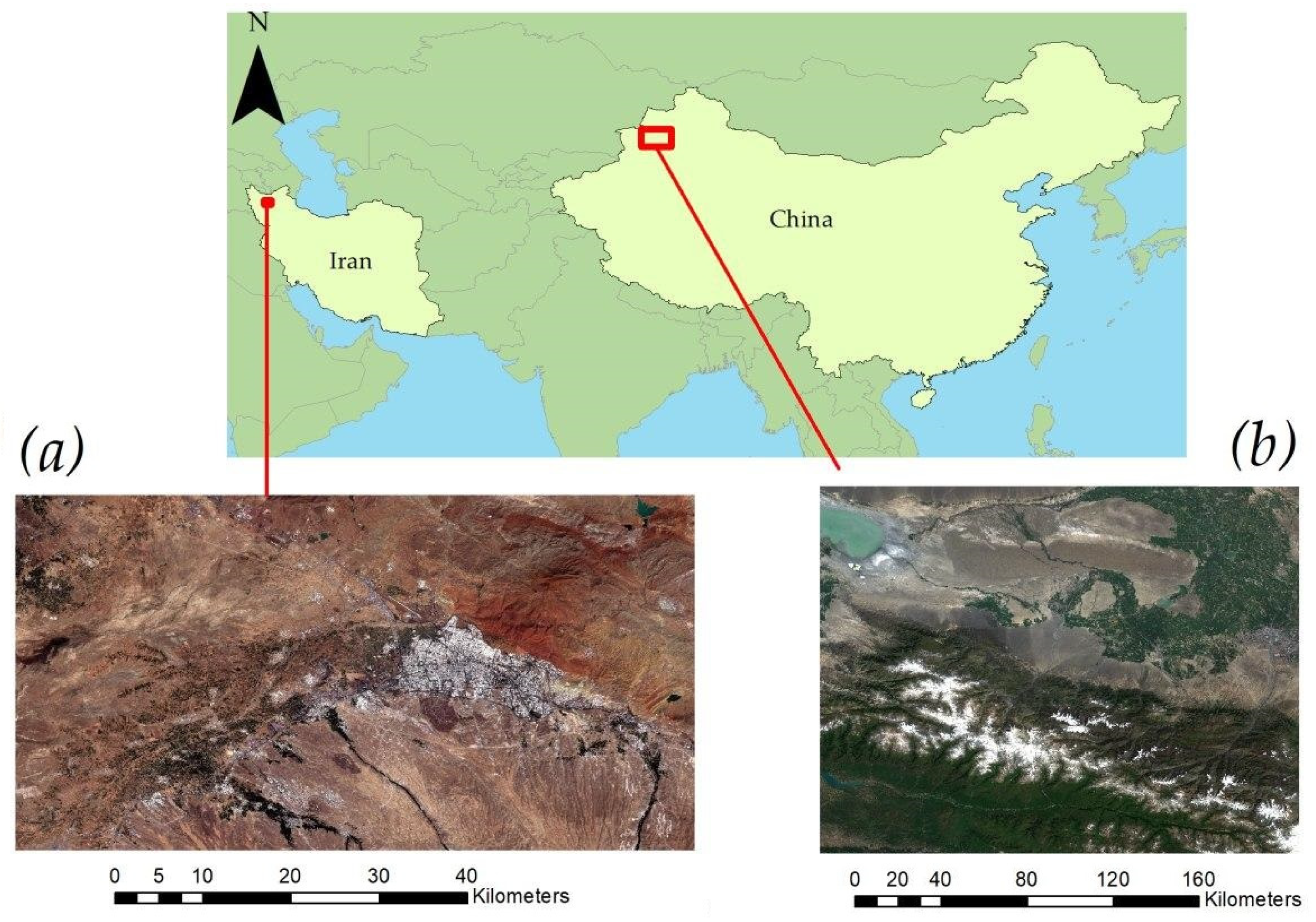
Figure 1. The RGB color composites (R: Band4, G: Band3, B: Band2) of the study areas: Site-1 (a) and Site-2 (b).
Remotesensing 12 03484 g001
Figure 2. The general workflow of the present research.
Remotesensing 12 03484 g002
Figure 3. The schematic representation of Random Under-sampling Ensemble of Support Vector Machines (RUESVMs).
Remotesensing 12 03484 g003
Figure 4. GM-UA and GM-PA values obtained from different RUESVMs scenarios and the benchmark methods (i.e., SVM, SVM-SMOTE, SVM-ROS, and SVM-RUS) over Site-1.
Remotesensing 12 03484 g004
Figure 5. GM-UA and GM-PA values obtained from different RUESVMs scenarios and the benchmark methods (i.e., SVM, SVM-SMOTE, SVM-ROS, and SVM-RUS) over Site-2.
Remotesensing 12 03484 g005
Table 1. Information of the reference sampled data for each study area.
LC ClassAgricultureBarrenBuilt-UpGrasslandRoadUrban-VegetationWaterForestSnow/Ice
Site-1291189184265764621--
Site-24033851691536251606560
Table 2. Formula of the spectral indices. Band numbers in the formulas refer to the Sentinel-2 bands. For Site-1 L is equal to 0.5 and for Site-2 L is equal to 0.428.
Spectral IndexFormula
NDVI(Band8 − Band4)/(Band8 + Band4)
GNDVI(Band8 − Band3)/(Band8 + Band3)
SAVI((Band8 − Band4)/(Band8 + Band4 + L)) × (1 + L)
NDBI(Band11 − Band8)/(Band11 + Band8)
NDWI(Band3 − Band8)/(Band3 + Band8)
Table 3. An overview of the defined LC class fractions for different categories.
ScenarioLC Class Fractions (%)
Category-1Category-2Category-3
11010100
21020100
31030100
41040100
51050100
61060100
71070100
81080100
91090100
1010100100
112010100
9910090100
100100100100
Table 4. Accuracy assessment (%) of the most accurate RUESVMs fractions and the benchmark methods over Site-1 (UA = user accuracy, PA = producer accuracy, OA = overall accuracy, GM = geometric means, RUESVMs = random under-sampling ensemble of support vector machines, SVMs = support vector machines, SMOTE = synthetic minority over-sampling technique, ROS = random over sampling, and RUS = random under-sampling).
MethodPer-Class MetricsLC ClassesOverall Metrics
AgricultureBarrenBuilt-upGrasslandRoadUrban-VegetationWaterOA (%)GM-UA (%)GM-PA (%)
RUESVMs-47UA (%)93.890.995.383.091.481.299.289.890.590.4
PA (%)95.882.690.192.685.887.4100
RUESVMs-27UA (%)96.888.897.179.689.27999.390.789.690.1
PA (%)95.480.885.892.788.389.4100
SVMUA (%)88.175.990.979.274.798.710084.986.380.6
PA (%)99.073.482.682.986.851.3100
SVM-SMOTEUA (%)95.974.794.884.571.866.810085.683.285.4
PA (%)89.378.586.176.986.982.3100
SVM-ROSUA (%)97.368.494.783.766.560.010082.38083.3
PA (%)82.680.082.571.286.982.3100
SVM-RUSUA (%)93.865.490.266.158.451.810074.87377.2
PA (%)76.263.277.167.087.075.7100
Table 5. Accuracy assessment (%) of the most accurate RUESVMs fractions and the benchmark methods over Site-2.
MethodPer-Class Metrics LC ClassesOverall Metrics
AgricultureBarrenBuilt-UpGrasslandRoadUrban-VegetationWaterForestSnow/IceOA (%)GM-UA (%)GM-PA (%)
RUESVMs-55UA (%)90.796.995.294.367.970.476.696.310091.286.889.2
PA (%)97.494.583.782.893.778.58688.7100
RUESVMs-56UA (%)89.595.893.192.865.6737794.59991.785.989.2
PA (%)96.793.181.281.293.979.788.691100
SVMUA (%)92.278.479.38763.145.089.083.994.684.777.478.3
PA (%)92.190.871.785.558.947.790.29292.3
SVM-SMOTEUA (%)99.396.480.686.945.558.794.79110085.581.286.7
PA (%)91.873.871.890.110072.494.895.695.9
SVM-ROSUA (%)97.387.285.884.84235.494.787.310082.775.183.5
PA (%)91.574.361.879.694.875.894.79096.1
SVM-RUSUA (%)96.985.386.885.339.22694.790.58879.671.282.1
PA (%)91.867.755.579.210075.094.787.4100
Publisher’s Note: MDPI stays neutral with regard to jurisdictional claims in published maps and institutional affiliations.