Article

Influence of Different Satellite Imagery on the Analysis of Riparian Leaf Density in a Mountain Stream

by
Giovanni Romano
,
Giovanni Francesco Ricci
* and
Francesco Gentile
Department of Agricultural and Environmental Sciences, University of Bari Aldo Moro, 70032 Bari, Italy
*
Author to whom correspondence should be addressed.
Remote Sens. 2020, 12(20), 3376; https://doi.org/10.3390/rs12203376
Submission received: 8 September 2020 / Revised: 7 October 2020 / Accepted: 13 October 2020 / Published: 15 October 2020
(This article belongs to the Section Environmental Remote Sensing)

Abstract

:
In recent decades, technological advancements in sensors have generated increasing interest in remote sensing data for the study of vegetation features. Image pixel resolution can affect data analysis and results. This study evaluated the potential of three satellite images of differing resolution (Landsat 8, 30 m; Sentinel-2, 10 m; and Pleiades 1A, 2 m) in assessing the Leaf Area Index (LAI) of riparian vegetation in two Mediterranean streams, and in both a winter wheat field and a deciduous forest used to compare the accuracy of the results. In this study, three different retrieval methods—the Caraux-Garson, the Lambert-Beer, and the Campbell and Norman equations—are used to estimate LAI from the Normalized Difference Vegetation Index (NDVI). To validate sensor data, LAI values were measured in the field using the LAI 2200 Plant Canopy Analyzer. The statistical indices showed a better performance for Pleiades 1A and Landsat 8 images, the former particularly in sites characterized by high canopy closure, such as deciduous forests, or in areas with stable riparian vegetation, the latter where stable reaches of riparian vegetation cover are almost absent or very homogenous, as in winter wheat fields. Sentinel-2 images provided more accurate results in terms of the range of LAI values. Considering the different types of satellite imagery, the Lambert-Beer equation generally performed best in estimating LAI from the NDVI, especially in areas that are geomorphologically stable or have a denser vegetation cover, such as deciduous forests.

Graphical Abstract

1. Introduction

Remote sensing is a technique for acquiring information on the Earth using different types of sensors located at variable distances [1]. Ever since the first remote sensing imagery became available, it has been used for environmental applications, such as land use, hydrology, geology, weather, climate, and vegetation studies [2,3]. Satellites and aircrafts equipped with optical, radar, or laser sensors (i.e., satellite platforms) are the most common means for collecting data on and studying Earth’s surface [4]. Along with these traditional remote sensing technologies, drones have recently been used to conduct environmental studies [5,6,7,8]. Satellite remote sensing, however, is still used to monitor large areas at regular intervals of time [9,10]. The main advantages of satellite imagery are that some platforms offer free access to data and the availability of different spatial and temporal resolutions [11]. The use of satellite imagery is, therefore, essential in contexts where the size of the area makes in-field monitoring expensive and time-consuming, as in the case of watersheds [12].
There are currently numerous satellite platforms operating; these carry different types of sensors with spatial and temporal resolutions that range from sub-metric to kilometric and from 30 min to weeks or months, respectively [13]. AVHRR, Sentinel, MODIS, Landsat, SPOT, Pleiades, and Ikonos are among the satellite platforms most commonly used to monitor vegetation features [13,14,15,16]. Given the wide variety of satellite imagery, it is important to choose the one most suited to the objectives of the study. A fundamental aspect to consider is the scale of the information that will be evaluated. In general, images with coarser resolutions may be used for regular vegetation patterns, whereas finer resolutions are required to study complex environments [17,18]. Mixed pixels may be a problem if the resolution is too coarse [19,20].
Vegetation indices (Vis), defined as algorithms to evaluate differences in plant canopy spectral characteristics [13], are used to quantitatively and qualitatively assess vegetation features using satellite remote sensing data. Different Vis may be used, depending on the satellite platform and pixel resolution. To evaluate their accuracy, Vis must be calibrated/validated with ground data [11]. The Leaf Area Index (LAI), defined as the one-sided leaf area per unit ground area, is one of the most commonly used indicators to evaluate leaf density on a horizontal surface area [21,22]. Since photosynthesis occurs in leaves, LAI is directly correlated with the conservation status of the plant system [23,24]. Moreover, LAI is indirectly correlated with certain processes that may disturb the state of the ecosystem, such as lack of nutrients in soil, geomorphological instability, and fires [25,26,27]. For all these reasons, the LAI is considered a critical parameter in ecosystem studies [13,28] and one which can be used to validate remote sensing data with in-field measurements. The LAI can be measured directly in the field through several methods, or it may be calculated from several Vis. Among the different Vis, the Normalized Difference Vegetation Index (NDVI) is the one most often used in forestry and agricultural studies, since it has a high correlation with the LAI [29,30,31,32]. One of the main problems in adopting the LAI-NDVI approach [33] is that there is no single equation to represent this relationship, because these indices have often been formulated for specific vegetation types [24].
Riparian ecosystems are complex environments characterized by narrow strips of vegetation with important ecological and ecosystem functions [34,35,36,37]. Among the ecosystem services provided by riparian areas, the maintenance of the geomorphological stability of the channels [38,39], and the protection of the watercourses against pollution and runoff coming from diffuse sources [40] are considered of interest inasmuch can support the achievement of the environmental objectives of the Water Framework Directive [41]. These aspects are more relevant, considering that (especially in the Mediterranean areas) human pressures, such as grazing, agricultural activities, and urbanization, lead to reduce riparian areas, negatively affecting the ecosystem services [42]. Satellite imagery can be used to map riparian ecosystems, as well as to monitor the effects of land management works, such as check dams and to detect critical sites, in which channel or riverbed erosion is taking place [27,43]. In such applications, a key point that needs to be deepened is the framework to be adopted, from the sampling design to the choice of the most appropriate satellite platform.
The aim of this study was to test the performance of three different resolution imagery, Landsat 8, Sentinel-2, and Pleiades 1A, in detecting the LAI in a Mediterranean area characterized by different land cover types. LAI measurements were carried out in the field using the LAI 2200 Plant Canopy Analyzer [44] using a suitable sampling design, while derived LAI values from Landsat 8, Sentinel-2, and Pleiades 1A imagery were retrieved using the Caraux-Garson, the Lambert-Beer, and the Campbell and Norman equations. The LAI-NDVI approach was adopted, fixing both the VI variable and the applied mathematical equations, given its recognized scientific robustness to better focus the analysis on the issue of the selection of the satellite imagery, which suits most the complex riparian environment.

2. Materials and Methods
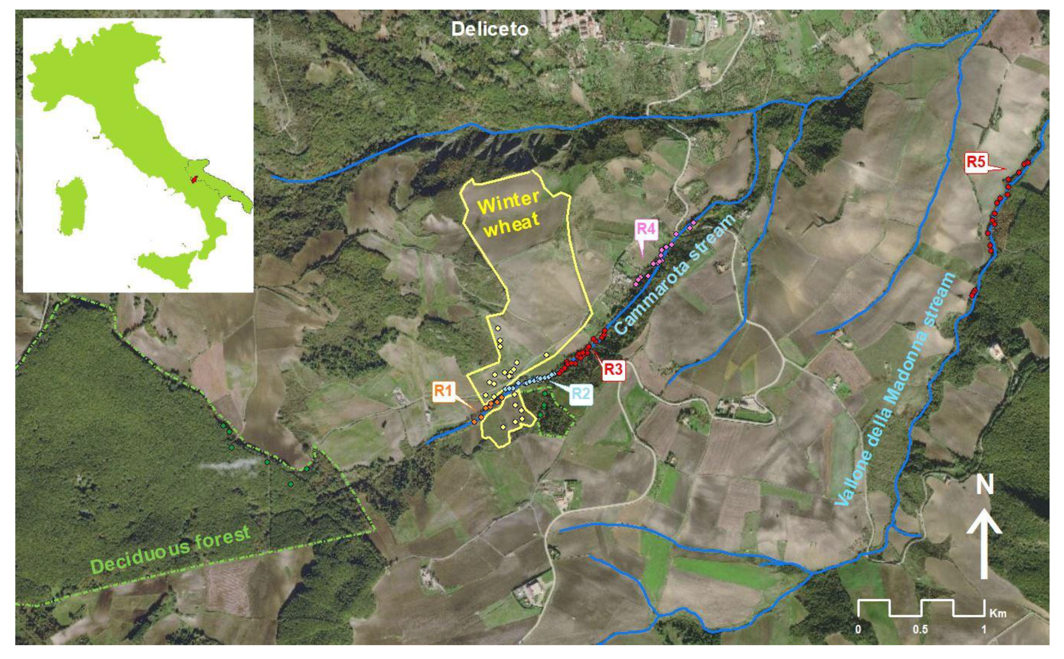
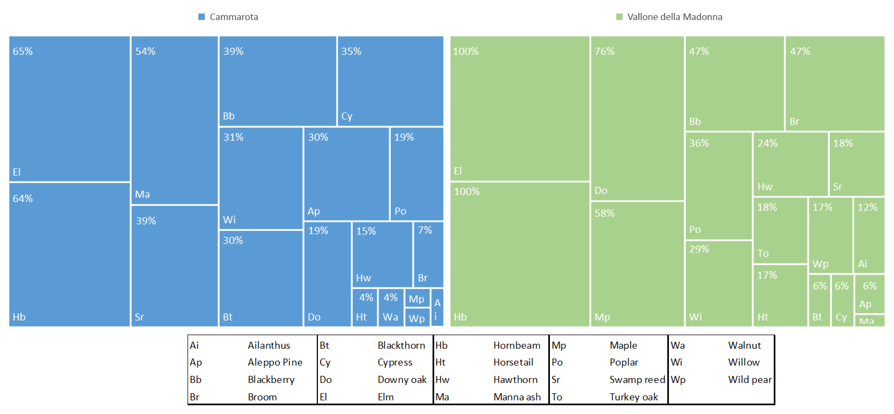
2.1. Study Area

Research was conducted in the upper part of the Carapelle watershed, close to the Deliceto municipality (northwestern Puglia) in Southern Italy (Figure 1). The Carapelle is a typical Mediterranean watershed that covers an area of about 982.6 km2, with a maximum altitude of 1075 m a.s.l. (average 540 m a.s.l.) and a mean watershed slope of 4.4%. In particular, the studied area has an altitude ranging from 934 and 284 m a.s.l. with a mean slope of 3.2%. Flysch formations constitute the mountainous areas, whereas clayey-sandy Plio-Pleistocene sediments characterize the alluvial plain [45]. The climate, typically Mediterranean, is characterized by mild, moist winters and warm, dry summers. The annual rainfall and average monthly temperatures range from 450 to 800 mm y−1 and from 10 to 16 °C, respectively [46]. Rainfalls, which are intense, of short duration and are concentrated in the autumn-spring months, determine the torrential hydrological regime of the main watercourses in the area [47].
The most frequent tree species in the riparian buffers are elm (Ulmus minor Mill.), hornbeam (Carpinus orientalis Mill.), and manna ash (Fraxinus ornus L.). Plant formations rich in poplar (Populus alba L.) and white willow (Salix alba L.) flank the watercourses, where the edaphic moisture conditions are favorable. Blackberry (Rubus ulmifolius Schott.) and common reed (Phragmites Australis Cav.) are the most frequently occurring shrubs (Figure 2).
Downy oak and hardwood (Quercus pubescens Wild and Quercus. Cerris L., respectively), along with pasture, meadow, and coniferous species, cover the higher slopes. Wheat cultivation, and to a lesser extent, agricultural crops and olive groves are the predominant cultivation systems in the plain and low hilly areas [48].
LAI values were measured in-situ at the Cammarota (CR) and Vallone della Madonna (R5) streams, both tributaries of the Carapelle Torrent, and in two surrounding areas, one covered by winter wheat (WW) fields and the other by a deciduous forest (DF). The watercourses, with narrow cross-sections and stratified vegetation, differ from one another in geomorphological stability, and consequently, in vegetation density. The CR is characterized by different vegetation patterns and degrees of erosion and by the presence of numerous check dams, which are severely damaged or destroyed. Along the monitored transect of the CR, there are 28 check dams, of which 15 are destroyed, 3 are damaged, and 10 are intact. The destroyed check dams are the main cause of active erosion processes along the stream [27]. Based on the severity of the erosion and on the conservation state of the check dams, the stream was divided into four reaches (R1–R4, Figure 1): Their features are described in Table 1. Along with R5, instead, check dams are intact, and vegetation is denser and well stratified, with no signs of riverbed erosion.

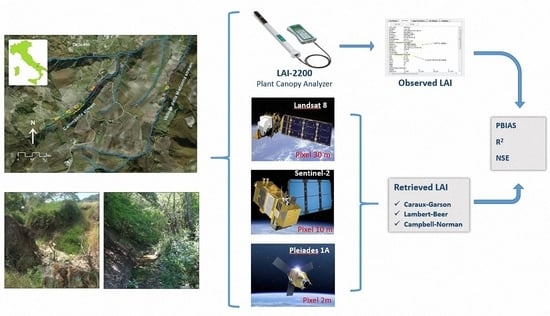
2.2. Field Data and Satellite Imagery

LAI values were measured in the field from May to July 2015, during the growing season and before crop harvest. A large LAI dataset was collected at each study site using the LAI 2200 Plant Canopy Analyzer [44], a sensor composed of five concentric rings. Readings were collected along several cross-sections of the monitored watercourses, for a width ranging from 10 m to 20 m, in one sensor mode for above and below readings, using a 90° view cap to avoid interference caused by the user’s shadow. One above-canopy reading was detected for every four below-canopy readings. Moreover, to take into account the slope of the study area the “measuring on slope” protocol was applied [44]. Other optical corrections were not applied, since the effect on the measurement is negligible for areas with a slope less than 30° [49]. The transects were conducted from one bank to the other at the site of a check dam and between two consecutive check dams. In the wheat fields and the forest area, readings were taken along a single direction, to obtain the most suitable overlap between field measurements and the satellite imagery acquired by the different sensors. A total of 82 field datasets were collected: 53 in CR, 11 in R5, 8 in DF, and 10 in WW. The acronym RV (Riparian Vegetation) is used henceforth to refer to CR and R5 together. A Garmin GPSMAP 76CSx was used to register the location of transects and check dam positions.
Multispectral data for this study is from medium- to high-resolution imagery provided by Landsat 8 (L8), Sentinel-2 (S-2), and Pleiades 1A (P1A) satellites. Considering the aims of this study, images with coarser resolutions were not used because larger pixel sizes could not detect riparian vegetation features adequately. The adopted L8 (30 m) and S-2 (10 m) medium resolution platforms are open access and guarantee excellent spatial and temporal coverage (Landsat from 1972, Sentinel from 2015). For these reasons, this satellite imagery is commonly used to carry out Vis studies and is of particular interest to both technicians and scientists [50]. In addition, P1A (2 m) high-resolution imagery was also used because it yields accurate Vis in forest environments [51,52,53].
The reduction of between scenes variability, due to different sensors acquisitions, was achieved by converting the imagery spectral digital number to top of atmosphere (TOA) reflectance. The advantages of using TOA reflectance arise from the necessity of better comparing remote sensing data acquired by different sensors at different times [48]. Also, TOA reflectance compensates different radiance values caused by different spectral bands, and lastly, corrects the variation in the Earth-Sun distance over the acquisition dates [54]. As suitable atmospheric aerosol data were not available for every image acquisition, all the sets of image data were not atmospherically corrected to top of canopy reflectance values.
Landsat data (https://landsat.usgs.gov/landsat-8) has been frequently used for land cover studies [55], but rarely for the analysis of riparian vegetation in streams with narrow cross-sections [27]. The cloud-free imagery used in this work, acquired by Landsat OLI sensors on 1 June and 3 July 2015, was downloaded using the Earth Explorer Get Data tool of the U.S. Geological Survey Landsat web page (http://earthexplorer.usgs.gov). L8 imagery data were corrected to TOA spectral radiance, using the radiance rescaling factors in the MTL file, and then converted to TOA reflectance, using the rescaling coefficients and the correction for the sun angle (https://www.usgs.gov/land-resources/nli/landsat/using-usgs-landsat-level-1-data-product).
The Sentinel satellite is an orbital wide-swath (290 km) imaging mission carrying an innovative Multispectral Imager (MSI), which provides a versatile set of 13 spectral bands from the visible to the shortwave infrared at 10 to 60 m spatial resolution. For the present work, a cloud-free Level 1C (Top-of-Atmosphere reflectance) image acquired on 28 July 2015 was downloaded from the ESA Sentinel-2 Pre-Operations Hub (https://scihub.copernicus.eu). The Level 1C of S2 imagery provided data already in TOA reflectance along with the parameters to eventually transform them into radiances (https://sentinel.esa.int/web/sentinel/user-guides/sentinel-2-msi/product-types/level-1c). The SNAP toolbox was used to process the visible, the near-infrared, and the shortwave infrared bands (10 m, 10 m, and 20 m spatial resolution, respectively) to produce a subset covering 3.7 km × 1.94 km centered at 41°12′35′′N, 15°23′05′′E and to resample all the selected bands to a 10 m pixel size.
The Pleiades constellation provides multispectral data at 2.8 m pixel resolution for the visible and the near-infrared bands, at 0.7 m pixel resolution for the panchromatic band. A satellite operator resampled the images to 2 m and 0.5 m, respectively [56]. The satellite imagery used in this work was acquired by the Pleiades devices on 20 July 2015.
P1-A imagery data were first transformed to exoatmospheric (TOA) radiance using the calibration coefficients provided in the image metadata. TOA reflectance was then computed in each band considering the sun-earth distance in astronomical units, the extraterrestrial solar irradiance, and the solar zenith angle at the center of the image [56].
Considering the smooth slope of the study area and that NDVI is less sensitive to the topographical features [57,58], the topographic correction was not applied to all of the three satellite imagery.

2.3. LAI Calculation
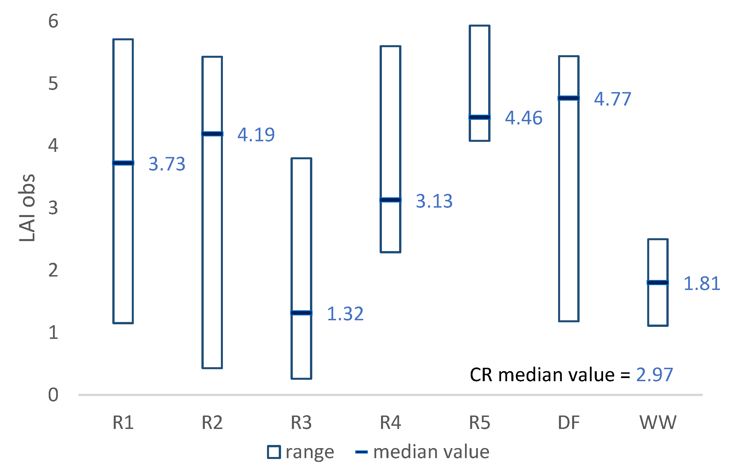
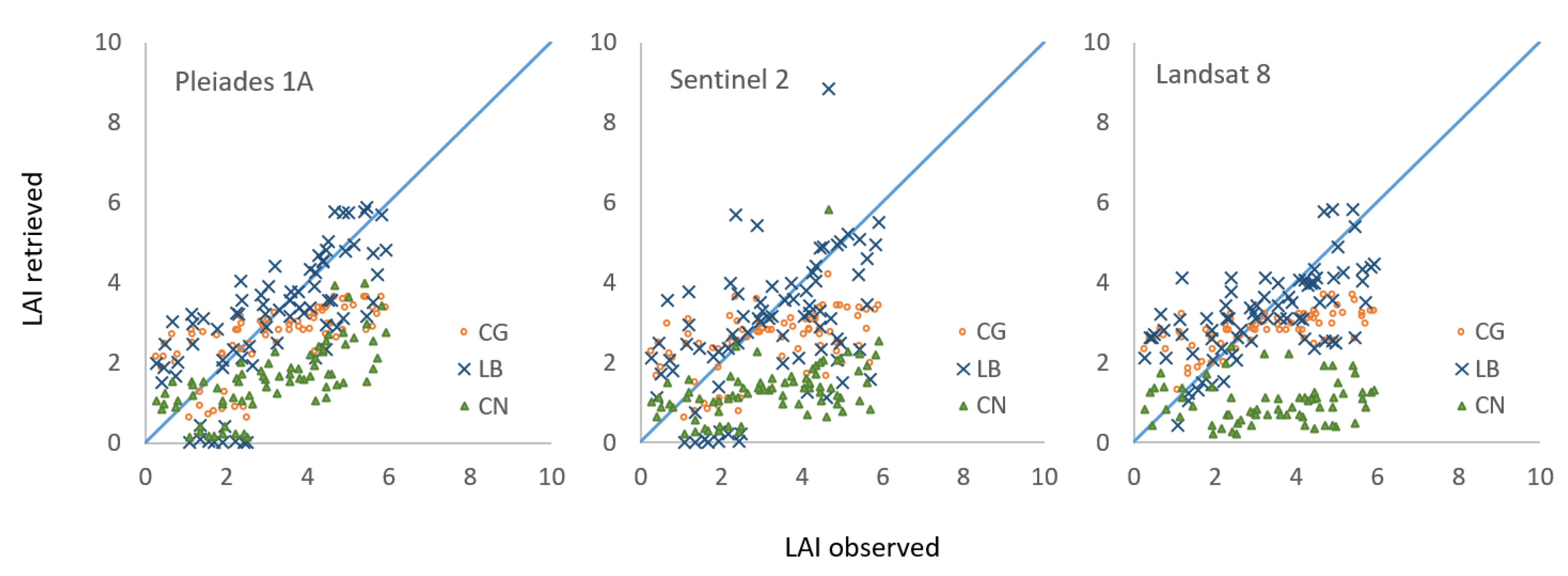
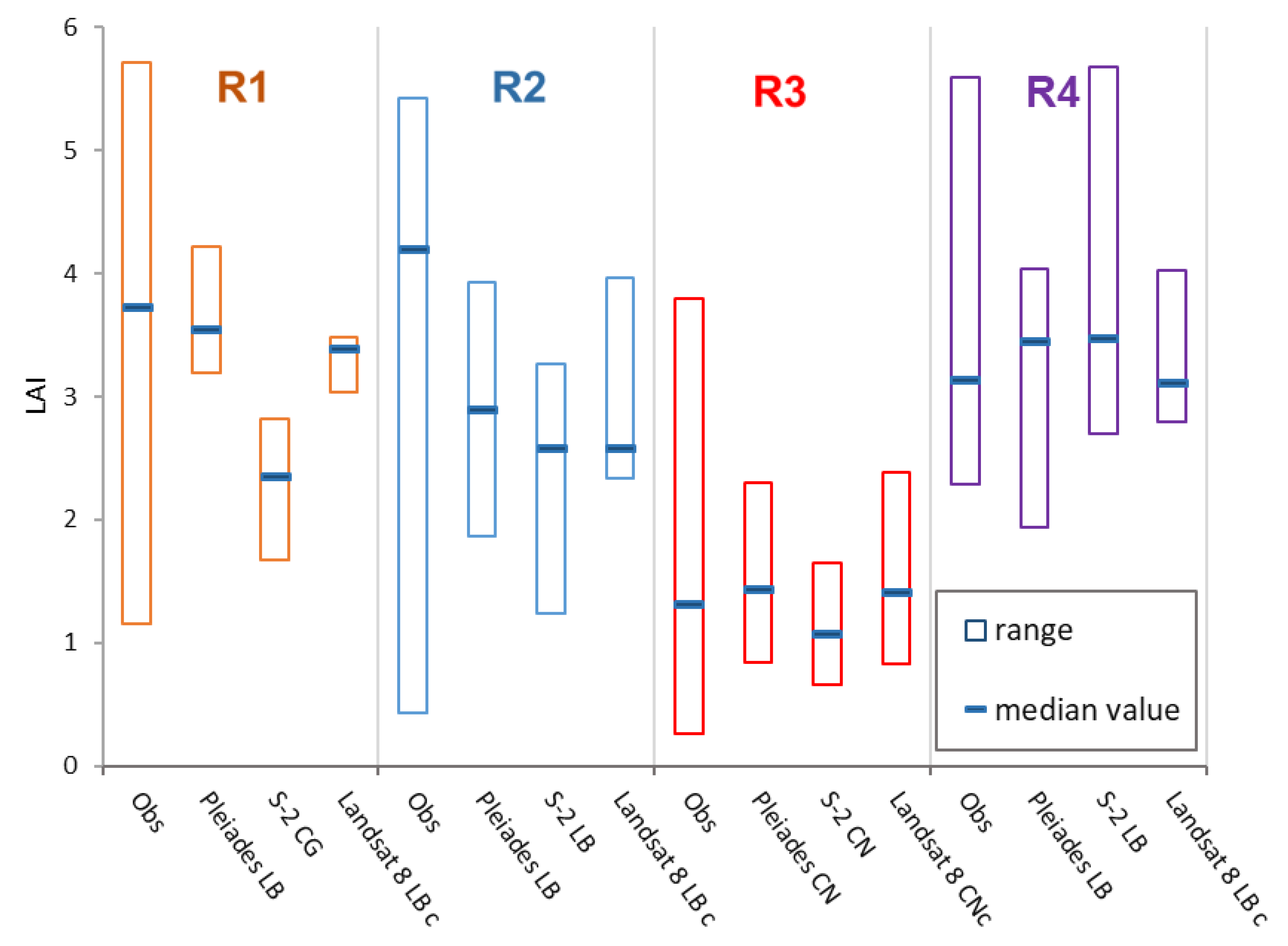
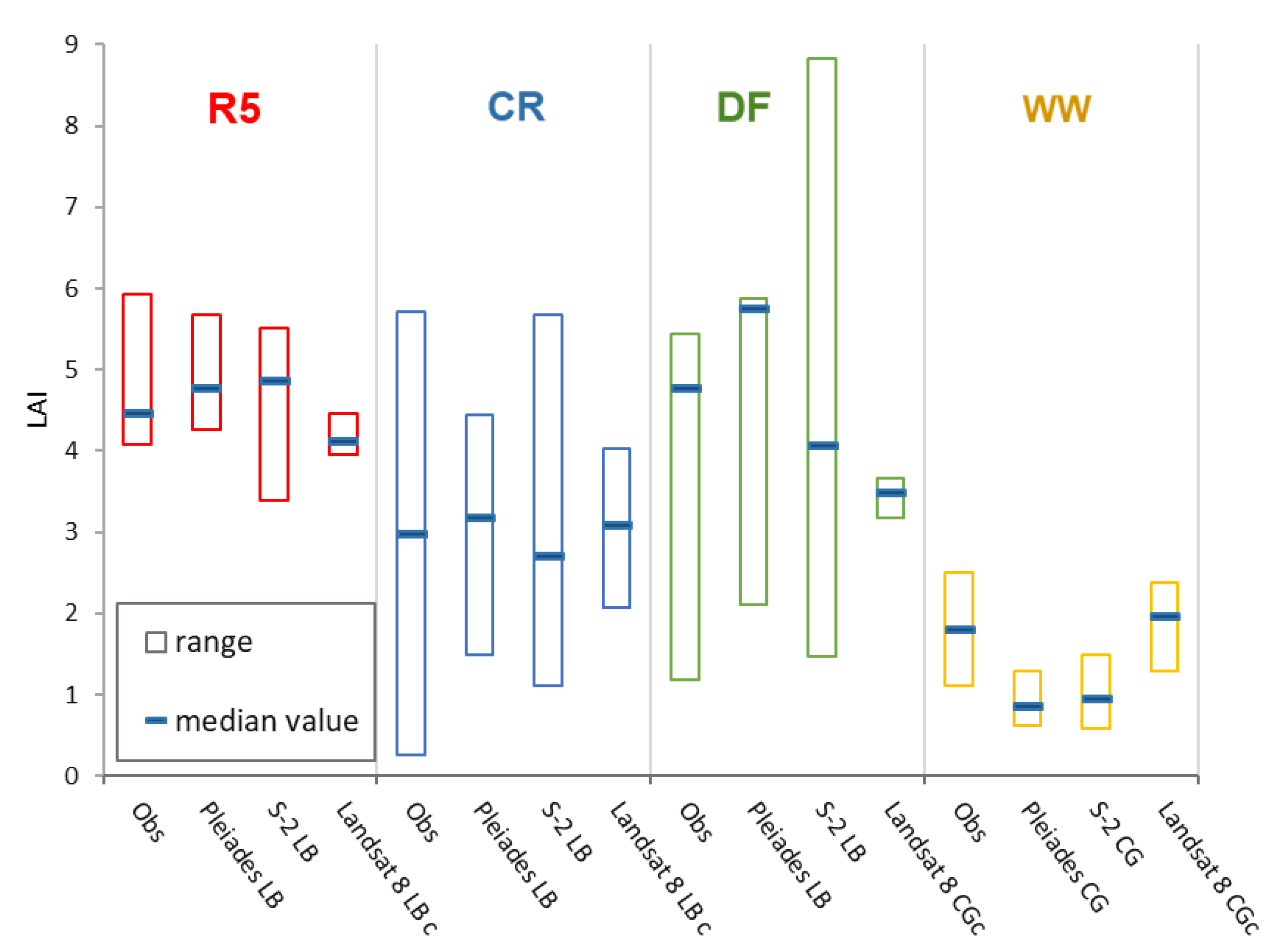
LAI values were calculated from NDVI data retrieved from the three selected satellite images using the following Equation (1) [59]:
N D V I   =   N I R R e d N I R + R e d
In the case of L8 imagery, the corrected Normalized Difference Vegetation Index (NDVIc) was calculated to improve the correlation accuracy between the NDVI and LAI. The NDVIc uses the mid-infrared band as a filter to eliminate or reduce the contribution of ground vegetation and yields more accurate canopy values [60]. Although the correction was also tested for S-2, it was not applied because it yielded very low NDVI, probably due to differences in band wavelengths with respect to L8 [61]. Moreover, the correction was not performed for P1A data, due to the lack of information in the shortwave infrared band [62].
LAI values were then calculated using the following three equations (Table 2): Caraux-Garson (CG, [63]), Lambert-Beer (LB, [64]), and Campbell and Norman (CN, [65]). The accuracy of the results was assessed using the PBIAS (percent bias, [66]), R2 (coefficient of determination, [67]), and NSE (Nash–Sutcliffe efficiency index, [68] statistical indices.

3. Results

The observed LAIs (LAIobs) differed significantly at the monitored sites, both in range and median value (Figure 3). Overall, LAIobs values along RV transects ranged from 0.26 to 5.93. In particular, CR showed a variation of 5.45 (0.26–5.71 range) and a median value of 2.97. The lower LAI values were mostly found in R2 and R3, the higher ones in R1, R2, and R4. In contrast, more uniform LAI values were detected in R5, where the variation was only 1.85 (4.08–5.93 range), and the median was 4.46.
The higher LAI values detected in R5 were comparable to those obtained in R1, R2, and R3 of the CR (Figure 3).
As expected, WW showed the narrowest range of LAIobs (1.11–2.50) and the lowest median value (1.81). However, values detected in WW are similar to the lower values measured in R2 and R3. The variability of LAIobs values in DF was 4.26 (1.18–5.44 range). Although this, the median, was in absolute the highest detected (4.77), which was very similar to the median obtained in R5. Moreover, the higher DF values were comparable to the higher LAIobs in R1, R2, and R3.
The PBIAS (percent bias), R2 (coefficient of determination), and NSE (Nash–Sutcliffe efficiency index) statistical indices were used to assess the accuracy of LAI values calculated based on NDVI values derived from the different remote sensing images (Landsat 8, Sentinel-2, and Pleiades 1A) using Equations (a)–(c). This analysis was carried out considering the different types of vegetation monitored (riparian vegetation, deciduous forest, and winter wheat fields). In particular, to determine which combination of image and equation is most suited to the study of variability in riparian vegetation, the performance was evaluated for every single reach (R1–R5) of RV. The results are reported in Table 3.
On the whole, all three satellite images underestimated LAIobs (PBIAS > 0) in R1. The equation which yielded the best accuracy was LB for L8 and P1A and CG for S-2. In particular, L8 and P1A performed comparably well, with a slightly finer accuracy for P1A (lower RMSE) and better than S-2. The extreme variability of LAIs measured in R2 (the incipient erosion reach) was not detected correctly by any imagery and was generally underestimated. In any case, LB is the equation that performed best for all the satellite platforms. L8, followed by P1A and S-2, when processed with equation CN, yielded the best results in R3. In particular, LAIobs values were slightly overestimated by L8 (PBIAS < 0) and underestimated by P1A and S-2. L8 and equation LB, gave the best results in R4. In this case, the calculated values slightly underestimated the LAIobs. In R5, the last reach of RV, P1A performed best, with slight overestimation. S–2 and L8, instead, tended to underestimate the LAIobs. Here, equation LB yielded the best results for all the satellite platforms. Considering the other two vegetation types, P1A showed the best statistical indices, followed by L8 and S-2 in DF, when all processed with LB. In general, all the images overestimated LAIobs values. In WW, both P1A and S-2 performed poorly, greatly underestimating the LAIobs. L8 performed better statistically, although LAI values were slightly overestimated. Equation CG worked best.
Figure 4 represents the scatterplots between LAIobs and LAI retrieved values for each satellite imagery, which give a visual assessment of the validation results reported in Table 3. The plots confirm a good prediction ability for the LB equation, except for WW in P1A and S-2, while showing a tendency to underestimate LAI values for the CN and CG equations.
For comparison. The ranges and median values of both LAIobs and LAI derived from all three satellite images (Landsat 8, Sentinel-2, and Pleiades 1A) were plotted using the equation that best suited each type of vegetation (Table 3), (Figure 5 and Figure 6).
LAIobs values generally showed wider ranges than LAI retrieved from satellite imagery, especially in the reaches of the CR. None of the three satellite images detected the high variability of the LAIobs in R1, R2, and R3. In R4, S-2 yielded a value range very similar to that of LAIobs; in particular, the highest LAIobs and calculated LAI values were 5.60 and 5.68, respectively, whereas the lowest were 2.29 and 2.70, respectively (Figure 5). S-2 also detected ranges well in R5, although with a tendency to underestimate both higher and lower LAI values (Figure 6). In this reach, P1A yielded a more accurate minimum (4.08, LAIobs and 4.27, LAI retrieved) and maximum (5.93, LAIobs and 5.68, LAI retrieved) values (Figure 6). P1A also accurately detected LAI variability in DF. The ranges were quite similar (4.26 for LAIobs and 3.75 for retrieved LAI), although retrieved LAI values slightly overestimated both the lower and higher values (Figure 6). WW was the only land use category in which L8 performed best in terms of both lower and higher values (Figure 6). However, the maximum value was underestimated (2.50 for LAIobs and 2.37 for retrieved LAI). P1A and L8 median values (3.54 and 3.39, respectively) were close to the observed one (3.73) in R1 (Figure 5). In R2, instead, none of the satellite platforms considered yielded median LAI values in good agreement with the median LAIobs (Figure 5). In R3, both L8 and P1A yielded median LAI values (1.41 and 1.43, respectively) similar to the LAIobs (1.32) (Figure 5). S-2 also yielded accurate results, although the median LAI retrieved was underestimated (1.06). In R4, the median LAIobs was 3.13. L8 yielded the best results (3.10), whereas P1A and S-2 tended to overestimate actual values (3.37 and 3.50, respectively) (Figure 5). In R5, where the median LAIobs was 4.46, P1A yielded the most accurate results (4.76), followed by L8 (4.12) and S-2 (4.86). As for the two other types of vegetation cover, DF and WW, only L8 yielded a median value comparable to the observed value. In DF, LAIobs was 4.77, and the retrieved LAI was 5.14 (Figure 6); whereas, in WW, the LAIobs was 1.81, and the retrieved LAI was 1.97 (Figure 6).

4. Discussion

The LAI of RV was measured in-situ (LAI 2200 Plant Canopy Analyzer) and retrieved from satellite imagery to test the performance of three satellite images with different spatial resolutions (Pleiades 1-A, Sentinel-2, and Landsat 8). DF and WW land cover types were also analyzed to compare results with those obtained for RV. As the NDVI is one of the Vis most commonly used to detect canopy cover variability [31], the LAI-NDVI approach was used to derive LAI values using three different equations (Lambert-Beer, Caraux-Garson, and Campbell-Norman).
The wide variability of in-field LAIobs measurements for RV reflects the composition and structure of such complex environments. In particular, in R2 and in R3, characterized, respectively, by partially or totally destroyed check dams, LAIobs values were lower, highlighting a correlation between the vegetation status and geomorphological channel stability [12,38,69]. R1 and R4, where there is almost no erosion and vegetation is more stratified, showed a higher maximum LAIobs comparable to the values measured in the DF. R5, characterized by intact check dams and well-structured riparian vegetation, has median LAIobs values similar to those detected in R4. Higher values are detected in DF because the vegetation here is mostly single story, without the presence of ground vegetation. As expected, LAIobs values for the WW field are low and show less variability, due to the unstratified cover and the simple leaf structure.
As for the performance of the three satellite images in the study area, L8 and P1A showed similar results in R1, R3, R4, R5, and DF. Where erosion processes influence the presence of vegetation (R3), P1A and L8 yielded very similar ranges and median values. In R1 and R4, instead, although statistical values were similar between L8 and P1A, there was a better match between value ranges for P1A.
In R5 and DF, the better statistical performance of P1A was due to the high-resolution, which limited the negative influence of “mixed pixels” [70,71], which instead affected L8 [27] (Figure 6), as well as S-2, whose image resolution (10 m) was too coarse to avoid the “mixed pixels” effect. In R4 and WW, instead, L8 performed better than P1A. In Figure 5 and Figure 6, LAIobs and retrieved LAI show a better match in terms of median values for both R4 and WW, and the best match of value ranges for WW. In both cases, P1A underestimated LAI, especially the lower range values.
The reason why P1A show no noticeable improvements with respect to L8, especially considering R4 and WW, may be due to the different satellite data acquisition period (1 June and 3 July for L8, 20 July for P1A). Satellite imagery are sensible to biological factors [72], such as the phenological phases of vegetation [73], and imagery acquired at the right time for the purposes of a study can yield better results, even with images at a coarser scale [74]. At the end of July, the herbaceous plants characterizing R4 riverbed vegetation were in a water stress phase, and all crops had been harvested in the WW fields. Moreover, although the higher spatial resolution, P1A is characterized by a lower spectral resolution with respect to L8 and S-2 (4 bands in P1A) [53]. This means that the P1A red and NIR bandwidth are greater respect to the same bands of L8 and S-2. Teillet et al. [75] demonstrated that an increase in the bandwidth is directly related to a decrease in the values of the NDVI.
In general, the statistical performances of S-2 were worse than those of the other sensors, except for R5, where it performed comparably to L8 and P1A, while it was the only image to capture the extreme variability of LAIobs values in CR and R5 (Figure 5 and Figure 6). The worse statistical performances of S-2 could depend on several factors. First, as mentioned above, the acquisition date (28 July) certainly influences the accuracy of results [74]. Moreover, several authors [76,77,78] highlight that although NDVI is commonly used to retrieve LAI values, it is not always the VI with the highest correlation. In particular, for S-2, the newest of the three satellites, alternative Vis may be considered to improve results [32,79,80,81].
None of the sensors was a good descriptor of the high variability of LAIobs values in R2, resulting in a general underestimation. In this reach, where the vegetation was sparse or totally absent [27], L8 and S-2 were affected by the “mixed pixel” effect [71]. P1A, which is characterized by a lower spectral resolution, and consequently, by higher bandwidth, suffered a spectral interference of the soil background, due to the surface heterogeneity [82,83].
As regards the use of different equations to derive LAI from the NDVI, results indicate that, in almost all cases, the Lambert-Beer (LB) equation was the most suitable. In particular, when the vegetation was more homogenous (R1, R4, R5, and DF), LB worked best in processing both the L8 and the P1A imagery. Moreover, LB (coupled with P1A) improved the results in R2, although with unsatisfactory statistics, confirming that the more complex features in R2 are not easily detected using satellite imagery (Romano et al., 2020). However, it should be considered that at each specific site, there may be variations related to canopy characteristics (i.e., density, leaf angle distribution) and soil optical properties [84,85]. For this reason, the match between the LAIobs and retrieved LAI could still be improved by modifying the De Jong coefficients [86], generic for Mediterranean areas, used in the LB equation. In R3, confirming findings by Ricci et al. [27] for L8, the equation CN performed well also in processing S-2 and P1A. This equation requires identifying two NDVI values representing the value of bare soil and the maximum value for vegetation [65]. In a complex environment, such as a Mediterranean watershed that includes different types of vegetation, the first value is easy to determine, whereas the second is difficult to determine because the maximum value of the vegetation depends, within the same image, on changes in vegetation type [87,88]. For this reason, CN yielded acceptable results in R3 only, where only LAIobs values similar to those of the bare soil were estimated correctly (Figure 5). Linear equation CG yielded the best accuracy for WW because, where the observed LAI values were lower than 3, results were not affected by the effect of saturation on greenness, which for higher values determines an asymptotic trend in retrieved LAIs [31,85]. Generally, differences in results could also be ascribed to the fact that the adopted equations were developed before the launch of both the P1A and the S-2 missions, so that the correlation coefficients may not be optimal. In addition, since LAIobs measurements are required to validate retrieved data, the sampling design is an important aspect to consider [89]. In this work, transects were selected to obtain the most suitable overlap between field measurements and the spatial resolutions of satellite images. For this reason, P1A results could be improved using a different sampling design for medium resolution imagery (L8 and S-2) and high-resolution imagery (P1A). The obtained results, confirm what was observed by Wang et al. [53], or that the spatial resolution is an important factor to consider when choosing a satellite product, but to the differences in the satellite sensors bands (spectral resolution) could also impact the results.

5. Conclusions

This study assessed the potential of three satellite images with different resolutions (Landsat 8, Sentinel-2, and Pleiades 1A) in studying vegetation features in a mountain riparian environment of Southern Italy. Pleiades 1A and Landsat 8 imagery yielded values closer to the observed ones. In particular, the higher spatial resolution of the former limited the influence of the mixed pixel over the study area and improved the results both in terms of statistics and retrieved LAI value ranges. However, the lower spectral resolution of the Pleiades 1A leads to spectral interference, due to the surface heterogeneity, and to an underestimation of the results, especially in the transects where the vegetation is variable. Sentinel-2 imagery showed poor statistical performances attributable, mainly, to both the acquisition date of the image and to the vegetation index considered, which may not be the best for this type of sensor. The results obtained suggest that, apart from the spatial resolution, other factors have an impact on the LAI retrieval. The spectral resolution could negatively influence the results, especially when the environment is more complex. The time of acquisition should be as close as possible to the in-field measurement period, since the satellite multispectral images are sensitive to the phenology of vegetation. The sampling design could improve the accuracy of the results if it is specifically designed for the satellite sensor. A cost analysis is another key issue, as some remote sensing images can be downloaded free of charge (i.e., Landsat 8 and Sentinel 2), while others cannot (i.e., Pleiades 1A). Future studies could aim to improve the coefficient of the Lambert-Beer equation for the Mediterranean areas, and/or test the performance of different vegetation indices—especially for the Sentinel-2 imagery.

Author Contributions

Conceptualization: G.F.R., G.R. and F.G.; Methodology: G.F.R., G.R. and F.G. Investigation: G.F.R., G.R.; Writing—original draft preparation: G.F.R., G.R.; Writing—review and editing: G.F.R., G.R. and F.G.; Project administration: F.G.; Funding: F.G. All authors have read and agreed to the published version of the manuscript.

Funding

The Pleiades acquisition was founded by Fondazione Cassa di Risparmio di Puglia, Project “Impiego delle immagini da satellite nella gestione della risorsa idrica a scala di bacino”, Scientific Coordinator prof. Francesco Gentile, University of Bari.

Acknowledgments

The authors wish to thank Francesco Urgesi and Francesco Scognamiglio for their contributions during the field monitoring activity.

Conflicts of Interest

The authors declare no conflict of interest.

References

  1. Horning, N. Remote Sensing. In Encyclopedia of Ecology; Elsevier: Amsterdam, The Netherlands, 2008. [Google Scholar]
  2. Slonecker, E.T.; Jennings, D.B.; Garofalo, D. Remote sensing of impervious surfaces: A review. Remote Sens. Rev. 2001, 20, 227–255. [Google Scholar] [CrossRef]
  3. Balsamo, G.; Agusti-Panareda, A.; Albergel, C.; Arduini, G.; Beljaars, A.; Bidlot, J.; Blyth, E.; Bousserez, N.; Boussetta, S.; Brown, A.; et al. Satellite and In Situ Observations for Advancing Global Earth Surface Modelling: A Review. Remote Sens. 2018, 10, 2038. [Google Scholar] [CrossRef] [Green Version]
  4. Schowengerdt, R.A. Remote Sensing; Elsevier: Amsterdam, The Netherlands, 2007; ISBN 9780123694072. [Google Scholar]
  5. Salamí, E.; Barrado, C.; Pastor, E. UAV Flight Experiments Applied to the Remote Sensing of Vegetated Areas. Remote Sens. 2014, 6, 11051–11081. [Google Scholar] [CrossRef] [Green Version]
  6. Räsänen, A.; Virtanen, T. Data and resolution requirements in mapping vegetation in spatially heterogeneous landscapes. Remote Sens. Environ. 2019, 230, 111207. [Google Scholar] [CrossRef]
  7. Yao, H.; Qin, R.; Chen, X. Unmanned Aerial Vehicle for Remote Sensing Applications—A Review. Remote Sens. 2019, 11, 1443. [Google Scholar] [CrossRef] [Green Version]
  8. Calsamiglia, A.; Gago, J.; Garcia-Comendador, J.; Bernat, J.F.; Calvo-Cases, A.; Estrany, J. Evaluating functional connectivity in a small agricultural catchment under contrasting flood events by using UAV. Earth Surf. Process. Landf. 2020, 45, 800–815. [Google Scholar] [CrossRef]
  9. Matese, A.; Toscano, P.; Di Gennaro, S.; Genesio, L.; Vaccari, F.; Primicerio, J.; Belli, C.; Zaldei, A.; Bianconi, R.; Gioli, B. Intercomparison of UAV, Aircraft and Satellite Remote Sensing Platforms for Precision Viticulture. Remote Sens. 2015, 7, 2971–2990. [Google Scholar] [CrossRef] [Green Version]
  10. Chen, Y.; Guerschman, J.P.; Cheng, Z.; Guo, L. Remote sensing for vegetation monitoring in carbon capture storage regions: A review. Appl. Energy 2019, 240, 312–326. [Google Scholar] [CrossRef]
  11. Xue, J.; Su, B. Significant remote sensing vegetation indices: A review of developments and applications. J. Sens. 2017, 2017, 1353691. [Google Scholar] [CrossRef] [Green Version]
  12. Romano, G.; Ricci, G.F.; Gentile, F. Comparing LAI Field Measurements and Remote Sensing to Assess the Influence of Check Dams on Riparian Vegetation Cover. In Lecture Notes in Civil Engineering; Coppola, A., Di Renzo, G., Altieri, G., D’Antonio, P., Eds.; Springer: Berlin, Germany, 2020; Volume 67, pp. 109–116. [Google Scholar]
  13. Liang, S.; Wang, J. Advanced Remote Sensing Terrestrial Information Extraction and Applications, 2nd ed.; Elsevier: Amsterdam, The Netherlands, 2020. [Google Scholar]
  14. Vorovencii, L. Satellite Remote Sensing in Environmental Impact Assessment: An Overview. Bull. Transilv. Univ. Braşov 2011, 4, 1–8. [Google Scholar]
  15. Toth, C.; Jóźków, G. Remote sensing platforms and sensors: A survey. ISPRS J. Photogramm. Remote Sens. 2016, 115, 22–36. [Google Scholar] [CrossRef]
  16. Piermattei, L.; Marty, M.; Karel, W.; Ressl, C.; Hollaus, M.; Ginzler, C.; Pfeifer, N. Impact of the Acquisition Geometry of Very High-Resolution Pléiades Imagery on the Accuracy of Canopy Height Models over Forested Alpine Regions. Remote Sens. 2018, 10, 1542. [Google Scholar] [CrossRef] [Green Version]
  17. Johansen, K.; Coops, N.C.; Gergel, S.E.; Stange, Y. Application of high spatial resolution satellite imagery for riparian and forest ecosystem classification. Remote Sens. Environ. 2007, 110, 29–44. [Google Scholar] [CrossRef]
  18. Lopez, R.R.D.; Frohn, R.C. Remote Sensing for Landscape Ecology: New Metric Indicators: Monitoring, Modeling, and Assessment of Ecosystems, 2nd ed.; CRC Press: Boca Raton, FL, USA, 2017; ISBN 9781498754392. [Google Scholar]
  19. Lu, D. The potential and challenge of remote sensing-based biomass estimation. Int. J. Remote Sens. 2006, 27, 1297–1328. [Google Scholar] [CrossRef]
  20. Lu, D.; Chen, Q.; Wang, G.; Liu, L.; Li, G.; Moran, E. A survey of remote sensing-based aboveground biomass estimation methods in forest ecosystems. Int. J. Digit. Earth 2016, 9, 63–105. [Google Scholar] [CrossRef]
  21. Chen, J.M.; Black, T.A. Defining leaf area index for non-flat leaves. Plant. Cell Environ. 1992, 15, 421–429. [Google Scholar] [CrossRef]
  22. Nagler, P.L.; Glenn, E.P.; Huete, A.R. Assessment of spectral vegetation indices for riparian vegetation in the Colorado River delta, Mexico. J. Arid Environ. 2001, 49, 91–110. [Google Scholar] [CrossRef]
  23. Pierce, L.L.; Running, S.W. Rapid estimation of coniferous forest leaf area index using a portable integrating radiometer. Ecology 1988, 69, 1762–1767. [Google Scholar] [CrossRef]
  24. Fang, H.; Liang, S. Leaf Area Index Models. In Reference Module in Earth Systems and Environmental Sciences; Elsevier: Amsterdam, The Netherlands, 2014. [Google Scholar]
  25. McMichael, C.E.; Hope, A.S.; Roberts, D.A.; Anaya, M.R. Post-fire recovery of leaf area index in California chaparral: A remote sensing-chronosequence approach. Int. J. Remote Sens. 2004, 25, 4743–4760. [Google Scholar] [CrossRef]
  26. Chapin, F.S.; Eviner, V.T. Biogeochemistry of Terrestrial Net Primary Production. In Treatise on Geochemistry; Elsevier: Amsterdam, The Netherlands, 2007; Volumes 8–9, pp. 1–35. ISBN 9780080548074. [Google Scholar]
  27. Ricci, G.F.; Romano, G.; Leronni, V.; Gentile, F. Effect of check dams on riparian vegetation cover: A multiscale approach based on field measurements and satellite images for Leaf Area Index assessment. Sci. Total Environ. 2019, 657, 827–838. [Google Scholar] [CrossRef]
  28. Richards, D.; Wang, J.W. Fusing street level photographs and satellite remote sensing to map leaf area index. Ecol. Indic. 2020, 115. [Google Scholar] [CrossRef]
  29. Wang, Q.; Adiku, S.; Tenhunen, J.; Granier, A. On the relationship of NDVI with leaf area index in a deciduous forest site. Remote Sens. Environ. 2005, 94, 244–255. [Google Scholar] [CrossRef]
  30. Sripada, R.P.; Heiniger, R.W.; White, J.G.; Weisz, R. Aerial Color Infrared Photography for Determining Late-Season Nitrogen Requirements in Corn. Reprod. Agron. J. 2005, 98, 968–977. [Google Scholar] [CrossRef]
  31. Milella, P.; Bisantino, T.; Gentile, F.; Iacobellis, V.; Trisorio Liuzzi, G. Diagnostic analysis of distributed input and parameter datasets in Mediterranean basin streamflow modeling. J. Hydrol. 2012, 472–473, 262–276. [Google Scholar] [CrossRef]
  32. Sinha, S.K.; Padalia, H.; Dasgupta, A.; Verrelst, J.; Rivera, J.P. Estimation of leaf area index using PROSAIL based LUT inversion, MLRA-GPR and empirical models: Case study of tropical deciduous forest plantation, North India. Int. J. Appl. Earth Obs. Geoinf. 2020, 86, 102027. [Google Scholar] [CrossRef]
  33. Xavier, A.C.; Vettorazzi, C.A. Mapping leaf area index through spectral vegetation indices in a subtropical watershed. Int. J. Remote Sens. 2004, 25, 1661–1672. [Google Scholar] [CrossRef]
  34. Malanson, G.P. Riparian Landscapes; Cambridge University Press: Cambridge, UK, 1993. [Google Scholar]
  35. Hancock, C.N.; Ladd, P.G.; Froend, R.H. Biodiversity and management of riparian vegetation in western Australia. For. Ecol. Manag. 1996, 85, 239–250. [Google Scholar] [CrossRef]
  36. Inoue, M.; Nakagoshi, N. The effects of human impact on spatial structure of the riparian vegetation along the Ashida river, Japan. Landsc. Urban Plan. 2001, 53, 111–121. [Google Scholar] [CrossRef]
  37. Fu, B.; Li, Y.; Wang, Y.; Zhang, B.; Yin, S.; Zhu, H.; Xing, Z. Evaluation of ecosystem service value of riparian zone using land use data from 1986 to 2012. Ecol. Indic. 2016, 69, 873–881. [Google Scholar] [CrossRef]
  38. Bombino, G.; Boix-Fayos, C.; Gurnell, A.M.; Tamburino, V.; Zema, D.A.; Zimbone, S.M. Check dam influence on vegetation species diversity in mountain torrents of the Mediterranean environment. Ecohydrology 2014, 7, 678–691. [Google Scholar] [CrossRef]
  39. Zema, D.A.; Bombino, G.; Denisi, P.; Lucas-Borja, M.E.; Zimbone, S.M. Evaluating the effects of check dams on channel geometry, bed sediment size and riparian vegetation in Mediterranean mountain torrents. Sci. Total Environ. 2018, 642, 327–340. [Google Scholar] [CrossRef]
  40. Vigiak, O.; Malagó, A.; Bouraoui, F.; Grizzetti, B.; Weissteiner, C.J.; Pastori, M. Impact of current riparian land on sediment retention in the Danube River Basin. Sustain. Water Qual. Ecol. 2016, 8, 30–49. [Google Scholar] [CrossRef]
  41. European Commission Directive 2000/60/EC. Official Journal of the European Communities. 2000. Available online: https://eur-lex.europa.eu/legal-content/EN/TXT/?uri=celex:32000L0060 (accessed on 8 September 2020).
  42. Stella, J.C.; Rodríguez-González, P.M.; Dufour, S.; Bendix, J. Riparian vegetation research in Mediterranean-climate regions: Common patterns, ecological processes, and considerations for management. Hydrobiologia 2013, 719, 291–315. [Google Scholar] [CrossRef]
  43. Clerici, N.; Weissteiner, C.J.; Paracchini, M.L.; Boschetti, L.; Baraldi, A.; Strobl, P. Pan-European distribution modelling of stream riparian zones based on multi-source Earth Observation data. Ecol. Indic. 2013, 24, 211–223. [Google Scholar] [CrossRef]
  44. LI-COR LI-2200C Plant Canopy Analyzer. 2010. Available online: https://licor.app.boxenterprise.net/s/fqjn5mlu8c1a7zir5qel (accessed on 8 September 2020).
  45. Abdelwahab, O.M.M.; Bingner, R.L.; Milillo, F.; Gentile, F. Evaluation of Alternative Management Practices with the AnnAGNPS Model in the Carapelle Watershed. Soil Sci. 2016, 181, 293–305. [Google Scholar] [CrossRef]
  46. Bisantino, T.; Gentile, F.; Milella, P.; Liuzzi, G.T. Effect of Time Scale on the Performance of Different Sediment Transport Formulas in a Semiarid Region. J. Hydraul. Eng. 2010, 136, 56–61. [Google Scholar] [CrossRef]
  47. Ricci, G.F.; De Girolamo, A.M.; Abdelwahab, O.M.M.; Gentile, F. Identifying sediment source areas in a Mediterranean watershed using the SWAT model. Land Degrad. Dev. 2018, 29, 1233–1248. [Google Scholar] [CrossRef]
  48. Aquilino, M.; Novelli, A.; Tarantino, E.; Iacobellis, V.; Gentile, F. Evaluating the Potential of GeoEye Data in Retrieving LAI at Watershed Scale. In Remote Sensing for Agriculture, Ecosystems, and Hydrology XVI, Proceedings of the SPIE Remote Sensing, Amsterdam, The Netherlands, 22–25 September 2014; Neale, C.M.U., Maltese, A., Eds.; SPIE: Paris, France, 2014; Volume 9239, p. 92392B. [Google Scholar]
  49. Yan, G.; Hu, R.; Luo, J.; Weiss, M.; Jiang, H.; Mu, X.; Xie, D.; Zhang, W. Review of indirect optical measurements of leaf area index: Recent advances, challenges, and perspectives. Agric. For. Meteorol. 2019, 265, 390–411. [Google Scholar] [CrossRef]
  50. Riihimäki, H.; Luoto, M.; Heiskanen, J. Estimating fractional cover of tundra vegetation at multiple scales using unmanned aerial systems and optical satellite data. Remote Sens. Environ. 2019, 224, 119–132. [Google Scholar] [CrossRef]
  51. Mihai, B.A.; Săvulescu, I.; Vîrghileanu, M.; Olariu, B. Evaluation of sentinel-2 MSI and pleiades 1B imagery in forest fire susceptibility assessment in temperate regions of Central and Eastern Europe. A Case study of Romania. In Advances in Natural and Technological Hazards Research; Springer: Rotterdam, The Netherlands, 2019; Volume 48, pp. 253–269. [Google Scholar]
  52. Pu, R.; Landry, S. Evaluating seasonal effect on forest leaf area index mapping using multi-seasonal high resolution satellite pléiades imagery. Int. J. Appl. Earth Obs. Geoinf. 2019, 80, 268–279. [Google Scholar] [CrossRef]
  53. Wang, D.; Wan, B.; Qiu, P.; Su, Y.; Guo, Q.; Wang, R.; Sun, F.; Wu, X. Evaluating the Performance of Sentinel-2, Landsat 8 and Pléiades-1 in Mapping Mangrove Extent and Species. Remote Sens. 2018, 10, 1468. [Google Scholar] [CrossRef] [Green Version]
  54. Chander, G.; Markham, B.L.; Helder, D.L. Summary of current radiometric calibration coefficients for Landsat MSS, TM, ETM+, and EO-1 ALI sensors. Remote Sens. Environ. 2009, 113, 893–903. [Google Scholar] [CrossRef]
  55. Romano, G.; Abdelwahab, O.M.M.; Gentile, F. Modeling land use changes and their impact on sediment load in a Mediterranean watershed. Catena 2018, 163, 342–353. [Google Scholar] [CrossRef]
  56. Vanhellemont, Q.; Ruddick, K. Atmospheric correction of metre-scale optical satellite data for inland and coastal water applications. Remote Sens. Environ. 2018, 216, 586–597. [Google Scholar] [CrossRef]
  57. Zhan, Z.-Z.; Liu, H.-B.; Li, H.-M.; Wu, W.; Zhong, B. The Relationship between NDVI and Terrain Factors—A Case Study of Chongqing. Procedia Environ. Sci. 2012, 12, 765–771. [Google Scholar] [CrossRef] [Green Version]
  58. Ayalew, D.A.; Deumlich, D.; Šarapatka, B.; Doktor, D. Quantifying the Sensitivity of NDVI-Based C Factor Estimation and Potential Soil Erosion Prediction using Spaceborne Earth Observation Data. Remote Sens. 2020, 12, 1136. [Google Scholar] [CrossRef] [Green Version]
  59. Rouse, J.W.J.; Haas, R.; Schell, J.; Deering, D.; Harlan, J.C. Monitoring the Vernal Advancement and Retrogradation (Green Wave Effect) of Natural Vegetation. Available online: https://ntrs.nasa.gov/citations/19740008955 (accessed on 12 September 2020).
  60. Nemani, R.; Pierce, L.; Running, S.; Band, L. Forest ecosystem processes at the watershed scale: Sensitivity to remotely-sensed leaf area index estimates. Int. J. Remote Sens. 1993, 14, 2519–2534. [Google Scholar] [CrossRef]
  61. Sibanda, M.; Mutanga, O.; Rouget, M. Examining the potential of Sentinel-2 MSI spectral resolution in quantifying above ground biomass across different fertilizer treatments. ISPRS J. Photogramm. Remote Sens. 2015, 110, 55–65. [Google Scholar] [CrossRef]
  62. Cahalane, C.; Magee, A.; Monteys, X.; Casal, G.; Hanafin, J.; Harris, P. A comparison of Landsat 8, RapidEye and Pleiades products for improving empirical predictions of satellite-derived bathymetry. Remote Sens. Environ. 2019, 233, 111414. [Google Scholar] [CrossRef]
  63. Caraux-Garson, D.; Lacaze, B.; Scala, F.; Hill, J.; Mehel, W. Ten years of vegetation cover monitoring with Landsat TM remote sensing, an operational approach of DeMon-2 in Languedoc, France. In Proceedings of the 18th EARSeL Symposium on Operational Remote Sensing for Sustainable Development, Enschede, The Netherlands, 11–14 May 1998. [Google Scholar]
  64. Lacaze, B. Integrated Approaches to Desertification Mapping and Monitoring in the Mediterranean Basin: Final Report of the DEMON-1 Project; Space Applications Institute, Environmental Mapping and Modelling Unit: Ahmedabad, India, 1996. [Google Scholar]
  65. Walthall, C.L.; Dulaney, W.P.; Anderson, M.C.; Norman, J.; Fang, H.; Liang, S.; Timlin, D.J.; Pachepsky, Y. Alternative Approaches for Estimating Leaf Area Index (LAI) from Remotely Sensed Satellite and Aircraft Imagery. In Remote Sensing and Modeling of Ecosystems for Sustainability, Proceedings of the Optical Science And Technology, The Spie 49th Annual Meeting, Denver, CO, USA, 2–6 August 2004; Gao, W., Shaw, D.R., Eds.; SPIE: Paris, France, 2004; Volume 5544, p. 241. [Google Scholar]
  66. Wiant, H.V.; Harner, E.J. Percent Bias and Standard Error in Logarithmic Regression. For. Sci. 1979, 25, 167–168. [Google Scholar]
  67. Wright, S. Correlation and Causation. J. Agric. Res. 1921, 20, 557–885. [Google Scholar]
  68. Nash, J.E.; Sutcliffe, J.V. River flow forecasting through conceptual models part I—A discussion of principles. J. Hydrol. 1970, 10, 282–290. [Google Scholar] [CrossRef]
  69. Ouellet, V.; Gibson, E.E.; Daniels, M.D.; Watson, N.A. Riparian and geomorphic controls on thermal habitat dynamics of pools in a temperate headwater stream. Ecohydrology 2017, 10, e1891. [Google Scholar] [CrossRef]
  70. Chen, D.; Huang, J.; Jackson, T.J. Vegetation water content estimation for corn and soybeans using spectral indices derived from MODIS near—And short-wave infrared bands. Remote Sens. Environ. 2005, 98, 225–236. [Google Scholar] [CrossRef]
  71. Lu, D.; Weng, Q. Spectral mixture analysis of the urban landscape in Indianapolis with Landsat ETM+ imagery. Photogramm. Eng. Remote Sensing 2004, 70, 1053–1062. [Google Scholar] [CrossRef]
  72. Kang, Y.; Özdoğan, M.; Zipper, S.C.; Román, M.O.; Walker, J.; Hong, S.Y.; Marshall, M.; Magliulo, V.; Moreno, J.; Alonso, L.; et al. How universal is the relationship between remotely sensed vegetation indices and crop leaf area index? A global assessment. Remote Sens. 2016, 8, 597. [Google Scholar] [CrossRef] [Green Version]
  73. Dhakar, R.; Sehgal, V.K.; Chakraborty, D.; Sahoo, R.N.; Mukherjee, J. Field scale wheat LAI retrieval from multispectral Sentinel 2A-MSI and LandSat 8-OLI imagery: Effect of atmospheric correction, image resolutions and inversion techniques. Geocarto Int. 2019, 1–21. [Google Scholar] [CrossRef]
  74. Müllerová, J.; Brůna, J.; Bartaloš, T.; Dvořák, P.; Vítková, M.; Pyšek, P. Timing Is Important: Unmanned Aircraft vs. Satellite Imagery in Plant Invasion Monitoring. Front. Plant Sci. 2017, 8, 887. [Google Scholar] [CrossRef] [Green Version]
  75. Teillet, P.M.; Staenz, K.; Williams, D.J. Effects of spectral, spatial, and radiometric characteristics on remote sensing vegetation indices of forested regions. Remote Sens. Environ. 1997, 61, 139–149. [Google Scholar] [CrossRef]
  76. Manes, F.; Anselmi, S.; Giannini, M.; Melini, S. Relationships between leaf area index (LAI) and vegetation indices to analyze and monitor Mediterranean ecosystems. In Remote Sensing for Agriculture, Ecosystems, and Hydrology II, Proceedings of the Europto Remote Sensing, Barcelona, Spain, 25–29 September 2000; Owe, M., D’Urso, G., Zilioli, E., Eds.; SPIE: Paris, France, 2001; Volume 4171, pp. 328–335. [Google Scholar]
  77. Feng, W.; Wu, Y.; He, L.; Ren, X.; Wang, Y.; Hou, G.; Wang, Y.; Liu, W.; Guo, T. An optimized non-linear vegetation index for estimating leaf area index in winter wheat. Precis. Agric. 2019, 20, 1157–1176. [Google Scholar] [CrossRef] [Green Version]
  78. Towers, P.C.; Strever, A.; Poblete-Echeverría, C. Comparison of Vegetation Indices for Leaf Area Index Estimation in Vertical Shoot Positioned Vine Canopies with and without Grenbiule Hail-Protection Netting. Remote Sens. 2019, 11, 1073. [Google Scholar] [CrossRef] [Green Version]
  79. Delegido, J.; Verrelst, J.; Alonso, L.; Moreno, J. Evaluation of sentinel-2 red-edge bands for empirical estimation of green LAI and chlorophyll content. Sensors 2011, 11, 7063–7081. [Google Scholar] [CrossRef] [PubMed] [Green Version]
  80. Clevers, J.; Kooistra, L.; van den Brande, M. Using Sentinel-2 Data for Retrieving LAI and Leaf and Canopy Chlorophyll Content of a Potato Crop. Remote Sens. 2017, 9, 405. [Google Scholar] [CrossRef] [Green Version]
  81. Pasqualotto, N.; Delegido, J.; Van Wittenberghe, S.; Rinaldi, M.; Moreno, J. Multi-Crop Green LAI Estimation with a New Simple Sentinel-2 LAI Index (SeLI). Sensors 2019, 19, 904. [Google Scholar] [CrossRef] [Green Version]
  82. Price, J.C.; Bausch, W.C. Leaf area index estimation from visible and near-infrared reflectance data. Remote Sens. Environ. 1995, 52, 55–65. [Google Scholar] [CrossRef]
  83. Mayr, M.; Samimi, C. Comparing the Dry Season In-Situ Leaf Area Index (LAI) Derived from High-Resolution RapidEye Imagery with MODIS LAI in a Namibian Savanna. Remote Sens. 2015, 7, 4834–4857. [Google Scholar] [CrossRef] [Green Version]
  84. Wu, J.; Wang, D.; Bauer, M.E. Assessing broadband vegetation indices and QuickBird data in estimating leaf area index of corn and potato canopies. F. Crop. Res. 2007, 102, 33–42. [Google Scholar] [CrossRef]
  85. Gigante, V.; Iacobellis, V.; Manfreda, S.; Milella, P.; Portoghese, I. Influences of leaf area index estimations on water balance modeling in a mediterranean semi-arid basin. Nat. Hazards Earth Syst. Sci. 2009, 9, 979–991. [Google Scholar] [CrossRef] [Green Version]
  86. De Jong, S.M. Derivation of vegetative variables from a landsat tm image for modelling soil erosion. Earth Surf. Process. Landf. 1994, 19, 165–178. [Google Scholar] [CrossRef]
  87. Hu, Z.; He, F.; Yin, J.; Lu, X.; Tang, S.; Wang, L.; Li, X. Estimation of Fractional Vegetation Cover Based on Digital Camera Survey Data and a Remote Sensing Model. J. China Univ. Min. Technol. 2007, 17, 116–120. [Google Scholar] [CrossRef]
  88. Wu, B.; Li, M.; Yan, C.; Zhou, W.; Yan, C. Developing method of vegetation fraction estimation by remote sensing for soil loss equation: A case in the Upper Basin of Miyun Reservoir. In Proceedings of the International Geoscience and Remote Sensing Symposium (IGARSS), Anchorage, AK, USA, 20–24 September 2004; Volume 6, pp. 4352–4355. [Google Scholar]
  89. Mu, X.; Hu, M.; Song, W.; Ruan, G.; Ge, Y.; Wang, J.; Huang, S.; Yan, G. Evaluation of sampling methods for validation of remotely sensed fractional vegetation cover. Remote Sens. 2015, 7, 16164–16182. [Google Scholar] [CrossRef] [Green Version]
Figure 1. Reaches (R1–R4) of the Cammarota Stream and reach (R5) of the Vallone della Madonna Stream.
Remotesensing 12 03376 g001
Figure 2. Distribution of vegetation species in the Cammarota Stream (CR) and in the reach of the Vallone della Madonna Stream (R5). The values not specified correspond to 2%.
Remotesensing 12 03376 g002
Figure 3. Ranges and median values of observed LAI values for the studied sites.
Remotesensing 12 03376 g003
Figure 4. Scatterplots of observed vs. retrieved LAI from remote sensing data. The blue line represents the 1:1 line.
Remotesensing 12 03376 g004
Figure 5. Ranges and median values of observed LAI (Obs) and LAI retrieved from remote sensing imagery in the Cammarota reaches.
Remotesensing 12 03376 g005
Figure 6. Ranges and median values of observed LAI (Obs) and LAI retrieved from remote sensing imagery in the Vallone della Madonna Stream (R5), Cammarota Stream (CR), Deciduous Forest (DF), and Winter Wheat (WW).
Remotesensing 12 03376 g006
Table 1. Reaches of the Cammarota Stream based on the degree of channel erosion and on the conservation state of check dams.
Reach NameErosionCheck Dams Vegetation
R1-Upstream reachAbsentIntact or slightly damagedStratified in a regular pattern
R2-Incipient erosion reachRiverbedDamaged or destroyedFrom dense to absent
R3-Full erosion reachRiverbed and BanksDestroyedAbsent
R4-Downstream reachVery lowSlightly damaged and destroyedStratified in the riverbed
Table 2. Equations used to derive Leaf Area Index (LAI) from Normalized Difference Vegetation Index (NDVI).
EquationAlgorithmSource
Caraux-Garson (CG) L A I = 0.39 + 6 · N D V I Caraux-Garson et al. [63](a)
Lambert-Beer (LB) L A I = 1 k ln ( N D V I c a n N D V I N D V I c a n N D V I b a c k ) Lacaze et al. [64](b)
Campbell and Norman (CN) L A I = 2 ln ( 1 f c ) Walthall et al. [65](c)
NDVIcan (canopy) and NDVIback (background) are the asymptotic value of NDVI corresponding, respectively, to the higher LAI values and to bare soil; k is the extinction coefficient. In this work NDVIcan = 0.859, NDVIback = 0.224, k = 0.213. fc represents the fraction crop endmember.
Table 3. Comparisons between the observed Leaf Area Index (LAIobs) and LAI values retrieved from remote sensing using three different satellite images and three equations (CG, LB, and CN).
Pleiades-1ASentinel-2Landsat 8
LAI CGLAI LBLAI CNLAI CGLAI LBLAI CNLAI CGLAI LBLAI CN
R1PBIAS19.523.2152.6237.0939.4571.8118.455.5577.65
R20.440.400.360.360.370.370.800.790.78
NSE−0.190.26−2.13−1.55−2.18−4.50−0.160.17−4.25
RMSE1.391.102.262.042.283.001.431.213.04
R2PBIAS26.4022.3461.8932.8131.1969.2628.3324.1185.18
R20.340.310.290.010.010.010.040.030.04
NSE−0.26−0.03−2.33−0.80−0.81−3.52−0.56−0.43−5.31
RMSE2.302.222.951.831.842.911.711.643.43
R3PBIAS−67.78−80.479.11−63.11−70.5823.73−77.42−91.13−1.22
R20.560.560.540.420.430.440.550.580.60
NSE−0.55−0.800.38−0.48−0.640.17−0.97−1.220.51
RMSE1.311.410.821.281.340.951.481.570.73
R4PBIAS18.391.9550.913.27−21.4548.6218.906.4078.08
R20.180.240.340.040.040.050.780.780.79
NSE−0.200.22−2.39−0.64−5.11−7.40−0.130.50−5.99
RMSE1.210.982.041.281.492.271.170.782.93
R5PBIAS28.66−0.6846.4132.303.4358.4632.6412.2775.57
R20.500.560.680.400.610.720.610.640.63
NSE−4.620.53−12.05−5.820.49−19.51−6.13−0.53−33.38
RMSE1.470.422.231.620.442.801.650.773.63
DFPBIAS20.67−11.8835.3223.22−7.6147.4614.77−24.0561.55
R20.840.850.740.040.070.060.740.710.71
NSE0.240.70−0.19−0.41−1.22−2.190.070.17−2.49
RMSE1.280.811.611.752.192.631.421.342.75
WWPBIAS50.9294.1986.6446.5291.7881.44−8.5818.54102.91
R20.010.060.010.020.010.020.790.800.80
NSE−4.43−14.37−11.99−3.54−13.64−10.510.620.20−16.16
RMSE1.061.781.640.971.741.540.280.40--
LAI CG, LAI LB, LAI CN: LAI values calculated, respectively, using the linear equation proposed by Caraux-Garson, the logarithmic relationship of Lambert-Beer and the non-linear equation proposed by Campbell and Norman. (R1–R4), the reaches of the Cammarota Stream (CR); (R5), the Vallone della Madonna Stream; (DF), deciduous forest; (WW), winter wheat. The most accurate values for each site are highlighted in bold. The incipient erosion reach (R2) yielded the worst results: Values are indicated in italic.
Publisher’s Note: MDPI stays neutral with regard to jurisdictional claims in published maps and institutional affiliations.

