Article

The Use of Remotely Sensed Data and Polish NFI Plots for Prediction of Growing Stock Volume Using Different Predictive Methods

1
Department of Forest Resources Management, Faculty of Forestry, University of Agriculture in Krakow, Al. 29 Listopada 46, 31-425 Kraków, Poland
2
Dipartimento di Scienze e Tecnologie Agrarie, Alimentari, Ambientali e Forestali, Università degli Studi di Firenze, 50145 Firenze, Italy
3
Department of Geomatics, Forest Research Institute, Braci Leśnej 3, 05-090 Sękocin Stary, Poland
*
Author to whom correspondence should be addressed.
Remote Sens. 2020, 12(20), 3331; https://doi.org/10.3390/rs12203331
Submission received: 12 September 2020 / Revised: 8 October 2020 / Accepted: 10 October 2020 / Published: 13 October 2020

Abstract

:
Forest growing stock volume (GSV) is an important parameter in the context of forest resource management. National Forest Inventories (NFIs) are routinely used to estimate forest parameters, including GSV, for national or international reporting. Remotely sensed data are increasingly used as a source of auxiliary information for NFI data to improve the spatial precision of forest parameter estimates. In this study, we combine data from the NFI in Poland with satellite images of Landsat 7 and 3D point clouds collected with airborne laser scanning (ALS) technology to develop predictive models of GSV. We applied an area-based approach using 13,323 sample plots measured within the second cycle of the NFI in Poland (2010–2014) with poor positional accuracy from several to 15 m. Four different predictive approaches were evaluated: multiple linear regression, k-Nearest Neighbours, Random Forest and Deep Learning fully connected neural network. For each of these predictive methods, three sets of predictors were tested: ALS-derived, Landsat-derived and a combination of both. The developed models were validated at the stand level using field measurements from 360 reference forest stands. The best accuracy (RMSE% = 24.2%) and lowest systematic error (bias% = −2.2%) were obtained with a deep learning approach when both ALS- and Landsat-derived predictors were used. However, the differences between the evaluated predictive approaches were marginal when using the same set of predictor variables. Only a slight increase in model performance was observed when adding the Landsat-derived predictors to the ALS-derived ones. The obtained results showed that GSV can be predicted at the stand level with relatively low bias and reasonable accuracy for coniferous species, even using field sample plots with poor positional accuracy for model development. Our findings are especially important in the context of GSV prediction in areas where NFI data are available but the collection of accurate positions of field plots is not possible or justified because of economic reasons.

Graphical Abstract

1. Introduction

Information about forests is collected at many spatial scales and with many different methods to deliver the information required for local, strategic and operational purposes. The forest growing stock volume (GSV) is an important variable for forest resource management. GSV provides the foundation for monitoring silvicultural treatments and changes in the forest ecosystem structure and functions. GSV can be based on data collected in the field or based on remote sensing-derived information. Ground-based National Forest Inventory (NFI) programs are usually carried out to obtain information at the strategic level. Information gathered on NFI field sample plots is subsequently used for national or regional forest management and planning, sustainability assessments or reporting to international conventions [1]. At the national or regional scale, forest volume is most commonly estimated on the basis of NFI data [2,3]. However, at the local scale, remote sensing data are increasingly used to obtain information on the smallest parts of the forest, particularly forest stands [4,5]. At present, remotely sensed data, especially Airborne Laser Scanning (ALS) point clouds, are used in forest inventories, where they are designed to support short-term forest management decisions at the local (stand) level related to harvest planning, the assessment of GSV and the planning of silvicultural activities [6]. GSV is one of the forest parameters with the highest interest for forest inventory activities. Detailed information about stand volume is crucial for making reasonable decisions concerning forest management. Accurate estimates of GSV are very important in the context of planning silvicultural activities and modelling forest productivity [7]. GSV is also the most important variable in carbon budget modelling [8].
The most common method for the estimation of GSV based on remotely sensed data is the area-based approach (ABA [9]). In this method, different remotely sensed data—most often ALS point clouds—are used for calculating various metrics that are then used as predictors in models developed using co-located ground plot measurements. This approach requires in situ data, such as field sample plots, with accurate information about their localization [10]. Unfortunately, precisely accurate measurements of sample plot positions require an expensive and time-consuming process because of the necessity to use, for example, advanced Global Navigation Satellite System (GNSS) receivers and perform post-processing procedures with data from the base-stations [11]. Only permanent sample plots do not generate additional costs after their establishment. On the other hand, relaxing requirements for the positioning accuracy of field plots may reduce the costs of the forest inventory but may also decrease the accuracy of the biophysical parameter estimates [4]. Accurate measurements of the plot coordinates and sizes of the sample plots are important factors that influence the accuracy of the forest inventory based on ALS data [12]. To some extent, a larger plot size can compensate for inaccurate measurements of sample plot coordinates [13,14] but the measurement costs will increase significantly.
The use of NFI field sample plots seems to be a reasonable logical compromise for optimizing the costs of the RS data used in national scale inventories, which provide operational and strategic information about the forest. The first attempts at integrating NFI plots with Landsat images began 30 years ago in Finland [15]. There are also other more recent positive experiences in the integration of remotely sensed data and NFI for descriptions of forest characteristics [16], specifically using ALS point clouds [17,18,19]. Hollaus et al. [18] used NFI plots and ALS point clouds for creating GSV model based on ALS data in Austria. Nord-Larsen et al. [19] developed models for selected forest parameters combing Danish NFI plots with ALS point clouds and the same was done for Sweden [17]. All these studies assumed that accurate measurements of sample plot positions are required for creating GSV predictive models. However, in some countries, such as Poland, NFI plots do not offer accurate information about plot coordinates. The positions of Polish NFI plots were measured using low-class GPS receivers; thus, their positional accuracy may vary from several to about 15 m. Socha et al. [7] proposed a method for using NFI data together with ALS point clouds even without any information about the plot coordinates. However, that method was concentrated on pure Scots pine-dominated stands and was tested in only one forest district. In this research, we aimed to evaluate Polish NFI plots as a source for the development of predictive models for GSV using ALS and Landsat data in varying types of stands located in different parts of Poland. We assessed whether the accuracy of GSV determination at the stand scale based on Polish NFI plots is sufficient for forest management purposes.
The main objectives of this study were (i) to evaluate the possibility of predicting the growing stock volume at the stand level using an area-based approach with NFI plots without accurate information about the plot coordinates; (ii) to compare the performance of different predictive approaches; (iii) to evaluate the possible differences in model performance using different types of predictor variables (e.g., Landsat, ALS, Landsat and ALS metrics); and (iv) to evaluate the model performance within stands dominated by different tree species (Scots pine, European beech, sessile oak and silver fir).

2. Materials and Methods
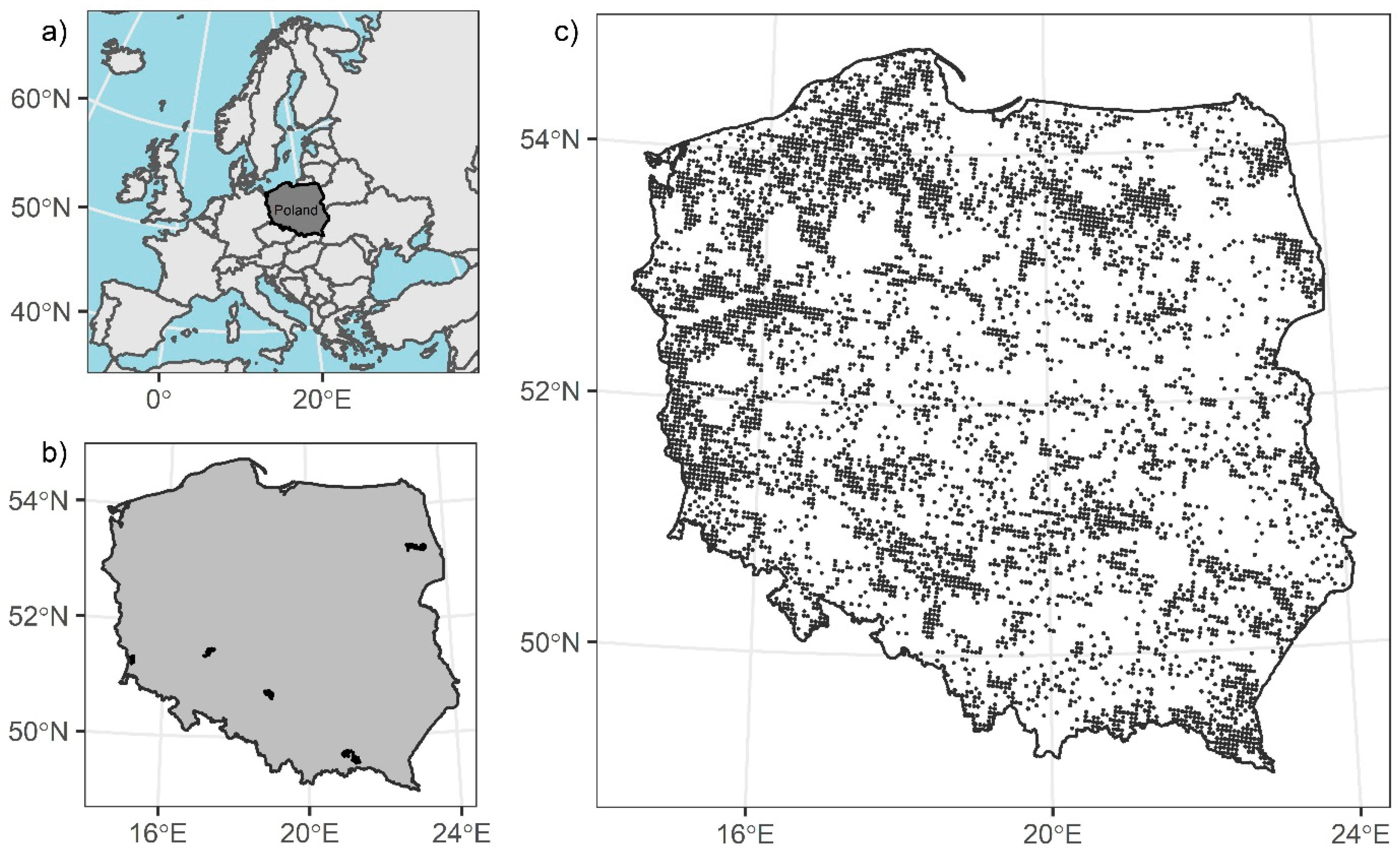
2.1. Study Area

Poland is located in Central Europe (Figure 1a) and covers a total area of 312,679 km2. According to the Central Statistical Office [20], forest covers 29.6% of the country’s area, which corresponds to 92,420 km2. Poor and moderately rich forest habitats predominate and cover 57% of the forested area which is reflected in the dominance of coniferous tree species, which dominate over 68% of the area of Polish forests [21]. According to the National Forest Inventory [22], Scots pine (Pinus sylvestris L.) is predominant in most Polish tree stands. Among the deciduous species, oaks (Quercus spp.), silver birch (Betula pendula Roth.) and black alder (Alnus glutinosa Gaertn) are the species with the largest share. In mountainous areas, the share of Norway spruce (Picea abies Karst.), silver fir (Abies alba Milland) and European beech (Fagus sylvatica L.) is more significant. Forest ownership also has an impact on its management. In Poland, public forests are predominant (80.7%), with most of them under the administration of the State Forests. The age structure is mainly represented by III and IV age classes (41–60 and 61–80 years old, respectively). As reported by the National Forest Inventory at the end of 2016, the timber resources in Polish forests reached 2587 million m3 of gross merchantable timber, out of which almost 80% is in the State Forests [21]. The mean growing stock volume of Polish forests is 269 m3/ha, which is much higher than the average in European forests (163 m3/ha) [23].

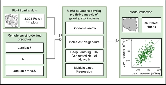
2.2. Polish National Forest Inventory Data
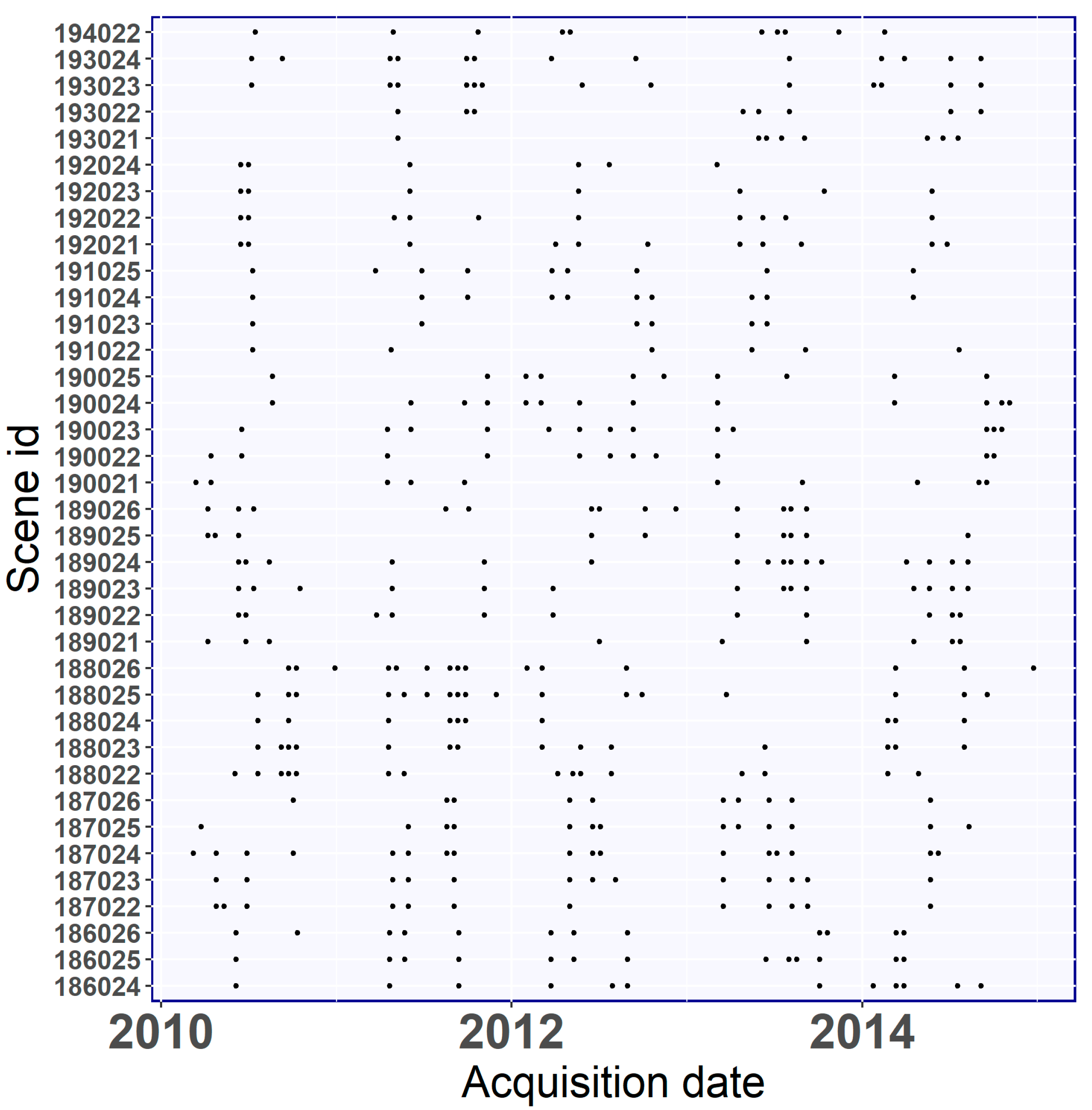
The National Forest Inventory started in Poland in 2005. This system uses a systematic scheme within a 4 km square grid of permanent sample plots. The 4 km grid is based on the pan-European 16 × 16 km forest monitoring network of the International Co-operative Programme on the Assessment and Monitoring of Air Pollution Effects on Forests [24]. Measurements of the NFI plots are performed in a 5-year inventory cycle measuring approximately 20% of the plots each year. In the first two cycles of the NFI, the sample plots were circular with 7.98 m (200 m2), 11.28 m (400 m2) and 12.62 m (500 m2) radii depending on the forest stand age. In the last recent cycle (2015–2019), a radius of 11.28 m (400 m2) was used for all plots. At each NFI sample plot, many tree and stand characteristics were measured. The diameter at breast height (DBH) was measured for all trees with a DBH ≥ 7 cm. The heights of the selected trees were measured to estimate the height curve. To obtain the GSV for a sample plot, first, the allometric models are used to predict individual tree volumes. Then, after aggregation from single trees, the plot-level GSV is calculated [25,26]. In this research, measurements from the second cycle of the NFI (2010–2014) were used since these measurements guaranteed the smallest difference between the time of the field measurements and the time of the ALS point cloud acquisition. For the analysis, 13,323 NFI sample plots were used, where the full area of the sample plot was located within the borders of a single forest stand and for which the ALS point clouds were available. The basic characteristics of the GSV at the plot level are presented in Table 1. The species share at the plot level was calculated using the volume of single trees.

2.3. Landsat Images

After considering the possibility of using other forms of optical satellite imagery, we chose the imagery of Landsat 7 ETM+ to cover the study area because the scenes are freely available at a moderate resolution (30 × 30 m) compared to other types of satellite data that require a fee (e.g., Quickbirds and Ikonos) or are not available for the years of interest (e.g., Sentinel-2). In total, Poland is covered by 37 Landsat scenes (Figure 2), so we used the Google Earth Engine Platform (GEE) to obtain a cloud-free composite image. GEE provides a full repository of Landsat data and offers the possibility to select and process images with a specific threshold of cloud cover and a specific time range, as well as quickly obtain free cloud composite images that are produced combining different images of the same scenes [27]. Based on the cloud cover thresholds (i.e., less than 10%), the solar zenith angle (i.e., less than 76°) and the specific acquisition period (i.e., 1 January 2010−31 December 2014), we found that 420 images were available for all of Poland’s area, with an average of 11 images for each Landsat scene (Figure 2). Among the 420 images selected, 24 were acquired between November and February.
For all the selected images, we used the bottom of the atmosphere reflectance values (BOA) calculated using the LEDAPS (Landsat ecosystem disturbance adaptive processing system) algorithm [28]. The images were subsequently masked for clouds using the Fmask (Function of the mask) algorithm [29]. Based on the processed images for reflectance and cloud masking, using GEE, we produced a cloud-free composite image for the whole of Poland. The spectral value of each pixel of the composite image was calculated as the ‘median’ of all Landsat images available for the specific pixel. More details on GEE and composite images can be found in Gorelick et al. [27].

2.4. Airborne Laser Scanning Point Clouds

The primary dataset for developing the GSV models in this research consisted of ALS point clouds acquired during the country-wide projects aimed mainly at creating a detail Digital Terrain Model for the whole of Poland. In the years 2011–2015, the Main Office of Geodesy and Cartography in Poland commissioned the development of altitude data using ALS technology for an area encompassing 92% of the country—i.e., 288,806 km2 of Poland. In the following years (2015–2017), data collection for other areas of the country continued. ALS data were obtained in two standards: Standard I (mainly forest and rural areas outside cities), where the point density is at least four pulses per square meter (ppsm) and Standard II (94 cities in most without forests), with a density of at least 12 ppsm. The acquisition of ALS point clouds took place from mid-October to April, that is, in the leaf-off period, which at the transverse scan angle (allowed up to 25 degrees) guaranteed good penetration of the laser beams through the stand hood to the ground. Since the second cycle of the NFI (2010–2014) took place at nearly the same time as ALS data acquisition with the ISOK project (2011–2015), the absolute time difference between the two datasets was, in most cases (90.4%), less than three years (Table 2).
The second set of ALS data used in this study included point clouds obtained in 2015 and 2016 for the REMBIOFOR project. These data were used for validation of the developed predictive models on the validation stands. The data acquisition area included 6 forest districts where the reference forest stands were established (Figure 1b). Every single validation stand was scanned with the Riegl LiteMapper LMSQ680i laser scanning system. The scanner’s operating frequencies were in the range of 300 to 400 kHz. The aircraft was flying at around 550 m above the mean ground level altitude, maintaining 30% tile-side overlap with a 60° FOV. The above mission parameters enabled the acquisition of spatially homogeneous multi-echo point clouds with average densities in the range from 10 to 14 ppsm.

2.5. Extraction of Predictor Variables

Two different sets of predictor variables were extracted from the remote sensing data associated with each NFI plot and each stand: optical metrics from Landsat cloud-free composites and ALS normalized point cloud-derived metrics.
In particular, we extracted the median value of each band of the Landsat 7 ETM+ composite image from the pixels associated with the area of each NFI plot and each reference forest stand. Based on the normalized ALS point clouds, the sets of metrics were calculated using the lidR package for R (Table 3 [30]).

2.6. Validation Data

The 360 forest stands located in 6 forest districts across Poland with a mean area of 1.1 ha were used as validation data (Figure 1b; Table 4). Field measurements were conducted in summer and autumn 2015 (four districts) and 2016 (two districts). In each stand, only trees with a DBH of at least 7 cm were measured. Moreover, in each stand, several heights for a dominant tree species were measured (minimum 20 trees). The measured trees were distributed evenly across the DBH range and forest stand layers. Height measurements were made using a Haglof Vertex IV ultrasonic hypsometer. Then, the volume for single trees was calculated using the allometric models created for Poland [25]. To calculate the GSV, the volumes of individual trees in the stand were summed and divided by the stand area. The ALS-derived metrics listed in Table 3 were calculated for each forest stand within a 30 × 30 m raster grid corresponding to the Landsat pixel size. The predicted GSV for each stand was calculated using GEE as the weighted mean from the raster cells overlapping with the stand borders. The overlapping area was used as the weight. See the GEE documentation for more in-depth information (https://developers.google.com/earth-engine/reducers_reduce_region#pixels-in-the-region).

2.7. Predictive Methods

We evaluated four methods for predicting GSV: three nonparametric approaches—Random Forest (RF), k-Nearest Neighbours (k-NN) and deep learning neural network (DL)—and one parametric approach—the multiple linear regression (LM) model.
The training set for developing the predictive models consisted of the GSV values measured in the field at the National Forest inventory plots (n = 13,323), while the validation set consisted of 360 stands with a mean area of 1.1 ha, ranging between 0.44 ha and 3.78 ha. For both the training set and validation set, the predictor variables consist of (i) Landsat metrics and (ii) ALS metrics (Table 3).
The predictive approaches were tested using three different sets of predictor variables (i.e., Landsat; ALS; and combined Landsat and ALS metrics) to compare the performance of each predictive approach using different types of predictors. Therefore, each imputation-predictive approach was optimized three times using the three different sets of predictors. In the following paragraphs, we detail how the predictive models were parametrized.
For each set of predictors (i.e., Landsat, ALS and Landsat+ALS), we calculated the variables’ importance rankings using Random Forests and calculating the percentage increase in the mean square error (IncMSE%) by removing all variables one at a time. We calculated the IncMSE% through a 5-fold-cross-validation procedure that associates the relative standard error (MSE) to each variable.
Among the 7 Landsat predictors, the 41 ALS predictors and the 48 predictors for both Landsat and ALS, we identified the relevant and irrelevant predictors by iteratively removing the variables that were identified as less important [32]. At the end of each 5-fold cross-validation, we selected the set of predictor variables that had the lowest Mean Squared Error (MSE). Therefore, we selected a set of predictor variables for Landsat, a set of predictor variables for ALS and a set of predictor variables combining the Landsat and ALS variables. Then, the three sets of predictors were used to optimize the four predictive approaches.
Each predictive approach (i.e., Random Forest, k-NN, Neural Network and Multiple Linear Regression) was optimized three times using the three sets of predictor variables selected with the procedure described above. In this section, we will describe the different predictive approaches used.

2.7.1. Random Forests

RF is a decision tree algorithm introduced by Breiman [33]. It is commonly used for the spatial prediction of forest variables using remotely sensed data [34,35,36,37,38]. RF grows a set of regression trees (ntree) with a certain depth (tdepth), using a randomly chosen subset of predictors for each one (mtry). To build trees, the out-of-bag samples (OOB) procedure is applied, where each tree is built independently based on bootstrap samples from the training dataset, while the remaining one-third of the samples are randomly left out. More details on the RF method can be found in the review of Belgiu and Drăgu [39] and in the article of Li et al. [32].
The hyperparameter optimization was performed using a random search tuning approach, through which we tested 50 randomly extracted combinations of ntree, mtry and tdepth (Table 5), searching for the combination that minimizes the Root Mean Square Error:
RMSE =   i = 1 n ( y i y ^ i ) 2 n   ,
where y i and y ^ i denote the reference and predicted values, respectively, for the i-th sample plot and n is the number of plots.
The R M S E was evaluated using k-fold cross-validation. For each hyperparameter combination, we randomly divided the NFI plots into 5 reference set units and each one was deleted in sequence and predicted using the remaining plots. Thus, each sample plot was never used for both training and testing.

2.7.2. k-Nearest Neighbours

The k-NN imputation approach is well known method often used for developing predictive models in context of applications of remote sensing data in forestry [40]. With the k-Nearest Neighbours (k-NN) technique, predictions are calculated as linear combinations of observations for sample units that are the nearest to the population units for which the predictions are desired with respect to a selected distance metric in the space of the feature (auxiliary) variables. The optimization of k-NN parameters was performed using the same procedure used for RF but optimizing k (the number of nearest neighbours), the Minkowski distance parameter (among Euclidean or Manhattan distance) and the distance metric. A full list of the tested hyperparameters is provided in Table 5.

2.7.3. Deep Learning Fully Connected Neural Network

The Deep Learning model (DL) consists of N stacked layers composed of M nodes that facilitate learning through successive representations of the input data [41]. The DL model that we used was a Fully Connected Neural Network (FCNN), in which all nodes or neurons, in one layer are connected to the nodes in the next layer. The data are transformed in each layer using weights, which are specific parameters that link the nodes of subsequent layers [42]. During training, the optimum value of the weight of each node was optimized based on the loss function, which measures the difference between the observed and predicted values. In this study, modelling was done using the TensorFlow backend.
DL models require several hyperparameters to be set: (i) the number of hidden layers, (ii) the number of nodes, (iii) the optimizer and relative Learning Rate, (iv) the number of dropout layers, (v) the percentage of dropped out units in each layer, (vi) the different activation function configurations, (vii) the different values of lambda for L1 and L2 regularization strategies, (viii) the number of epochs and (ix) the activation function.
These hyperparameters are too numerous to use the same automatic random search optimization procedure used for k-NN and RF. Therefore, we used a trial-and-error approach, which, compared to random search, is more time consuming and requires more in-depth knowledge of the model and the effects of the hyperparameters.
As for RF and k-NN, we chose the best model configuration by minimizing the RMSE resulting from the 5-fold-cross validation procedure.

2.7.4. Multiple Linear Regression

Multiple linear regression (LM) method can be defined in the form of
y i = β 0 + β 1 · x 1 i + · · · + β p · x p i + ε i ,
where i indexes the sample units, y i represents the single response variable, p ≥ 1 denotes the number of explanatory variables, j = {1, …, p} indexes the explanatory variables, β j is the respective regression coefficient and ε i denotes a random residual term with the distribution of N ( 0 , σ i 2 ) . LM does not have hyperparameters and does not require an optimization phase. However, we calculated the performance of LM with the same 5-fold-cross validation procedure used for RF, k-NN and DL.

2.8. Models Training and Validation

As a result of the previous processes, we identified the model configurations that ensure the best performance in terms of the RMSE. Then, we ultimately trained the k-NN, RF, DL and LM models with the identified configuration using all 13,323 NFI plots. We tested the best twelve models (i.e., the four predictive approaches using the three different sets of predictors) using a bootstrapping approach based on the reference stands (n = 360) to evaluate the performance using an independent dataset (never-seen-before data).
Resampling methods such as the bootstrap resampling technique can be applied to assess uncertainty for predictive approaches such as parametric and nonparametric approaches [43,44]. Bootstrapping is based on the notion of a bootstrap sample and the bootstrapping pair approach was used to construct bootstrap samples for this study [45]. We created 100,000 bootstrap samples (nboot = 100,000) that were considered to be consistent [43,45]. Each sample consisted of a sample drawn with a replacement from the original reference set with the same dimension of the original stand dataset (n = 360).
Based on each 100,000 bootstrap sample, we applied the models and calculated the RMSE as done in the optimization phase (Equation (1)). In this case, the n value was equal to the number of stands (n = 360). Moreover, we calculated the relative RMSE% as the percentage of the average ground reference value of the bootstrap samples.
For each model, at the end of the bootstrapping procedure, we calculated the mean RMSE (μ) and the RMSE% (μ%) as the mean of the RMSE. The mean of the RMSE% achieved for each bootstrap sample was calculated as
μ =   i = 1 n RMSE i b
μ % =   i = 1 n RMSE % i b ,
where RMSE i and R M S E % i are the results achieved for the i-th bootstrap sample and b is the number of bootstrap samples; in our case, b = 100,000. Using the same procedure, we calculated the R2, the bias and the relative bias for the bootstrap samples.
Moreover, we calculated confidence intervals of 95% for each parameter of performance as
μ ± t 1 α / 2   σ ( μ )
μ % ± t 1 α / 2   σ ( μ % ) ,
where α is the significant value, t 1 α / 2 is the 1 α 2 percentile of Student’s t-distribution (in our case 1.96) and σ is the standard deviation.
Additionally, the R 2 ,   RMSE %   and   bias % were calculated and analysed for the dominant tree species with at least 20 validation stands available.

3. Results

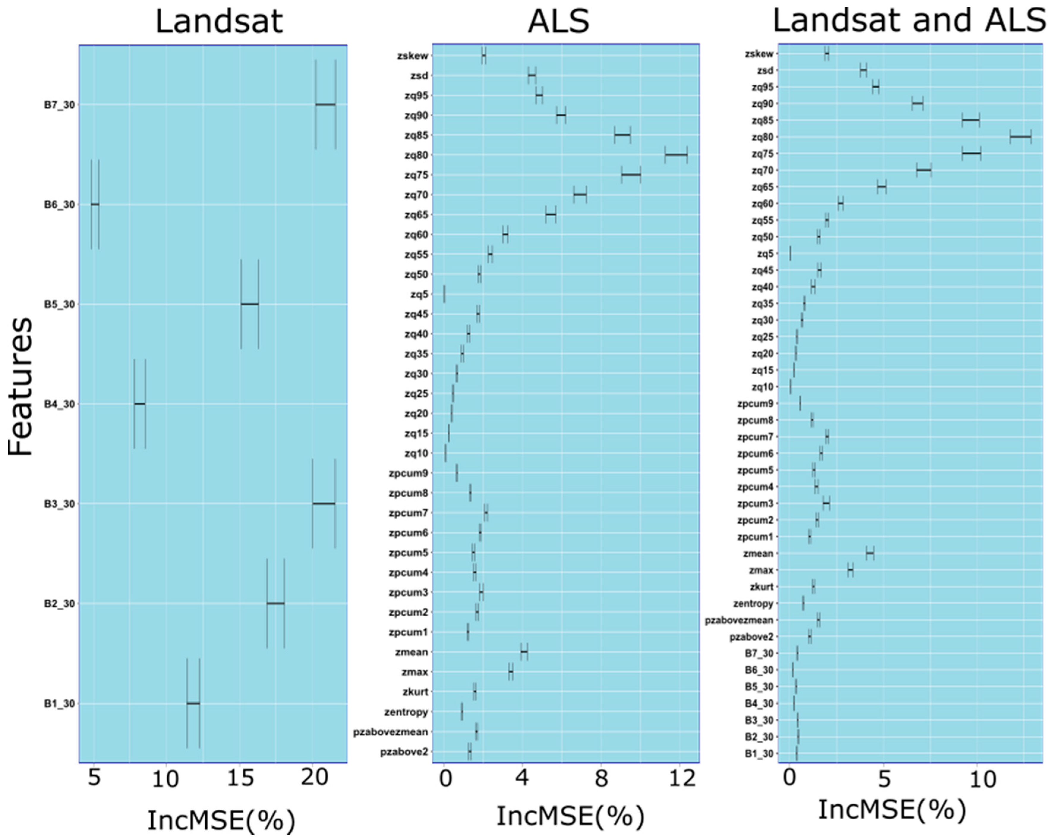
3.1. Set of Predictor Variables

Importance ranking using Random Forests and calculation of the percentage increase in the mean square error (IncMSE%) by removing all variables one at a time identified the best sets of predictor variables for the three sets of predictors (i.e., Landsat, ALS and Landsat+ALS).
The sets of predictor variables for the Landsat predictors consisted of all the bands (except for Band 6) being removed (Figure 3). However, for the ALS predictors, we removed zq10 and zq5 (Figure 3). For the set of a predictor that combined Landsat and ALS, we found that the same variables removed from the other two sets were also excluded (i.e., B6, zq10 and zq5; Figure 3).

3.2. Optimization Results

Each predictive approach was optimized using the three sets of predictors to search for the hyperparameters that can achieve the lowest RMSE. The results of the calibration of the RF and KNN models are reported in Table 6. Using the 5-fold-cross validation procedure, we found that under the same approach, the configurations of the hyperparameters (Table 6) remain similar if different sets of predictors are used.
In case of the neural network configurations for the DL models we matched the number of nodes in the input layer with the number of predictors. The number of hidden layers was two with 70 nodes each and LeakyReLU activation functions [46]. Moreover, the number of dropout layers was two, with the percentage of nodes randomly dropped out equal to 30%. The L1 and L2 regularization layers were not necessary and the selected optimizer was rmsprop [47].

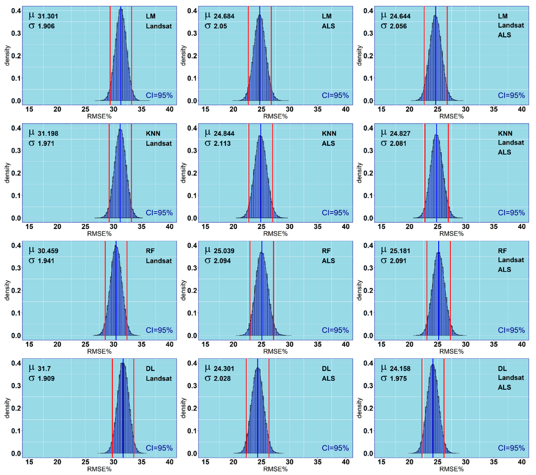
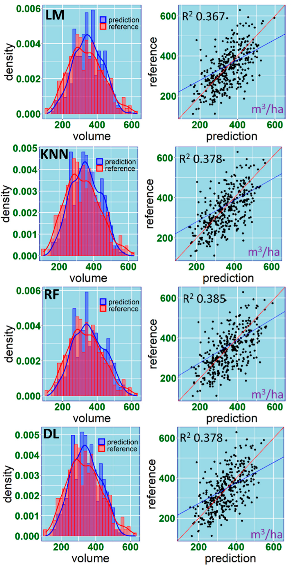
3.3. Performance Assessment

The results of the bootstrapping procedure were comparable among different predictive approaches with the same sets of predictors. As shown in Figure 4, the results are consistent and comparable in terms of the confidence interval and distribution of the errors. Using the Landsat predictors, we found that all predictive approaches achieved results for an RMSE between 102.10 and 106.24 m3/ha and an RMSE% between 30.45% and 31.69% with the RF that achieved the highest accuracy (Table 7). Using the ALS predictors, we found that all the predictive methods achieved RMSE results between 81.43 and 83.90 m3/ha and RMSE% results between 24.30% and 25.03% with the DL that achieved the highest accuracy. Using the Landsat and ALS predictors, the evaluated predictive approaches achieved results for an RMSE between 80.98 and 84.41 m3/ha and an RMSE% between 24.16% and 25.18% with the RF that achieved the lowest accuracy and the DL the highest accuracy.
All predictive approaches have similar results for R2 (Figure 5). Using Landsat, only the R2 dropped to 0.01. Similarly, using only Landsat, the bias was large, ranging between 40.39 and 36.56 m3/ha. On the other hand, Landsat made an important contribution to DL when used together with the ALS. Indeed, when using DL with just the ALS, the bias was −11.64 m3/ha but while using both the Landsat and the ALS, the bias dropped to −7.31 m3/ha.

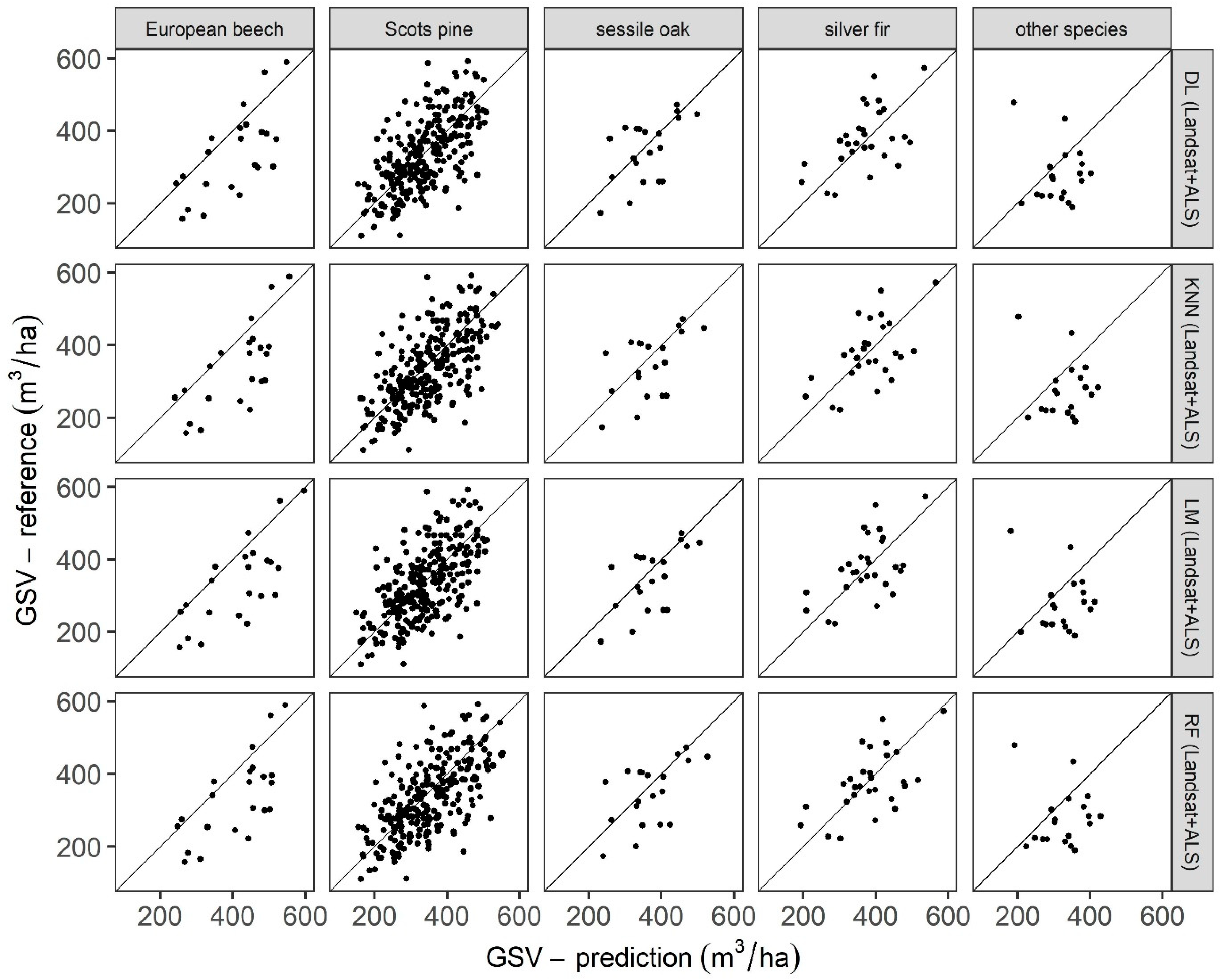
3.4. Performance Assessment per Dominant Tree Species

From the set of 360 validation stands, there were four dominant tree species for which at least 20 stands were available: European beech, Scots pine, sessile oak and silver fir. The other species were joined to one group of 19 stands. For these groups of stands, the performance of the models developed based on Landsat- and ALS-derived predictors was analysed (Figure 6, Table 8). The RMSE was relatively low for oak, pine and fir regardless of the predictive method, varying from 72.61 m3/ha (20.99%) for oak-dominated stands with the DL method to 80.00 m3/ha (24.06%) for pine-dominated stands predicted with the RF model. A considerably larger RMSE was obtained for the beech-dominated stand varying from 106.94 m3/ha (DL) to 110.19 m3/ha (LM). For beech-dominated stands, large systematic errors (bias) were also observed for all evaluated predictive methods: from −20.19% (−66.62 m3/ha) for the DL model up to −23.71% (−78.55 m3/ha) for LM. The relative bias for pine, oak and fir varied from 0.70% (fir; RF) to −6.73% (oak, LM). The R2 averaged through all predictive methods was the highest for beech-dominated stands (0.50) and the lowest for fir-dominated stands (0.30). The R2 was also low for the group of 19 stands dominated by “other species” (0.13).

4. Discussion

In this article, four predictive approaches (LM, KNN, RF and DL) trained based on NFI plots combined with ALS point clouds and Landsat images were evaluated for predicting GSV at the stand level. Three sets of predictor variables were tested (ALS, Landsat and Landsat+ALS) for all methods. Validation of the developed models was performed on 360 forest stands measured in the field.
When creating the Landsat mosaic, we did not divide the Landsat images into leaf-on (396 images) and leaf-off (24 images) datasets. Although we are aware that mixing leaf-on and leaf-off images is not a perfect approach, we assumed that since the final reflectance value was calculated as the median, the rare leaf-off images would not affect the final image consistently. On the other hand, rare high quality leaf-off images (cloud cover < 10% and solar zenith angle smaller than 76°) selected in winter can be informative for evergreen trees and areas when there are no images acquired during the leaf-on season, which may occur when algorithms are applied over huge areas.
The obtained results showed that there are no considerable differences in accuracy between the evaluated predictive approaches (Table 7, Figure 4 and Figure 5). Generally, the DL method provided the lowest RMSE and bias; however, the differences between models were minimal. Larger differences between the predictive models were observed when validating within groups of dominant tree species. The results show that multiple linear regression (LM) can provide satisfactory results but there are no or only small, benefits from using more advanced methods, including machine learning (KNN and RF) or deep learning (DL). The linear model was used by Nilsson et al. [17] for country-level forest variables estimation in Sweden. The RMSE of 24.69% obtained in our study (LM) regardless of tress species is larger than that obtained by Nilsson et al. ([17]; RMSE: 17.2%–22.0%); however, this might be related to the higher species and structural variability of Polish forests. Parametric and nonparametric methods each have their own pros and cons. Previous works [9,48] pointed to the undoubted advantage of classic multiple linear regression, highlighting the ease of interpreting the model. The advantage of LM is also its ability to extrapolate extreme values. The construction of such models, however, requires more experience and more work for the selection of appropriate predictors. This problem disappears with the nonparametric methods of KNN, RF and DL used in this paper. These models can also provide good performance in the case of non-linear relationships between variables. However, the possibility of more frequent model overfitting and poor results in the case of overly small observation sets are potential disadvantages of these approaches [49,50].
The obtained results showed differences in the performance of the developed predictive models between dominant tree species. Nilsson et al. [17] reported for Sweden that when the proportion of broadleaved trees increased to 76%, the RMSE% of the GSV estimation increased to 27.9%. For our study, a similar relationship was observed. The model performance was relatively good for pine and fir, moderate for oak and the worst for beech. However, the obtained differences in RMSE% for coniferous and broadleaved stands were not so obvious. For example, the RMSE% for oak-dominated stands was even lower than that for pine-dominated stands. We observed that the systemic error (bias) is higher for stands dominated by broadleaved trees. In the case of beech-dominated stands, the relative bias increased to more than −20%, meaning that the developed models are not appropriate for these kinds of stands. It can be expected that creating species-specific models will improve the accuracy and reduce model bias [19]. However, the large overestimation of GSV for broadleaved stands is likely the result of using the ALS point clouds of different characteristics for model validation, and for model development. In cases when the ALS point clouds are collected with different pulse densities and at different times throughout the year, the ALS metrics obtained for broadleaved trees might not be comparable between two acquisitions. Our results suggest that such an approach can be acceptable for the prediction of GSV in coniferous forests but not in areas dominated by broadleaved species. To deal with this issue, predictive models for broadleaved trees could be developed based on metrics derived from the Canopy Height Model instead of using the point cloud-derived metrics.
In our research, we tested a deep learning method as a fully connected neural network using the same predictor variables applied in the other three predictive methods. When validating the results regardless of the dominant tree species, the best model accuracy among all tested predictive approaches and sets of predictor variables was obtained with the DL utilizing Landsat+ALS variables (RMSE% = 24.2; bias% = −2.2%) but this performance was only slightly better than that of the other tested methods. However, to derive reliable conclusions about the performance of DL for GSV predictions, different neural network architecture types must be evaluated, including the Convolutional Neural Network (CNN). Deep learning with CNN architecture—especially 3D CNN—can interpret raw data (e.g., ALS point clouds) without the need for human-derived explanatory variables such as height percentiles or density metrics, which are usually used as predictor variables in other imputation-predictive methods [51,52]. Ayrey et al. [51] showed that 3D CNN can considerably outperform the random forest method in predicting forest parameters based on ALS and satellite data.
In similar studies on using NFI plots and ALS point clouds for GSV estimation [17,18,19], the detailed selection of training plots and high accuracy measurements of the plot centres were used, while in our study, accurate coordinates of the plot centres were not available. This is likely the main reason for the relatively low R2 values that we obtained. Nevertheless, our study shows that for coniferous species (Scots pine and silver fir), relatively low RMSE% (22%–23%) and bias% (1%) can be obtained for stand-level GSV predictions when combining ALS point clouds and Landsat images with NFI data, even when the positional errors of the field plots vary from several to about 15 m. It can be assumed that collecting accurate information about the plot centre coordinates in the next cycles of the Polish NFI may increase the accuracy of the predictive models of GSV. However, McRoberts et al. [53] observed only a small decrease in the standard error of the mean aboveground biomass in ALS-assisted estimates of aboveground biomass when using survey-grade GPS receivers with sub-meter accuracy compared to field grade GPS receivers with a 5–10 m accuracy. The aforementioned authors concluded that the high costs of acquiring a survey-grade GPS receiver are not justified in the case of ALS-assisted estimates of aboveground biomass at the national scale level in the USA.
Notably, in our study, for some of the NFI plots, there was up to a 5-year difference between the year of laser scanning and the year of the field survey. This difference may provide additional noise in the data used for training the predictive models because of tree growth, thinning activities, clear cutting or the occurrence of forest disturbances. As we are aware of these limitations, we assumed that the influence of these imperfections (positional inaccuracy and time lag) in the NFI data might be mitigated by using many training plots (13,323) through averaging the model parameters. We also maintain that a few-year difference between field measurements on NFI plots and the available ALS point clouds (or image-derived point clouds) may often be the case in real-world applications. Thus, we decided to use all NFI plots for which ALS data were available. The influence of time lag on the accuracy of GSV predictive models should be analysed in future studies.
When considering the forest management inventory at a local scale, an absolute bias of about 0%–3% (like that obtained for coniferous tree species) can be acceptable. However, this level of systematic error might be problematic for large areas of ALS-assisted estimates with GSV. The obtained bias might partially be the result of the abovementioned inaccuracies in the NFI data but it might also be the result of resolution difference between the differently sized training field plots (200 m2, 400 m2 and 500 m2) and grids used for the model predictions (30 × 30 m; 900 m2). Nevertheless, we decided to use a 30 × 30 m resolution grid for prediction to avoid resampling and average the Landsat-derived predictors. Packalen et al. [54] reported that a resolution mismatch between the field plot size and grid cell size used for predictions caused only a small increase of bias in ABA. The authors indicated that a higher prediction resolution compared to training resolution caused an underestimation of AGB. However, in our study, overestimation of GSV was observed in most cases, even though the prediction grid was larger than the training sample size.
Future research should evaluate how the time lag between NFI and ALS data influences the predictions of growing stock volume at the national level. It would also be valuable to evaluate more complex DL models based on raw ALS point cloud data including convolutional layers. On the other hand, simpler multiple regression models based on Canopy Height Models may be potentially more transferable compared to point cloud-based models, especially for stands dominated by broadleaved trees. The use of predictors from Sentinel-2 + ALS instead of Landsat+ALS also seems worth exploring.

5. Conclusions

Several conclusions were drawn from this study. First, using Landsat-derived predictors together with ALS only slightly increased the accuracy of GSV predictions compared to using only ALS-derived predictors. Second, the deep learning method in the form of fully connected layers does not provide considerably more accurate predictions of GSV compared to the LM, KNN and RF approaches. To benefit more from the deep learning approach, larger datasets and network architectures including convolutional layers are likely needed. Third, NFI plots with positional errors in the order of several to about 15 m combined with ALS point clouds can be used for the development of relatively accurate predictive models of the growing stock volume. In cases when a relatively large number of NFI plots is available for model training, the influence of positional inaccuracies and the time lag of NFI plots is likely mitigated partially by averaging the model parameters. The demonstrated approach is applicable for coniferous stands even when the ALS point clouds of different pulse densities are used for model training and prediction. However, when applied to forest stands dominated by broadleaved trees, large systematic errors may occur. Further research aimed at improving the integration methods of NFI data with remote sensing data is desirable, especially in the context of model transferability in broadleaved forests. Integrating NFI with remotely sensed data could provide substantial cost savings in the forest management inventory at a local scale.

Author Contributions

Conceptualization, P.H., G.C. and J.S.; methodology, P.H., G.C., S.F. and F.G.; formal analysis, P.H., S.F. and F.G.; data curation, P.H., J.S., K.S., K.P., G.K., K.M., M.L., M.C. and P.W.; writing—original draft preparation, P.H., S.F., G.C., F.G. and J.S.; writing—review and editing, K.S., K.P., G.K., K.M., M.L., M.C. and P.W.; funding acquisition, J.S. and K.S. All authors have read and agreed to the published version of the manuscript.

Funding

This research was supported by the projects REMBIOFOR and I-MAESTRO. The project “REMBIOFOR” was financed by The National Centre for Research and Development in Poland under the programme BIOSTRATEG, agreement no. BIOSTRATEG1/267755/4/NCBR/2015. The Project Innovative forest MAnagEment STrategies for a Resilient biOeconomy under climate change and disturbances (I-MAESTRO) is supported under the umbrella of ForestValue ERA-NET co-funded by the National Science Centre, Poland and the French Ministry of Agriculture, Agrifood and Forestry, as well as the French Ministry of Higher Education, Research and Innovation, German Federal Ministry of Food and Agriculture (BMEL) via the Agency for Renewable Resources (FNR), the Slovenian Ministry of Education, Science and Sport (MIZS). ForestValue received funding from the European Union’s Horizon 2020 research and innovation programme under grant agreement N° 773324.

Conflicts of Interest

The authors declare no conflict of interest.

References

  1. Kangas, A.; Astrup, R.; Breidenbach, J.; Fridman, J.; Gobakken, T.; Korhonen, K.T.; Maltamo, M.; Nilsson, M.; Nord-Larsen, T.; Næsset, E.; et al. Remote sensing and forest inventories in Nordic countries—Roadmap for the future. Scand. J. For. Res. 2018, 7581, 1–16. [Google Scholar] [CrossRef] [Green Version]
  2. Tomppo, E.; Gschwantner, T.; Lawrence, M.; McRoberts, R.E. National Forest Inventories: Pathways for Common Reporting; Springer: Dordrecht, The Netherlands, 2010; ISBN 9789048132324. [Google Scholar]
  3. Gschwantner, T.; Lanz, A.; Vidal, C.; Bosela, M.; Di Cosmo, L.; Fridman, J.; Gasparini, P.; Kuliešis, A.; Tomter, S.; Schadauer, K. Comparison of methods used in European National Forest Inventories for the estimation of volume increment: Towards harmonisation. Ann. For. Sci. 2016. [Google Scholar] [CrossRef] [Green Version]
  4. Næsset, E. Area-Based Inventory in Norway—From Innovation to an Operational Reality. In Forestry Applications of Airborne Laser Scanning: Concepts and Case Studies; Springer: Dordrecht, The Netherlands, 2014; pp. 215–240. [Google Scholar]
  5. White, J.C.; Coops, N.C.; Wulder, M.A.; Vastaranta, M.; Hilker, T.; Tompalski, P. Remote Sensing Technologies for Enhancing Forest Inventories: A Review. Can. J. Remote Sens. 2016, 42, 619–641. [Google Scholar] [CrossRef] [Green Version]
  6. Wulder, M.A.; Bater, C.W.; Coops, N.C.; Hilker, T.; White, J.C. The role of LiDAR in sustainable forest management. For. Chron. 2008, 84, 807–826. [Google Scholar] [CrossRef] [Green Version]
  7. Socha, J.; Hawryło, P.; Pierzchalski, M.; Stereńczak, K.; Krok, G.; Wężyk, P.; Tymińska-Czabańska, L. An allometric area-based approach—A cost-effective method for stand volume estimation based on ALS and NFI data. For. Int. J. For. Res. 2019, 93, 344–358. [Google Scholar] [CrossRef]
  8. Kurz, W.A.; Dymond, C.C.; White, T.M.; Stinson, G.; Shaw, C.H.; Rampley, G.J.; Smyth, C.; Simpson, B.N.; Neilson, E.T.; Trofymow, J.A.; et al. CBM-CFS3: A model of carbon-dynamics in forestry and land-use change implementing IPCC standards. Ecol. Model. 2009, 220, 480–504. [Google Scholar] [CrossRef]
  9. White, J.C.; Wulder, M.A.; Varhola, A.; Vastaranta, M.; Coops, N.C.; Cook, B.D.; Pitt, D.G.; Woods, M. A Best Practices Guide for Generating Forest Inventory Attributes from Airborne Laser Scanning Data Using an Area-Based Approach; Technical Report FI-X-010; The Canadian Wood Fibre Centre: Victoria, BC, Canada, 2013. [Google Scholar]
  10. Næsset, E. Estimating timber volume of forest stands using airborne laser scanner data. Remote Sens. Environ. 1997, 61, 246–253. [Google Scholar] [CrossRef]
  11. Brach, M.; Stereńczak, K.; Bolibok, L.; Kwaśny, Ł.; Krok, G.; Laszkowski, M. Impacts of forest spatial structure on variation of the multipath phenomenon of navigation satellite signals. Folia For. Pol. 2019, 61, 3–21. [Google Scholar] [CrossRef] [Green Version]
  12. Stereńczak, K.; Lisańczuk, M.; Parkitna, K.; Mitelsztedt, K.; Mroczek, P.; Miścicki, S. The influence of number and size of sample plots on modelling growing stock volume based on airborne laser scanning. Drewno 2018, 61. [Google Scholar] [CrossRef]
  13. Gobakken, T.; Næsset, E. Assessing effects of positioning errors and sample plot size on biophysical stand properties derived from airborne laser scanner data. Can. J. For. Res. 2009, 39, 1036–1052. [Google Scholar] [CrossRef]
  14. Mauro, F.; Valbuena, R.; Manzanera, J.A.; García-Abril, A. Influence of global navigation satellite system errors in positioning inventory plots for treeheight distribution studies. Can. J. For. Res. 2011, 41, 11–23. [Google Scholar] [CrossRef]
  15. Tomppo, E. Satellite image-based National Forest Inventory of Finland. In Proceedings of the ISPRS, COMISSION VII, Mid-Term Symposium Global and Environmental Monitoring, Techniques and Impacts, Victoria, BC, Canada, 17–21 September 1990; pp. 419–424. [Google Scholar]
  16. Chirici, G.; Giannetti, F.; McRoberts, R.E.; Travaglini, D.; Pecchi, M.; Maselli, F.; Chiesi, M.; Corona, P. Wall-to-wall spatial prediction of growing stock volume based on Italian National Forest Inventory plots and remotely sensed data. Int. J. Appl. Earth Obs. Geoinf. 2020, 84, 101959. [Google Scholar] [CrossRef]
  17. Nilsson, M.; Nordkvist, K.; Jonzén, J.; Lindgren, N.; Axensten, P.; Wallerman, J.; Egberth, M.; Larsson, S.; Nilsson, L.; Eriksson, J.; et al. A nationwide forest attribute map of Sweden predicted using airborne laser scanning data and field data from the National Forest Inventory. Remote Sens. Environ. 2017, 194, 447–454. [Google Scholar] [CrossRef]
  18. Hollaus, M.; Dorigo, W.; Wagner, W.; Schadauer, K.; Höfle, B.; Maier, B. Operational wide-area stem volume estimation based on airborne laser scanning and national forest inventory data. Int. J. Remote Sens. 2009, 30, 5159–5175. [Google Scholar] [CrossRef]
  19. Nord-Larsen, T.; Schumacher, J. Estimation of forest resources from a country wide laser scanning survey and national forest inventory data. Remote Sens. Environ. 2012, 119, 148–157. [Google Scholar] [CrossRef]
  20. CSO. Statistical Yearbook of Forestry; Statistics Poland: Warsaw, Poland, 2019. (In Polish)
  21. SFIC. Forests in Poland; The State Forests Information Centre: Warsaw, Poland, 2018. [Google Scholar]
  22. NFI National Forest Inventory. Wielkoobszarowa Inwentaryzacja Stanu Lasów, Wyniki za Okres 2014–2018; Biuro Urządzania Lasu i Geodezji Leśnej: Warsaw, Poland, 2018. (In Polish) [Google Scholar]
  23. Forest Europe. State of Europe’s Forests. In Proceedings of the Ministerial Conference on the Protection of Forests in Europe, Madrid, Spain, 20–21 October 2015. [Google Scholar]
  24. ICP ICP Forests Manual. Manual on Methods and Criteria for Harmonized Sampling, Assessment, Monitoring and Analysis of the Effects of Air Pollution on Forests; Thünen Institute Forest Ecosystems: Eberswalde, Germany, 2016. [Google Scholar]
  25. Bruchwald, A.; Rymer-Dudzińska, T.; Dudek, A.; Michalak, K.; Wróblewski, L.; Zasada, M. Wzory empiryczne do określania wysokości i pierśnicowej liczby kształtu grubizny drzewa. Sylwan 2000, 144, 5–12. [Google Scholar]
  26. Gschwantner, T.; Alberdi, I.; Balázs, A.; Bauwens, S.; Bender, S.; Borota, D.; Bosela, M.; Bouriaud, O.; Cañellas, I.; Donis, J.; et al. Harmonisation of stem volume estimates in European National Forest Inventories. Ann. For. Sci. 2019, 76. [Google Scholar] [CrossRef] [Green Version]
  27. Gorelick, N.; Hancher, M.; Dixon, M.; Ilyushchenko, S.; Thau, D.; Moore, R. Google Earth Engine: Planetary-scale geospatial analysis for everyone. Remote Sens. Environ. 2017, 202, 18–27. [Google Scholar] [CrossRef]
  28. Schmidt, G.; Jenkerson, C.B.; Masek, J.; Vermote, E.; Gao, F. Landsat Ecosystem Disturbance Adaptive Processing System (LEDAPS) Algorithm Description; U.S. Geological Survey: Reston, VA, USA, 2013.
  29. Zhu, Z.; Woodcock, C.E. Object-based cloud and cloud shadow detection in Landsat imagery. Remote Sens. Environ. 2012, 118, 83–94. [Google Scholar] [CrossRef]
  30. Roussel, J.-R.; Auty, D. lidR: Airborne LiDAR Data Manipulation and Visualization for Forestry Applications. R Package Version 2.2.2. Available online: https://CRAN.R-project.org/package=lidR2020 (accessed on 28 January 2020).
  31. Woods, M.; Lim, K.; Treitz, P. Predicting forest stand variables from LiDAR data in the Great Lakes—St. Lawrence forest of Ontario. For. Chron. 2008, 84, 827–839. [Google Scholar] [CrossRef] [Green Version]
  32. Li, I.Z.W.; Xin, X.P.; Huan, T.A.N.G.; Fan, Y.A.N.G.; Chen, B.R.; Zhang, B.H. Estimating grassland LAI using the Random Forests approach and Landsat imagery in the meadow steppe of Hulunber, China. J. Integr. Agric. 2017, 16, 286–297. [Google Scholar] [CrossRef]
  33. Breiman, L. Random Forests. Mach. Learn. 2001, 45, 5–32. [Google Scholar] [CrossRef] [Green Version]
  34. Baccini, A.; Goetz, S.J.; Walker, W.S.; Laporte, N.T.; Sun, M.; Sulla-Menashe, D.; Hackler, J.; Beck, P.S.A.; Dubayah, R.; Friedl, M.A.; et al. Estimated carbon dioxide emissions from tropical deforestation improved by carbon-density maps. Nat. Clim. Chang. 2012, 2, 182–185. [Google Scholar] [CrossRef]
  35. Evans, J.S.; Cushman, S.A. Gradient modeling of conifer species using random forests. Landsc. Ecol. 2009, 24, 673–683. [Google Scholar] [CrossRef]
  36. Falkowski, M.J.; Evans, J.S.; Martinuzzi, S.; Gessler, P.E.; Hudak, A.T. Characterizing forest succession with lidar data: An evaluation for the Inland Northwest, USA. Remote Sens. Environ. 2009, 113, 946–956. [Google Scholar] [CrossRef] [Green Version]
  37. Houghton, R.A. Balancing the Global Carbon Budget. Annu. Rev. Earth Planet. Sci. 2007, 35, 313–347. [Google Scholar] [CrossRef] [Green Version]
  38. Stumpf, A.; Kerle, N. Object-oriented mapping of landslides using Random Forests. Remote Sens. Environ. 2011, 115, 2564–2577. [Google Scholar] [CrossRef]
  39. Belgiu, M.; Drăgu, L. Random forest in remote sensing: A review of applications and future directions. ISPRS J. Photogramm. Remote Sens. 2016, 114, 24–31. [Google Scholar] [CrossRef]
  40. Chirici, G.; Mura, M.; McInerney, D.; Py, N.; Tomppo, E.O.; Waser, L.T.; Travaglini, D.; McRoberts, R.E. A meta-analysis and review of the literature on the k-Nearest Neighbors technique for forestry applications that use remotely sensed data. Remote Sens. Environ. 2016, 176, 282–294. [Google Scholar] [CrossRef]
  41. Goodfellow, I.; Bengio, Y.; Courville, A. Deep Learning; MIT Press: Cambridge, MA, USA, 2016. [Google Scholar]
  42. Chollet, F. Deep Learning with Python; Manning Publications Co.: New York, NY, USA, 2018. [Google Scholar]
  43. Mura, M.; McRoberts, R.E.; Chirici, G.; Marchetti, M. Statistical inference for forest structural diversity indices using airborne laser scanning data and the k-Nearest Neighbors technique. Remote Sens. Environ. 2016, 186, 678–686. [Google Scholar] [CrossRef]
  44. McRoberts, R.E. Estimating forest attribute parameters for small areas using nearest neighbors techniques. For. Ecol. Manag. 2012, 272, 3–12. [Google Scholar] [CrossRef]
  45. Efron, B.; Tibshirani, R.J. An Introduction to the Bootstrap; Chapman & Hall/CRC: Boca Raton, FL, USA, 1994. [Google Scholar]
  46. Jebadurai, J.; Jebadurai, I.J.; Paulraj, G.J.L.; Samuel, N.E. Super-resolution of digital images using CNN with leaky ReLU. Int. J. Recent Technol. Eng. 2019, 8, 210–212. [Google Scholar] [CrossRef]
  47. Huk, M. Stochastic Optimization of Contextual Neural Networks with RMSprop BT—Intelligent Information and Database Systems; Nguyen, N.T., Jearanaitanakij, K., Selamat, A., Trawiński, B., Chittayasothorn, S., Eds.; Springer International Publishing: Cham, Switzerland, 2020; pp. 343–352. [Google Scholar]
  48. Miścicki, S.; Stereńczak, K. Określanie miąższości i zagęszczenia drzew w drzewostanach centralnej Polski na podstawie danych lotniczego skanowania laserowego w dwufazowej metodzie inwentaryzacji zasobów drzewnych. Leśne Pr. Badaw. 2013, 74, 127–136. [Google Scholar] [CrossRef] [Green Version]
  49. Guyon, I.; Elisseeff, A. An introduction to variable and feature selection. J. Mach. Learn. Res. 2003, 3, 1157–1182. [Google Scholar] [CrossRef] [Green Version]
  50. Straub, C.; Weinacker, H.; Koch, B. A comparison of different methods for forest resource estimation using information from airborne laser scanning and CIR orthophotos. Eur. J. For. Res. 2010, 129, 1069–1080. [Google Scholar] [CrossRef]
  51. Ayrey, E.; Hayes, D.J.; Kilbride, J.B.; Fraver, S.; Kershaw, J.A.; Cook, B.D.; Weiskittel, A.R. Synthesizing Disparate LiDAR and Satellite Datasets through Deep Learning to Generate Wall-to-Wall Regional Forest Inventories. BioRxiv 2019, 580514. [Google Scholar] [CrossRef]
  52. Ayrey, E.; Hayes, D.J. The use of three-dimensional convolutional neural networks to interpret LiDAR for forest inventory. Remote Sens. 2018, 10, 649. [Google Scholar] [CrossRef] [Green Version]
  53. McRoberts, R.E.; Chen, Q.; Walters, B.F.; Kaisershot, D.J. The effects of global positioning system receiver accuracy on airborne laser scanning-assisted estimates of aboveground biomass. Remote Sens. Environ. 2018, 207, 42–49. [Google Scholar] [CrossRef]
  54. Packalen, P.; Strunk, J.; Packalen, T.; Maltamo, M.; Mehtätalo, L. Resolution dependence in an area-based approach to forest inventory with airborne laser scanning. Remote Sens. Environ. 2019, 224, 192–201. [Google Scholar] [CrossRef]
Figure 1. Localization of Poland in Europe (a) with the distribution of the reference forest stands ((b); black polygons) and the distribution of NFI (National Forest Inventory) plots in Poland ((c); black dots).
Remotesensing 12 03331 g001
Figure 2. Numbers of the images available for each of the Landsat Scenes (black dots represent the available images).
Remotesensing 12 03331 g002
Figure 3. Importance ranking of Random Forests for each type of predictor: Landsat, ALS and Landsat and ALS. The graph reports the percentage increase in the mean square error (IncMSE%) of each type of predictor.
Remotesensing 12 03331 g003
Figure 4. Results of the bootstrapping procedure for each considered approach (LM—multiple linear regression, KNN—k-nearest neighbours, RF—random forests and DL—deep learning) using different sets of predictor variables (Landsat, ALS and Landsat+ALS). The red line identifies the confidence interval.
Remotesensing 12 03331 g004
Figure 5. Observed vs. predicted values of GSV (growing stock volume) for 360 validation stands for each considered predictive approach (LM—multiple linear regression, KNN—k-nearest neighbours, RF—random forests and DL—deep learning) for the best set of predictors (Landsat+ALS).
Remotesensing 12 03331 g005
Figure 6. Observed vs. predicted values of GSV (growing stock volume) for validation stands obtained with the best set of predictors (Landsat+ALS) and grouped by dominant tree species and predictive approach (DL—deep learning, KNN—k-nearest neighbours, LM—multiple linear regression and RF—random forests).
Remotesensing 12 03331 g006
Table 1. Characteristics of NFI plots used for the development of the GSV (growing stock volume) models (n = 13,323).
Dominant Tree
Species
Number of PlotsPercentage of Plots
(%)
Minimum GSV (m3/ha)Mean
GSV (m3/ha)
Maximum GSV (m3/ha)Standard Deviation of GSV (m3/ha)
Scots pine833462.60.2300.7935.1139.6
silver birch9046.80.3192.8708.4119.8
Norway spruce 7315.50.4309.31069.0200.8
European beech 7085.30.1351.81452.8220.6
sessile oak 6805.10.2296.01237.3186.0
other species6635.00.2243.41347.1174.0
common alder 5774.30.7270.9908.3165.5
silver fir4593.42.7368.01338.0217.5
European larch2672.00.3253.0795.1181.0
Table 2. Maximum absolute time difference between the time of the field measurements at the NFI plots and the time of the ALS (airborne laser scanning) point cloud acquisition.
Maximum Absolute Difference between NFI and ALS
(Years)
Number of PlotsPercentage of Plots
(%)
1520939.1
2424631.9
3258819.4
410928.2
51881.4
Table 3. Predictor variables calculated for the NFI plots and used for the development of the GSV (growing stock volume) models.
Description of Predictor VariablesAcronyms
Bottom of atmosphere reflectance of Landsat 7 ETM+ spectral bands B1_30, B2_30, B_3_30, B4_30, B5_30, B6_30, B7_30
Mean value of point heights (m)zmean
Maximum value of point heights (m)zmax
Standard deviation of point heights (m)zsd
Skewness of point heightsZskew
Kurtosis of point heightsZkurt
Percentile values of point heights: 5th, 10th, 15th, …, 95th (m)zq5, zq10, zq15, …, zq95
Entropy calculated as a normalized Shannon vertical complexity indexzentropy
Percentage of all returns above 2 m (%)pzabove2
Percentage of all returns above zmean (%)pzabovezmean
Cumulative percentage of returns from nine height layers. The height measurements were divided into 10 equal intervals according to Reference [31] (%)zpcum1, zpcum2, zcum3, …, zpcum9
Table 4. Characteristics of stands used for model validation (n = 360; mean stand area = 1.1 ha; GSV—growing stock volume).
Dominant Tree
Species
Number of StandsPercentage of Stands
(%)
Minimum GSV (m3/ha)Mean
GSV (m3/ha)
Maximum GSV (m3/ha)Standard Deviation of GSV (m3/ha)
Scots pine27075.0111.0332.6593.097.4
silver fir298.1223.0387.7629.097.4
European beech226.1158.0336.0590.0116.3
sessile oak205.6174.0348.0473.086.8
other species195.3190.0277.6479.077.7
Table 5. Set of tested parameters for each nonparametric predictive approach (KNN—k-nearest neighbours, RF—random forests and DL—deep learning).
ModelHyperparameterValuesTuning Method
KNNK1–40Random Search
Minkowski distance Euclidean distance, Manhattan distance
Distance metrics Unweighted, Weighted, Inverse, Reciprocal
RFntree100–500Random Search
mtry2—number of predictors
tdepth2–10
DLHidden layersTrial-and-error
Nodes
Optimizer
Learning Rate
Dropout layers
Dropout percentage
Activation functions
Regularization layers
L1 regularization
L2 regularization
Table 6. The best hyperparameter configurations selected for each predictive approach and each set of predictors (RF—random forest, k-NN—k-nearest neighbours).
Predictive ApproachPredictorsConfigurations
RF mtry tdepth ntree
Landsat29500
ALS26500
Landsat+ALS23500
k-NN kmaxdistancekernel
Landsat36Manhattanunweighted
ALS37Manhattaninverse
Landsat+ALS35Manhattan inverse
Table 7. Performance of the developed growing stock volume models (DL—deep learning, KNN—k-nearest neighbours, LM—multiple linear regression and RF—random forests) assessed at the stand level (n = 360).
ModelPredictorsR2RMSE (m3/ha)RMSE%Bias (m3/ha)Bias%
DLLandsat0.01106.2431.6940.3912.03
DLALS0.3981.4324.30−11.64−3.48
DLLandsat+ALS0.3880.9824.16−7.31−2.2
KNNLandsat0.04104.5431.1939.9411.9
KNNALS0.3883.2424.85−16.77−5.02
KNNLandsat+ALS0.3883.1924.83−16.94−5.06
LMLandsat0.05104.9231.33811.3
LMALS0.3782.7224.69−11.7−3.51
LMLandsat+ALS0.3782.5724.64−12.01−3.6
RFLandsat0.07102.1030.4536.5610.89
RFALS0.3883.9025.03−16.51−4.93
RFLandsat+ALS0.3984.4125.18−17.81−5.32
Table 8. Performance of the developed growing stock volume models (DL—deep learning, KNN—k-nearest neighbours, LM—multiple linear regression and RF—random forests) assessed at the stand level for different dominant tree species (n = 360).
SpeciesNumber of StandsMethodR2RMSE (m3/ha)RMSE%Bias (m3/ha)Bias%
European beech22DL0.46106.9432.13−66.62−20.19
KNN0.51108.3932.59−74.39−22.5
LM0.53110.1933.11−78.55−23.71
RF0.49109.9233.03−74.21−22.45
Scots pine270DL0.4276.0222.86−2.80−0.86
KNN0.4278.623.64−12.08−3.65
LM0.4077.7923.40−6.13−1.86
RF0.4280.0024.06−13.18−3.98
sessile oak20DL0.3372.6120.99−10.91−3.32
KNN0.3177.2222.34−20.19−5.99
LM0.3673.3821.24−22.78−6.73
RF0.3277.6222.45−20.27−6.01
silver fir29DL0.2887.7422.6318.014.53
KNN0.383.3221.496.781.63
LM0.2984.0821.6812.813.18
RF0.3284.5321.823.150.70
other species19DL0.13103.2337.11−37.98−14.17
KNN0.12109.5339.45−51.86−19.19
LM0.14108.5139.04−45.55−16.91
RF0.12109.0939.27−47.89−17.74

