CSR-Net: Camera Spectral Response Network for Dimensionality Reduction and Classification in Hyperspectral Imagery

Abstract

Hyperspectral image (HSI) classification has become one of the most significant tasks in the field of hyperspectral analysis. However, classifying each pixel in HSI accurately is challenging due to the curse of dimensionality and limited training samples. In this paper, we present an HSI classification architecture called camera spectral response network (CSR-Net), which can learn the optimal camera spectral response (CSR) function for HSI classification problems and effectively reduce the spectral dimensions of HSI. Specifically, we design a convolutional layer to simulate the capturing process of cameras, which learns the optimal CSR function for HSI classification. Then, spectral and spatial features are further extracted by spectral and spatial attention modules. On one hand, the learned CSR can be implemented physically and directly used to capture scenes, which makes the image acquisition process more convenient. On the other hand, compared with ordinary HSIs, we only need images with far fewer bands, without sacrificing the classification precision and avoiding the curse of dimensionality. The experimental results of four popular public hyperspectral datasets show that our method, with only a few image bands, outperforms state-of-the-art HSI classification methods which utilize the full spectral bands of images.

1. Introduction

Hyperspectral image (HSI) collects as many as hundreds of spectral bands of a scene, and has been widely used in the area of remote sensing. Taking advantage of its abundant spectral profiles, HSIs have been applied to earth monitoring [1], mineral exploration [2,3] and agriculture characterizing [4,5], to name a few. Given that the spectral and spatial information in HSI can provide discriminative features in identifying material characteristics, utilizing this information to classify HSIs has become an active topic in the hyperspectral community.

HSI classification often identifies the category of the material at each pixel instead of the full image, where the high-dimensional spectral vector is supposed to provide sufficient characteristics and can be easily distinguished by classifiers. However, due to the limited number of labeled training samples, some approaches are largely affected by the curse of dimensionality [6], which may lead to a drop in classification accuracy. The trade-off between classification accuracy and number of dimensions has been known as the Hughes effect [7]. In order to reduce the Hughes effect when classifying HSIs, dimensionality reduction operation is often utilized to simplify the original high-dimensional data. Most HSI classification methods focus on transforming the high-dimensional HSI samples into lower ones, while maintaining the intrinsic and most discriminative features. This kind of dimensionality reduction method can be called feature extraction. The goal of feature extraction is to derive an effective representation of the original HSI in a certain feature space, and reduce redundant information within HSIs.

During the early research on HSI classification, some methods directly exploit spectral features. For example, PCA [8], DBN [9], and SAE [10] simply exploit the linear feature representation of HSIs in the spectral domain. Considering the limited representation ability of linear models, some nonlinear methods are presented to extract spectral features. Li et al. [11] used pixel-pair features extracted by the convolutional neural network (CNN) to explore the correlation between hyperspectral pixels in spectral domain. Hu et al. [12] utilized 1D-CNN to convolve the high dimensional vector of each pixel to form a low-dimensional feature for HSI classification. Spectral feature-extraction-based methods have a small computational cost, but the accuracy is limited, for they do not explore the neighboring information.

Recently, more approaches have begun to extract features with both spectral and spatial information. Since deep-learning-based methods are convenient tools to exploit spatial correlation while extracting features, spectral–spatial feature-based classification is becoming increasingly popular. Zhang et al. [13] fused the features extracted by multi-scale kernels to obtain features from different spatial neighbors. Zhang et al. [14] learned a mapping between two patches to find the hidden spectral–spatial feature. 3D-CNN [15,16] directly extracted spectral and spatial features simultaneously. A recent trend is to incorporate attention mechanism [17,18,19] during deep feature extraction, as the importance of different spectral bands varies. Although these methods have achieved promising results, they rely on high-dimensional HSIs and collecting them is costly.

To solve these HSI classification problems, we present a CNN architecture, i.e., the camera spectral response network (CSR-Net), which can achieve the optimal camera spectral response (CSR) functions for HSI classification. More importantly, the learned CSR can be directly used to reduce data dimensions when capturing images as well as guarantee the classification accuracy. In CSR-Net, we design a specialized convolutional layer to simulate the capturing process of cameras, and the optimal CSR is learned in this layer under smooth and non-negative constraints. The learned CSR can be regarded as a practical dimensionality reduction method for HSIs, and the obtained low-dimensional features are further classified by an attention-based feature extractor which draws global context to enhance feature extraction ability.

The main contributions of this work are summarized as follows:

• The physical process of CSR is modeled via a specific convolutional layer and the optimal CSR is learned automatically along with the entire classification model, which can reduce the dimensionality of spectral data in the image capturing process;
• In CSR-subspace, the spectral attention module and spatial attention module are further designed to effectively exploit the spectral–spatial correlation and enhance feature extraction ability.

The remainder of this paper is organized as follows. Section 2 reviews previous studies relevant to this paper. Section 3 describes the proposed CSR-Net in detail. Section 4 shows the experimental results and some analysis on our work. Finally, Section 5 concludes this paper and points out future work.

2. Related Work

In this section, we review the most relevant studies on CSR optimization, traditional dimensionality reduction methods, and state-of-the-art deep feature extraction methods for HSI classification.

2.1. Learned Spectral Filters

When capturing the same scene using different cameras, the obtained image may look different in color due to different CSRs, and the amount of information contained in these images is also different. Some previous works [20,21,22] have investigated the influence of the CSR on several HSI tasks. Arad et al. [20] estimated HSIs from a single RGB image, and found out that the quality of recovered images was sensitive to the camera sensitivity filters. Fu et al. [21] modeled optimal CSR selection as a convolutional layer and recovered the HSI from a single RGB image under the selected best filters. In HSI super-resolution, the study in [22] used CNN to select the proper CSR, or directly learned a CSR function under some physical restrictions to improve the results.

These methods have proved that CSR optimization is a possible solution for improving the accuracy of different hyperspectral tasks. Furthermore, we observe that, different from these methods, which aim to improve accuracy, CSR optimization can be practically beneficial for HSI classification, since the capturing process of cameras is akin to the dimensionality reduction in HSIs. Therefore, we attempt to learn the optimal CSR that can retain the most significant features for HSI classification, and ease the process of data acquisition as well.

2.2. Traditional Dimensionality Reduction for HSI

The high spectral resolution of HSI implies abundant spectral information within HSI data, but it may also cause Hughes effect and severe overfitting for HSI classifiers. Therefore, it is significant to find out a proper dimensionality reduction method to map high-dimensional HSI samples into lower ones. An effective dimensionality reduction method is supposed to eliminate the redundant information of HSI, avoid the curse of dimensionality, and maintain most discriminative information of the original HSI using a small number of feature channels.

Previous works usually use traditional linear machine-learning methods to learn the mapping between the original images and the corresponding feature maps. Licciardi et al. [23] used principal component analysis (PCA) to learn the subspace of HSI data by minimizing data variation. Independent component analysis (ICA) [24] separated each subcomponent by maximizing the statistical independence. Local linear embedding (LLE) [25] encoded the high-dimensional spectral vectors by a low-dimensional mapping to reduce redundancy among the pixels. Nonparametric-weighted feature extraction (NWFE) [26] defined nonparametric scatter matrices by setting greater weights near the decision boundary. Linear discriminative analysis (LDA)-based methods [27] explored the best subspace which maximized the interclass distance and minimized the intraclass distance simultaneously in a supervised manner.

Different from most dimensionality reduction methods, which have strict hand-crafted parameters, our CSR-Net uses a simple convolution kernel to reduce dimensions, which simulates the image-sensing process, and the parameters of our method are automatically learned along with the entire framework.

2.3. Deep Feature Extraction for HSI

Recently, deep-learning-based methods have been introduced to HSI classification, and are a breakthrough technology for this area. As we know, deep learning has strong abilities regarding representation, and learns complex features without specific model assumption. Besides, as the parameters can be automatically obtained through back propagation, deep-learning-based methods are easy to train without hand-crafted parameters. Mou et al. [28] regarded HSIs as continuous spectral bands, and used recurrent neural networks (RNN) for per-pixel HSI classification. Zhu et al. [29] used a conditional generative adversarial network with an auxiliary multi-class classifier to identify HSIs. Some works [30,31] followed the idea of capsule networks [32] and employed neural capsules to replace neurons and learned spectral–spatial features. He et al. [33] modified BERT architecture [34] that was originally used in the natural language processing field, and proposed HSI-BERT for HSI classification.

As CNN is well-known and widely applied in image classification, a large number of approaches designed CNN-based architectures to extract features of HSIs. Some methods [15,35] simply employed 3D-CNN, for 3D kernels were able to slide in both the spatial domain and long spectral bands. Besides, some famous CNN architectures for RGB image classification have been used for HSI classification, e.g., ResNet [36,37], DenseNet [38], and PyramidNet [39]. Inspired by the attention mechanism, Mou et al. [17] added an attention module in front of feature-extraction networks to recalibrate the input, thus important bands were emphasized. Haut et al. [18] designed a two-branch network to learn features and a weighted mask when extracting features. Fusion-based methods were another way to increase accuracy; they fused features from different sources [40,41,42], different neighbors [13], or different hierarchies [14,43].

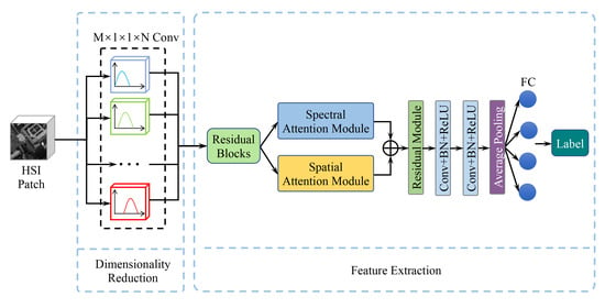
In our method, we also take advantage of CNN to learn feature representations of the scene. We use residual networks as a backbone network, followed by two attention modules, i.e., the spectral attention module and the spatial attention module. The spectral attention module is responsible for learning the correlation among spectral bands, and the spatial attention module considers the interdependencies between any two spatial pixels. Therefore, our model can effectively exploit both spectral and spatial features.

3. The Proposed Method

In this section, we first formulate the problem and introduce the motivation for our proposed method. Then, we describe our CSR optimization network and the feature extractor we use. Finally, learning details are provided. The overall framework of the proposed CSR-Net is illustrated in Figure 1.

3.1. Formulation and Motivation

Assuming that a hyperspectral camera is able to capture spectral images with M channels and N pixels, the obtained HSI H at the spatial position n for the m-th band can be described as

$$H_m\left(n\right)=\int c_m\left(\lambda \right)r(n,\lambda )\mathrm{d}\lambda ,$$

(1)

where $c_m\left(\lambda \right)$ denotes the CSR function along wavelength $\lambda$ for the m-th band. $r(n,\lambda )$ is the radiance of scene point at position n and wavelength $\lambda$, which is the compound of spectral reflectance and the illumination condition. Instead of using the continuous spectral bands, it is usually discretely described along spectra in practice, i.e., $\left\{{\lambda }_b\right\}$, where $1\le b\le B$ and B is the number of spectral bands. Thus, Equation (1) can be rewritten as

$$H_m\left(n\right)=\sum _{b=1}^B{c}_m\left({\lambda }_b\right)r(n,{\lambda }_b),$$

(2)

and it can be simplified in the matrix form as

$$\mathbf{H}=\mathbf{CR},$$

(3)

where $\mathbf{H}\in {\mathbb{R}}^{M\times N}$ denotes the matrix form of $H_m\left(n\right)$, $\mathbf{C}\in {\mathbb{R}}^{M\times B}$ and $\mathbf{R}\in {\mathbb{R}}^{B\times N}$ represent CSR and scene radiance, respectively. According to Equation (3), the captured hyperspectral data are determined by two factors, i.e., the CSR function $\mathbf{C}$ and the radiance of the scene $\mathbf{R}$. $\mathbf{R}$ is consistent for each scene when capturing outdoors or remotely sensed images. Since the spectral distribution of CSR depends on the type of camera, we could choose a proper $\mathbf{C}$ to influence the formation of $\mathbf{H}$ so as to retain more scene information for HSI classification.

Previous works on HSI recovery from a single RGB image [20,21] and HSI super-resolution [22] inferred that the abundant information of HSIs can be effectively kept in lower-dimensional data by using the optimal CSR. Here, we design a CNN architecture, i.e., CSR-Net, to learn the optimal CSR for the pixel-wise classification of HSI. Using the learned optimal CSR, we can capture images with much lower dimensions and the capturing process becomes convenient. The overview of our CSR-Net is shown in Figure 1. The CSR optimization layer and attention-based spectral–spatial feature extractor are described in the following sections.

3.2. CSR Optimization for Dimensionality Reduction

Existing CSR optimization methods [20,21,22] have proven that the optimal CSR function significantly improves the results of different HSI tasks. In this work, we aim to find the optimal CSR, which can be used to reduce data dimensions during the image acquisition process, and make the captured low-dimensional data contain sufficient spectral and spatial information for HSI classification tasks.

In the field of HSI classification, most previous works utilize hundreds of spectral bands as the model input. Due to the curse of dimensionality, dimensional reduction methods are presented to represent the complex HSIs by lower dimensional data. For example, Chen et al. [44] performed PCA on the input HSI before sending to a CNN, and Zhao et al. [45] proposed a balanced local discriminant embedding algorithm to extract features from high-dimensional HSIs. All these methods capture the full spectral bands and reduce their dimensions in the post-processing, and the main drawback is that the acquisition process is costly.

In this work, we present an approach to reduce the acquired image dimensions by optimizing CSR functions as well as guaranteeing the classification accuracy. Specifically, we propose a CSR optimization layer to create new CSR functions, so that data with lower dimensions are required and the classification accuracy is also kept in practice.

It can be observed from Equation (3) that each row of $\mathbf{C}$ is performing an exact convolution operation with $\mathbf{R}$ along spectral bands. Thus, it can be regarded as a $1\times 1$ convolutional layer. As illustrated on the left side of Figure 1, $\mathbf{C}$ can be replaced by $1\times 1$ convolution kernels with M output channels. Letting $\mathit{V}$ denote the corresponding convolutional layer, the process of capturing the t-th scene can be expressed as

$${\mathbf{H}}_t=\mathit{V}\ast {\mathbf{R}}_t,$$

(4)

where ${\mathbf{R}}_t$ is the radiance for the t-th scene.

Due to the limitation of CSR implementation technology, the designed CSR function should be smooth along the spectral dimension and all parameters in $\mathit{V}$ should be non-negative, for the camera always responds with a non-negative value. Thus, $\mathit{V}$ can be optimized through minimizing the empirical loss under smooth and non-negative constraints

$${\mathcal{L}}_c=\sum _{t=1}^T||\mathit{V}\ast {\mathbf{R}}_t-{\mathbf{Z}}_t{||}_2^2+\eta ||G\mathit{V}||,s.t.\mathit{V}\ge 0,$$

(5)

where ${\mathbf{Z}}_t$ denotes the corresponding ground truth for ${\mathbf{H}}_t$, and is the low dimensional data under the optimal CSR. $\eta$ is the predefined parameter, and G denotes the first derivative matrix for the penalty of non-smoothness.

In the training stage, the CSR optimization layer can simulate the capturing process of cameras and generate low-dimensional data. Then, the low-dimensional data are directly fed to the feature extractor (more details in Section 3.3). By optimizing the whole model, the optimal CSR for HSI classification is obtained. In the testing stage, thanks to the advanced filter technology, the learned CSR can be realized physically by optical filters. Our model makes it possible to capture fewer image bands in the data acquisition process and reduce the collection expenses to a great extent. As the learned CSR function contains prior knowledge of HSI classification, the captured low-dimensional data are sufficient for HSI classification. To better visualize the effect of our optimal CSR, we utilize a technique called t-SNE [46] to show the two-dimensional feature distributions from both the full HSI and the dimensionality-reduced image, which is captured under our optimal CSR, as shown in Figure 2. It can be observed that samples of different categories overlap a lot for the image without dimensionality reduction, while those samples become separable for the reduced image.

3.3. Deep Feature Extraction

To effectively extract the spatial and spectral features of the low dimensional images obtained by the optimal CSR, we employ the spectral attention module and spatial attention module to draw a global context over local features. Applying this architecture to pixel-wise HSI classification can help in the exploitation of spatial and spectral features, because the spectral attention module investigates the interdependencies between any two spectral maps and the spatial attention module exploits the global correlation between spatial pixel pairs.

The overview of the deep feature extraction network is shown on the right of Figure 1. We utilize an ordinary residual network as a backbone network. Specifically, a convolutional layer is performed to produce feature maps with P channels, and followed by K residual modules. In our experiment, we set $K=10$ and $P=256$. Each residual module has three convolutional layers, and the number of input and output channels are set as $a_0=a_2=P$, while the depth of the middle layer $a_1=P/4$, as shown in

Table 1. The architecture of the residual module $\mathcal{B}$.

Layer	Kernel Size	Padding	Stride
Conv1	$P/4\times 1\times 1\times P$	0	1
Batch Normalization
ReLU
Conv2	$P/4\times 3\times 3\times P/4$	1	1
Batch Normalization
ReLU
Conv3	$P\times 1\times 1\times P/4$	0	1
Batch Normalization
ReLU

. Thus, the output of the k-th residual module ${\mathbf{F}}_k\in {\mathbb{R}}^{P\times N}$ can be expressed as

$${\mathbf{F}}_k={\mathcal{B}}_k\left({\mathbf{F}}_{k-1}\right),$$

(6)

where ${\mathcal{B}}_k$ denotes the k-th residual module, and ${\mathbf{F}}_0$ is the input for the first residual block. After K residual modules, a feature map ${\mathbf{F}}_K$ is obtained.

The number of feature channels remains consistent through the residual blocks, and the output features still contain spatial and spectral correlation. The output of the K-th residual block ${\mathbf{F}}_K$ directly flows to two attention modules, i.e., the spectral attention module and spatial attention module, to exploit more global spectral and spatial correlation.

The spectral attention module is illustrated in Figure 3a. It learns a $P\times P$ attention map ${\mathbf{M}}_C$ along channels to improve the feature representation of spectral semantics, and the steps for obtaining spectral attention map are described as follows. First, we perform a matrix multiplication of ${\mathbf{F}}_K$ and the transpose of ${\mathbf{F}}_K$ to obtain a $P\times P$ tensor, which represents the interdependencies between every two feature channels. Then, a softmax layer is employed to rescale the spectral attention map between 0 and 1, the spectral attention map can be described as

$${\mathbf{M}}_C=softmax\left({\mathbf{F}}_K{\mathbf{F}}_K^T\right).$$

(7)

Then, by multiplying ${\mathbf{M}}_C$ and the original feature ${\mathbf{F}}_K$ and adding a skip connection, the correlations between every two feature channels are added to the original feature map, and we obtain features with more global semantics

$${\mathbf{E}}_C=\alpha {\mathbf{M}}_C{\mathbf{F}}_K+{\mathbf{F}}_K,$$

(8)

where $\alpha$ is a learnable variable.

Similar to the spectral attention module, as illustrated in Figure 3b, the spatial attention module obtains an attention map by performing a matrix multiplication of the transpose of ${\mathbf{F}}_K$ and ${\mathbf{F}}_K$

$${\mathbf{M}}_P=softmax\left({\mathbf{F}}_K^T{\mathbf{F}}_K\right),$$

(9)

and the map size is $N\times N$. It measures the mutual influence of any two spatial points. Thus, the output of the spatial attention module can be expressed as

$${\mathbf{E}}_P=\beta {\mathbf{M}}_P{\mathbf{F}}_K+{\mathbf{F}}_K,$$

(10)

where $\beta$ is learned with the whole architecture.

Then, the features from two attention modules are simply summed up and sent to a feature fusion residual block. We perform downsampling by two convolutional layers with a stride of 2, followed by batch normalization and ReLU [47], as well as an average pooling layer. Finally, the fused features are fed to a fully connected layer, which is the classifier of our model and outputs a category prediction. Since the final feature map considers both spectral and spatial correlation, it contains more discriminative features that are useful for HSI classification.

3.4. Learning Details

The learning framework mainly consists of two parts, i.e., a CSR optimization layer and a deep feature extractor. The output of the former part is directly fed to the latter part, and both parts are learned simultaneously.

Letting $\mathsf{\Theta }$ denote the parameter for our deep feature extraction network, the loss function for classification can be described as

$${\mathcal{L}}_f=\sum _{t=1}^{T}H(\widehat{g}({\mathbf{F}}_k^{\left(t\right)},\mathsf{\Theta }),g^{\left(t\right)}),$$

(11)

where $\widehat{g}$ and g represent the predicted label and ground truth label for the t-th scene, and H is the cross entropy loss to evaluate the classification accuracy.

When our model is trained, the loss for both the CSR layer and feature extractor are minimized simultaneously

$$\mathcal{L}=\tau {\mathcal{L}}_c+{\mathcal{L}}_f,$$

(12)

where $\tau$ is a predefined parameter.

In the experiment, through trial and error, we set $\eta =0.1$ and $\tau =1$ in Equations (5) and (12). Our network is optimized by the Stochastic Gradient Descent (SGD) [48] optimizer; the learning rate is initially set to $0.1$ and finally decays to $0.001$. The CSR optimization layer is initialized with random positive weights, and the feature extraction network is initialized by Kaiming initialization [49].

4. Experimental Results and Analysis

In this section, we first introduce four public HSI datasets used in our experiment and describe our experimental setting. Then, we present some analysis on CSR optimization. Finally, we compare our method with the state-of-the-art dimensionality reduction-based methods and feature-extraction methods.

4.1. Hyperspectral Datasets

In our experiment, four public remote-sensing datasets are used to evaluate all methods, i.e., the Indian Pines dataset, the University of Pavia dataset, the Salinas Valley dataset, and the Kennedy Space Center dataset.

Here, we provide more details of the datasets.

The University of Pavia dataset is captured by the ROSIS sensor in Pavia, Northern Italy. The whole image of the University of Pavia dataset contains $610\times 610$ pixels, with 103 spectral bands ranging from 430 to 860 nm, and the spatial resolution is $1.3$ m per pixel. As some part of this image is corrupted and contains no useful information, these parts are discarded and the size remains $610\times 340$ in practice. Each pixel in the University of Pavia dataset is labeled in 9 classes, and the sample numbers for each class is presented in

Table 2. Number of samples in the University of Pavia dataset.

Class No.	Color	Class Name	Samples
1		Asphalt	6631
2		Meadows	18649
3		Gravel	2099
4		Trees	3064
5		Painted metal sheets	1345
6		Bare Soil	5029
7		Bitumen	1330
8		Self-Blocking Bricks	3682
9		Shadows	947

.

The Indian Pines dataset is collected in north-western Indiana by the AVRIS sensor, and mainly consists of crops, forests and other natural perennial vegetation. The spatial size of the Indian Pines dataset is $145\times 145$, and it has 224 spectral bands ranging from 400 to 2500 nm. In our experiments, we use the corrected version of the dataset, which removes 24 bands over the region of water absorption. The ground truth is divided into 16 classes, and more details are shown in

Table 3. Number of samples in the Indian Pines dataset.

Class No.	Color	Class Name	Samples
1		Alfalfa	46
2		Corn-notill	1428
3		Corn-mintill	830
4		Corn	237
5		Grass-pasture	483
6		Grass-trees	730
7		Grass-pasture-mowed	28
8		Hay-windrowed	478
9		Oats	20
10		Soybean-notill	972
11		Soybean-mintill	2455
12		Soybean-clean	593
13		Wheat	205
14		Woods	1265
15		Buildings-Grass-Trees-Drives	386
16		Stone-Steel-Towers	93

.

The Salinas Valley dataset is also captured by AVRIS sensor, over Salinas Valley, which is the most productive agricultural region in California. The image size is $512\times 217$, with a high spatial resolution of $3.7$ m per pixel. The total number of spectral bands is 204 after removing 20 water absorption bands. The ground truth of the Salinas Valley dataset contains 16 classes, which is presented in

Table 4. Number of samples in the Salinas Valley dataset.

Class No.	Color	Class Name	Samples
1		Brocoli_green_weeds_1	2009
2		Brocoli_green_weeds_2	3726
3		Fallow	1976
4		Fallow_rough_plow	1394
5		Fallow_smooth	2678
6		Stubble	3959
7		Celery	3579
8		Grapes_untrained	11271
9		Soil_vinyard_develop	6203
10		Corn_senesced_green_weeds	3278
11		Lettuce_romaine_4wk	1068
12		Lettuce_romaine_5wk	1927
13		Lettuce_romaine_6wk	916
14		Lettuce_romaine_7wk	1070
15		Vinyard_untrained	7268
16		Vinyard_vertical_trellis	1807

.

The Kennedy Space Center dataset is acquired over the Kennedy Space Center, Florida, using the AVIRIS sensor. This dataset has a spatial resolution of 18 m per pixel, and consists of $512\times 614$ pixels in total. After removing some noisy and low-SNR bands, 176 bands are used in the experiments. The ground truth consists of 13 classes, and more details are provided in

Table 5. Number of samples in the Kennedy Space Center dataset.

Class No.	Color	Class Name	Samples
1		Scrub	761
2		Willow swamp	243
3		CP hammock	256
4		Slash pine	252
5		Oak/Broadleaf	161
6		Hardwood	229
7		Swamp	105
8		Graminoid marsh	431
9		Spartina Marsh	520
10		Cattail marsh	404
11		Salt Marsh	419
12		Mud flats	503
13		Water	927

.

4.2. Experimental Settings

For all four public remote-sensing datasets, we randomly select $15\%$ pixels as training samples, and the remained pixels are served as testing samples. For spectral-feature-extraction-based dimensionality reduction methods, the input is each $1\times 1$ pixel. As for spatial spectral-feature-extraction-based methods, the spatial size of the input patch infers the amount of neighboring information, and may influence the classification results. Therefore, we investigate the relationship between patch size and classification results. The classification results of our method using the patch size of $7\times 7$, $11\times 11$, $15\times 15$ and $19\times 19$ on these four datasets are provided in

Table 6. Quantitative classification results using different input patch sizes.

Dataset	Metrics	$7\times 7$	$11\times 11$	$15\times 15$	$19\times 19$
University of Pavia	OA (%)	$99.81$	$99.97$	$99.96$	$99.95$
	Kappa	$0.9974$	$0.9996$	$0.9995$	$0.9993$
Indian Pines	OA (%)	$96.43$	$99.23$	$99.52$	$99.64$
	Kappa	$0.9593$	$0.9915$	$0.9945$	$0.9949$
Salinas Valley	OA (%)	$99.81$	$99.97$	$99.96$	$99.97$
	Kappa	$0.9979$	$0.9997$	$0.9996$	$0.9996$
Kennedy Space Center	OA (%)	$97.67$	$99.30$	$99.89$	$99.98$
	Kappa	$0.9741$	$0.9922$	$0.9987$	$0.9997$

, and it can be observed that the accuracy becomes stable when the patch size is larger than $11\times 11$. Considering both the classification accuracy and computational cost, we choose a spatial size of $11\times 11$ for all spectral–spatial feature extraction methods.

In our experiments, all methods are evaluated by three widely used metrics, i.e., overall accuracy (OA), average accuracy (AA), and Kappa coefficient. Our experiments are run on an NVIDIA GTX 1080Ti GPU with the deep-learning framework PyTorch.

4.3. CSR Analysis

4.3.1. The Optimal CSR

To empirically analyze how our CSR optimization layer works, we present the spectral power distribution of the learned CSR under 10 spectral bands in Figure 4a. It can be seen that the combination of all spectra nearly cover the whole spectral bands, and some spectral bands with large weights can be considered as significant bands for HSI classification. This observation can be intuitively understood, since, for each component, capturing information independently could improve the utilization of feature channels. Covering all spectral bands retains the integral information of the scene. Some spectral bands contain more useful information for HSI classification, and these bands turn out to have larger weights. To further explain the optimal CSR, we compute the singular values for our optimal CSR function, and the result is shown in Figure 4b. Figure 4b further indicates the low linear correlation in optimal CSR.

4.3.2. The Curse of Dimensionality

It is known that the curse of dimensionality widely exists in HSI classification, and some classifiers show an apparent performance degradation as data dimensions become higher. Thus, it is significant for HSI classification methods to extract lower dimensional data before sending to the classifier. Besides, choosing a balanced number of dimensions is important, because high dimensions may cause the curse of dimensionality and images with too low dimensions (like RGB images) apparently contain less information. Thus, dimensionality reduction is introduced.

Since our CSR-based dimensionality reduction method reduces data dimensions in the spectral domain, we use spectral-feature-based HSI classification methods including SVM and 1D-CNN to verify the effectiveness of our optimal CSR on dimensionality reduction ability. We consider the spectral information for each pixel, and the spatial $1\times 1$ tensor is regarded as the model input. The results that use our CSR-based dimensionality reduction are denoted as CSR-SVM and CSR-1DCNN, and the OA and Kappa performances are shown in

Table 7. Results of SVM and 1D-CNN with and without CSR optimization.

Method	Dimension	University of Pavia		Indian Pines
		OA (%)	Kappa	OA (%)	Kappa
	10	$94.96$	$0.9331$	$82.87$	$0.8039$
	20	$95.01$	$0.9337$	$82.52$	$0.8003$
CSR-SVM	30	$95.32$	$0.9379$	$83.43$	$0.8106$
	40	$95.36$	$0.9384$	$83.68$	$0.8137$
	50	$95.47$	$0.9399$	$84.24$	$0.8200$
SVM	-	$93.61$	$0.9148$	$81.16$	$0.7841$
	10	$95.90$	$0.9456$	$87.80$	$0.8607$
	20	$95.72$	$0.9433$	$86.35$	$0.8443$
CSR-1DCNN	30	$95.84$	$0.9449$	$86.26$	$0.8431$
	40	$95.81$	$0.9444$	$86.01$	$0.8402$
	50	$95.94$	$0.9461$	$85.10$	$0.8300$
1D-CNN	-	$94.49$	$0.9269$	$84.09$	$0.8180$

. It can be seen that by using the low dimensional data that are captured by the optimal CSR, both methods achieve better classification results than when using the HSIs with full spectral bands. The reason for this is that the results using entire HSI as input suffer from the curse of dimensionality, and our CSR-optimization-based dimensionality reduction effectively avoids this phenomenon.

4.4. Compared with the State-of-the-Arts

4.4.1. Comparisons with Dimensionality Reduction Methods

First, we evaluate the effectiveness of our learned optimal CSR, compared with several famous dimensionality reduction methods, including Principle Component Analysis (PCA) [8], Locally Linear Embedding (LLE) [25], and Independent Component Analysis (ICA) [24]. Our dimensionality reduction method based on CSR optimization is denoted as CSR-Opt.

In the compared methods, PCA learns an orthogonal transformation to map the redundant data into a lower dimension space by maximizing the data variance. LLE is a manifold learning-based method that learns the compact representation of the high-dimensional data. ICA separates the data into additive non-Gaussian subcomponents. Our CSR-Opt attempts to find the best CSR by simulating camera sensors that could capture more informative images. To evaluate the dimensionality reduction ability, for CSR-Opt, the outputs of the CSR optimization layer are directly fed to the classifier without passing through the feature-extraction network.

We employ support vector machines (SVM) with RBF kernel to classify the low-dimensional features generated by the aforementioned methods, and the number of reduced dimensions are set from 10 to 50, at the interval of 10, for each method. Experiments are conducted on all four datasets mentioned in Section 4.1, and the corresponding OA and Kappa coefficients are shown in

Table 8. Quantitative classification results of dimensionality reduction methods on the University of Pavia dataset. The best results are highlighted in bold.

Dimension	Metrics	PCA	LLE	ICA	CSR-Opt
10	OA (%)	$89.62$	$77.64$	$87.54$	$\mathbf{94.91}$
	Kappa	$0.8600$	$0.6845$	$0.8314$	$\mathbf{0.9324}$
20	OA (%)	$93.32$	$82.69$	$92.36$	$\mathbf{95.34}$
	Kappa	$0.9107$	$0.7616$	$0.8979$	$\mathbf{0.9382}$
30	OA (%)	$93.35$	$85.57$	$91.93$	$\mathbf{95.20}$
	Kappa	$0.9111$	$0.8037$	$0.8923$	$\mathbf{0.9362}$
40	OA (%)	$93.36$	$86.44$	$91.24$	$\mathbf{95.30}$
	Kappa	$0.9111$	$0.8160$	$0.8831$	$\mathbf{0.9376}$
50	OA (%)	$93.40$	$87.65$	$90.52$	$\mathbf{95.41}$
	Kappa	$0.9118$	$0.8331$	$0.8736$	$\mathbf{0.9391}$

,

Table 9. Quantitative classification results of dimensionality reduction methods on the Indian Pines dataset. The best results are highlighted in bold.

Dimension	Metrics	PCA	LLE	ICA	CSR-Opt
10	OA (%)	$76.39$	$58.47$	$68.07$	$\mathbf{82.13}$
	Kappa	$0.7275$	$0.5033$	$0.6267$	$\mathbf{0.7958}$
20	OA (%)	$79.07$	$66.57$	$71.13$	$\mathbf{83.56}$
	Kappa	$0.7594$	$0.6092$	$0.6648$	$\mathbf{0.8123}$
30	OA (%)	$80.67$	$68.40$	$75.73$	$\mathbf{84.07}$
	Kappa	$0.7780$	$0.6317$	$0.7204$	$\mathbf{0.8180}$
40	OA (%)	$81.23$	$70.33$	$76.53$	$\mathbf{83.24}$
	Kappa	$0.7847$	$0.6561$	$0.7296$	$\mathbf{0.8088}$
50	OA (%)	$81.95$	$71.83$	$77.35$	$\mathbf{83.18}$
	Kappa	$0.7929$	$0.6752$	$0.7400$	$\mathbf{0.8079}$

,

Table 10. Quantitative classification results of dimensionality reduction methods on the Salinas Valley dataset. The best results are highlighted in bold.

Dimension	Metrics	PCA	LLE	ICA	CSR-Opt
10	OA (%)	$91.58$	$84.13$	$89.96$	$\mathbf{94.26}$
	Kappa	$0.9060$	$0.8219$	$0.8877$	$\mathbf{0.9360}$
20	OA (%)	$92.50$	$88.04$	$92.47$	$\mathbf{94.24}$
	Kappa	$0.9162$	$0.8665$	$0.9159$	$\mathbf{0.9358}$
30	OA (%)	$92.52$	$88.59$	$92.75$	$\mathbf{94.54}$
	Kappa	$0.9165$	$0.8726$	$0.9191$	$\mathbf{0.9392}$
40	OA (%)	$92.68$	$89.95$	$92.80$	$\mathbf{94.57}$
	Kappa	$0.9183$	$0.8877$	$0.9197$	$\mathbf{0.9395}$
50	OA (%)	$92.73$	$90.80$	$92.61$	$\mathbf{94.61}$
	Kappa	$0.9188$	$0.8972$	$0.9176$	$\mathbf{0.9399}$

and

Table 11. Quantitative classification results of dimensionality reduction methods on the Kennedy Space Center dataset. The best results are highlighted in bold.

Dimension	Metrics	PCA	LLE	ICA	CSR-Opt
10	OA (%)	$85.01$	$84.67$	$76.14$	$\mathbf{93.61}$
	Kappa	$0.8328$	$0.8290$	$0.7330$	$\mathbf{0.9288}$
20	OA (%)	$91.96$	$88.87$	$90.61$	$\mathbf{93.61}$
	Kappa	$0.9104$	$0.8759$	$0.8953$	$\mathbf{0.9288}$
30	OA (%)	$92.55$	$89.44$	$91.24$	$\mathbf{93.18}$
	Kappa	$0.9169$	$0.8822$	$0.9024$	$\mathbf{0.9241}$
40	OA (%)	$92.55$	$89.82$	$89.62$	$\mathbf{93.91}$
	Kappa	$0.9169$	$0.8865$	$0.8842$	$\mathbf{0.9321}$
50	OA (%)	$92.57$	$89.64$	$89.35$	$\mathbf{93.63}$
	Kappa	$0.9172$	$0.8846$	$0.8812$	$\mathbf{0.9291}$

. To better visualize this, we show the OA performances of all methods along feature numbers (ranging from 1 to 50) in Figure 5. It can be seen that PCA performs better than other traditional reduction methods. The reason for this is that PCA extracts more discriminative features, which help the classifier to make predictions. Our CSR-Opt shows better classification accuracy, compared to these traditional methods, and this verifies the effectiveness of our CSR optimization method for dimensional reduction. Moreover, from Table 8, Table 9, Table 10 and Table 11 and Figure 5, we can observe that the classification accuracy of our dimensionality reduction method improves significantly when we increase the number of dimensions from 1 to 10, while OA results are almost fixed using dimensions greater than 10. Other methods seem to require more dimensions to reach the saturated accuracy, e.g., 20 dimensions for PCA. In addition, our CSR optimization networks are simply implemented by convolutional layers, and the learned CSR can be further physically implemented to capture low-dimensional data in the acquisition process.

4.4.2. Comparisons with Feature Extraction Methods

We compare our feature extraction network with the optimal CSR to several feature extraction methods. The compared methods include Decision Tree (DT) [50], Logistic Regression (LR) [51], K-Nearest Neighbors (KNN) [52], 1D-CNN [12], 2D-CNN [44], 3D-CNN [44], as well as state-of-the-art deep-learning-based methods, i.e., VAD [18]. VAD proposes a two-branch visual attention-driven architecture to learn the mapping from input images to feature map. From Figure 5, we can observe that, as the number of dimensions increases from 1 to 10, the overall classification accuracy of our dimensionality reduction method improves remarkably. However, the accuracy becomes stable when the number of dimensions is more than 10, and using more dimensions could not achieve better results. In other words, 10 dimensions have kept enough information for HSI classification. Thus, we set the number of reduced dimensions to 10 for our CSR-Net.

We have conducted experiments on all datasets, and the average accuracy for each class, OA, AA and Kappa coefficients are shown in

Table 12. Quantitative classification results of feature extraction methods on the University of Pavia dataset. The best results are highlighted in bold.

Class No.	DT	LR	KNN	1D-CNN	2D-CNN	3D-CNN	VAD	CSR-Net
1	$86.94$	$92.02$	$88.75$	$93.49$	$97.45$	$98.33$	$99.89$	$\mathbf{100.00}$
2	$89.84$	$96.52$	$97.46$	$97.93$	$99.41$	$99.44$	$99.99$	$\mathbf{100.00}$
3	$60.48$	$75.06$	$68.16$	$75.56$	$95.13$	$95.13$	$99.44$	$\mathbf{99.94}$
4	$86.02$	$87.75$	$83.10$	$96.81$	$96.70$	$98.69$	$99.69$	$\mathbf{99.88}$
5	$97.29$	$98.95$	$98.60$	$99.83$	$\mathbf{100.00}$	$99.91$	$\mathbf{100.00}$	$\mathbf{100.00}$
6	$67.88$	$77.05$	$59.37$	$90.29$	$94.15$	$98.25$	$\mathbf{100.00}$	$\mathbf{100.00}$
7	$66.11$	$58.05$	$84.87$	$90.27$	$94.16$	$98.05$	$99.56$	$\mathbf{99.73}$
8	$75.59$	$87.41$	$85.59$	$90.10$	$95.46$	$97.99$	$99.94$	$\mathbf{99.84}$
9	$99.38$	$99.50$	$99.63$	$99.63$	$\mathbf{100.00}$	$\mathbf{100.00}$	$\mathbf{100.00}$	$99.88$
OA (%)	$83.58$	$90.01$	$87.84$	$94.35$	$97.61$	$98.72$	$99.91$	$\mathbf{99.96}$
AA (%)	$81.06$	$85.81$	$85.06$	$92.66$	$96.94$	$98.42$	$99.83$	$\mathbf{99.92}$
Kappa	$0.7821$	$0.8664$	$0.8354$	$0.9250$	$0.9683$	$0.9830$	$0.9988$	$\mathbf{0.9995}$

,

Table 13. Quantitative classification results of feature extraction methods on the Indian Pines dataset. The best results are highlighted in bold.

Class No.	DT	LR	KNN	1D-CNN	2D-CNN	3D-CNN	VAD	CSR-Net
1	$38.46$	$41.02$	$10.26$	$60.00$	$67.50$	$57.50$	$\mathbf{100.00}$	$92.31$
2	$53.38$	$75.86$	$57.66$	$81.80$	$83.61$	$90.77$	$\mathbf{99.84}$	$98.60$
3	$48.44$	$53.68$	$48.87$	$$78.61$$	$79.60$	$87.39$	$99.43$	$\mathbf{99.58}$
4	$42.29$	$42.29$	$38.81$	$66.34$	$74.75$	$79.21$	$97.51$	$\mathbf{100.00}$
5	$73.72$	$87.83$	$81.27$	$91.24$	$93.19$	$92.21$	$98.54$	$\mathbf{99.03}$
6	$80.81$	$95.65$	$98.23$	$97.26$	$97.58$	$98.87$	$99.68$	$\mathbf{99.84}$
7	$12.50$	$50.00$	$79.17$	$87.50$	$54.17$	$95.83$	$83.33$	$\mathbf{100.00}$
8	$89.90$	$98.77$	$98.28$	$99.26$	$98.77$	$99.01$	$\mathbf{100.00}$	$\mathbf{100.00}$
9	$23.52$	$58.82$	$17.64$	$47.06$	$88.24$	$\mathbf{100.00}$	$82.35$	$\mathbf{100.00}$
10	$55.93$	$63.43$	$69.85$	$87.91$	$88.51$	$91.90$	$97.58$	$\mathbf{98.43}$
11	$62.87$	$81.55$	$73.07$	$76.57$	$90.18$	$94.49$	$98.75$	$\mathbf{99.57}$
12	$36.71$	$57.54$	$27.57$	$83.37$	68.71	$87.92$	$\mathbf{99.01}$	$97.62$
13	$92.53$	$97.70$	$91.38$	$98.86$	$\mathbf{100.00}$	$96.57$	$\mathbf{100.00}$	$\mathbf{100.00}$
14	$83.16$	$95.91$	$94.79$	$94.70$	$95.26$	$96.47$	$98.98$	$\mathbf{99.91}$
15	$45.73$	$59.15$	$20.42$	$64.44$	$65.96$	$82.37$	$99.09$	$\mathbf{100.00}$
16	$75.95$	$83.54$	$83.54$	$72.50$	$91.25$	$\mathbf{100.00}$	$\mathbf{100.00}$	$96.2$
OA (%)	$63.02$	$77.54$	$70.34$	$84.00$	$87.43$	$92.56$	$98.96$	$\mathbf{99.24}$
AA (%)	$57.24$	$71.42$	$61.93$	$80.46$	$83.58$	$90.66$	$97.13$	$\mathbf{98.82}$
Kappa	$0.5793$	$0.7419$	$0.6580$	$0.8183$	$0.8566$	$0.9152$	$0.9881$	$\mathbf{0.9914}$

,

Table 14. Quantitative classification results of feature extraction methods on the Salinas Valley dataset. The best results are highlighted in bold.

Class No.	DT	LR	KNN	1D-CNN	2D-CNN	3D-CNN	VAD	CSR-Net
1	$97.42$	$99.47$	$98.36$	$92.83$	$99.59$	$98.24$	$\mathbf{100.00}$	$\mathbf{100.00}$
2	$99.15$	$99.97$	$99.56$	$99.81$	$99.68$	$99.97$	$\mathbf{100.00}$	$\mathbf{100.00}$
3	$96.01$	$97.26$	$99.29$	$98.51$	$99.88$	$99.76$	$\mathbf{100.00}$	$\mathbf{100.00}$
4	$97.81$	$99.83$	$99.75$	$99.66$	$99.83$	$\mathbf{99.92}$	$99.58$	$99.83$
5	$97.36$	$98.95$	$96.27$	$98.86$	$99.47$	$99.08$	$\mathbf{100.00}$	$\mathbf{100.00}$
6	$99.61$	$99.97$	$99.82$	$99.97$	$\mathbf{100.00}$	$99.94$	$\mathbf{100.00}$	$\mathbf{100.00}$
7	$99.38$	$99.74$	$99.05$	$99.67$	$\mathbf{100.00}$	$\mathbf{100.00}$	$\mathbf{100.00}$	$\mathbf{100.00}$
8	$74.91$	$89.02$	$82.13$	$90.29$	$90.12$	$87.16$	$99.93$	$\mathbf{99.98}$
9	$99.01$	$99.79$	$99.34$	$99.81$	$99.60$	$99.77$	$\mathbf{100.00}$	$\mathbf{100.00}$
10	$91.85$	$95.94$	$92.03$	$97.09$	$96.51$	$98.28$	$\mathbf{99.89}$	$\mathbf{99.96}$
11	$91.96$	$96.92$	$93.94$	$98.79$	$97.58$	$98.57$	$99.78$	$\mathbf{100.00}$
12	$98.05$	$99.88$	$99.88$	$99.82$	$99.94$	$98.96$	$\mathbf{100.00}$	$99.94$
13	$92.81$	$99.10$	$97.04$	$99.74$	$99.23$	$98.72$	$\mathbf{100.00}$	$\mathbf{100.00}$
14	$90.99$	$96.26$	$93.74$	$98.24$	$97.25$	$99.01$	$\mathbf{99.56}$	$\mathbf{99.56}$
15	$62.14$	$65.25$	$63.37$	$70.82$	$82.29$	$95.73$	$99.64$	$\mathbf{100.00}$
16	$95.83$	$98.18$	$97.98$	$98.89$	$99.54$	$95.51$	$\mathbf{100.00}$	$\mathbf{100.00}$
OA (%)	$87.86$	$92.36$	$90.05$	$93.57$	$95.10$	$96.23$	$99.91$	$\mathbf{99.98}$
AA (%)	$92.77$	$95.97$	$94.47$	$96.83$	$97.53$	$98.04$	$99.90$	$\mathbf{99.95}$
Kappa	$0.8649$	$0.9148$	$0.8892$	$0.9283$	$0.9455$	$0.9582$	$0.9990$	$\mathbf{0.9998}$

and

Table 15. Quantitative classification results of feature extraction methods on the Kennedy Space Center dataset. The best results are highlighted in bold.

Class No.	DT	LR	KNN	1D-CNN	2D-CNN	3D-CNN	VAD	CSR-Net
1	$85.01$	$95.36$	$93.20$	$95.05$	$97.06$	$98.30$	$\mathbf{100.00}$	$\mathbf{100.00}$
2	$75.36$	$77.78$	$83.57$	$88.89$	$81.64$	$88.89$	$99.03$	$\mathbf{100.00}$
3	$71.56$	$5.50$	$83.49$	$93.58$	$96.79$	$95.87$	$\mathbf{99.54}$	$\mathbf{99.54}$
4	$57.94$	$27.10$	$46.73$	$70.23$	$75.35$	$79.53$	$87.85$	$\mathbf{95.33}$
5	$53.28$	$0.00$	$45.99$	$75.91$	$73.72$	$74.45$	$97.08$	$\mathbf{99.27}$
6	$49.74$	$3.07$	$35.38$	6718	$66.15$	$91.79$	$99.49$	$\mathbf{100.00}$
7	$51.69$	$0.00$	$55.06$	$80.00$	$94.44$	$92.22$	$\mathbf{100.00}$	$\mathbf{100.00}$
8	$68.03$	$40.98$	$75.96$	$90.74$	$91.55$	$95.10$	$99.18$	$\mathbf{99.45}$
9	$84.16$	$86.20$	$89.59$	$95.24$	$94.12$	$99.55$	$\mathbf{100.00}$	$\mathbf{100.00}$
10	$78.43$	$81.34$	$79.01$	$96.22$	$95.35$	$95.64$	$\mathbf{100.00}$	$\mathbf{100.00}$
11	$98.03$	$91.01$	$96.35$	$97.76$	$\mathbf{100.00}$	$99.44$	$\mathbf{100.00}$	$\mathbf{100.00}$
12	$75.23$	$63.08$	$75.70$	$96.73$	$85.98$	$96.73$	$99.07$	$\mathbf{100.00}$
13	$98.98$	$98.98$	$98.10$	$99.75$	$97.84$	$99.87$	$\mathbf{100.00}$	$\mathbf{100.00}$
OA (%)	$79.98$	$68.58$	$81.81$	$92.33$	$91.56$	$95.55$	$99.07$	$\mathbf{99.68}$
AA (%)	$72.88$	$51.57$	$73.70$	$88.25$	88.46	$92.88$	$98.56$	$\mathbf{99.51}$
Kappa	$0.7773$	$0.6428$	$0.7969$	$0.9146$	$0.9061$	$0.9505$	$0.9897$	$\mathbf{0.9965}$

. It can be observed that traditional feature extraction methods like DT, LR and KNN can only provide limited classification accuracy. Among those deep-learning-based methods, deeper networks (VAD and Ours) tend to perform better than other architectures; this is because VAD and our method designed customized neural networks for hyperspetral images to consider both spatial and spectral correlation. Thus, the spatial and spectral correlation can be better utilized, and leads to better classification results. It can be noticed that our model outperforms all compared methods. Although VAD provides a close performance to our CSR-Net, our model does not need the full bands of HSI like VAD does, which are acquired by advanced and extremely expensive hyperspectral sensors. In the prediction process, instead of densely capturing the spectral information across full wavelength bands using costly devices, we only need to capture the low-dimensional data under the optimal CSR function. Our model can classify HSIs as accurately as other state-of-the-art architectures like VAD, with fewer input image bands.

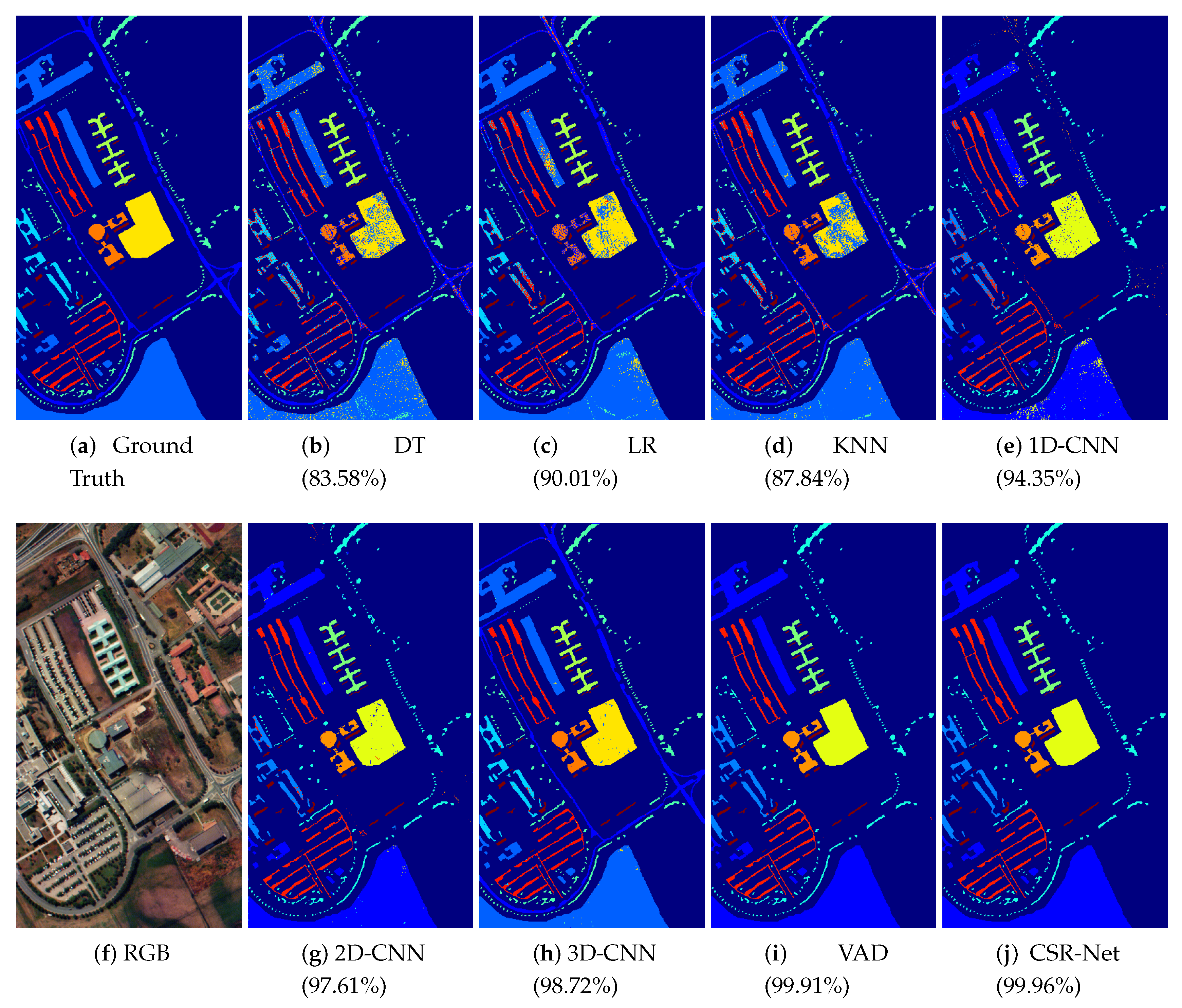
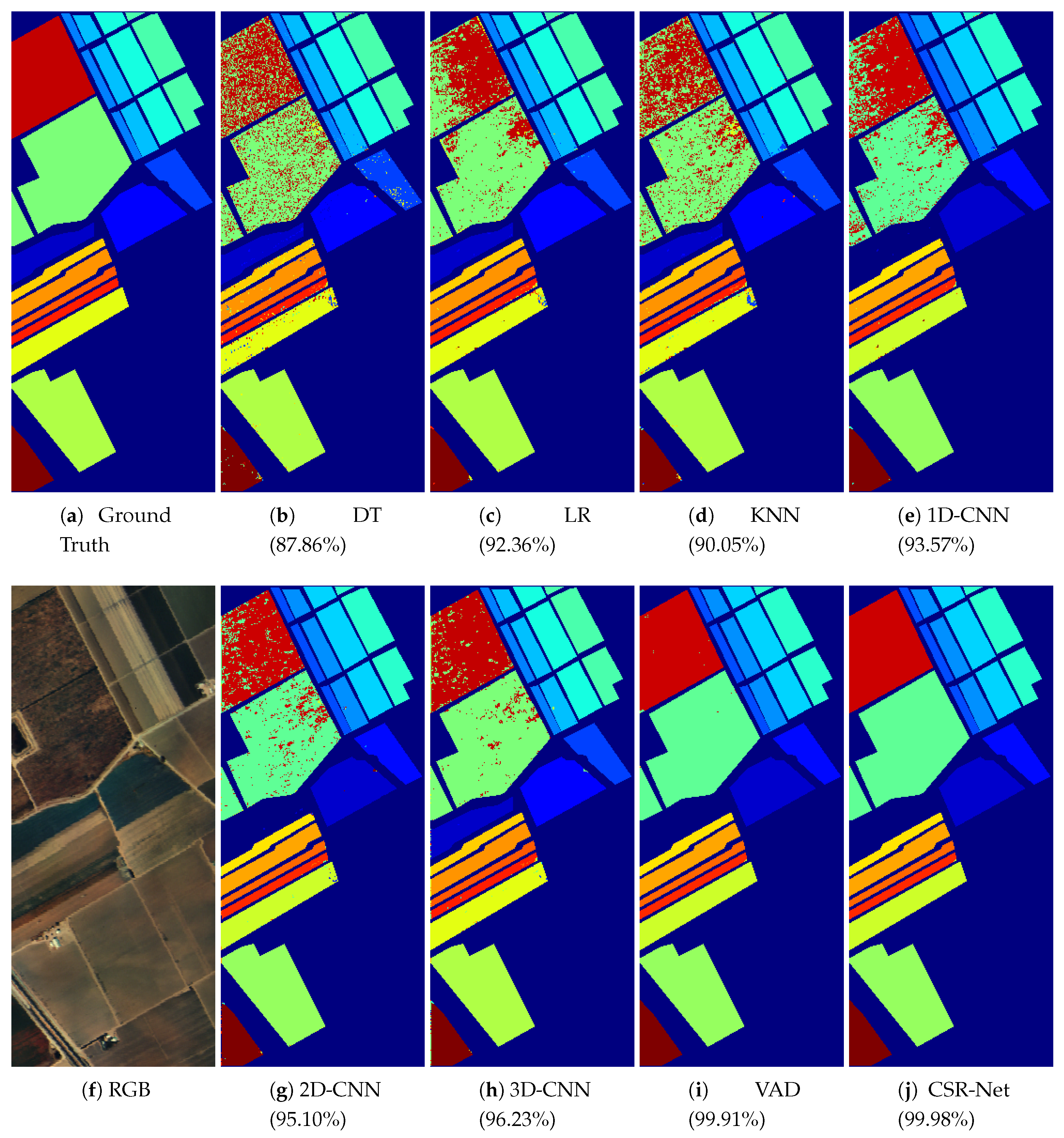
Figure 6, Figure 7, Figure 8 and Figure 9 show the classification map for all methods on the University of Pavia dataset, the Indian Pines dataset, the Salinas Valley dataset and the Kennedy Space Center dataset, respectively. It can be seen that the visual results of our methods are close to the ground truth, and the neighboring pixels are typically classified in the same class.

5. Conclusions

In this paper, we present a novel HSI classification method named the CSR-Net, which effectively investigates the optimal CSR and makes it possible to reach high classification accuracy with only limited number of image bands. Specifically, we design a special convolutional layer to simulate the camera-capturing process, which can guarantee the classification accuracy and effectively reduce the spectral dimensions of the captured data. Then, the reduced data are sent to spectral attention and spatial attention-based networks to extract the spectral–spatial correlation. Our CSR-Net can use far fewer bands than ordinary HSIs without sacrificing the classification accuracy, which makes it possible to simplify the data acquisition process, and provides insight into the design of simpler sensors to solve remote sensing problems. The experimental results of four HSI datasets verify the effectiveness of our method, and prove that the proposed method for low-dimensional data-capturing is sufficient for keeping enough information for HSI classification.

Our CSR optimization-based dimensionality reduction method sheds light on designing task-specific optical filters for different tasks, and can achieve promising results without capturing the redundant high-dimensional data. Therefore, the proposed optimal CSR-based method can further be applied to various practical situations. For example, in tje medical field, our CSR optimization model can be used for automatically finding the most suitable CSR, which can retain much diagnostic information with a limited number of data dimensions, which is meaningful for disease diagnosis and medical surgery. Applying our model in order to solve more practical problems remains one of our important future works.