Blind Unmixing of Hyperspectral Remote Sensing Data: A New Geometrical Method Based on a Two-Source Sparsity Constraint

Abstract

Blind source separation (or unmixing) methods process a set of mixed signals, which are typically linear memoryless combinations of source signals, so as to estimate these unknown source signals and/or combination coefficients. These methods have been extensively applied to hyperspectral images in the field of remote sensing, because the reflectance spectrum of each image pixel is often a mixture of elementary contributions, due to the limited spatial resolution of hyperspectral remote sensing sensors. Each spatial source signal then corresponds to a pure material, and its value in each pixel is equal to the “abundance fraction” of the corresponding Earth surface covered by that pure material. The mixing coefficients then form the pure material spectra. Various unmixing methods have been designed for this data model and the majority of them are either geometrical or statistical, or even based on sparse regressions. Various such unmixing techniques mainly consider assumptions that are related to the presence or absence of pure pixels (i.e., pixels which contain only one pure material). The case when, for each pure material, the image includes at least one pixel or zone which only contains that material yielded attractive unmixing methods, but corresponds to a stringent sparsity condition. We here aim at relaxing that condition, by only requesting a few tiny pixel zones to contain two pure materials. The proposed linear and geometrical sparse-based, blind (or unsupervised) unmixing method first automatically detects these zones. Each such zone defines a line in the data representation space. These lines are then estimated and clustered. The pairs of cluster centers, corresponding to lines, which have an intersection, yield the spectra of pure materials, forming the columns of the mixing matrix. Finally, the proposed method derives all abundance fractions, i.e., source signals, by using a least squares method with a non-negativity constraint. This method is applied to realistic synthetic images and is shown to outperform various methods from the literature. Indeed, and for the conducted experiments, when considering the pure material spectra extraction, the obtained improvements, for the considered spectral angle mapper performance criterion, vary between ${0.02}^{\circ }$ and ${12.43}^{\circ }$. For the abundance fractions estimation, the proposed technique is able to achieve a normalized mean square error lower than $0.01\%$, while the tested literature methods yield errors greater than $0.1\%$.

1. Introduction

Blind source separation (BSS) methods, also known as unsupervised unmixing methods in the field of “remote sensing” (Earth observation), aim at estimating a set of unknown source signals, called abundance fractions, and their corresponding endmember spectra, by using only a set of known observed signals (observed pixel spectra), obtained by combining these source signals by means of an almost unknown mixing function. Several algorithms have been proposed in the literature to this end.

These unmixing methods are based on a predefined mixing model. For some cases, depending on the application and/or the content of the used data, it can be linear or nonlinear. The linear model is the one that has most been used in the literature; therefore, we will focus on the methods based on this model which, in addition to its ease of use, is considered in some situations to represent a good approximation of the real environment [1]. Indeed, this model is adequate when considering large sets of land use presenting a more or less flat landscape (for example agricultural areas) and illuminated in a homogeneous way. Moreover, these methods use the assumptions related to the presence or absence of pure pixels in the considered image, or even according to the supervised nature or not, of the considered method. Based on works reported in [1,2], we present a classification of this type of method according to the presence or absence of pure pixels.

For the methods using the hypothesis of presence of pure pixels, the main assumption retained consists in assuming the existence of at least one pure pixel per distinct material contained in the considered image. Therefore, the natural adopted approach consists in finding the purest image pixels that are assumed to be located on the vertices of the simplex containing the observed data. Several strategies have been used to identify, as a first step, endmember spectra. To have a very precise idea of the most mentioned methods in the literature or other existing methods in this category (not cited in this paper), it is possible to consult, for example, with the works in [1,2,3,4] (and the associated references).

Despite the effectiveness of this type of method in the situation where there exist pure pixels, it does not give good results when applied to images that do not contain pure pixels [2]. Indeed, the hypothesis on which these methods are based is unfortunately not applicable to some remote sensing images whose spatial resolution is too low, for example, for them to be able to contain pure pixels. In this specific case, other geometrical approaches have been proposed which do not use this assumption. The majority of the methods developed in this category seek to generate virtual endmembers (which are not available in the considered image). In other words, this approach consists in minimizing the volume of the simplex containing the data. The approach adopted by these methods is considered to be a non-convex optimization problem, and is thus more difficult to solve in comparison with the approaches using pure pixels. To do this, here also, each of these methods has its own strategy. As for the previous category, more details concerning these methods, or other methods of the same category (not cited in this paper), are presented in [1,2,3,4] (and the associated references).

It is also possible to find in the literature other BSS-based approaches, namely, Independent Component Analysis, Non-negative Matrix Factorization, or Sparse Component Analysis. In particular, various BSS methods based on source sparsity may be found in the literature. They were developed for temporal, time-frequency, or even time-scale signal representations (for more details see in [5,6,7,8], and in particular in [9,10,11]). In [12], the same types of approaches as in [9] were applied to multispectral satellite images. As detailed in [12], the authors divide the observed data into small two-dimensional spatial zones, called “analysis zones”, consisting of adjacent pixels. These zones can be of any shape and are hereafter denoted as $\Omega$. The main hypothesis underlying these methods is related to the existence, in the considered image, of analysis zones containing only one “active” source, which means that each such analysis zone corresponds to a region of the Earth surface where only one pure material is present. Such a zone is called a “single-source zone” and each of its pixels is stated to be “pure”.

The advantage of such methods is that they require only a low sparsity hypothesis. However, the specific sparsity hypothesis underlying the approaches based on single-source zones is, as mentioned above, unfortunately not applicable to some images, whose spatial resolution is too low for them to contain pure pixels and therefore single-source zones. In this study, pure pixels are therefore ignored, which either means that they do not exist or that single-source zones are detected using, for example, the method proposed in [12], and the corresponding spectra are thus estimated by the latter method.

The above limitation led us to work with a less restrictive sparsity hypothesis than that presented above, and which consists in assuming the presence of “two-source zones”, i.e., zones containing only two pure materials. This assumption is quite realistic because we do not need pure pixels in the considered image. Furthermore, our unsupervised method estimates the endmember spectra without using a spectral library, which cannot be done for some semisupervised sparse based approaches reported in [1] (and the associated references).

To this end, we hereafter propose a new unsupervised unmixing approach, called “BiS-Corr”, for Bi-Source Correlation-based BSS method.

This method combines sparsity and geometrical properties. First, it consists of finding analysis zones containing only two sources, by using a criterion based on correlation. This step is followed by an identification step, where our method estimates the spectra of the pure materials contained in the considered image, thanks to geometrical properties. In the last step, our method estimates the abundance fractions of the pure materials by using a least squares method with non-negativity and sum-to-one constraints. The results obtained for realistic numerical mixtures of realistic sources prove the good performance of our method as compared with other methods from the literature.

The remainder of this paper is therefore organized as follows. We first define the standard linear mixing model for hyperspectral remote sensing images (Section 2). We then present some properties that facilitate the introduction of the hypotheses considered in the proposed BSS method (Section 3). This method is detailed in Section 4, and we provide details about the data used in our experiments (Section 5), test results in Section 6, and finally a discussion of the obtained results in Section 7, before a conclusion.

2. Data Model

In this paper, the considered hyperspectral remote sensing image is represented by using the standard linear mixing model. This model is here presented in the same way as in [1,13]. After vectorizing the spatial dimensions, one can express the non-negative reflectance observed in the ℓth spectral band of the image, for a given pixel n, as follows,

$$x_{\ell }(n)=\sum _{m=1}^M{r}_{\ell m}{f}_m(n)\forall n\in \left\{1\cdots N\right\},\ell \in \left\{1\cdots L\right\}$$

(1)

where $r_{\ell m}$ represents the ℓth spectral component (reflectance) of the mth pure material. $f_m(n)$ represents the abundance fraction of the mth pure material in the nth pixel. M is the number of pure materials in the considered image, N is its number of pixels, and L is its number of spectral bands.

The complete observed image is defined as

$$X=\left[\mathbf{x}(1)\cdots \mathbf{x}(N)\right]$$

(2)

with

$$\mathbf{x}(n)={\left[x_1(n)\cdots x_L(n)\right]}^T,$$

(3)

where ${}^T$ stands for transpose. Using (1), this image reads

$$X=RF,$$

(4)

where the columns of the mixing matrix R contain the (non-negative) spectra of the pure materials, that is

$$R=\left[{\mathbf{r}}_1\cdots {\mathbf{r}}_M\right]$$

(5)

with

$${\mathbf{r}}_m={\left[r_{1m}\cdots r_{Lm}\right]}^T.$$

(6)

Moreover, each column of the source matrix F contains the abundance fractions of all the pure materials in the considered pixel. It is thus organized as follows,

$$F=\left[\mathbf{f}(1)\cdots \mathbf{f}(N)\right]$$

(7)

with

$$\mathbf{f}(n)={\left[f_1(n)\cdots f_M(n)\right]}^T.$$

(8)

Besides, these data meet the following non-negativity and sum-to-one constraints,

$$f_m(n)\ge 0,\forall \begin{array}{c}m\in \left\{1\cdots M\right\}\\ n\in \left\{1\cdots N\right\},\end{array}$$

(9)

$$\sum _{m=1}^M{f}_m(n)=1,\forall n\in \left\{1\cdots N\right\}.$$

(10)

3. Properties of Two-Source Analysis Zones

In the proposed approach, we first focus on the pixels containing only two sources of indices i and j (with $i\ne j$) among the M sources taken into account in the considered data. Each such pixel is hereafter referred to as a “two-source pixel”. Due to (1), such a pixel yields

$$x_{\ell }(n)=r_{\ell i}{f}_i(n)+r_{\ell j}{f}_j(n).$$

(11)

Considering (11), and taking into account the constraint (10),which induces $f_j(n)=1-f_i(n)$, we obtain

$$x_{\ell }(n)=f_i(n)[r_{\ell i}-r_{\ell j}]+r_{\ell j}.$$

(12)

If we now use two spectral bands of indices ℓ and p (with $\ell \ne p$), for each pixel n we obtain a couple of values ($x_{\ell }(n)$, $x_p(n)$) defining a point in the ($x_{\ell }$, $x_p$) plane. The totality of the two-source pixels containing the selected sources i and j defines a scatter plot in this plane, and we want to analyze the shape of this scatter plot. Taking (12) and its counterpart for band p into account, we have

$$\begin{array}{ccc}\hfill x_{\ell }(n)-r_{\ell j}& =& f_i(n)[r_{\ell i}-r_{\ell j}]\hfill \end{array}$$

(13)

$$\begin{array}{ccc}\hfill x_p(n)-r_{pj}& =& f_i(n)[r_{pi}-r_{pj}],\hfill \end{array}$$

(14)

which yields

$$f_i(n)[r_{pi}-r_{pj}][x_{\ell }(n)-r_{\ell j}]=f_i(n)[r_{\ell i}-r_{\ell j}][x_p(n)-r_{pj}].$$

(15)

Assume that only two sources $f_i(n)$ and $f_j(n)$ are non-null everywhere in an analysis zone (hereafter called a “two-source zone”) composed of adjacent pixels. In this case, Equation (15) yields the following expression for the second coordinate of the ($x_{\ell }$, $x_p$) point with respect to the first one,

$$x_p(n)=a{x}_{\ell }(n)+r_{pj}-a{r}_{\ell j},$$

(16)

with

$$a=\frac{r_{pi}-r_{pj}}{r_{\ell i}-r_{\ell j}},$$

(17)

assuming

$$r_{\ell i}\ne r_{\ell j}.$$

(18)

Thus, all the corresponding points ($x_{\ell }(n)$, $x_p(n)$) belong to the above-defined line (16). On the contrary, if more than two sources are non-zero and vary arbitrarily in an analysis zone, the corresponding points are not on a line.

More precisely, the two-source points only belong to a segment of the above line, as $0\le f_i(n)\le 1$. The bounds of this segment are therefore defined by

(i)

$f_i(n)=0$:

In this case, Equations (13) and (14) yield $x_{\ell }(n)=r_{\ell j}$ and $x_p(n)=r_{pj}$, respectively. This is normal, because only source j is non-zero, and it is its spectrum that is observed in such a pixel.

(ii)

$f_i(n)=1$:

In this case, $x_{\ell }(n)=r_{\ell i}$ and $x_p(n)=r_{pi}$, which is interpreted in the same way as above.

If we now assume that the considered image contains at least one two-source analysis zone for each pair of sources, among the M sources in that image, then a line segment is obtained for each possible pair of sources. We then have a total of $\frac{M(M-1)}{2}$ possible line segments. These segments have common extremities corresponding to the M sources. As shown above, each of these extreme points has the following coordinates, $(r_{\ell m},r_{pm})$ with $m\in \left\{1\cdots M\right\}$.

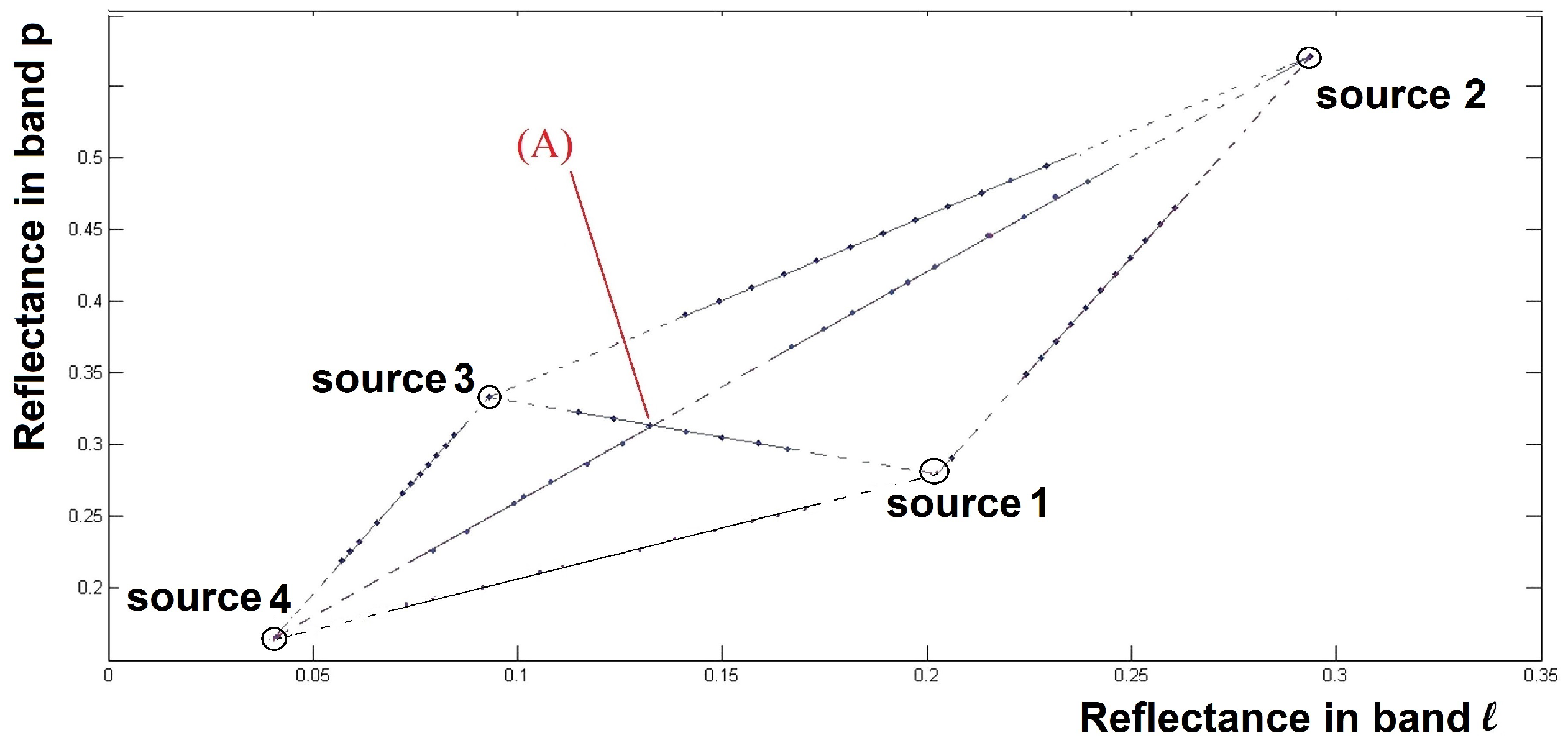
Figure 1 shows a scatter plot obtained for pixels corresponding to all the pairs of sources selected from an overall set of $M=4$ artificial sources inducing, as mentioned above, $\frac{M(M-1)}{2}=6$ possible lines.

The most difficult case, which is therefore investigated in this paper, is when the available data points that are associated with each pair of sources do not include the bounds of each possible segment. These segment bounds correspond to pure pixels, and are illustrated by small circles in Figure 1.

In the case when there are no pure pixels, assume we managed to estimate two lines corresponding to two pairs of sources, with indices $[i,j]$ for the first pair and $[j,k]$ for the second (with $i\ne k$). This means that we estimated the slopes and intercepts of both lines. Assuming that these lines are not identical for the considered two spectral bands, this allows us to deduce their intersection point and thus obtain the coordinates ($r_{\ell j},r_{pj}$), corresponding to spectral bands l and p of the $j^{th}$ pure material.

The above detailed analysis, which considers only two spectral bands, is useful to understand the preliminary version of our approach. However, the use of only two bands does not allow us to completely solve the considered problem. This is first because the obtained intersection points for all the pairs of sources only give us a part of the spectra that corresponds to two spectral bands (among the L bands considered in the image); second, this 2D scatter plot also contains spurious intersections, or intersections between line segments associated with pairs of sources $[i,j]$ and $[i^{\prime },j^{\prime }]$ which share no source: such intersections do not correspond to any actual pure material. This case is represented by point (A) of Figure 1. Blind determination of all the intersections of two-source segments would therefore lead to spurious pure materials. This problem results from the fact that two (non-parallel) lines always intersect in a 2D space.

To solve the above problem, we now extend our approach to more than two spectral bands. To this end, we first estimate the parameters of the lines associated with each two-source zone, we then classify these parameters, we determine the intersection points which provide pure spectra estimates, and finally we estimate the abundance fractions. This yields the complete version of our BSS method, which is more formally presented in the next section.

4. Proposed BSS Method (BiS-Corr)

Using the properties introduced above, we hereafter define a new BSS method (called BiS-Corr) based on sparsity and applied to hyperspectral remote sensing images. In this approach, we use some notations, definitions, and assumptions that are related to the sought sources (abundance fractions) and mixing matrix (reflectance spectra of pure materials). These items are detailed below.

Notations:

• The zero-mean versions of $x_l(n)$ and $f_m(n)$ are respectively denoted as follows,

  $$\begin{array}{ccc}\hfill {\overline{x}}_l(n)& =& x_l(n)-{\mu }_{x_l}\hfill \\ \hfill {\overline{f}}_m(n)& =& f_m(n)-{\mu }_{f_m},\hfill \end{array}$$

  where ${\mu }_{x_l}$ and ${\mu }_{f_m}$, respectively, represent the means of $x_l(n)$ and $f_m(n)$ over the considered analysis zone $\Omega$.
• The vector ${\mathbf{x}}_{\ell }(\Omega )$ is formed of all $x_{\ell }(n)$ with $n\in \Omega$, when considering $\Omega$ as a set of indices of the associated pixels.
• The vector ${\mathbf{f}}_m(\Omega )$ is formed of all $f_m(n)$ with $n\in \Omega$.
• The zero-mean versions of the vectors ${\mathbf{x}}_{\ell }(\Omega )$ and ${\mathbf{f}}_m(\Omega )$ are, respectively, denoted as ${\overline{\mathbf{x}}}_{\ell }(\Omega )$ and ${\overline{\mathbf{f}}}_m(\Omega )$.

Definition 1.

A pure material, with an index i among the M considered pure materials, is “active“ in an analysis zone Ω if it yields a non-zero vector ${\mathbf{f}}_i(\Omega )$.

Definition 2.

A pair of pure materials is “isolated” in an analysis zone if only these two pure materials are active in this analysis zone. This zone is then called a “two-source zone”.

Definition 3.

A pair of pure materials is said to be “accessible” in the spatial domain if there exists at least one analysis zone wherein this pair of materials is isolated.

Assumption 1.

If a pure material, with an index i among the M considered pure materials, is active in an analysis zone Ω, then its abundance fraction $f_i(n)$ is not constant over all that zone (so that ${\overline{\mathbf{f}}}_i(\Omega )\ne 0$).

Assumption 2.

For each pure material of index j, among the M considered pure materials, there are at least two pairs of materials with indices $[i,j]$ and $[j,k]$ (with $i\ne k$), sharing this material, which are accessible.

Using the sum-to-one constraint (10), we can write one of the sources (among the M sources considered in the mixture) with respect to the others. The index of this arbitrary source is denoted as $m_0$, and we denote as ${\mathcal{M}}_0$ the set of indices of all the other sources:

$${\mathcal{M}}_0=\left\{1\cdots M\right\}-\left\{m_0\right\}.$$

(19)

Equation (10) thus yields

$$f_{m_0}(n)=1-\sum _{m\in {\mathcal{M}}_0}{f}_m(n).$$

(20)

By inserting (20) in (1), we obtain

$$x_{\ell }(n)=\sum _{m\in {\mathcal{M}}_0}{r}_{\ell m}{f}_m(n)+r_{\ell m_0}\left[1-\sum _{m\in {\mathcal{M}}_0}{f}_m(n)\right],$$

(21)

with $r_{\ell m_0}\left[1-{\sum }_{m\in {\mathcal{M}}_0}{f}_m(n)\right]$ representing the term related to source $m_0$ that we wish to remove, so as to consider only the sources contained in ${\mathcal{M}}_0$. Equation (21) thus yields

$$x_{\ell }(n)=\left[\sum _{m\in {\mathcal{M}}_0}(r_{\ell m}-r_{\ell m_0})f_m(n)\right]+r_{\ell m_0}.$$

(22)

Using the above-defined notations, the centered and vectorized version of (22) reads

$${\overline{\mathbf{x}}}_{\ell }(\Omega )=\sum _{m\in {\mathcal{M}}_0}(r_{\ell m}-r_{\ell m_0}){\overline{\mathbf{f}}}_m(\Omega ).$$

(23)

Similarly, as regards the spectral band p, we obtain

$${\overline{\mathbf{x}}}_p(\Omega )=\sum _{m\in {\mathcal{M}}_0}(r_{pm}-r_{p{m}_0}){\overline{\mathbf{f}}}_m(\Omega ).$$

(24)

In the case when more than two pure materials are active in the considered analysis zone $\Omega$, the set ${\mathcal{M}}_0$ contains at least two active pure materials. To handle this configuration, we also add the following assumptions, where $M(\Omega )$ is the number of pure materials that are active in zone $\Omega$:

Assumption 3.

In each analysis zone Ω where $M(\Omega )$ is greater than or equal to three, when considering up to $M(\Omega )$ non-zero vectors ${\overline{\mathbf{f}}}_m(\Omega )$, they are always linearly independent.

Assumption 4.

In each analysis zone Ω, the “matrix of reflectance differences” has full column rank, where this matrix is defined as follows. Each of its columns corresponds to a value $m\in {\mathcal{M}}_0$ such that ${\overline{\mathbf{f}}}_m(\Omega )$ is non-zero. This column contains the values $(r_{\ell m}-r_{\ell m_0})$ corresponding to all spectral bands ℓ.

Assumption 5.

The mixing model is locally (over)determined, $L\ge M(\Omega )$ in any analysis zone Ω (see [12] for more details).

Taking into account these assumptions and definitions, we now present the general structure of the proposed approach. It consists of the following three steps.

• Detection of all the two-source analysis zones that are available in the observed image.
• Identification of the mixing matrix.
• Extraction of the sought sources, taking the non-negativity constraint into account.

Each of these steps is detailed below.

4.1. Two-Source Zone Detection Step (Step 1)

The observed data are first divided into small two-dimensional spatial zones (analysis zones), consisting of adjacent pixels. The spatial domain is then explored using these analysis zones, which are adjacent or overlapping. The purpose of this step is to determine the analysis zones of the image where only two pure materials are active. These represent the sought two-source zones.

In any two-source zone, using the zero-mean versions of the observed data in bands ℓ and p, (13) and () yield

$$\begin{array}{ccc}\hfill {\overline{\mathbf{x}}}_{\ell }(\Omega )& =& (r_{\ell i}-r_{\ell j}){\overline{\mathbf{f}}}_i(\Omega )\hfill \end{array}$$

(25)

$$\begin{array}{ccc}\hfill {\overline{\mathbf{x}}}_p(\Omega )& =& (r_{pi}-r_{pj}){\overline{\mathbf{f}}}_i(\Omega ).\hfill \end{array}$$

(26)

Equations (25) and (26) show that ${\overline{x}}_{\ell }(n)$ and ${\overline{x}}_p(n)$ vary proportionally over the two-source zones. For each analysis zone $\Omega$, we detect this proportionality through the calculation of the cross-correlation coefficients ${\rho }_{x_{\ell }{x}_p}(\Omega )$, between the (centered) observed signals, which are defined as follows,

$${\rho }_{x_{\ell }{x}_p}(\Omega )=\frac{〈{\overline{\mathbf{x}}}_{\ell }(\Omega ),{\overline{\mathbf{x}}}_p(\Omega )〉}{∥{\overline{\mathbf{x}}}_{\ell }(\Omega )∥·∥{\overline{\mathbf{x}}}_p(\Omega )∥}\forall \ell ,p\in \left\{1\cdots L\right\}\mathrm{and}\ell >p,$$

(27)

where $∥x∥$ and $〈x,y〉$, respectively, represent the 2-norm of x and inner product of x and y.

Applying the Cauchy–Schwarz inequality to (27), shows that

$$|{\rho }_{x_{\ell }{x}_p}(\Omega )|\le 1,\forall \ell ,p\in \left\{1\cdots L\right\}\mathrm{and}\ell >p,$$

(28)

with equality if and only if ${\overline{\mathbf{x}}}_{\ell }(\Omega )$ and ${\overline{\mathbf{x}}}_p(\Omega )$ are linearly dependent. Thus, a necessary condition for a pair of materials to be isolated in an analysis zone $\Omega$ is

$$\left|{\rho }_{x_{\ell }{x}_p}(\Omega )\right|=1\forall \ell ,p\in \left\{1\cdots L\right\}\mathrm{and}\ell >p,$$

(29)

because if, in the considered zone, the number of active pure materials is equal to two, Equations (25) and (26) show that ${\overline{\mathbf{x}}}_{\ell }(\Omega )$ and ${\overline{\mathbf{x}}}_p(\Omega )$ are linearly dependent, and therefore the values of $|{\rho }_{x_{\ell }{x}_p}(\Omega )|$ reach their maximum, equal to one. Furthermore, under Assumptions 3 and 4, condition (29) is a sufficient condition for the considered analysis zone to be two-source, as shown in the Appendix A.

In practice, for each zone, to check if (29) is met, we compute the minimum among all $|{\rho }_{x_{\ell }{x}_p}(\Omega )|$ for any ℓ, p with $\ell >p$. If this measure is greater than a threshold set to a value somewhat lower than one, we consider this zone as a two-source zone.

4.2. Identification Step (Step 2)

This step consists in estimating the columns of the mixing matrix. To this end, we first estimate the parameters of each line associated with a two-source zone, supposedly present in the considered data (Part 1). The vectors of parameters thus obtained are then clustered, so as to derive a single line for each considered pair of sources (Part 2). Finally, the minimum distance between lines is calculated for each pair of these lines, so as to then derive the coordinates of the sought pure material spectra (or endmember spectra).

4.2.1. Line Parameter Estimation (Part 1)

In the L-dimensional space associated with each data point defined by a pixel spectrum of the observed hyperspectral image, a line D may be represented by the parametric equation [14,15,16]

$${\mathbf{p}}_s=s\mathbf{u}+\mathbf{d},$$

(30)

where ${\mathbf{p}}_s$, $\mathbf{u}$, and $\mathbf{d}$ are L-dimensional column vectors and s is a scalar. In an ideal two-source zone containing sources i and j, all points corresponding to observed spectra belong to such a line: their spectra read as ${\mathbf{p}}_s$ in (30), where the ℓth components of $\mathbf{u}$ and $\mathbf{d}$ are, respectively, equal to $[r_{\ell i}-r_{\ell j}]$ and $r_{\ell j}$, and where s is equal to $f_i(n)$. In practice, two-source zones are only nearly ideal, and the data points associated with such a zone are only nearly aligned. In this Part 1, we therefore aim at estimating the direction vector $\mathbf{u}$ and the point represented by the vector $\mathbf{d}$ of the line D, which minimizes the mean-squared error between the data points of the considered zone and this line.

Each analysis zone $\Omega$ provides a matrix $X(\Omega )$ containing the pixel values $x_{\ell }(n)$ of the considered zone, in its column ℓ (with $\ell \in \left\{1\cdots L\right\}$). One of the possible solutions to fitting a line to data points is to determine the first principal axis of these data [14,15]. This is achieved as follows.

• Determination of the vector $\mathbf{d}$ of Equation (30), by calculating the mean of the columns of $X^T(\Omega )$. The obtained vector corresponds to the center of gravity of these data.
• Determination of vector $\mathbf{u}$ which is nothing but the eigenvector associated with the largest eigenvalue of the covariance matrix of $X(\Omega )$.

However, when fitting a model to data, it is important that the model is identifiable. Otherwise, the solution of the fitting procedure is not unique. In (30), the line is defined by $2L$ parameters: the components of u and d. However, in an L-dimensional space, a line can be characterized as follows with only $(2L-2)$ parameters (This is easier to understand if we apply our reasoning in a 2 dimensional space ($L=2$). Indeed, although in this case the line (30) is defined by $2L$ ($=4$) parameters, in reality there are only $2L-2$ ($=2$) degrees of freedom (slope and intercept).), provided it is not orthogonal to the first axis, i.e., provided the first component $u_1$ of u is different from zero. The 1st and ℓth elements of (30) read

$$p_1=s{u}_1+d_1\mathrm{and}{p}_{\ell }=s{u}_{\ell }+d_{\ell },\mathrm{with}\ell =\left\{2\cdots L\right\}.$$

Thus, if $u_1\ne 0$, we obtain

$$\frac{p_1-d_1}{u_1}=\frac{p_{\ell }-d_{\ell }}{u_{\ell }}=s,$$

which yields

$$p_{\ell }=\frac{u_{\ell }}{u_1}{p}_1+d_{\ell }-\frac{u_{\ell }}{u_1}{d}_1,$$

that is

$$p_{\ell }={u_{\ell }}^{*}{p}_1+{d_{\ell }}^{*},$$

(31)

where the $(2L-2)$ normalized parameters are defined as follows,

$${u_{\ell }}^{*}=\frac{u_{\ell }}{u_1}\mathrm{and}{d_{\ell }}^{*}=d_{\ell }-\frac{u_{\ell }}{u_1}{d}_1.$$

(32)

Equations (31) and (32) also apply to $\ell =1$, by introducing ${u_1}^{*}=1$ and ${d_1}^{*}=0$. Gathering all the L components ${u_{\ell }}^{*}$ (respectively, ${d_{\ell }}^{*}$) in a vector ${\mathbf{u}}^{*}$ (respectively, ${\mathbf{d}}^{*}$), Equation (31) defining the considered line reads in vector form

$${\mathbf{p}}_{s^{*}}=s^{*}{\mathbf{u}}^{*}+{\mathbf{d}}^{*},\mathrm{with}{s}^{*}=p_1.$$

For the sake of readability, $s^{*}$ is replaced by s hereafter (particularly in Part 3).

4.2.2. Classification of the Line Parameters (Part 2)

For each pair of sources, the above Part 1 allows one to define several couples of vectors ${\mathbf{u}}^{*}$ and ${\mathbf{d}}^{*}$, i.e., one couple for each two-source zone containing these sources. We then aim at deriving a single couple $({\mathbf{u}}^{*},{\mathbf{d}}^{*})$ for each pair of sources. In other words, the current Part 2 consists in classifying the different two-source zones that were previously determined, taking into account the parameters of the corresponding lines, thereby permitting the identification of a unique line associated with each pair of sources. To this end, we rearrange each estimated couple $({\mathbf{u}}^{*},{\mathbf{d}}^{*})$ as an overall vector and we classify these vectors by successively using each of them as follows.

After setting the first vector to a first class denoted as “class-1”, each vector is compared to that attributed to this class by computing the distance between them (the 2-norm of their difference). Whenever this distance is less than a threshold, we assign the tested vector to this first class. Otherwise, a new class is created (“class-2”), and we assign this vector to it. Then, we compare the subsequent vectors to the first vector of each of the existing classes. Each tested vector is either assigned to the closest class in terms of distance, or if its distance to all existing classes is greater than the fixed threshold, it defines a new class, and so on for all other vectors.

After thus assigning a class to each vector, we estimate a unique line for each class, by repeating the line parameter estimation procedure described in Part 1, the only difference being the use of a new matrix containing the pixel values corresponding to all two-source zones detected for the considered class, to increase accuracy.

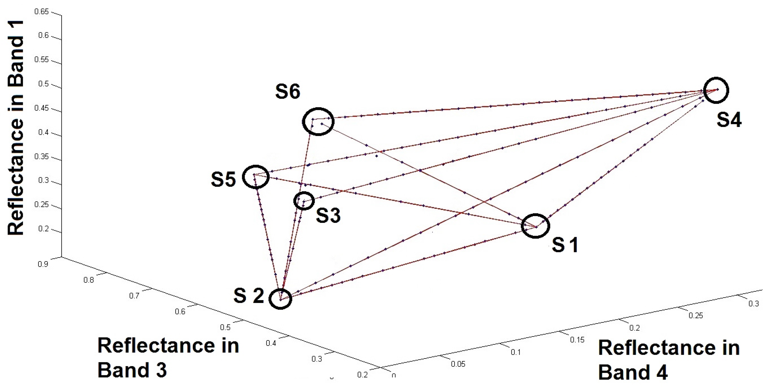
Figure 2 shows an illustration of several lines corresponding to different classes. These lines were defined from a simulated image containing 6 artificial sources. As mentioned earlier in Section 3, the number of possible lines is 15 (calculated from $\frac{M(M-1)}{2}$).

The number of lines corresponding to the determined pairs of sources (Although the number of lines determined by the procedure detailed above is less than the number of possible lines given the number of sources used in this example, it is still possible, with the assumptions listed above, to find the sought sources. As an example, even if the method could not detect the line “$s_1{s}_3$” because the considered image does not contain two-source zones for sources $s_1$ and $s_3$, source $s_3$ can be identified, as shown in Figure 2, from the (detected) lines “$s_2{s}_3$” and “$s_3{s}_4$”.) in this example is 11.

As illustrated in Figure 2, at this stage of the proposed method, we are able to represent each line containing the points associated with each class, and thus to estimate the points of intersection between different pairs of lines (the small circles in Figure 2). This is detailed below.

4.2.3. Computing the Minimum-Distance Points between Lines (Part 3)

In this last part of the identification step, the coordinates of each endmember spectrum (column of the mixing matrix R) are derived by estimating the intersection points, successively for different pairs of lines corresponding to two pairs of sources. In theory, such points exist if and only if the considered two pairs of sources share one source, under the following assumption (which is not very restrictive in our applications).

Assumption 6.

If two pairs of pure materials do not contain a common pure material, the two lines, respectively defined by each of these pairs on their two-source zones, do not have any intersection point.

However, in practice, two lines estimated for two pairs of pure materials containing a common material may not exactly intersect (for example, due to data noise). In this case, the endmember spectra coordinates may be estimated by computing the closest point, i.e., the minimum-distance one, between the associated two lines. We hereafter detail the resulting procedure for first estimating these minimum distances between lines and then deriving the sought spectra thanks to the parametric equations of the lines.

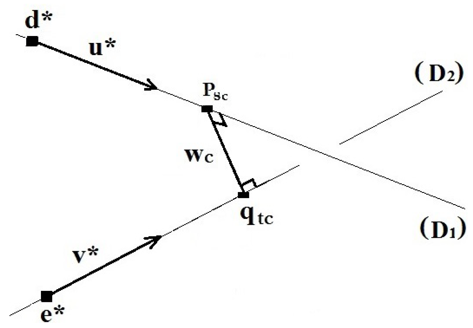
The estimation of the minimum distance between two lines in the considered L-dimensional space is achieved by finding two points, respectively, ${\mathbf{p}}_{s_C}$ on one of the lines (denoted $D_1$) and ${\mathbf{q}}_{t_C}$ on the other line (denoted $D_2$), where this minimum occurs [16]. $D_1$ and $D_2$ are, respectively, defined by the following parametric equations,

$${\mathbf{p}}_s=s{\mathbf{u}}^{*}+{\mathbf{d}}^{*}\mathrm{and}{\mathbf{q}}_t=t{\mathbf{v}}^{*}+{\mathbf{e}}^{*}.$$

(33)

$\mathbf{w}(s,t)={\mathbf{p}}_s-{\mathbf{q}}_t$ is the vector defined by two arbitrary points on the two lines. Our goal is to find w($s_C,t_C$) (hereafter denoted w${}_C$) that has the minimum length among all the s and t. To this end, we have to find the line segment (${\mathbf{p}}_{s_C}{\mathbf{q}}_{t_C}$) joining these points and which is simultaneously perpendicular to the two lines $D_1$ and $D_2$ [16], as shown in Figure 3.

In other words, the vector w${}_C$ is perpendicular to the direction vectors ${\mathbf{u}}^{*}$ and ${\mathbf{v}}^{*}$, and this is equivalent to meeting the two conditions ${\mathbf{u}}^{*T}{\mathbf{w}}_C=0$ and ${\mathbf{v}}^{*T}{\mathbf{w}}_C=0$.

We can easily solve this couple of equations by replacing w${}_C$ by (${\mathbf{p}}_{s_C}-{\mathbf{q}}_{t_C}$) and using (33). Denoting ${\mathbf{w}}_0={\mathbf{d}}^{*}-{\mathbf{e}}^{*}$, this yields

$$\begin{array}{ccc}\hfill ({\mathbf{u}}^{*T}{\mathbf{u}}^{*})s_C-({\mathbf{u}}^{*T}{\mathbf{v}}^{*})t_C& =& -{\mathbf{u}}^{*T}{\mathbf{w}}_0\hfill \\ \hfill ({\mathbf{v}}^{*T}{\mathbf{u}}^{*})s_C-({\mathbf{v}}^{*T}{\mathbf{v}}^{*})t_C& =& -{\mathbf{v}}^{*T}{\mathbf{w}}_0.\hfill \end{array}$$

Then, by denoting $a_1={\mathbf{u}}^{*T}{\mathbf{u}}^{*}$, $a_2={\mathbf{u}}^{*T}{\mathbf{v}}^{*}$, $a_3={\mathbf{v}}^{*T}{\mathbf{v}}^{*}$, $a_4={\mathbf{u}}^{*T}{\mathbf{w}}_0$, and $a_5={\mathbf{v}}^{*T}{\mathbf{w}}_0$, we obtain

$$s_C=\frac{a_3{a}_4-a_5{a}_2}{{a_2}^2-a_1{a}_3},t_C=\frac{a_2{a}_4-a_1{a}_5}{{a_2}^2-a_1{a}_3},\mathrm{with}{a_2}^2-a_1{a}_3\ne 0.$$

From Equation (33), by replacing s and t by $s_C$ and $t_C$, we can thus estimate the points $p_{s_C}$ and $q_{t_C}$ on the two lines $D_1$ and $D_2$, where they are the closest to each other.

In practice, if the minimum distance between the two lines, denoted

$$d(D_1,D_2)=∥{\mathbf{p}}_{s_C}-{\mathbf{q}}_{t_C}∥,$$

(34)

is less than a threshold, the mean of the coordinates of ${\mathbf{p}}_{s_C}$ and ${\mathbf{q}}_{t_C}$ is retained as being the point of intersection of these lines, and therefore one of the columns of the sought mixing matrix R. Otherwise, we conclude that the considered two lines do not share a common source. This is repeated for all the other pairs of lines.

Taking advantage of the above analysis, one may instead estimate the minimum-distance points of two lines by using the least squares method. Indeed, considering the parametric equations of the lines (33), we can proceed as follows,

$$\begin{array}{ccc}\hfill {\mathbf{p}}_s-{\mathbf{q}}_t& =& (s{\mathbf{u}}^{*}-t{\mathbf{v}}^{*})-{\mathbf{e}}^{*}+{\mathbf{d}}^{*}\hfill \end{array}$$

(35)

$$\begin{array}{ccc}& =& \left[{\mathbf{u}}^{*}-{\mathbf{v}}^{*}\right]\left[\begin{array}{c}s\\ t\end{array}\right]-{\mathbf{e}}^{*}+{\mathbf{d}}^{*}.\hfill \end{array}$$

(36)

By using the following notations,

$$\begin{array}{ccc}\hfill \left[\begin{array}{c}s\\ t\end{array}\right]& =& \mathbf{y}\hfill \\ \hfill \left[{\mathbf{u}}^{*}-{\mathbf{v}}^{*}\right]& =& A\hfill \\ \hfill {\mathbf{e}}^{*}-{\mathbf{d}}^{*}& =& \mathbf{b},\hfill \end{array}$$

(37)

we seek to estimate ${\mathbf{y}}^{*}$ such that

$${\mathbf{y}}^{*}=\underset{y}{argmin}∥A\mathbf{y}-\mathbf{b}∥.$$

We can solve this problem by applying the least squares method, whose solution is (for a full-column-rank matrix A):

$${\mathbf{y}}^{*}={\left(A^{T}A\right)}^{-1}{A}^T\mathbf{b}.$$

As in the first method detailed above, if the minimum distance between the two lines is less than a threshold, the mean of the coordinates of ${\mathbf{p}}_{s_C}$ and ${\mathbf{q}}_{t_C}$, obtained from Equation (33), is retained as being one of the columns of the sought mixing matrix. The above least squares method was used in the simulations reported in Section 6.

4.3. Extraction Step (Step 3)

After estimating the spectrum of each pure material, the last step of the proposed approach consists in extracting the M abundance maps (sources) that are present in the considered data. To this end, we apply a least squares method with non-negativity constraint (“Non-negative Least Squares” (NLS)) [17] to each pixel of the considered image. This is achieved as follows,

$$\begin{array}{ccc}\hfill \widehat{\mathbf{f}}\left(n\right)& =& \underset{\mathbf{f}\left(n\right)}{argmin}∥R\mathbf{f}\left(n\right)-\mathbf{x}\left(n\right)∥\forall n\in \left\{1\cdots N\right\}\hfill \\ & & \mathrm{subject}\mathrm{to}\mathbf{f}\left(n\right)\ge 0.\hfill \end{array}$$

(38)

This method requires the number of non-zero elements in the estimated vector $\widehat{\mathbf{f}}\left(n\right)$ to be at most equal to the number of elements in the vector $\mathbf{x}\left(n\right)$. This is verified thanks to Assumption 5. Furthermore, to handle the imposed sum-to-one constraints (10), we add a row consisting of the same positive constant value to the mixing matrix R and to the observation matrix X [18].

It should be noted that the above first two steps of BiS-Corr are directly applicable to multispectral and hyperspectral images (whereas the above-mentioned constraint in the third step of BiS-Corr may not be met for images which have a very low number of bands). Moreover, tests performed with simulated data especially showed for hyperspectral images that the number of two-source zones detected in Step 1 was lower when adding white noise to the images, with a signal to noise ratio varying between 60 and 40 dB, as compared with the number of zones detected with the noise-free version of the same image (for the same threshold value in the detection criterion). This reduction of the number of detected zones then led to the reduction of the number of associated identified lines, which are necessary for the next stages of the proposed approach (Parts 2 and 3 of Step 2). This problem was solved by adding a preliminary step into the BiS-Corr method, before the above-defined Step 1. This preliminary step achieves dimensionality reduction by performing Principal Component Analysis (PCA): it creates K new spectral bands, equal to the K first components of the considered data, here with $K=M$ where M is the number of sources selected for the performed simulations. This preliminary step not only decreases the complexity of the endmember spectra extraction but also reduces the noise possibly contained in the considered data [1]. The proposed BiS-Corr method thus first extracts the representation of the unmixed data in the PCA-based K-dimensional subspace, ideally without loss of information, as the noise-free original data are in that subspace. Then, using the full-dimensional (dimension equal to L) inverse PCA basis-to-basis transform, the unmixed spectra are finally transformed back to the original data representation space, so as to extract the L-component pure material spectra.

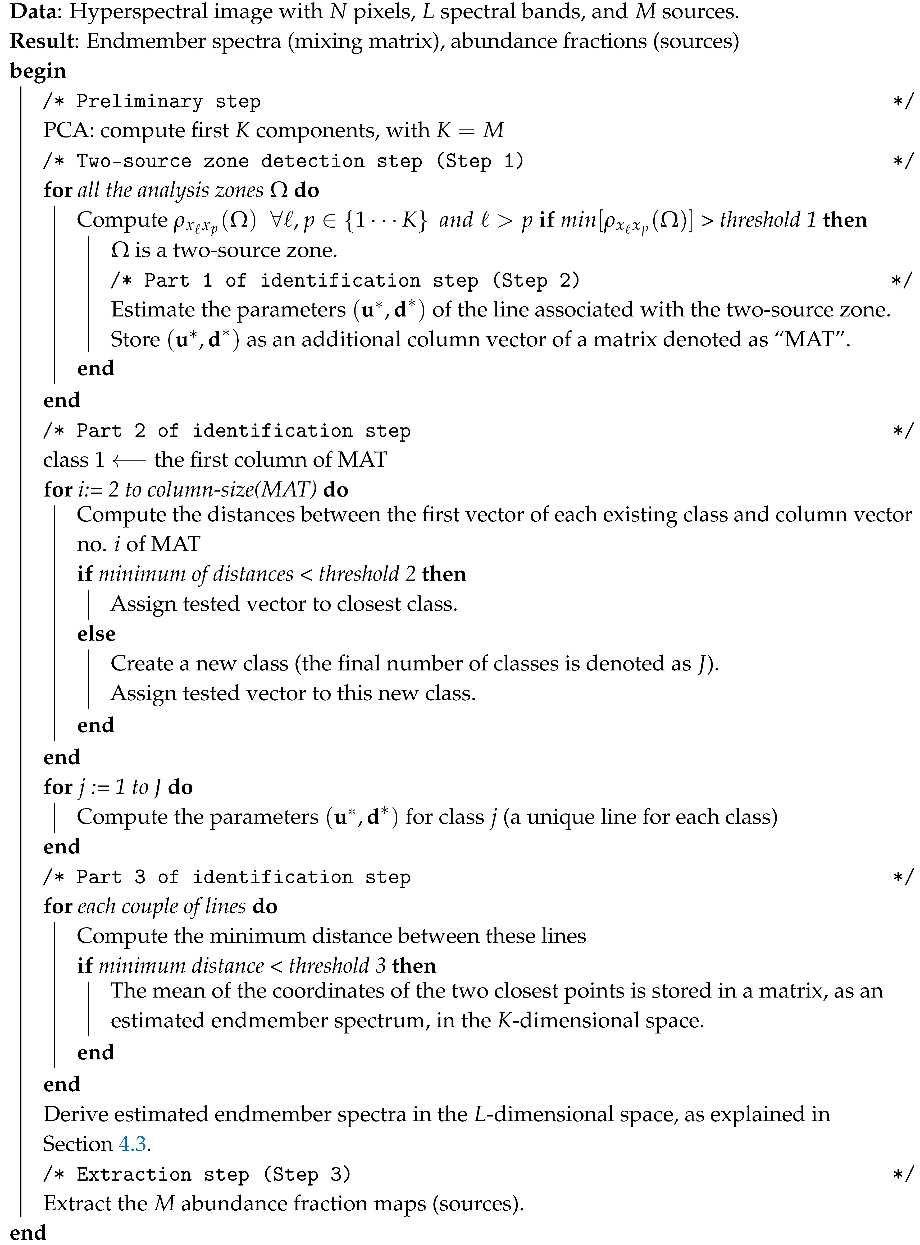
The pseudo-code of the BiS-Corr method is provided in Algorithm 1.

Algorithm 1: BiS-Corr method.

5. Materials

In this section, we present a few details on the hyperspectral images which were used in our tests and were created by numerically combining real pure material spectra and synthetic but realistic abundance maps. The latter are detailed hereafter.

5.1. Data Used in Test 1

The image used in the first experiment was obtained as follows.

• Create 3 abundance fraction maps, each of them containing 50 × 50 samples obtained using a Dirichlet distribution, which is known to be a relevant model for abundance fractions. More specifically, the used maps were created so as to keep only the pixels with abundance fractions lower than 0.8 (only significantly mixed pixels, to address complex configurations). For more details about the obtained abundance fractions, the reader may refer to [19,20], especially to the spectMixGen Matlab function.
• Modify the above maps by creating 3 two-source zones, each containing 5 × 5 samples, with a common source for each pair of zones. For the first zone: presence of sources 1 and 2, for the second zone: presence of sources 1 and 3, and finally for the third zone: presence of sources 2 and 3.
• Mix these 3 abundance maps using the linear model (1) with a mixing matrix composed of 3 pure material spectra (with 420 wavelengths). These spectra were arbitrarily chosen from the USGS spectral library [21].
• Corrupt the image with additive white noise, with a 40-dB Signal-to-Noise Ratio (SNR).

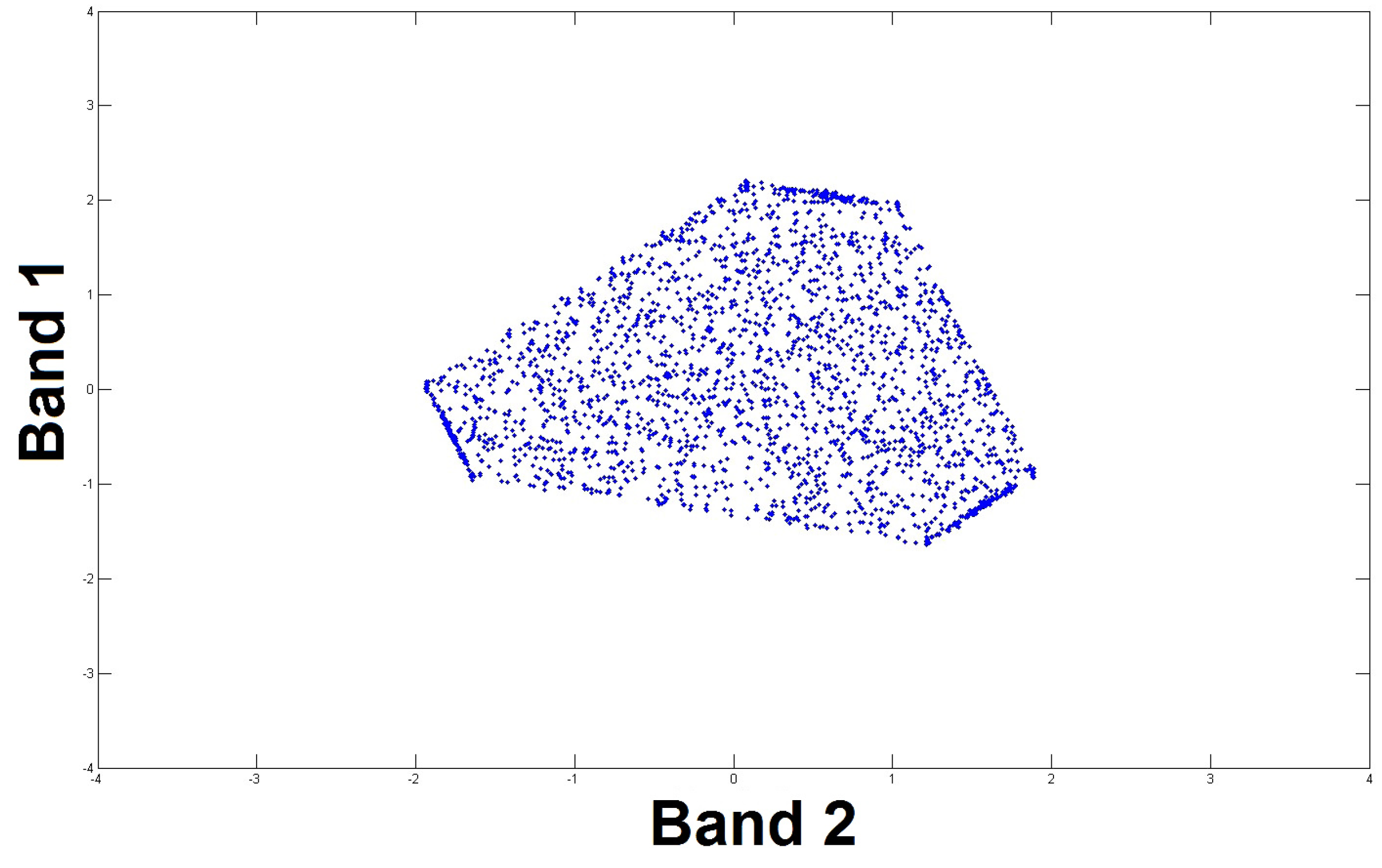
A 2D scatter plot derived from this image is shown in Figure 4.

5.2. Data Used in Test 2

The image used hereafter was obtained as follows.

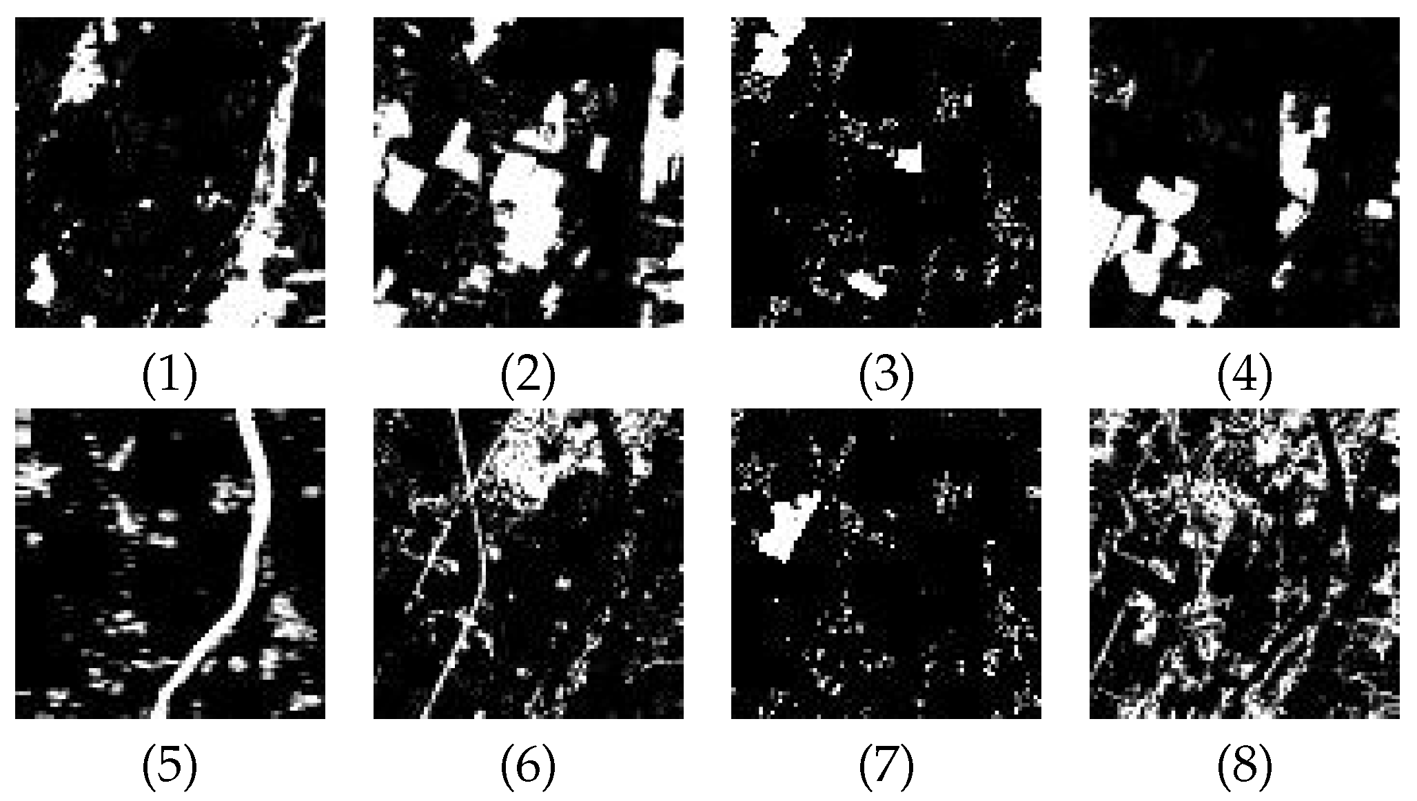
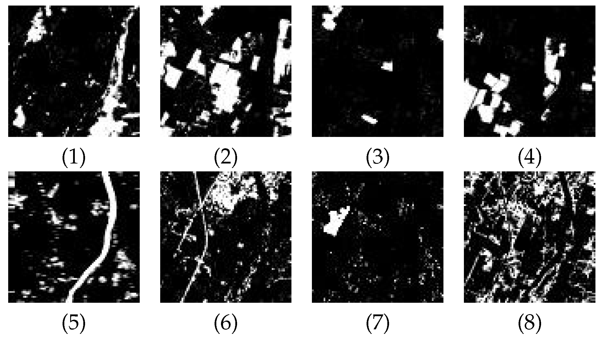
• Create 8 realistic abundance fraction maps consisting of 80 × 80 pixels. These maps were derived from a real classification (see in [12] for details), by averaging pixel classification values on sliding $5\times 5$ windows. The obtained sources are shown in Figure 5.
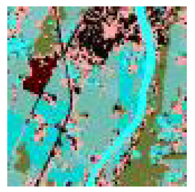
• Derive a hyperspectral image by linearly combining the above sources with a mixing matrix containing eight 224-band spectra. The used spectra were randomly chosen from the USGS spectral library [21]. The RGB (Red, Green, Blue) composition of the “observations” thus obtained is shown in Figure 6.
• Corrupt the image with additive white noise, with a 45-dB SNR.

6. Experimental Results

In this section, we present results obtained by applying the proposed BiS-Corr method and various BSS methods from the literature. We first define the performance criteria used to evaluate the quality of the results, and then we show the results of experiments.

6.1. Performance Criteria

To perform the quantitative evaluation of the test results, we used, after correction of permutations, the following two performance criteria.

• For abundance fractions: The Normalized Mean Square Error (NMSE) for the mth pure material is defined as

  $$NMS{E}_m=\frac{{∥{\mathbf{f}}_m-\widehat{{\mathbf{f}}_m}∥}^2}{{∥{\mathbf{f}}_m∥}^2},$$

  (39)

  where the vector ${\mathbf{f}}_m$ contains the actual abundance fractions used in all pixels of the simulated image for the mth pure material, and $\widehat{{\mathbf{f}}_m}$ is its estimate provided by the considered BSS method.
• For reflectance spectra: The spectral angle mapper (SAM) for the mth pure material is defined as

  $$SA{M}_m=arccos(\frac{〈{\mathbf{r}}_m,\widehat{{\mathbf{r}}_m}〉}{∥{\mathbf{r}}_m∥·∥\widehat{{\mathbf{r}}_m}∥}),$$

  (40)

  where $\widehat{{\mathbf{r}}_m}$ is the considered estimate of ${\mathbf{r}}_m$.

In most cases, the comparison of BSS methods is hereafter performed on the basis of average values of SAM and NMSE obtained over all M pure materials.

6.2. Results

6.2.1. Test 1

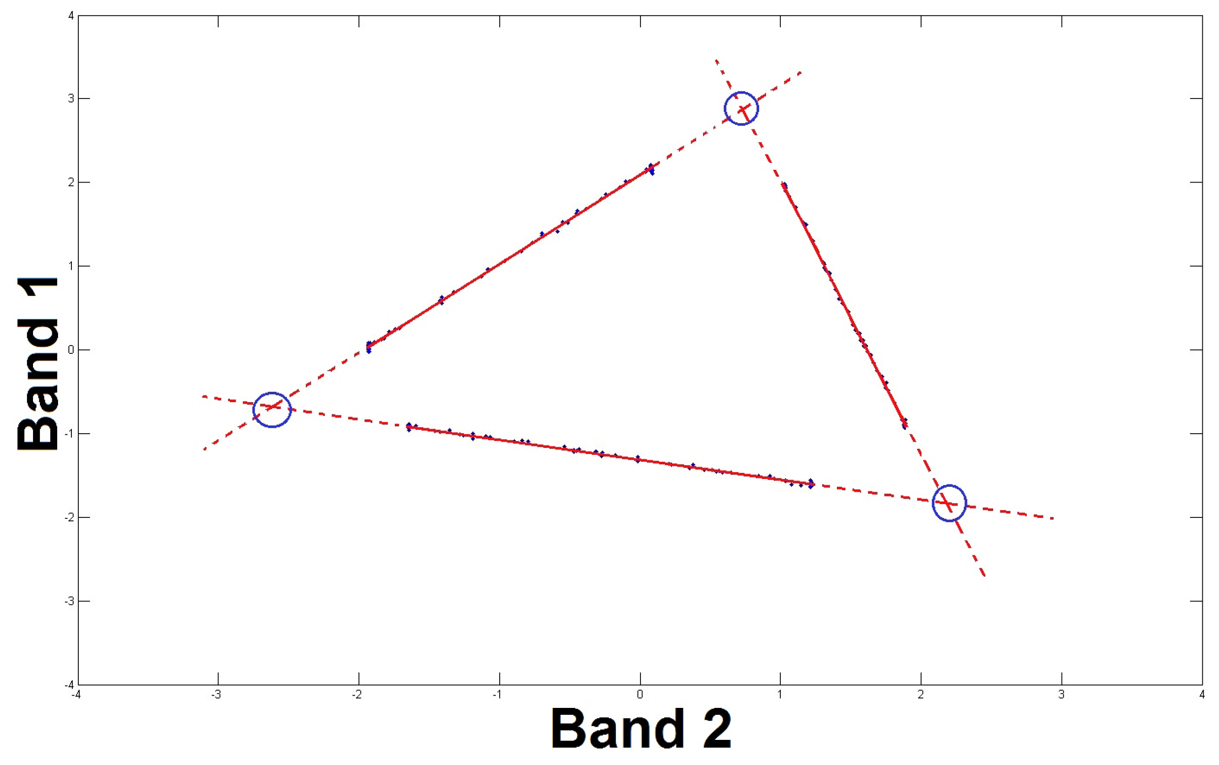
As explained in Section 4, after detecting all two-source zones of the considered image, and after estimating and classifying the parameters generated by these zones (Parts 1 and 2 of Step 2), we get the different lines shown in Figure 7. As detailed in Section 3, the lines associated with all detected zones of this experiment concern the case that is the most difficult to solve, when the points corresponding to each pair of sources do not include the bounds of the possible segments. The latter bounds correspond to pure pixels and are illustrated by the three small circles in Figure 7.

Therefore, and under the assumption of the existence of a common point between the two lines composing each pair of lines, the coordinates of each pure material spectrum are precisely estimated by calculating the point of intersection of each pair of lines (Part 3 of Step 2). These intersection points are illustrated by the small circles in Figure 7.

The geometrical unmixing methods from the literature used for comparison in this experiment are as follows. The methods based on the assumption of the presence of pure pixels are Vertex Component Analysis (VCA) [22], Orthogonal Subspace Projection (OSP) [23], and N-FINDR [24]. The methods based on minimizing the volume of the simplex formed by the data are Minimum Volume Simplex Analysis (MVSA) [25] and Simplex Identification via Split Augmented Lagrangian (SISAL) [20]. All these methods only provide estimates of the pure material spectra. Therefore,

Table 1. Spectral angle mapper (SAM) (in degrees) of estimated spectra, using BiS-Corr, Vertex Component Analysis (VCA), Orthogonal Subspace Projection (OSP), N-FINDR, Minimum Volume Simplex Analysis (MVSA), and Simplex Identification via Split Augmented Lagrangian (SISAL).

	Material No. 1	Material No. 2	Material No. 3	Mean Over All Materials
$\mathbf{BiS}-\mathbf{Corr}$	$0.04$	$0.09$	$0.06$	$0.05$
$\mathbf{VCA}$	$1.07$	$3.48$	$1.86$	$1.60$
$\mathbf{OSP}$	$1.21$	$10.01$	$3.97$	$3.79$
$\mathbf{N}-\mathbf{FINDR}$	$6.78$	$3.64$	$1.88$	$3.08$
$\mathbf{MVSA}$	$0.04$	$0.18$	$0.08$	$0.08$
$\mathbf{SISAL}$	$0.03$	$0.19$	$0.06$	$0.07$

only contains the above-defined spectral performance criterion (the SAM) of the classical and proposed methods.

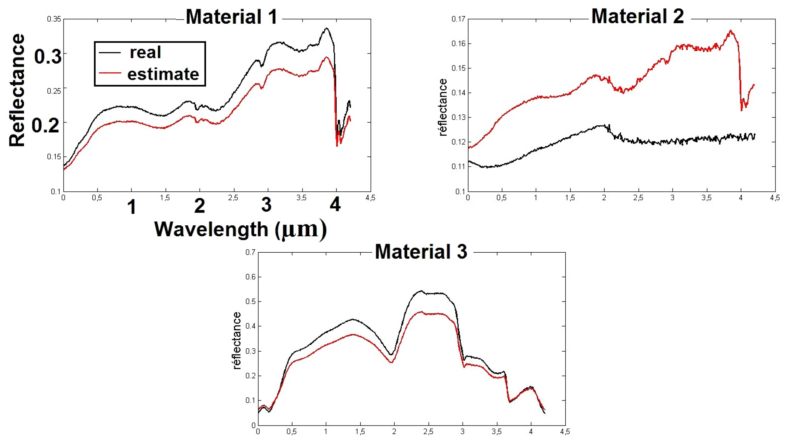
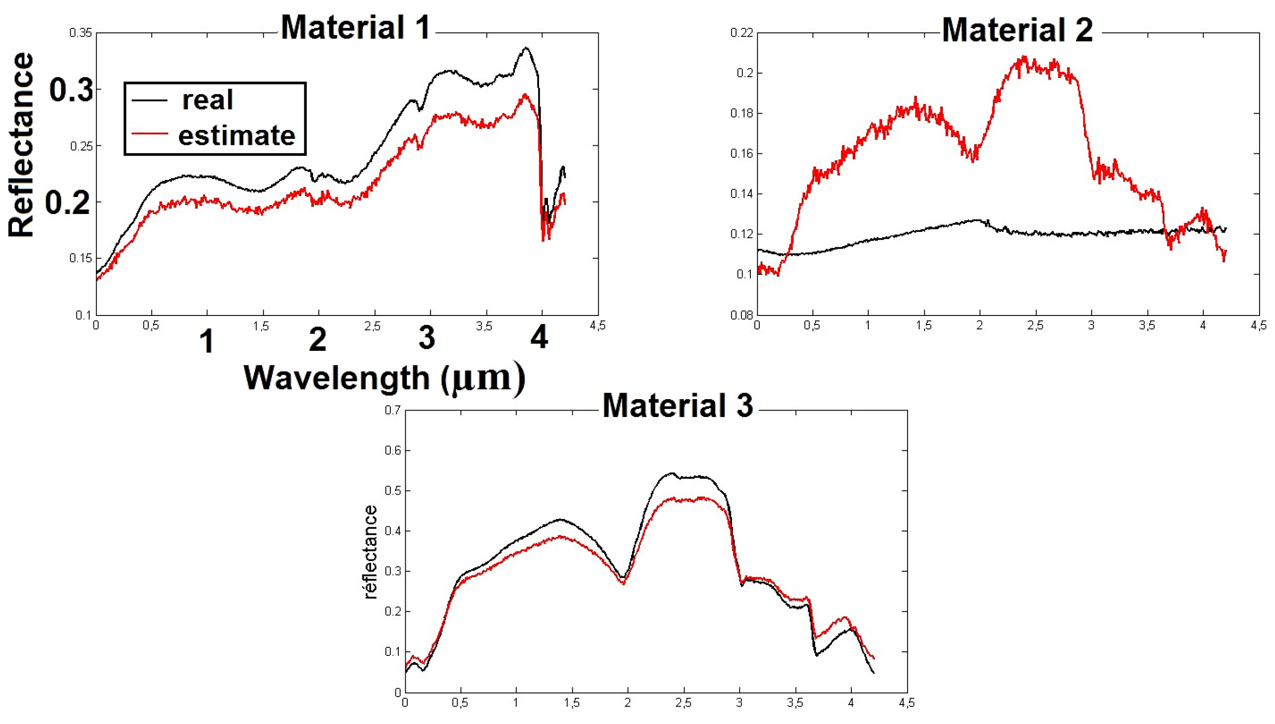
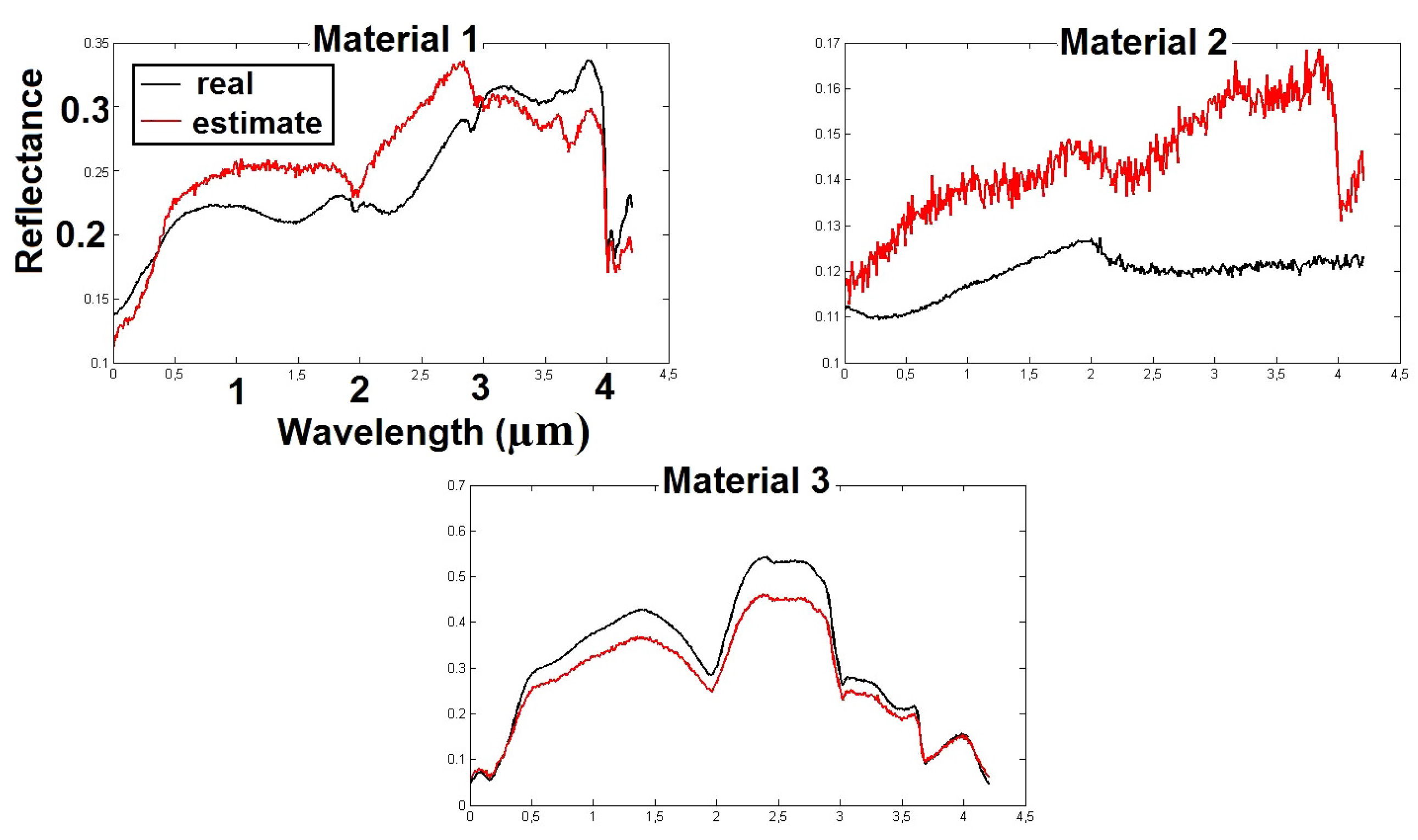
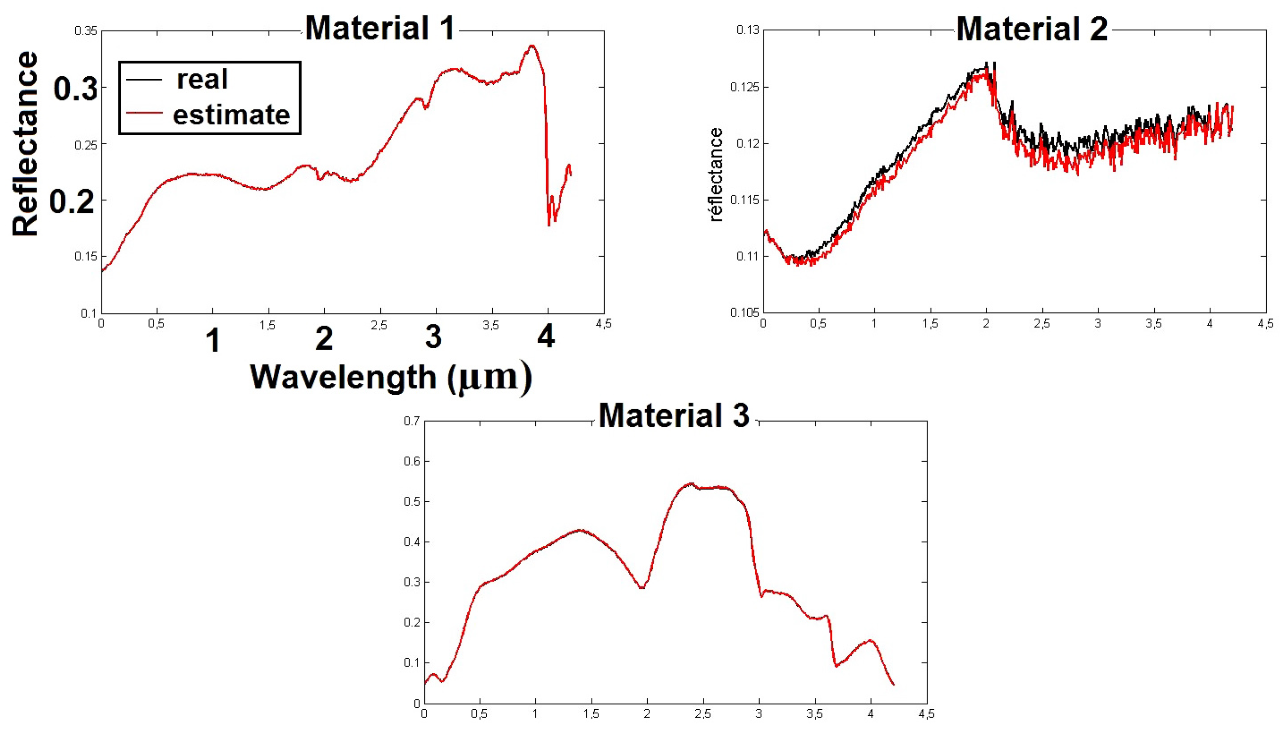
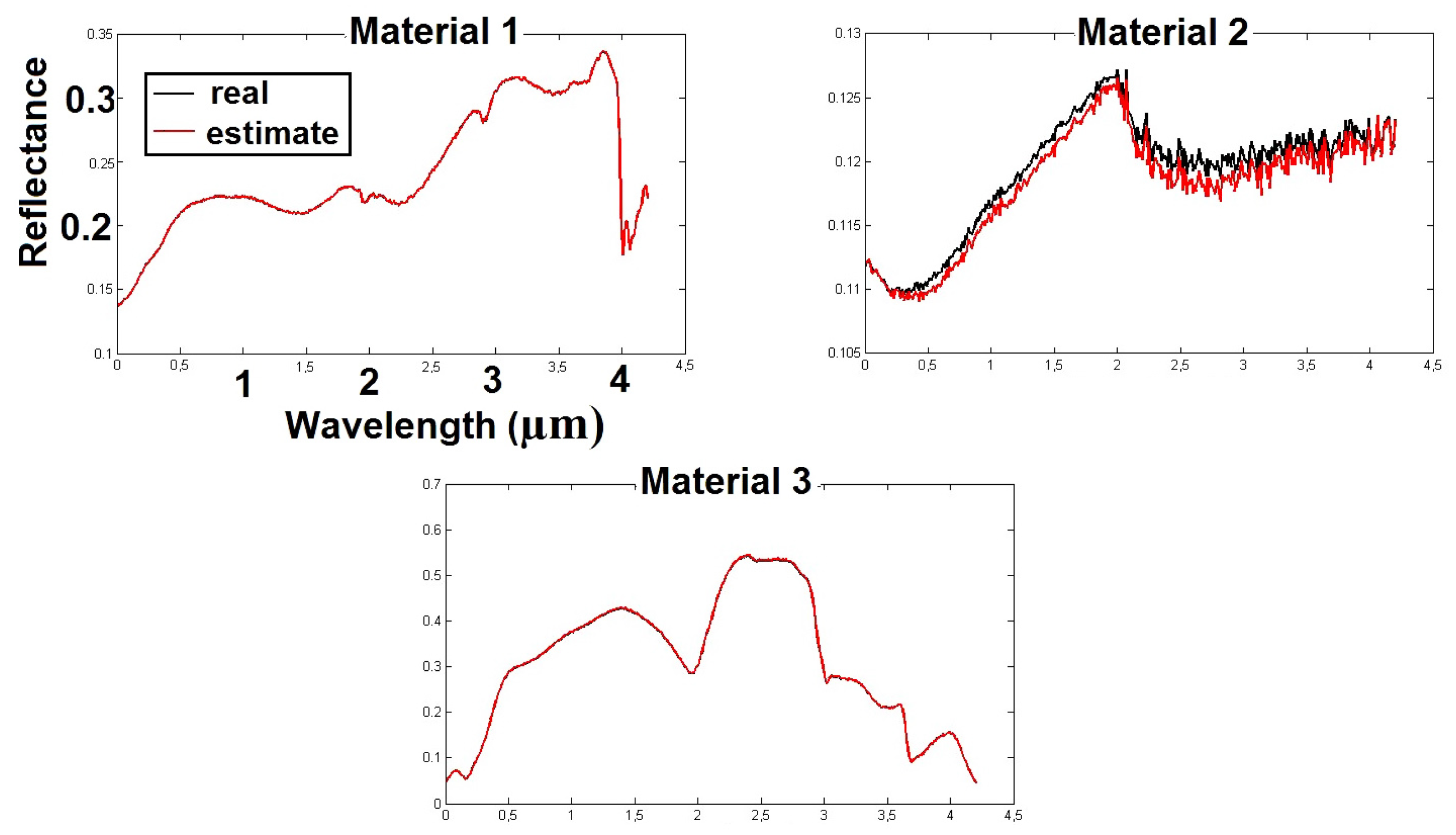
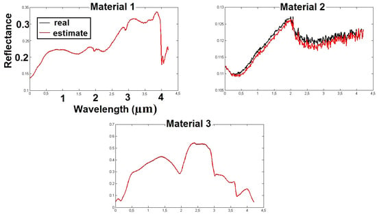
The superposition of the pure material spectra used in this test and of their estimates is given in Figure 8, Figure 9, Figure 10, Figure 11, Figure 12 and Figure 13.

6.2.2. Test 2

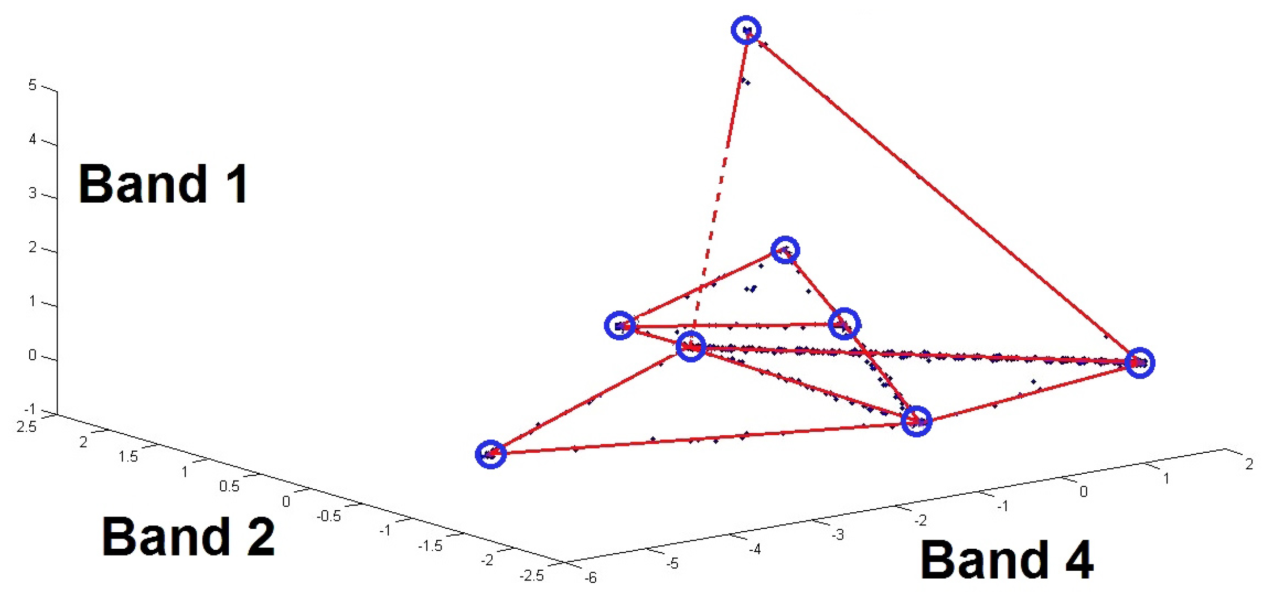
The two-source lines provided by the BiS-Corr method for this image are shown in Figure 14. As in the previous test, the coordinates of each endmember spectrum are precisely estimated by calculating the point of intersection of each pair of lines. These intersection points are illustrated by the small circles in Figure 14. For readability reasons, we have chosen to present the spectral bands 1, 2, and 4.

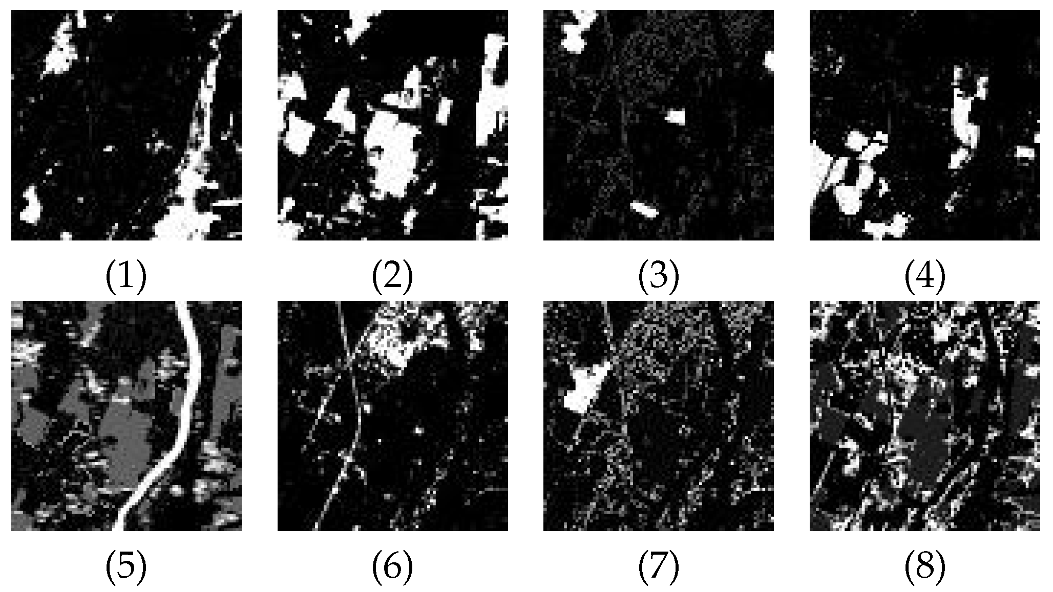
Figure 15 shows the superposition of one of the pure spectra used in this test and of its estimate, which perfectly fits the shape of the actual pure spectrum. The estimated abundance fraction maps are provided in Figure 16. They are similar to the actual maps, shown in Figure 5.

We then compare the numerical performance of BiS-Corr and of two types of methods from the literature. The first type consists of methods that simultaneously estimate the mixing matrix and the sources, namely, SMACC [26] (available in a commercial image processing software) and MVC-NMF [27]. For MVC-NMF, we used 10 different random initializations and we hereafter present the average of the 10 results thus obtained. The methods belonging to the second type only estimate the mixing matrix. Among them, we hereafter again use MVSA, SISAL, and VCA.

The results of this experiment are detailed in

Table 2. SAM (in degrees) and NMSE obtained with: (a) BiS-Corr, (b) SMACC, and (c) MVC-NMF for each of the eight pure materials, and mean over them.

		Mat. (1)	Mat. (2)	Mat. (3)	Mat. (4)	Mat. (5)	Mat. (6)	Mat. (7)	Mat. (8)	Mean
$\mathbf{A}$	SAM	$0.04$	$0.02$	$0.08$	$0.01$	$0.01$	$0.29$	$0.21$	$0.02$	$0.07$
	NMSE	$0.002$	$0.003$	$0.020$	$0.004$	$0.003$	$0.007$	$0.008$	$0.003$	$0.006$
$\mathbf{B}$	SAM	$0.39$	$8.87$	$0.33$	$0.34$	$0.25$	$0.58$	$0.74$	$0.28$	$1.31$
	NMSE	$0.025$	$0.260$	$0.120$	$0.099$	$0.430$	$0.048$	$0.205$	$0.045$	$0.137$
$\mathbf{C}$	SAM	$10.31$	$14.20$	$12.66$	$13.67$	$12.79$	$15.69$	$10.99$	$10.17$	$12.5$
	NMSE	$0.405$	$0.527$	$0.421$	$0.472$	$0.432$	$0.338$	$1.934$	$0.323$	$0.606$

and

Table 3. SAM (in degrees) obtained with: (A) BiS-Corr, (B) VCA, (C) SISAL, and (D) MVSA for each of the eight pure materials, and mean over them.

	Mat. (1)	Mat. (2)	Mat. (3)	Mat. (4)	Mat. (5)	Mat. (6)	Mat. (7)	Mat. (8)	Mean
$\mathbf{A}$	$0.04$	$0.02$	$0.08$	$0.01$	$0.01$	$0.29$	$0.21$	$0.02$	$0.07$
$\mathbf{B}$	$0.10$	$0.09$	$0.07$	$0.08$	$0.07$	$0.14$	$0.17$	$0.06$	$0.09$
$\mathbf{C}$	$1.67$	$2.31$	$0.52$	$0.73$	$0.38$	$1.15$	$3.95$	$1.85$	$1.39$
$\mathbf{D}$	$1.42$	$0.40$	$0.64$	$0.40$	$0.44$	$2.73$	$4.90$	$0.92$	$1.32$

, and in the Figure 17 and Figure 18.

7. Discussion

7.1. Test 1

The above table and figures presented in the previous section (Test 1 results) show that the proposed BiS-Corr method succeeds in estimating the sought spectra with very high accuracy, despite the absence of pure pixels and the presence of additive noise. As expected, the three tested methods which require pure pixels here yield much lower performance. As also anticipated, the MVSA and SISAL methods, which do not require pure pixels, yield relatively similar performance levels as compared to BiS-Corr. However, the above numerical results and shapes of actual and estimated spectra show that the BiS-Corr method globally yields very encouraging results as compared with other tested methods. In particular, only BiS-Corr provides a SAM lower than $0.1$ degree for all estimated spectra.

7.2. Test 2

The proposed BiS-Corr method here again yields better performances than the other tested methods.

In particular, Table 2 shows that only the SMACC and MVC-NMF methods completely fail to obtain some sources, for example, sources 5 and 7 concerning SMACC, which is known in particular because of its availability in a commercial image processing software. All the maps estimated by the SMACC method are given as an example, in Figure 17. This figure confirms that SMACC poorly estimates sources 5 and 7, unlike BiS-Corr, due to the presence in the considered image of two-source zones covering all the sought sources.

Moreover, Table 3 shows that BiS-Corr outperforms VCA, SISAL, and MVSA, with an average SAM of approximately $0.07$ degrees. Among the latter methods, only VCA yields almost the same mean performance as BiS-Corr. This results from fact that the image considered here contains pure pixels (unlike in Test 1), which are exploited by VCA (whereas BiS-Corr is more attractive in the sense that it does not require such pure pixels). The performance of the other classical methods considered in Table 3 is illustrated in Figure 18: these methods yield limited accuracy, so that their estimated spectra are not superimposed with the actual one, whereas the estimated spectrum provided by BiS-Corr perfectly fits the actual one.

Globally, the results presented in this section for the proposed BiS-Corr method are therefore very encouraging and better than those obtained with the tested methods from the literature, for most of the considered materials.

8. Conclusions

In this paper, we proposed a new unsupervised unmixing approach called BiS-Corr, based on spatial sparsity and especially applicable to hyperspectral images. This approach consists of three steps (after dimensionality reduction):

• Determination of all the two-source zones present in the considered data, using a correlation-based detector.
• Identification of the columns of the mixing matrix (reflectance spectra of pure materials) from the intersections of the lines associated with the two-source zones.
• Reconstruction of the searched sources (abundance fraction maps) using a non-negative least squares method.

We experimentally validated the effectiveness of the proposed BiS-Corr method, with hyperspectral images obtained by numerically combining actual pure material spectra and realistic abundance maps. Moreover, the detailed tests reported above show that BiS-Corr yields better overall performance than all tested methods from the literature. Beyond that investigation, other unmixing methods related to BiS-Corr might be introduced, e.g., by developing other criteria for detecting two- or three-source zones. Other classification methods for parameters associated with such zones of interest will also be explored.

References

1. Bioucas-Dias, J.M.; Plaza, A.; Dobigeon, N.; Parente, M.; Du, Q.; Gader, P.; Chanussot, J. Hyperspectral unmixing overview: Geometrical, statistical, and sparse regression-based approaches. IEEE J. Sel. Top. Appl. Earth Obs. Remote Sens. 2012, 5, 354–379. [Google Scholar] [CrossRef] [Green Version]
2. Plaza, J.; Hendrix, E.M.T.; Garcia, I.; Martin, G.; Plaza, A. On endmember identification in hyperspectral images without pure pixels: A comparison of algorithms. J. Math. Imaging Vis. 2012, 42, 163–175. [Google Scholar] [CrossRef]
3. Dobigeon, N.; Tourneret, J.-Y.; Richard, C.; Bermudez, J.C.M.; McLaughlin, S.; Hero, A.O. Nonlinear unmixing of hyperspectral images: Models and algorithms. IEEE Signal Process. Mag. 2014, 31, 82–94. [Google Scholar] [CrossRef] [Green Version]
4. Ma, W.-K.; Bioucas-Dias, J.M.; Chan, T.-H.; Gillis, N.; Gader, P.; Plaza, A.J.; Ambikapathi, A.; Chi, C.-Y. A signal processing perspective on hyperspectral unmixing: Insights from remote sensing. IEEE Signal Process. Mag. 2014, 31, 67–81. [Google Scholar] [CrossRef] [Green Version]
5. Jourjine, A.; Rickard, S.; Yilmaz, O. Blind separation of disjoint orthogonal signals: Demixing N sources from 2 mixtures. IEEE Int. Conf. Acoust. Speech Signal Process. 2000, 5, 2985–2988. [Google Scholar]
6. Yilmaz, O.; Rickard, S. Blind separation of speech mixtures via time-frequency masking. IEEE Trans. Signal Process. 2004, 52, 1830–1847. [Google Scholar] [CrossRef]
7. Georgiev, P.; Theis, F.; Cichocki, A. Sparse component analysis and blind source separation of underdetermined mixtures. IEEE Trans. Neural Netw. 2005, 16, 992–996. [Google Scholar] [CrossRef] [PubMed]
8. Li, Y.; Amari, S.-I.; Cichocki, A.; Ho, D.W.C.; Xie, S. Underdetermined blind source separation based on Sparse representation. IEEE Trans. Signal Process. 2006, 54, 423–437. [Google Scholar]
9. Deville, Y.; Puigt, M. Temporal and time-frequency correlation-based blind source separation methods. Part I: Determined and underdetermined linear instantaneous mixtures. Signal Process. 2007, 87, 374–407. [Google Scholar] [CrossRef] [Green Version]
10. Abrard, F.; Deville, Y. A time-frequency blind signal separation method applicable to underdetermined mixtures of dependent sources. Signal Process. 2005, 85, 1389–1403. [Google Scholar] [CrossRef]
11. Deville, Y.; Bissessur, D.; Puigt, M.; Hosseini, S.; Carfantan, H. A time-scale correlation-based blind separation method applicable to correlated sources. Eur. Symp. Artif. Neural Netw. 2006, 337–343. [Google Scholar]
12. Karoui, M.S.; Deville, Y.; Hosseini, S.; Ouamri, A. Blind spatial unmixing of multispectral images: New methods combining sparse component analysis, clustering and non-negativity constraints. Pattern Recognit. 2012, 45, 4263–4278. [Google Scholar] [CrossRef]
13. Keshava, N.; Mustard, J.F. Spectral Unmixing. IEEE Signal Process. Mag. 2002, 19, 44–57. [Google Scholar] [CrossRef]
14. Wold, S. Principal component analysis. Chemometr. Intell. Lab. Syst. 1987, 2, 37–52. [Google Scholar] [CrossRef]
15. Smilde, A.; Bro, R.; Geladi, P. Multi-Way Analysis with Applications in the Chemical Sciences; John Wiley and Sons: Hoboken, NJ, USA, 2004. [Google Scholar]
16. Schneider, P.J.; Eberly, D.H. Geometric Tools for Computer Graphics; Elsevier Science: Amsterdam, The Netherlands, 2003. [Google Scholar]
17. Lawson, C.L.; Hanson, R.J. Solving Least Squares Problems; Society for Industrial and Applied Mathematics: Philadelphia, PA, USA, 1995. [Google Scholar]
18. Heinz, D.C.; Chang, C.-I. Fully constrained least squares linear spectral mixture analysis method for material quantification in hyperspectral imagery. IEEE Trans. Geosci. Remote Sens. 2001, 39, 529–545. [Google Scholar] [CrossRef] [Green Version]
19. Bioucas-Dias, J.M. Available online: http://www.lx.it.pt/~bioucas/code.htm (accessed on 20 July 2020).
20. Bioucas-Dias, J.M. A variable splitting augmented Lagrangian approach to linear spectral unmixing. In Proceedings of the IEEE Workshop on Hyperspectral Image and Signal Processing Evolution in Remote Sensing, Grenoble, France, 26–28 August 2009. [Google Scholar]
21. Clark, R.N.; Swayze, G.A.; Wise, R.; Livo, E.; Hoefen, T.; Kokaly, R.; Sutley, S.J. USGS Digital Spectral Library splib06a. U.S. Geological Survey. Digital Data Series 231. 2007. Available online: http://speclab.cr.usgs.gov/spectral.lib06 (accessed on 20 July 2020).
22. Nascimento, J.M.P.; Bioucas-Dias, J.M. Vertex component analysis: A fast algorithm to unmix hyperspectral data. IEEE Trans. Geosci. Remote Sens. 2005, 43, 898–910. [Google Scholar] [CrossRef] [Green Version]
23. Harsanyi, J.C.; Chang, C.-I. Hyperspectral image classification and dimensionality reduction: An orthogonal subspace projection approach. IEEE Trans. Geosci. Remote Sens. 1994, 32, 779–785. [Google Scholar] [CrossRef] [Green Version]
24. Winter, M.E. N-FINDR: An algorithm for fast autonomous spectral end-member determination in hyperspectral data. SPIE Conf. Imaging Spectrom. V 1999, 3753, 266–275. [Google Scholar]
25. Li, J.; Bioucas-Dias, J.M. Minimum volume simplex analysis: A fast algorithm to unmix hyperspectral data. IEEE Int. Geosci. Remote Sens. Symp. 2008, 3, 250–253. [Google Scholar]
26. Gruninger, J.; Ratkowski, A.J.; Hoke, M.L. The sequential maximum angle convex cone (SMACC). In Proceedings of the Endmember Model, Algorithms for Multispectral, Hyperspectral and Ultraspectral Imagery (SPIE), Orlando, FL, USA, 12 August 2004; Volume 5425. [Google Scholar]
27. Miao, L.; Qi, H. Endmember extraction from highly mixed data using minimum volume constrained nonnegative matrix factorization. IEEE Trans. Geosci. Remote Sens. 2007, 45, 765–777. [Google Scholar] [CrossRef]
Figure 1. 2D scatter plot corresponding to two-source pixels.
Remotesensing 12 03198 g001
Figure 2. Example in 3D permitting the visualization of lines related to different pairs of sources obtained after the classification stage.
Remotesensing 12 03198 g002
Figure 3. Distance between two lines (adapted from the work in [16]).
Remotesensing 12 03198 g003
Figure 4. 2D scatter plot corresponding to spectral bands 1 and 2 provided by the dimensionality reduction step in Test 1.
Remotesensing 12 03198 g004
Figure 5. The eight sources used in Test 2 (the white color represents the values equal to one).
Remotesensing 12 03198 g005
Figure 6. RGB composition of the “observed” hyperspectral image in Test 2.
Remotesensing 12 03198 g006
Figure 7. Test 1: lines (here represented by dashed lines) associated with the two-source zones contained in the considered image (spectral bands 1 and 2 after dimensionality reduction step) and segments of these lines (here represented by solid lines) which correspond to actual data points.
Remotesensing 12 03198 g007
Figure 8. Superposition of the pure material spectra used in Test 1 and of their estimates obtained with BiS-Corr.
Remotesensing 12 03198 g008
Figure 9. Superposition of the pure material spectra used in Test 1 and of their estimates obtained with VCA.
Remotesensing 12 03198 g009
Figure 10. Superposition of the pure material spectra used in Test 1 and of their estimates obtained with OSP.
Remotesensing 12 03198 g010
Figure 11. Superposition of the pure material spectra used in Test 1 and of their estimates obtained with N-FINDR.
Remotesensing 12 03198 g011
Figure 12. Superposition of the pure material spectra used in Test 1 and of their estimates obtained with MVSA.
Remotesensing 12 03198 g012
Figure 13. Superposition of the pure material spectra used in Test 1 and of their estimates obtained with SISAL.
Remotesensing 12 03198 g013
Figure 14. Test 2: lines (in red) associated with the two-source zones contained in the used image (spectral bands 1, 2, and 4 after dimensionality reduction step).
Remotesensing 12 03198 g014
Figure 15. Superposition of one of the pure spectra and of its estimate, obtained with the proposed BiS-Corr method in Test 2.
Remotesensing 12 03198 g015
Figure 16. The eight estimated sources provided by the BiS-Corr method in Test 2.
Remotesensing 12 03198 g016
Figure 17. The eight estimated sources provided by the SMACC method in Test 2.
Remotesensing 12 03198 g017
Figure 18. One pure material spectrum used in Test 2, and its estimates obtained using the proposed approach, SISAL, and MVSA.
Remotesensing 12 03198 g018