Article

Satellite ASTER Mineral Mapping the Provenance of the Loess Used by the Ming to Build their Earthen Great Wall

1
C3DMM Pty Ltd., 3/473 Cambridge Street Floreat, Western Australia 6014, Australia
2
Key Laboratory of Digital Earth Science, Aerospace Information Research Institute, Chinese Academy of Sciences, Beijing 100094, China
3
Hengyang Base of International Centre on Space Technologies for Natural and Cultural Heritage under the Auspices of UNESCO, Hengyang 421002, China
*
Author to whom correspondence should be addressed.
Remote Sens. 2020, 12(2), 270; https://doi.org/10.3390/rs12020270
Submission received: 30 October 2019 / Revised: 7 January 2020 / Accepted: 10 January 2020 / Published: 14 January 2020
(This article belongs to the Special Issue ASTER 20th Anniversary)

Abstract

:
The earthen border wall (Great Wall) built by the Ming is largely made of wind-blown loess. However, does the composition of this loess change along the length of the wall in response to variations in regional sediment transport pathways and impacting on the wall’s erosional durability? To date, defining these sediment transport pathways has been a challenge because of the paucity of spatially-comprehensive, compositional information. Here, we show that satellite ASTER mineral maps, combined with field sample measurements along a 1200 km section of the Ming’s earthen wall, reveal both the compositional heterogeneity of loess as well as the complexity of the sediment transport pathways of individual loess components, including: (i) quartz sand from Cretaceous sandstones in the Gobi Desert; (ii) gypsum from evaporative lakes in the Tengger Desert; (iii) kaolinite from Devonian Molasse in the Qilian Shan; and (iv) chlorite and muscovite from meta-volcanic rocks exposed across the Alashan Block. Sediment transport pathways involve a combination of colluvial, aeolian and fluvial (ephemeral and permanent) processes shaped by the topography. ASTER enabled mapping of compositional gradients related to two pathways, namely: (i) quartz sand driven by aeolian saltation in concert with the Yellow River; and (ii) clay and fine silt travelling large distances (>500 km) by long-term wind suspension. The most intact section of wall is found along the Hexi Corridor, which is poor in quartz sand and rich in (kaolinitic) clay and fine-silt, driven by wind-shielding by the Alashan Block. We also found evidence that the Ming: (i) mined loess from close by the wall (<1 km); (ii) targeted loess richer in finer fractions; and (iii) routinely applied a Ca-rich additive (probably lime).

1. Introduction

The Ming Dynasty’s program of building an earthen border wall began following a decisive battle that forced the Ordos Mongols north of the Yellow River in 1473 [1]. The initial plan was to rapidly build an ~800 km border wall across the Ordos Plateau to separate sand dune-fields in the north from agriculturally productive lands in the south [2] (Figure 1a). The Ming were able to build this wall to a height of 5–8 m (Figure 1d,e) in just three months using their “hangtu” method of ramming earth between formwork [1,3]. This technique resulted in a characteristic 15–30 cm horizontal layering [4] and contrasts with that built by earlier dynasties where a thinner (7–10 cm) layering of earth was often sandwiched between horizons of rock and/or vegetation [5]. The completion of the wall across the Ordos Plateau soon delivered military success [1], giving impetus for eastward continuation towards Beijing and westward along the Hexi Corridor towards Jiayuguan (Figure 1a).
This rapid construction of the Ming’s border wall required easy access to suitable earthen building materials. Even though wind-generated loess (dominated by angular, silt-size grains) deposits are readily eroded [6,7], the Ming selected loess for wall construction because of its pervasive development at/near the surface across the Ordos Plateau, especially south of the Mu Us Desert (Figure 1a and Figure 2c). However, it is not known where the Ming mined their loess for wall construction. That is, was it sourced close by the wall (<1 km away) or from distant (>100 km), centralized, quarries?
Loess is typically buff colored, structureless, and flat-lying [8], although its thickness varies regionally. Over the Ordos Plateau, loess is up to 400 m thick [8] being the result of 20 million years of dust activity over a relatively stable platform. In contrast, loess deposits along the Hexi Corridor are much younger (Holocene) and often only 1 m thick [9]. This contrast in thickness is potentially driven by repeated uplift and erosion along the northeast margin of the Tibetan Plateau [10] and/or possibly the effects of climate-related variations in vegetation cover [9]. The most recent loess deposits include: the Late Pleistocene (11,700 to ~1,000,000 years) Malan Loess Unit, which decreases in thickness from Yinchuan (~30 m thick) to Xian (~5 m thick) (Figure 1a) [8]; and Holocene (0–11,700 years) layers, which are up to 8 m thick [11,12] and continue to accumulate today [13].
Mineral composition is a factor in the erosive potential of earthen materials. For example, minerals such as kaolinite (Al2Si2O5(OH)4) and muscovite (KAl2(AlSi3O10)(FOH)2) do not expand on wetting in contrast to montmorillonite ((Na,Ca)0.33(Al,Mg)2(Si4O10)(OH)2·nH2O) and illite ((K,H3O)(Al,Mg,Fe)2(Si,Al)4O10((OH)2,(H2O)), which swell when wet and contract when dry causing desiccation cracking and therefore are more prone to structural disintegration [14]. The cohesive strength of earthen material is also enhanced by the proportion of clay-sized material (<2 µm) because of increased levels of hydrogen bonding between water molecules and the surfaces of these grains [15], which typically comprise minerals such as kaolinite, illite, and montmorillonite. Coarser particles such as sand (63–2000 µm), which often comprises quartz (SiO2), do not share this propensity for hydrogen bonding [15,16].
Silicate minerals can also react with calcite (CaCO3), lime (Ca(OH)2), and/or quicklime (CaO) to form cementing agents such as Ca-silicates (e.g., hydrogarnets) and (recrystallized) calcite [17] as part of a “pozzolanic” reaction. Loess is an effective pozzolan as it comprises SiO2 + Al2O3 + Fe2O3 ≥ 70 wt.%. The Ming Dynasty natural scientist, Song Yingxing, described how their “tabia” or “binding material” method used lime mixed with soil and sand [18].
These considerations help explain why the rate of erosional deterioration of earthen structures at Jiaohe in northwest China is related to the mineralogy of the building materials [19]. The question is, does the composition of the loess used by the Ming change along the length of the wall? If so, then what processes are responsible for this compositional change? Finally, have changes in composition impacted on the erosional durability of the earthen wall?
In theory, dust particles with a diameter <70 μm are capable of transportation by wind suspension [20]. The <20 µm fraction (i.e., clay and fine-silt) can potentially remain in wind-suspension for several days, travelling hundreds to thousands of kilometers and is termed long-term wind suspension [20]. In contrast, the 20–70 μm fraction (i.e., coarse-silt) can remain in wind-suspension for minutes to hours, travelling distances of meters to kilometers, and is termed short-term wind suspension [20]. Grains >70 μm in size (i.e., sand) are not carried by wind-suspension but instead bounce or saltate across the land surface, travelling only meters per wind event [20]. Factors determining where this range of particle sizes can accumulate as deposits of loess include: prevailing wind direction; distance from source; and topographic and/or vegetation traps.
The large volumes of sediment required to generate the loess deposits across the Ordos Plateau and Hexi Corridor have been attributed to the combination of cold deserts juxtaposed against rapidly uplifting mountainous regions [21,22]. That is, rocks in high areas are eroded and reduced in particulate size by glacial grinding and cold weathering processes before being transported in fluvial-suspension by snowmelt-fed rivers into neighboring desert basins that act as sediment sinks to be later re-worked by wind activity. However, identifying which mountainous source areas, rivers, deserts, and/or winds were critical in loess development has proved to be much more problematic. Mountainous regions proposed as the primary source of particulate materials include: the Qilian Shan [22]; Gobi Altay [22]; Tianshan; Alashan Block; and Tibetan Plateau [23,24]. Researchers have also identified alluvial fans as a secondary source of the eroded grains, including those along the Hexi Corridor [10] and Gobi Altay Mountains [22]. Proposed sandy or stony desert secondary sources include: the Taklamakan [25]; Qaidam Basin [23]; Gobi [22,26]; Mu Us; Hobq; Ulan Buh; Tengger; and Badain Jaran [22,26,27,28,29]. Rivers include: Yellow River [25,30,31] and ephemeral rivers along the Hexi Corridor, such as the Shiyang and Heihe [32] that drain into neighboring desert basins (Figure 1a). The prevailing wind patterns alternate between westerly to northerly flows of the East Asian Winter Monsoon (EAWM) versus southerly flows of the East Asia Summer Monsoon (EASM) [26].
To date, determining the primary/secondary sources of loess material has relied on point-sample measurements of: grain size [8,33,34]; major elements [35,36]; trace elements [35]; rare earth elements [25,35]; zircon U-Pb geochronology [37,38]; scanning electron microscope energy dispersive spectrometers [27]; luminescence [39]; electron magnetic spin [40,41]; oxygen isotopes [42]; Nd and Sr isotopes [43,44]; magnetics [45]; and mineralogy [32,46,47,48,49]. However, interpreting transport pathways using such sparse point-sample data collected from heterogeneous landscapes is thwart with difficulties. Indeed, the most recent Loessfest meeting [50] concluded “there is a need to develop new methods and approaches for quantitative paleoenvironmental and paleoclimatic reconstructions”.
Geologists have been tackling a similar challenge in their targeting of economic mineral deposits by collecting spatially-comprehensive data, such as geophysical [51] and mineral mapping imagery [52], to better elucidate target fluid transport pathways that extend from source rocks to sites of potential (metal) deposition. This so-called “mineral-system” approach [53] requires both: (i) the definition of essential ingredients and their related mappable criteria; and (ii) the assembly of regional geoscientific data in order to create maps that target these mappable criteria.
Given that “the nature of the material is paramount, and the formation of the material is paramount. And this means the formation of the actual units, the actual particles [= mineral grains] which comprise the deposit of loess” [54], we propose a “loess system” based on a mappable suite of essential mineral components. The critical “loess system” mapping tool we used here for tracking the provenance of the loess sourced by the Ming to build their earthen wall is the satellite-borne, Advanced Spaceborne Thermal Emission and Reflection Radiometer (ASTER) sensor [55]. ASTER was designed to map land surface composition, albeit at moderate spectral resolution. It was launched in December 1999 and has since acquired multiple coverages of the Earth’s land surface at <83° latitude [56].
Based on the principles of mineral spectroscopy [57], we processed the calibrated ASTER imagery [58] to generate a suite of thematic mineral mapping products at ~30 m pixel resolution for an area of ~60,000 km2 spanning the 1200 km section of Ming earthen wall between Shenmu and Jiayuguan (Figure 1a). We focused here on five essential mineral components of loess, namely quartz-sand, white-mica (muscovite and illite), chlorite (as well as carbonate), gypsum and kaolinite, as these are measurable at ASTER’s spectral resolution [58,59,60,61]. Field data (optical spectra as well as other geochemical, mineralogical, and particle size measurements) from 21 sites along the Ming earthen wall were collected to provide both validation of the satellite maps as well as information about the compositional homogeneity/heterogeneity of the wall building material and any relationships with local (<100 m) surface materials.
From this multi-scale, spatially-comprehensive framework, we obtained a more detailed perspective of the compositional variability of the loess. This compositional information then provided the basis for solving the provenance of the loess used by the Ming to build their earthen wall, which has two essential parts: (i) Where did the Ming mine their loess, i.e., was it from local sources (<1 km away) or from centralized quarries many kilometers away? (ii) Where did the particles of loess originate? With regards to the second, do specific minerals partition within particle size ranges, reflecting different transport processes? In addition, has compositional heterogeneity impacted on the wall’s erosional state as this could assist in wall’s future preservation? Finally, we underline the value of using the Ming earthen wall validating our satellite ASTER mineral maps because it provides a 1200 km east–west transect across the entire study area.

2. Materials and Methods

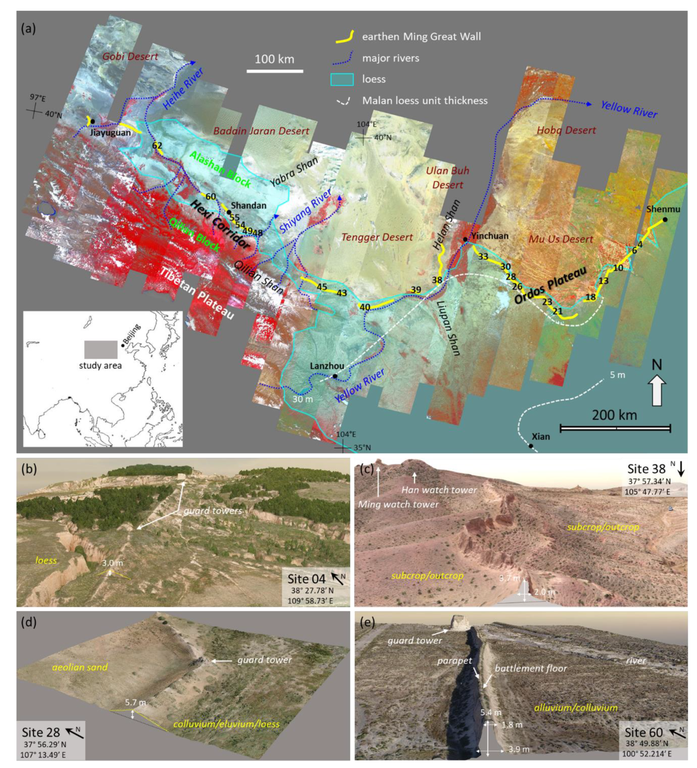
2.1. Field Recognition of the Ming Earthen Border Wall

Several features helped us establish whether a section of wall was built by the Ming or by an earlier Dynasty. The key criteria for it to be Ming related include:
  • Horizontally-layered (10–30 cm), loess-dominated building material (earlier walls are often associated with abundant rock fragments);
  • Regularly spaced guard towers (Figure 1b–e) also built using the same materials/methods;
  • Aprons of the same types of fragmented, usually glazed stoneware and porcelain containers found scattered around these guard towers; and
  • The relatively well preserved (height) nature of the earthen wall (Figure 1c), especially given that the Ming wall was the last completed in Chinese dynastic history.

2.2. Field Sampling

The Great Wall is protected by Chinese law, which is administered at the province level. Field sampling for this study thus was carefully designed to minimize any impact. Measurements types included: remote imaging, e.g., drone survey or field LIDAR; surface contact, e.g., field portable spectrometers and pXRF; and those requiring a physical sample, e.g., particle size and XRD. The field samples taken were <100 g each and were sampled as follows: (i) one sample from either side of the wall ideally from recently fallen material; (ii) surface samples 15 m to the north and south of the wall; and (iii) surface samples 45 m to the north and south of the wall. Field-portable X-ray fluorescence (pXRF) measurements were taken at each sample point. For some sites, additional samples and in situ measurements were taken, such as from within eroding layers (green arrows in Figure 2).

2.3. 3D Model Generation

A high resolution (<5 cm) 3D surface model, ortho-mosaic image, and digital elevation model (DEM) were generated for each field site (e.g., Figure 1b–e), using drone digital imagery (where allowed by government authorities) and observed at five different look angles (1 nadir and 4 oblique). Camera calibration, photo aligning, dense point-cloud building, mesh and texture building, DEM, and ortho-mosaic building were processed with photogrammetric software called Agisoft Photoscan/Metashape [61].

2.4. Assessment of the Wall’s Erosional Condition

Two independent methods were used to assess the erosional status of the Ming earthen wall. The first involved visual assessment of the wall in the field using a five-level classification. The scores were reassessed later in the office using site photos and other information. A 5/5 classification was given to wall of >4 m height (above base-line), steep-sided (~80°) wall sides (e.g., Figure 2d), a flat 2–4 m wide wall-top that sometimes includes remnant brick or stone walkway lining, as well as battlements such as a parapet (Figure 1e). A 1/5 classification was given to wall characterized by a convex, narrow (<1 m wide) wall top and a lack of steep-sided walls (Figure 1b), which in places could be the result of a build-up of wind-blown sediment (Figure 1d).
The wall classification determined using the 3D model, ortho-mosaic image, and DSM generated from the drone photogrammetric involved digitally calculating the wall’s geometry and projected volume per linear meter through any scree and/or sand cover.

2.5. Particle Size

Particle size measurements of wall samples were only conducted using a Malvern Mastersizer 2000 at the Institute of Geographic Sciences and Natural Resources Research, Chinese Academy of Sciences in Beijing. The whole samples were pre-treated with a weak hydrochloric acid solution to remove organic particles. Nineteen particle size ranges were measured for each sample.

2.6. Field Portable XRF

The pXRF measurements of in situ wall and background surface materials were measured using an Olympus InnovX pXRF instrument. Measured samples were flat and air dried where possible. Thirty-five of the detectable elements were recorded, although particular attention was given to Si, Al, Fe, Ca, Mg, S, and Cl.

2.7. Laboratory XRD

Laboratory mineralogical analyses were conducted on a Bruker D4 Endeavour XRD instrument. Whole samples were prepared as random powders (nominally 80% <75 µm) and back-mounted into circular holders. Samples were typically scanned from 2° to 70°. First pass mineral identification was facilitated using the XPLOT software program [62]. This software search-matches peak positions with respect to the ICDD mineral standards library [63]. Quartz was identified in the diffraction patterns and used as an internal standard to correct for any instrumental shifts in 2θ position. The same software was also used to measure mineral-targeted peak heights and full-width-half-heights (FWHH). For example, the FWHH of the 10 Å peak was used to identify muscovite (FWHH < 0.2) versus illite (FWHH > 0.2).

2.8. Field and Laboratory Spectral Measurements

A single beam, Analytical Spectral Devices (ASD) FieldSpec Pro spectrometer [64] was used to measure the 350–2500 nm bi-directional reflectance of field samples. A 100% reflectance Spectralon panel [65] was used as the reference standard, with both the target and reference illuminated in series, either: (1) under the same optical geometry (off the specular angle) with a 1000 W Quartz Halogen light source; or (2) using the contact-probe attachment, which has its own illumination source.
The emissivity of field samples was measured using a portable FTIR (Fourier transform infrared) spectroradiometer Model 102 designed and built by Designs and Prototypes [66]. This instrument measures emissivity in the 3–5 and 8–14 μm wavelength regions at approximately 6 wavenumber resolution. The area sensed is approximately 20 mm diameter or less. Measurements of hot and cold blackbodies establish calibration to radiance at sensor. A correction for background or sky down welling irradiance is implemented using a brass reference plate to retrieve absolute surface radiance. The method for temperature-emissivity separation and extraction of surface emissivity involved an assumption for an emissivity of ~1.0 at the Christiansen frequency.

2.9. Satellite ASTER Imagery

Orthorectified, radiance-at-sensor (L1T) ASTER images of the study area were sourced from NASA’s Earthdata web portal [67]. Approximately 250 images from 25 overlapping paths were selected on the basis of cloud cover (<10%) and season (ideally late summer). However, for some areas, the only available images in the archive were compromised by cloud cover, snow, and/or green vegetation, which potentially impacted on the accuracy of the subsequent image cross-calibration.
Pre-processing the 250 satellite ASTER L1T images into a cross-calibrated mosaics involved the following steps conducted using ENVI™ software: (i) spatial resampling of the VNIR and TIR module data to 30 m (nearest the nearest neighbor sampling); (ii) merging of all three wavelength modules for each image into a single 30 m pixel resolution file; (iii) masking any pixels without a full complement of VNIR, SWIR, and TIR radiance-at-sensor data; (iv) finding pairs of overlapping images followed by manual selection of ~25 invariant targets for each pair and spanning a wide range of radiance values from which linear regressions were established (using EXCEL™) and the gains and offsets calculated and used to adjust one image to the same levels as the adjoining image—this procedure was conducted for all single images and/or paths of temporally coincident images till a single cross-calibrated mosaic was established; (v) a linear, across-image correction (de-ramp) for a systematic calibration error most evident in ASTER Band 5 (see Appendix A) was implemented; and (vi) an offset for each of Bands 1–9 was calculated using a dark-point estimation method developed by the lead author (not published) and then corrected.
Even using this pre-processing strategy, residual calibration errors between images/paths remain in the final mosaic (examples highlighted by white block arrows in Figures 4a, 5a, 6a and 7a). Note, however, that these apparent calibration errors do not persist for the entire length of a given satellite path and much less so for those areas close by where the invariant targets were selected. That is, poorly exposed areas with extensive snow or dynamic green vegetation cover and often associated with higher topographic elevation often show these overlapping image mismatches. There are also errors caused by local variations in atmospheric conditions, especially water vapor and aerosols. These localized errors could be reduced through additional cross-calibration of the aberrant images.

2.10. ASTER Spectral Mineral Indices

We used spectral indices, such as band ratios, to enhance the often-subtle mineralogical signal by cancelling extraneous effects that often dominate the signal. In the VNIR-SWIR, these extraneous “multiplicative” effects include topographic illumination and surface scattering while in the TIR it is kinetic temperature [52]. Care is essential in ensuring that any additive effects are first corrected before attempting to use normalization-based compositional indices [60]. The ASTER spectral indices used here are based on those developed in other studies [58,60,68].
The TIR-based ASTER Gypsum Index (GI) [68], which is sensitive to the presence and abundance of gypsum and targets a related reststrahlen feature near 8600 nm, is calculated as follows:
GI = (B10 + B12)/B11
This ratio is inverse to the commonly used quartz index [58,68].
The TIR-based ASTER Silica Index (SI3) [69,70], which is sensitive to the amount of coarse (>100 µm particulate size) silicate minerals such as quartz [71,72], targets silicate reststrahlen features between 8000 and 9000 nm [73] and is calculated as follows:
SI3 = B13/(B10 + B11 + B12)
The SWIR-based ASTER AlOH abundance index (2200D) [60], which is sensitive to the content of dioctahedral minerals, such as kaolinite, white mica (e.g., illite, muscovite, phengite, and lepidolite), and montmorillonite, and targets related absorption at 2200 nm [57], is calculated as follows:
2200D = (B5 + B7)/B6
However, the 2200D index is also sensitive to changes in dioctahedral mineral composition with kaolinite generating a lower response while white mica generates a higher response. It is also complicated by the nature of scattering interactions with other mineral grains, whether they be opaque phases such as graphite [74] or transparent ones such as quartz [75,76].
The SWIR-based ASTER AlOH composition index (2165D) [70], which targets changes in the geometry of the 2200 nm absorbing minerals, especially kaolinite (left-asymmetric) to white mica (right-asymmetric), is calculated as follows:
2165D = (B7 + B8)/(B5 + B6)
The SWIR-based ASTER MgOH abundance index (2330D) [70], which is sensitive to a broad suite of trioctahedral silicate (e.g., chlorite, amphibole, talc, and serpentine) and carbonate (e.g., calcite and dolomite) minerals and targets related absorption/s between 2250 and 2380 nm, is calculated as follows:
2330D = ((B5 + B6 + B9)/B8)
The above spectral indices were implemented on both the satellite ASTER and field ASD and microFTIR data, with the latter two first convolved to simulate ASTER band responses.

2.11. Vegetation Unmixing of ASTER Mineral Indices

The seasonally-variable effects of green vegetation on the ASTER spectral mineral indices were compensated using a linear unmixing approach [70,77,78]. This first step involves estimating the abundance of green vegetation (GV) as follows:
GV = (B3/B2)1/3
An orthogonal mixing relationship between GV and the target mineral index is then assessed via a 2D scattergram before scaling the ranges of the two input indices between 0 and 1. It is then a simple task to add or subtract GV and the target mineral index, depending on the geometry of the data cloud [70]. Removing the effects of dry vegetation can also be implemented [52,70] but was not attempted here.

2.12. Validation of the ASTER Mineral Indices Using the Field Spectral Data

The statistical comparison of the field versus satellite results was based on selecting three regions of interest (ROI) of 5–50 pixels for each field site in the ASTER imagery: (i) north of the Wall; (ii) south of the Wall; and (iii) along the trace of the Wall (1–3 pixels wide, i.e., <100 m). Where possible, pixels were excluded from the ROI where they were considered to be compromised by snow, cloud, vegetation, creeks/rivers, roads, and other manmade infrastructure including earlier Walls. These ASTER ROI data (Figures 4b, 5b, 6b and 7b) were then used for visual comparison with the associated field data (Figures 4c, 5c, 6c and 7c). Note that we do not imply that the 15–90 m pixel resolution of ASTER can be used to directly map the composition of the wall, which has a width ~6 m (not including any erosional scree slope that can extend the surface expression of the wall’s loess material by up to 30 m width). Instead, our methodology relies on recognizing similar compositional patterns along the 1200 km length of the Ming earthen wall between the ASTER ROIs and the field data, which include field sample points located 15 m and 45 m on either side of the wall as well as those from the wall.

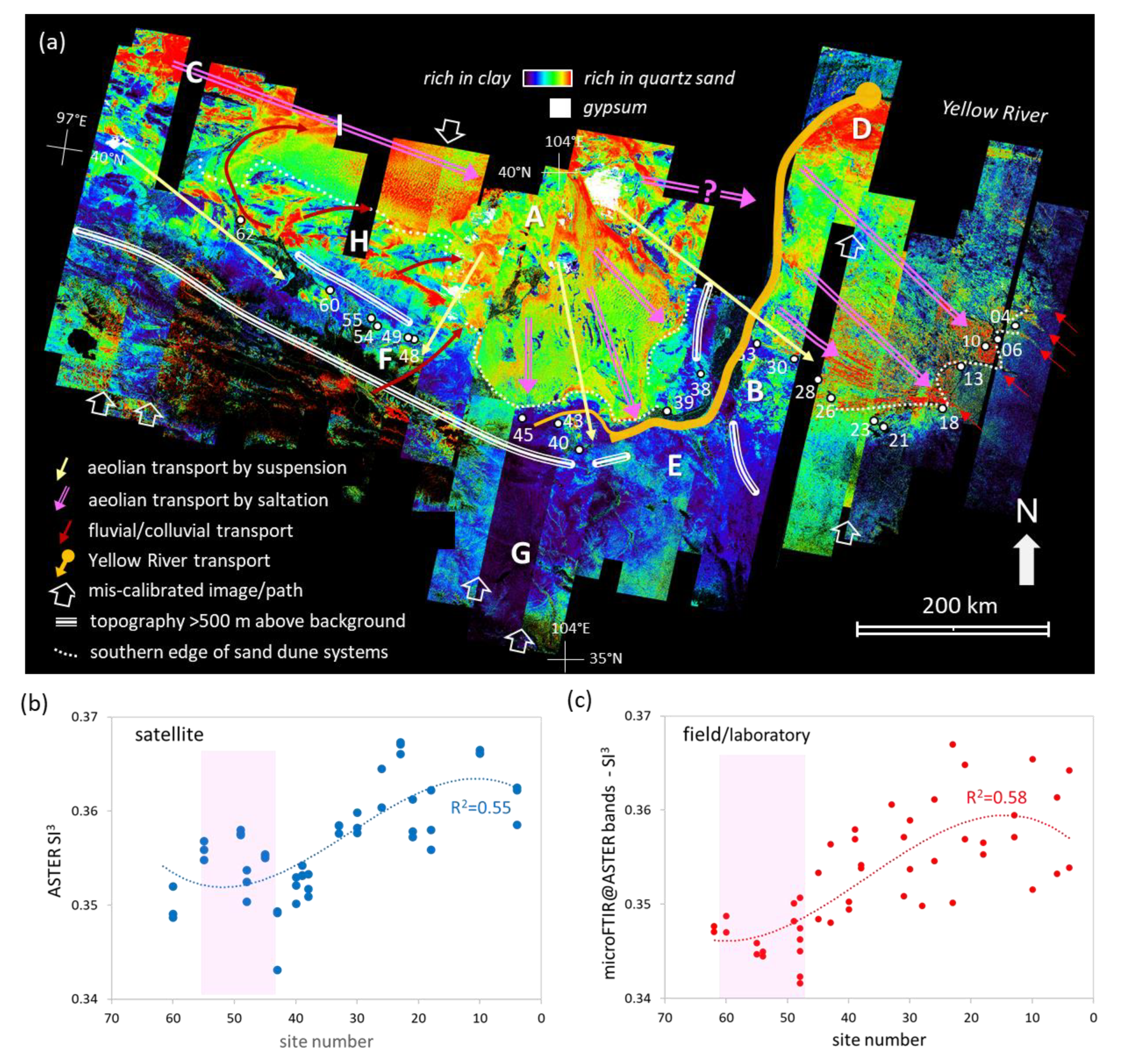
2.13. Interpreting Mineral Transport Pathways

The assumptions used in interpreting the loess system mineral sediment transport pathways include:
  • The loess-related surface materials sensed by the ASTER satellite sensor are either Holocene or possibly late Pleistocene in age.
  • Sediment dispersal (transport) of a given mineral type from its source generates a related decreasing compositional gradient, especially downslope or along flat topography.
  • Reversals in compositional gradients can be caused by sediment “sinks” such as topographic lows or banking-up against topographic highs.
  • The spatial pattern and distance travelled by a particular sediment type is dependent on its particle size and the nature (energy) of the transport process, namely:
    colluvial transport is short (<50 km) and located adjacent to topographic highs;
    fluvial transport is spatially restricted, e.g., within floodplains and (dry) river beds (wadis);
    aeolian transport by saltation is confined to connected lowlands; and
    depending on wind energy and particle size, aeolian transport by suspension can rise above topography and cross-cut fluvial transport networks.
  • The relative timing of transport events, whether they be related to ephemeral rivers or aeolian sand saltation flow, can be assessed by their cross-cutting (compositional) nature.
  • Sand dune patterns have largely developed since the last ice age, i.e., post late-Pleistocene, and thus are a potential indicator of prevailing wind direction/s.
  • Longitudinal sand dunes, which are large amplitude (1–10 km) and often vegetation-stabilized, are formed by prevailing winds operating parallel to the dunes.
  • Transverse dunes, which are small amplitude (~100 m) and typically free of vegetation, are formed by winds operating orthogonal to the dunes.

3. Results

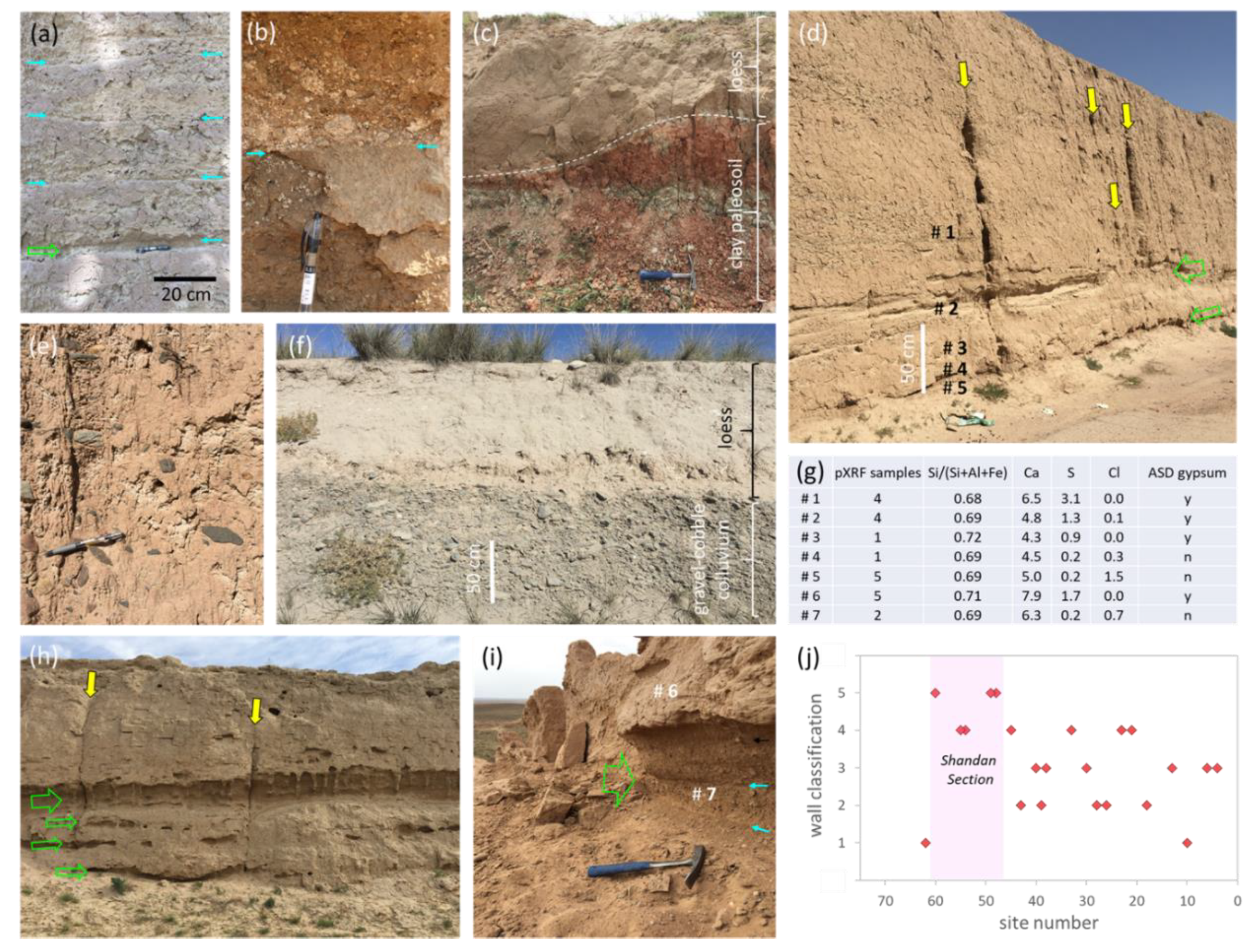
3.1. Earthen Wall Building Materials

All 21 field sites (Figure 1a) showed that the Ming’s “hangtu” method was used to build the earthen border wall, including the characteristic 15–30 cm thick, sub-horizontal layering of loess (Figure 2a). We often found sporadic (<15% by volume) pebbles and cobbles (1–10 cm in diameter; Figure 2b,e) in the wall, especially in areas of thin (<1 m) loess cover. The composition and form of these clasts were similar to local (<100 m) rock fragments exposed on the ground surface or exhumed by nearby building works and road cuttings (Figure 2c,f, respectively). We found loess-type material nearby (<100 m) for all but Sites 38 and 43 (Figure 1a,c), which were built directly on rocky ground in higher relief terrain.

3.2. Earthen Wall Status

Exposed, steep-sided walls often show a variety of erosional characteristics [79]. These include layer-parallel, erosional embayments with widths ranging from 3 to 60 cm (green arrows, Figure 2). The smaller ones (1–3 cm width) are often associated with the 15–30 cm “hangtu” layering (Figure 2a) while the larger ones (5–60 cm) often span a number of these layers (Figure 2h,i) and are usually located <2 m above the wall’s base (Figure 2d,h,i) where not backfilled by aeolian sand (Figure 1d). These embayments can become so recessed that they eventually cause the collapse of the overhanging wall (Figure 2i). Sub-vertical rills (yellow arrows in Figure 2d,h) also contribute to this erosional decay.
The condition of the remnant Ming earthen wall was gauged both visually in the field and digitally using a high-resolution digital elevation model (DEM) generated from drone-acquired, stereo, visible imagery (Figure 1b–e). These different methods yielded similar results though only the visual assessments are presented here. The results (Figure 2j) show a trend of better-preserved wall westward, except for Site 62, which is largely covered by sand dunes. The best-preserved part of the earthen wall is the ~120 km long “Shandan section” (Sites 48–60 and highlighted by a magenta box in Figure 2j).

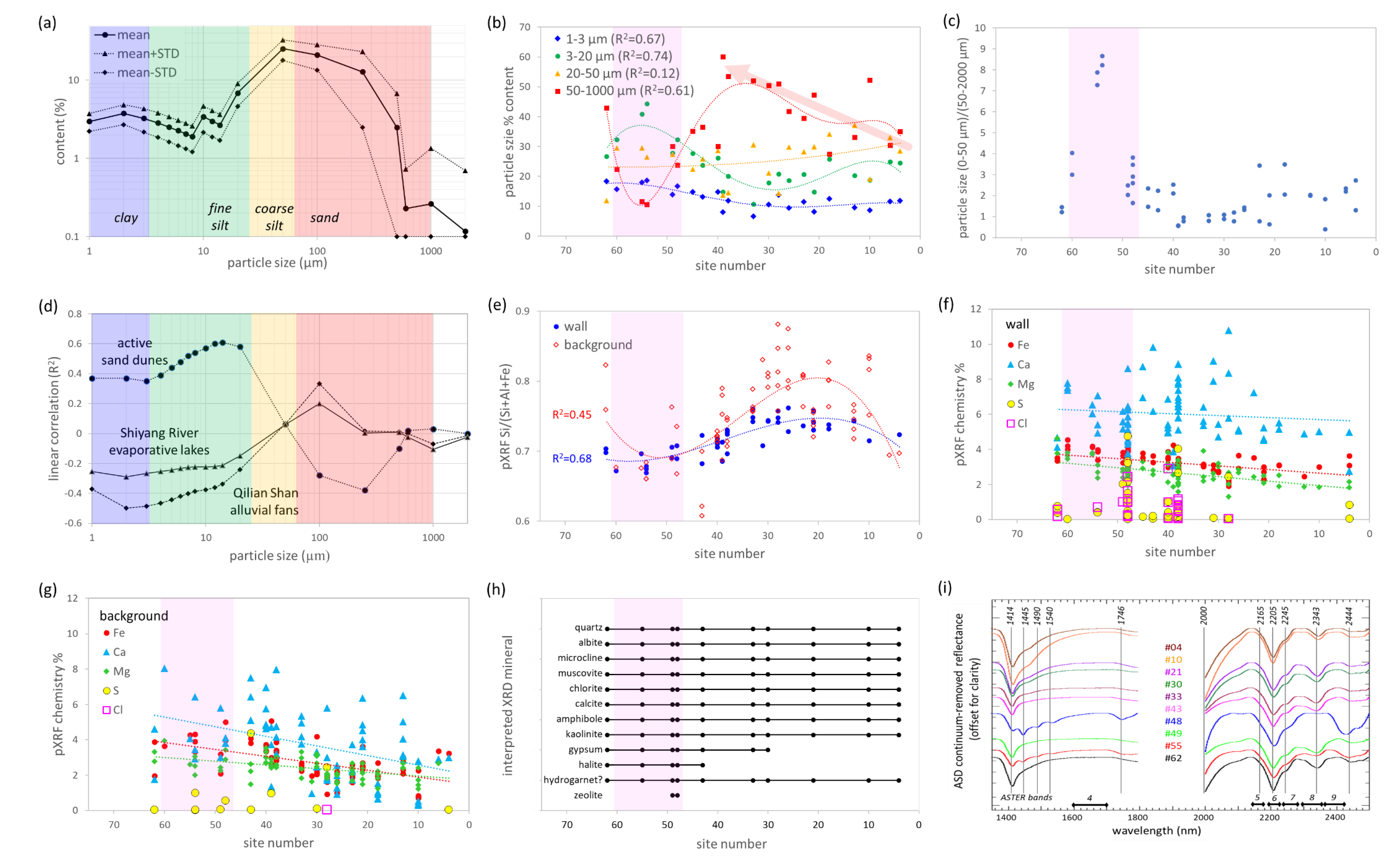
3.3. Loess Particle Size

The particle size of wall material (43 samples from 21 sites) was measured for 19 particle size bins spanning the range from 1 to 1000 µm. The results (Figure 3a) show tight standard deviations (STD ~2%) for all bin sizes ≤100 µm. The volumetrically-dominant bin-size is 20–50 µm (25 ± 7%), i.e., coarse-silt fraction (yellow box, Figure 3a). Combining all of the silt-size bins (2–63 µm) accounts for ~54% of the loess material, whereas sand (>50 µm) represents ~38% and clay (<2 µm) ~8%. This dominance of silt-size grains and left-skewness in particle size distribution (Figure 3a) are characteristic indicators for loess [80]. There is also inverse correlation (R2 = 0.74) between the combined clay and fine-silt fractions (<20 µm) versus the combined sand fractions (>50 µm), given the coefficient of determination (R2) for 21 samples is significant at the 90% confidence level where R2 > 0.57. However, this excludes the 20–50 µm coarse-silt fraction, which yields no improvement when combined with either the finer or coarser fractions. In addition to the main peak at 20–50 µm, there are minor peaks spanning the 0–8 µm (centered at 1–2 µm) and 8–14 µm (centered at 8–10 µm) ranges.
To better understand the spatial pattern of these particle size data, we grouped the particle size bins into four types: (i) 0–3 µm (~clay); (ii) 3–20 µm (~fine-silt); (iii) 20–50 µm (~coarse-silt); and (iv) 50–1000 µm (~sand). Figure 3b shows the coarse-silt group has a relatively flat trend (~25%) along the 1200 km length of the wall. In contrast, the clay and fine-silt groups show smooth-changing curves that vary by a factor of ~2 and are well-modeled using fourth-order polynomials, with minima located near Site 28 and maxima located near Sites 55 (major) and 10 (minor). The 50–1000 µm group is also well-modeled using a fourth-order polynomial and is broadly opposite in pattern to the 1–3 µm and 3–20 µm data, although it also reveals a linear upward trend from Sites 4 (~35%) to 39 (~55%) before rapidly dropping to a minimum at Site 55 (~10%). The well-preserved “Shandan” section of earthen wall (Figure 2j) is associated with this minimum in sand content, where it becomes less than the combined finer fractions. Normalizing all the <50 µm fractions by the combined 50–2000 µm fraction highlights this sand-poor nature of the well-preserved Shandan section of the Ming earthen wall (magenta box in Figure 3c).
To assess possible local (<300 km) sources of the different loess dust components, we measured for each of the 19 particle size bins the distance between a given sample site and three potential source regions: (i) sand dune fields of the Badain Jaran, Tengger, and Mu Us Deserts; (ii) evaporative lakes at the outflow zone of the Shiyang River in the Tengger desert; and (iii) alluvial fans along the northern edge of the Qilian Shan (Figure 1a). Using fitted linear-functions, the results (Figure 3d) show: (i) clay is inversely correlated with the distance from the alluvial fans and to a lesser degree the evaporative lakes and positively correlated with the dune fields; (ii) fine-silt is positively correlated with the sand dunes and to a lesser degree inversely correlated with the alluvial fans and evaporative lakes; (iii) sand is inversely related with the dune fields, albeit weakly; and (iv) coarse-silt shows no relationship. These correlations are improved when fitted with higher order functions. For example, when using a second-order polynomial: (i) clay versus alluvial fans increases up to R2 = 0.74, with the related minima coinciding with the location of the Yellow River; (ii) fine-silt versus sand dunes increase up to R2 = 0.73, with the related minima located ~30 km to the south of the dune-fields; and (iii) sand versus deserts increases up to R2 = 0.43 with the related maximum located ~30 km to the south of the dune-fields. Coarse-silt shows no apparent improvement.

3.4. Field XRF Chemistry—Wall and Background

The pXRF measurements of both wall and background samples show the following spatial patterns: (i) the Si/(Si + Al + Fe) ratio (Figure 3e) approximates a sinusoidal shape for both datasets with their peaks positioned near Site 20 and their inflexion points positioned between Sites 33 and 38 (i.e., where the Yellow River crosses); (ii) the Si/(Si + Al + Fe) ratios for background samples (red diamonds) are ~15% higher than their associated wall samples (blue dots) for localities nearby (<30 km) sandy deserts, i.e., Sites 10–33, 39, and 62; (iii) wall and background samples show a similar trend for Fe and Mg contents which linearly increase westward from 2% to 4% (red dots and green diamonds, respectively, in Figure 3f,g), although wall samples have less variability, (iv) Ca contents are more variable though both wall and background samples show a weak, linear, increasing trend westward (blue triangles in Figure 3f,g); (v) Ca contents of wall samples are on average 2–3% higher than their corresponding background samples (6.0% ± 1.6% versus 3.8 ± 2.2%, respectively); (v) there is a zone between Sites 28 and 48 in wall samples where Ca contents are up ~4% above the general trend of ~6%, which also corresponds to the zone of elevated S; (vi) S contents are typically <0.01% (i.e., below detection limits) for both wall and background samples accept west of Site 28 and especially for a zone between Sites 28 and 48 where S levels can reach up to 5% (yellow circles in Figure 3f,g); and (vii) Cl levels are typically below detection limits (~0.03%) except for wall samples (and one background sample at Site 28) between Sites 28 and 62 where contents are up to 3% (magenta squares in Figure 3f,g).
At a site-scale, the field pXRF measurements show considerable heterogeneity and differences between chemical elements down a given vertical section of the wall. For example, at Site 48 (Figure 2d), S decreases from 3.1% at ~2 m above ground (#1 in Figure 2d,g) to 0.2% at ~30 cm above ground (#5 in Figure 2d,g). Similarly, Cl also shows considerable variability. For example, at Sites 48 (Figure 2d) and 38 (Figure 2i), Cl measurements from within (e.g., #2, #5, and #7) and immediately adjacent (<15 cm, e.g., #4) to wide (15–50 cm), sub-horizontal embayments (green arrows in Figure 2d,h,i) yield high (0.1–3.1%) values (Figure 2g). Away from these eroded layers (e.g., #1, #3, and #6), Cl values are below pXRF detection limits. In contrast, the Si/(Si + Al + Fe) ratio remains constant throughout.
We interpret these pXRF as follows: (i) the similarity between the Si/(Si + Al + Fe) chemistry (Figure 3e) and particle size distribution (Figure 3b,c) is driven by a change in composition across the spectrum of particle sizes, namely Si-rich (i.e., quartz) coarser fractions to Al-rich (i.e., white mica, kaolinite) and/or Fe-rich (e.g., chlorite) finer fractions; (ii) Fe and Mg are related to the mineral chlorite [(Fe2+,Mg,).5Al2Si3O10(OH)8], which was sourced from the west (up gradient); (iii) the similar patterns for wall versus background samples for Si/(Si + Al + Fe) (Figure 3e) as well as Fe, Mg, and S (Figure 3f,g) are evidence that the Ming locally (~100 m) sourced the loess to build their earthen wall; (iv) the lower Si/(Si + Al + Fe) values of wall samples versus their associated background surface samples nearby sand deserts is evidence that the Ming had developed methods to assess and selectively mine loess poor in quartz-sand content; (v) the low variability of Fe for wall (1 STD = 0.6%) versus background samples (1 STD = 1.0%) is evidence that the Ming used visual color for grading the quality of the loess, given that Fe is contained in either chlorite (green/brown) or related weathering products, namely hematite (red) or goethite (yellow); (vi) the elevated S contents west of Site 28 in both wall and background samples (yellow circles in Figure 3f,g) is related to gypsum (CaSO4.2OH), which is aeolian in origin and derived from evaporative lakes in the Tengger Desert; (vii) the relative lack of Cl in background surface samples but common occurrence in wall materials west of Site 28 can be explained by aeolian halite (Na.Cl) derived from a nearby source (e.g., evaporative lakes in the Tengger Desert) that is readily leached from the surface into the groundwater where it then can be mobilized, presumably by capillary action, up into specific “hangtu” layers of the wall; and (viii) the consistently higher Ca content of wall samples versus background samples is evidence that the Ming routinely applied a Ca-rich additive, most likely lime.

3.5. XRD Mineralogy—Selected Wall Samples

Ten wall samples were measured using laboratory X-ray diffraction (XRD), namely Sites 4, 10, 21, 30, 33, 43, 48, 49, 55, and 62. The mineralogy interpreted from these whole-sample analyses include: quartz, albite, microcline, muscovite, chlorite (chlinochlore and chamosite), kaolinite, calcite (no dolomite), amphibole (actinolite), gypsum, halite, poorly crystalline, hydrated clay (~montmorillonite and/or interstratified clay), a zeolite, and possibly a hydrogarnet. We determined muscovite rather than illite in these bulk sample XRD analyses given the 10 Å peak-width at half-height-maximum (FWHM) is <0.2 Å. The zeolite mineral, laumontite [Ca(AlSi₂O₆)₂·4H₂O]), was identified by peaks at 9.46 Å and 6.83 Å (Sites 48 and 49). Similar to the pXRF Ca, Cl, and S results (Figure 3e), gypsum, halite, and laumontite were only detected by XRD west of Site 28 (Figure 3h). All samples show a number of other minor but difficult to interpret XRD peaks, including one at 2.64 Å, which is possibly related to a Ca-bearing hydrogarnet.

3.6. Field and Satellite VNIR-SWIR Results

Selected field ASD spectra of wall loess samples taken from the same sites chosen for the XRD analyses (Figure 3h) are presented in Figure 3i. Absorption by water vapor (and surface water) is masked out between 1800 and 2000 nm. These wall loess samples are all intimate mixtures of minerals, including: muscovite (2200, 2350, and 2450 nm); illite (2200, 2350, 2450 nm, and well-developed water related shoulder near 2000 nm); chlorite (2000, 2245, and 2330 nm); and gypsum (1445, 1490, 1540, 1746, 2215, and 2410 nm). Kaolinite (2165 and 2205 nm) and calcite (2335 nm) are more difficult to recognize, although kaolinite is identified because of a characteristic sharp absorption locked in at 2205 nm (~18 nm FWHH, whereas the muscovite and illite absorption is >30 nm width and can vary in wavelength [52]) and a depressed shoulder near 2165 nm, as shown by ASD spectra from Sites 43–55 (excluding Site 48). This subtlety reflects the fact that kaolinite represents only a minor component of the loess compared with minerals such as muscovite.
The mineral information targeted using ASTER’s moderate spectral-resolution capabilities (Figure 3h) included: (i) the presence of gypsum; (ii) the proportion of quartz sand versus clay (called sand-clay index or SI3); (iii) the content of silicate minerals such as kaolinite and white mica (called 2200D); (iv) the proportion of kaolinite versus white mica and/or montmorillonite (called 2165D); and (iv) the combined content of chlorite, carbonate and/or amphibole (called 2330D). We validated these ASTER mineral maps using coincident ROIs of the field ASD data convolved to ASTER responses. Full-spectral resolution field ASD were also used where required to more accurately interpret the composition of the mineral components.

3.6.1. Gypsum

The full spectral resolution field ASD data show diagnostic gypsum absorptions at 1446, 1490 and 1540 nm for wall samples collected from Sites 40, 48 (Figure 3i), 55 (Figure 3i), 60, and 62 and background surface samples collected at Site 43 only. Thus, the ASD, XRD, and pXRF data all indicate a similar pattern where gypsum is present in a zone spanning Sites 28–62.
The ASTER gypsum index [61] was clipped to identify pixels most likely to contain gypsum. The resultant map (white filled polygons in Figure 4a) reveals numerous, large (up to 50 km wide) occurrences of gypsum associated with evaporative lakes. Most of these ephemeral lakes are found in the Tengger Desert (“A”), with less in the Badain Jaran Desert and no apparent gypsum occurrences are evident in the Mu Us and Hobq Deserts, at least at this map-scale (Figure 4a).
We propose that northerly to westerly winds (light yellow arrows in Figure 4a) transported gypsum-laden dust as long-term suspension from evaporative lakes in the Tengger and Badain Jaran Deserts to areas <300 km away. We also suggest that this gypsum-laden dust was able to cross topographic highs of the Helan Shan and the Alashan Block (Figure 1a and Figure 4a).

3.6.2. Sand-clay Index

The SI3 index is sensitive to the abundance of sand rich in quartz (and other silicates such as feldspars) relative to clay materials (size and composition) and is driven by the wavelength and intensity of the silicate reststrahlen feature near 8.6 µm [70,81]. The satellite and field SI3 data show similar sigmoidal patterns (Figure 5a,b, respectively) that are well-modeled using third-order polynomials and are consistent with the pXRF Si/(Si + Al + Fe) results (Figure 3e). All show inflexion points positioned between Sites 33 and 39 (i.e., approximate position of the Yellow River), with quartz-sand-rich materials to the east and clay-rich materials to the west. Similar to the particle size results, which show that the loess along the Shandan section is poor in sand (Figure 3c), the associated field SI3 values are also at their lowest, i.e., least amount of quartz sand (Figure 4c).
The ASTER SI3 map (Figure 4a) depicts areas rich in quartz-sand as warmer tones while areas rich in clays are cool tones. The two areas most abundant in quartz-sand are parts of the Gobi Desert (near “C”) and the Hobq Desert (“D”). From the limited spatial coverage selected for our study area, we recognize SI3 gradients extending away from these enriched zones as follows. The area of highest SI3 values in the Gobi Desert (near “C”) is located over terrain comprising exposed Mesozoic and Cainozoic sedimentary rocks, including Cretaceous sandstones. From here, the SI3 progressively decreases east-southeastward (i.e., the direction of quartz-sand transport) along a linear ~500 km long trajectory (“C” to “A”), paralleling (restricted by) the highlands of the Alashan Block to the south (“H”). In the process, this SI3 signature seamlessly crosses the >40 km wide wadi of the Heihe River (Figure 1a). That is, this aeolian activity is sufficiently frequent to obscure the potentially cross-cutting effects of fluvial sediment transport.
Continuing eastward from the Heihe River wadi, the SI3 signature extends down-gradient for ~100 km across dune-fields of the Badain Jaran Desert, which comprise linear to complex dune patterns consistent with an easterly flow of quartz-sand mobilized by saltation. The SI3 gradient then begins to increase for ~100 km across similar dune-fields concomitant with a rise in topography (100 m), reaching a maximum height along the Yabra Shan (Figure 1a). Beyond here, the pathway of quartz sand transport becomes more diffuse as it enters the lowland expanse of the Tengger and Ulan Buh Deserts (Figure 1a). The SI3 map also provides evidence for the input of quartz sand into this desert pathway from the Qilian Shan (“F”) and Alashan Block (“H”), although we suggest this sediment was mobilized downslope chiefly by fluvial and/or colluvial processes (dark red arrows in Figure 4a).
The SI3 gradients across the Tengger Desert are more variable, which is consistent with the complex pattern of linear dune systems, both longitudinal and transverse. The net result is a saltation movement of aeolian quartz sand (magenta arrows) that terminates against the Yellow River or its ephemeral tributaries (e.g., between Sites 39 and 45, Figure 4a). Importantly, the ASTER SI3 values markedly step-down along this boundary, which is clear evidence for aeolian saltation flow. That is, quartz sand has not been transported by wind-suspension across the river to be deposited some distance across on the opposite bank near, e.g., near “E”.
Thus, the entire volume of quartz sand flowing by aeolian saltation through the Tengger Desert, and presumably Ulan Buh Desert, is consumed by the Yellow River before being transported downstream (thick orange arrow). This is consistent with field studies which have found a pronounced increase in the sand sediment load along this section of the Yellow River [81,82,83,84] and corresponds to a change in flow regime from a deep, meandering channel upstream to a shallow, braided system downstream that extends along the margin of the Hobq Desert. It then returns to a single, deep channel, presumably because the river’s load of sand has been deposited.
The SI3 pattern across the Ordos Plateau is less complex, driven largely by southeastward saltation of quartz sand (magenta arrows) paralleling longitudinal dunes in the southern half of the Mu Us Desert. The highest SI3 values are located in a ~50 km wide, lens-shaped zone spanning vegetation-free, transverse dunes (<100 m amplitude) of the Hobq Desert (“D” in Figure 4a). Southeastward from here the SI3 gradient decreases for ~100 km values before gradually increasing over the Mu Us Desert concomitant with the development of longitudinal dunes. A series of quartz sand rich incursions or cusps (red arrows) extend for >30 km southeastward into the zone of loess. These cusps appear not to be constrained by topography as they are located over both shallow valleys and low hills. In contrast with the sharp southern boundary of the Tengger Desert, the southern margin of the Mu Us Desert (white dotted line in Figure 4a) shows a diffuse SI3 transition with the adjacent loess deposits across a ~50 km zone.
There is no indication from the SI3 map (Figure 4a) that the upper catchment of the Yellow River (west of “G”) in northeast part of the Tibetan Plateau was a significant source of quartz sand. This contrasts with the Qilian Shan near “F”, which has both exposed rocks and associated downslope fans and alluvial plains of the Shiyang River with characteristically high SI3 values.

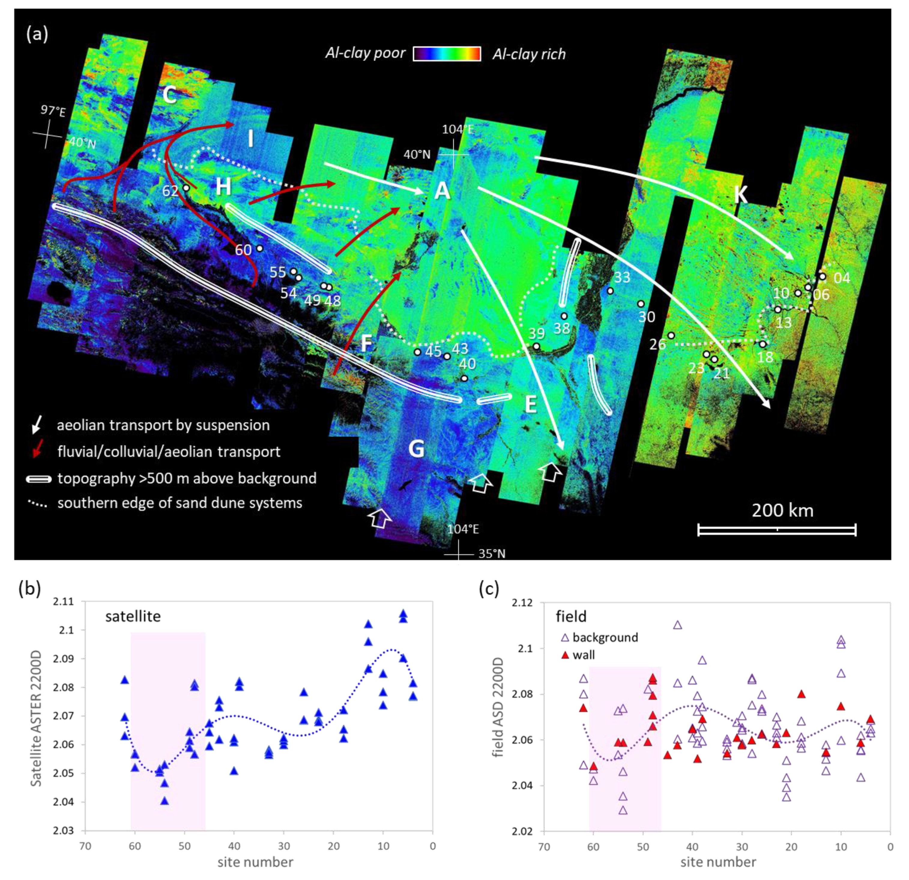
3.6.3. Al-Clay Content Index

Both the field and satellite 2200D data show similar weak patterns which are modeled here using fifth-order polynomials. These show a narrow low centered near Sites 55 and 56 (Figure 5b,c), which is coincident with the zone poor in (quartz) sand size material (Figure 3c). This association helps to explain this apparent 2200D low as the lesser amount of optically-transparent quartz grains reduces the overall optical thickness, resulting in less opportunity for electromagnetic radiation to interact with clay mineral particles [75,76]. This optical transparency effect also helps explain why the quartz-rich dune-fields (Figure 5a) have moderate to high 2200D values (warmer tones) even though they generally contain less clay mineral content compared with loess (Figure 3b,e and Figure 5b,c). One exception, however, is the western part of the Badain Jaran Desert (“I”), which has a low 2200D response that seamlessly merges with the wadi of the Heihe River and not the nearby Gobi Desert (“C”) or the Alashan Block (“H”). Instead, we trace the source rocks up the Heihe River to areas of low 2200D signature along the western part of the Qilian Shan, i.e., south of Sites 54–62. Similarly, the higher 2200D response of the eastern half of the Badain Jaran Desert can be traced to sediment eroded from the Alashan Block (dark red arrows in Figure 5a).
Further east along the Qilian Shan, there are rock exposures near “F” (Figure 5a) that generate the highest 2200D responses across the study region. This high response then persists downslope across associated alluvial fans and then along the Shiyang River wadi before merging seamlessly into the Tengger Desert (dark red arrow). In contrast, the upper reaches of the Yellow River catchment (near “G”) comprise a relatively low 2200D signature, although it does increase downstream near “E”, where it seamlessly merges with the 2200D signature of the Tengger Desert. This signature can be traced southward across the Yellow River and over loess deposits for >100 km (“E”), although appears to be constrained (given image miscalibration error) by the eastward extension of the Qilian Shan, where topography is >500 m above background (triple white lines). This apparent lack of 2200D contrast between dune-fields and loess is also evident across the Ordos Plateau between the Mu Us Desert and loess to its south (between Sites 4 and 26 in Figure 5a).

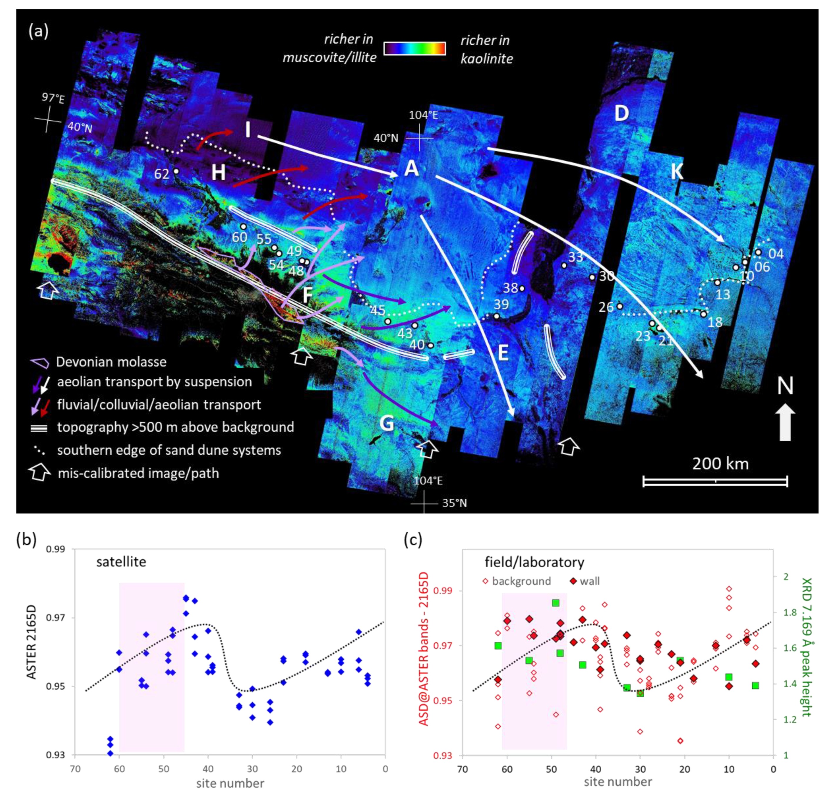
3.6.4. Kaolin—White Mica Index

The ASTER 2165D is sensitive to the composition of dioctahedral clay minerals with kaolinite generating a higher response and white mica a lower response, although this interpretation is most appropriate for those areas sharing a similar 2200D response. Both the field and satellite ASTER 2165D data show a similar sigmoidal (dextral offset) pattern (Figure 6b,c, respectively), with the Yellow River valley (Sites 33–39) marking the inflexion point. That is, there are higher levels of kaolinite relative to white mica (high 2165D response) in the zone between Sites 40 and 48 in background samples, whereas there are higher levels of white mica to kaolinite in the zone between Sites 26 and 33. This pattern is broadly consistent with the height of the kaolinite related XRD peak at 7.169 Å (green squares in Figure 6c). Wall samples along the well-preserved Shandan wall section tend to be rich in kaolinite, although the associated background samples are more variable (Figure 6c). This is related to the fact that background surface samples were not always available from exposed loess but instead either alluvium (e.g., Sites 49, 54, and 55) or sand dunes (e.g., Site 62).
The satellite 2165D map (Figure 6a) shows areas richer in kaolinite as warmer tones. Regionally, kaolinite is more abundant over the Tibetan Plateau with some of the highest 2165D responses associated with Devonian molasse in the Qilian Shan (purple polygon). These exposures have associated downslope colluvial/alluvial aprons (light purple arrows in Figure 6a). However, aeolian transport by long-term westerly wind suspension (dark purple arrows in Figure 6a) is also required to account for the 2165D gradient that extends for up to 300 km eastward across to the southern parts of the Tengger Desert and the upper Yellow River catchment (“G”).
The lowest 2165D responses (cooler tones, i.e., rich in white mica) are found over the Badain Jaran Desert (I) and the Alashan Block (“H”). We propose that the eroding geology of the Alashan Block is a (the) primary source of white mica with derived sediments initially transported downslope by colluvial/alluvial processes before entering the aeolian sediment transport pathway along the Badain Jaran and then ultimately the Tengger and Ulan Buh Deserts. The associated low 2165D response then crosses southward across the Yellow River into loess deposits near E as well as eastward to the Ordos Plateau. However, the 2165D gradient then increases eastward, which could be a function of increased weathering related to higher rainfall in this region resulting in the formation of kaolinite after minerals such as chlorite and feldspar [85]. Given this apparent, mildly elevated level of kaolinite across the Ordos Plateau is caused by weathering, the dominant white mica component is likely transported by long-term wind suspension uplifted from the Badain Jaran and Tengger Deserts (white arrows) with related particles originating from source rocks exposed across the Alashan Block (“H”).

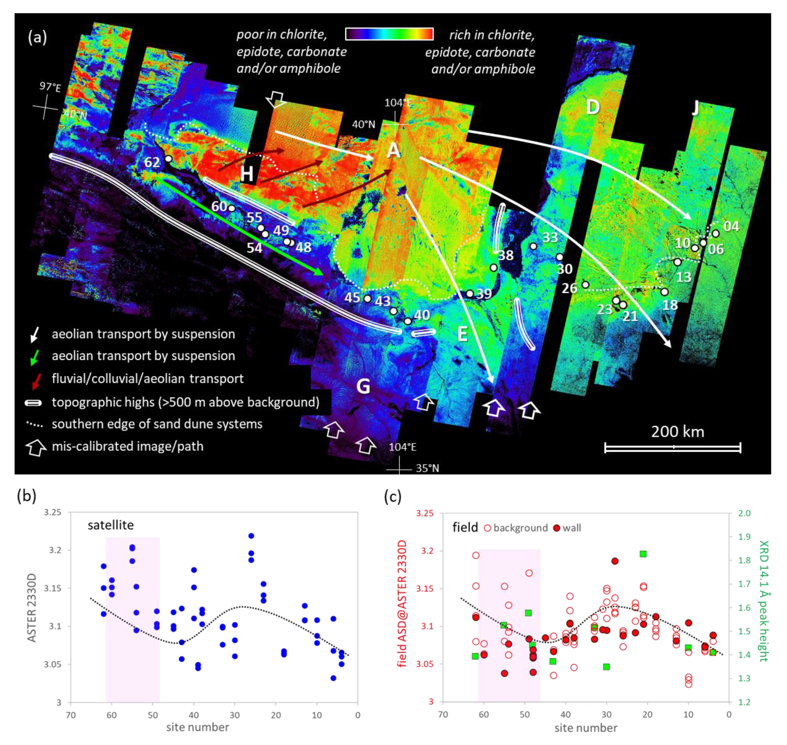
3.6.5. Chlorite/Carbonate/Amphibole Content

We identified chlorite as the dominant 2330D absorbing mineral from the field ASD spectra based on absorptions at around 2000, 2250, and 2230 nm. Both the satellite and field 2330D data show a similar sigmoidal (sinistral offset) pattern (Figure 7b,c, respectively), that is opposite to that observed with the 2165D data (Figure 6b,c). However, all share a similar position for their inflexion point, which is located over Yellow River valley (Sites 33–40). Wall samples along the well-preserved Shandan section are relatively poor in chlorite and less variable compared with their associated background samples (Figure 7c), which often comprise colluvial/alluvial material (e.g., Sites 49, 54, and 55).
The satellite 2330D map (Figure 7a) shows areas richer in chlorite as warmer tones. The highest 2330D responses are found on the Alashan Block (“H”) from which stems a seamless, decreasing gradient spanning the eastern part of the Badain Jaran Desert and then across the Tengger Desert (“A”) before dispersing across the Yellow River southeastward towards “E” and eastward over the Ordos Plateau. The lack of a 2330D north–south gradient across the Ordos Plateau is evidence that the source of these aeolian-borne trioctahedral minerals were not local but from a distant region. The low 2330D signatures that characterize the Tibetan Plateau, loess deposits in the upper reaches of the Yellow River (“G”), the Qilian Shan, Hexi Corridor, and Heihe and Shiyang Rivers (Figure 1a and Figure 7a) indicate these areas are not intrinsic to the chlorite (and carbonate and other trioctahedral minerals) mineral transport pathway. We thus interpret the 2330D transport pathway from source to loess deposition as initially being downslope, colluvial-fluvial movement from source rocks exposed across the Alashan Block (dark red arrows) before being entrained by westerly to northwesterly wind long-term suspension (white arrows) that deliver chlorite to distant (>500 km) areas including loess deposits of the Ordos Plateau (Figure 1a).

4. Discussion

We have presented here a range of evidence that shows the Ming earthen wall changes in composition along its 1200 km length between Shenmu and Jiayuguan (Figure 1a). These compositional changes are apparent in field sample measurements of wall samples and nearby surface background materials (Figure 3b,c,e–h, Figure 4c, Figure 5c, Figure 6c, and Figure 7c) and are consistent with the ASTER surface mineral maps and related ROI data (Figure 4a,b, Figure 5a,b, Figure 6a,b, and Figure 7a,b). All show that the loess used by the Ming to build their earthen wall is compositionally heterogeneous. This has implications for improved understanding of: (i) where the Ming mined loess to build their earthen wall; (ii) the origin of the loess materials; and (iii) the importance of mineral composition in determining the wall’s long-term erosional durability.
In addition to the similarity in composition (mineralogy and chemistry) between wall and background (<50 m away from the wall) materials (Figure 3e–g, Figure 4b,c, Figure 5b,c, Figure 6b,c, and Figure 7b,d), there is also the similarity in the nature of rock fragments (where available) at a given site. We cite these as key evidences for the Ming sourcing their earthen wall building material from nearby (<500 m), surficial (<30 m depth) loess deposits of presumably Holocene or possibly late Pleistocene (i.e., Malan loess units) age. We conjecture that, where available, the Ming’s inclusion of up to 20% local rock fragments into the wall building material (Figure 2b,e) simply served as an expedient additive rather than being designed for improving the wall’s structural performance, unlike previous Dynasties such as the Han who incorporated layers of rock into their wall design, i.e., were a mixture of both grain (=rock) supported as well as matrix (=loess) supported.
We further propose that the Ming established at least three methods to improve the quality of the loess for their earthen wall construction. The first is that they routinely gauged the sand content of the loess and, if required, selectively mined deeper loess layers richer in silt and/or clay content if required (Figure 3e). This would have been particularly important across the Ordos Plateau where incursions of saltating sand grains regularly occurred because of a lack of physical barriers such as vegetation, mountains, and permanent rivers. At the same time, it was fortuitous for the Ming that the limited depth of loess across the Hexi Corridor (~1 m layer, Figure 2f) was of high-quality building material rich in finer fractions (Figure 3c,e and Figure 4c), else they would have had to either transport loess from mines located a great distance away or found an alternative locally-available building material, much of which has a high content of rock. Similarly, we propose that the Ming used color, which is related to the content of iron oxide and/or chlorite, to assess the quality or at least maintain consistency of the mined loess (Figure 3f).
The third method we propose is that the Ming applied a Ca-rich material, possibly calcite but more likely lime. This is based on the consistent ~2% higher levels in Ca content of wall versus background materials across the study area (Figure 3f,g, respectively). The lack of a similar pattern for both Mg and S indicates that neither dolomite [(Ca,Mg)CO3] nor gypsum was involved. Lime was well known to the Ming having been used in construction back to the Shang Dynasty (1700–1027 BC) [2]. In theory, a 2% lime application rate is sufficient to reach the “lime fixation point” where ions are absorbed by clay minerals, which increases the unconfined compressive strength of the earthen material [86]. After this point, alkali activation can cause the (re)precipitation of calcite as part of a pozzolanic type reaction [54]. However, nano-fibers of secondary calcite are also found in natural loess material [48] such that (re)crystalized calcite in the earthen wall material is not itself conclusive evidence for lime addition by the Ming.
The advanced stages of pozzolanic reaction generate a variety of Ca-bearing silicate and/or alumino-silicate minerals, such as ettringite, tobermorite, zeolites, and hydrogarnets [17,86]. From our limited XRD data, we detected the zeolite mineral, laumontite, at Sites 48 and 49 (Figure 3h). Given that zeolites can also form by subaerial dissolution of silicate minerals in a range of geologic environments at near-surface conditions [87], its limited distribution is unlikely to be the result of systematic application of lime by the Ming. Instead, we suggest its overlapping pattern with gypsum and halite (Figure 3h) is the result of aeolian transport from nearby evaporative lakes (Figure 4a). From the available data, we are not confident that hydrogarnet or any other Ca-bearing alumino-silicate cementing minerals are present in the wall material. Thus, even though we conclude that the Ming added ~2% Ca, most probably lime, to their loess building material, this may only have had the intended effect of improving its compressive strength rather than generating a binding cement.
Previous studies have been unable to agree on the sediment transport pathways that generated the vast loess deposits across north-central China [21,22,23,24,25,26,27,28,29,30,31,32,33,34,35,36,37,38,39,40,41,42,43,44,45,46,47,48,49,50]. We suggest that this lack of consensus is a function both of the complexity of the loess system and the limitations of the analytic tools and sampling strategies used to date. Similar to the parable of the elephant and the six blind men, only when one can see the bigger picture is it possible to begin to resolve the relationship of the parts. We argue that our use of satellite ASTER mineral maps has assisted in untangling this complexity by enabling a view of the “whole”, at least for a few mineral components of the loess. To that end, Table 1 lists the essential ingredients and mappable criteria [53] we conclude are valuable for mapping the “loess system” using ASTER’s limited but valuable spectral/spatial/radiometric resolution.
Using the ASTER mineral maps (Figure 4a, Figure 5a, Figure 6a, and Figure 7a), we identify at least two sediment transport pathways, both of which source mineral grains from a variety of exposed rocks. These two pathways or “loess subsystems” are driven by their grainsize energy potential: (i) sand; and (ii) clay to fine-silt (Table 1).
The transport pathway for the quartz sand fraction (>50 µm), which accounts for ~40% of the loess material (Figure 3a,b), is initially driven by colluvial/alluvial downslope movement from source rocks in the Gobi Desert, Alashan Block, and Qilian Shan (dark red arrows in Figure 4a). There could also be a significant amount of quartz sand originating from rocks to the north and/or west of the limits of the current study area. The quartz sand then travels by aeolian saltation flow along lowlands of the Badain Jaran, Tengger, and Ulan Buh Deserts (magenta arrows in Figure 4a) forming arrays of multi-scale linear dunes systems. Most of this quartz sand is then consumed by the Yellow River and delivered downstream to where it is then deposited along the banks of the western Mu Us and Hobq Deserts (thick orange arrow). It then becomes available for transport by northwesterly wind saltation flow before finally depositing along the northern margin (<100 km wide) of the loess plateau. Related ASTER SI3 gradients change over distances of <300 km determined by distance from “source” and topography. A gentle rise of even 1:1000 appears to retard saltation flow causing a bank-up (deposition) of quartz sand, resulting in a reversal of the SI3 gradient. An example is the eastern part of the Badain Jaran Desert (between “I” and “A”), which has the highest star dunes (~500 m high) in the world. A greater rise in topography to 1:100 appears to inhibit the saltation flow of quartz sand, as demonstrated by the western flank of the Helan Shan Figure 1a and Figure 4a). These observations help explain why the loess developed along the Hexi Corridor is relatively poor in quartz sand because of shielding by mountains of the Alashan Block from quartz sand moving by north-northwesterly wind saltation along the Badain Jaran Desert (Figure 5a).
The transport pathway for the combined clay and fine-silt fraction (<20 µm), which accounts for ~30% of the loess material (Figure 3a,b), is characterized by aeolian long-term suspension with related sediment travelling for many hundreds of kilometers, often at high elevation (>2000 m). We identified several rock sources of these finer particles in our study area using the ASTER indices (Table 1): (i) gypsum (SI3 index) from evaporative lakes in the Tengger Desert (Figure 4a); (iii) kaolinite (2200D and 2165D indices) from Devonian Molasse in the Qilian Shan (Figure 5a and Figure 6a); and (iv) chlorite (2330D index) and muscovite (2200D and 2165D indices) from the Alashan Block (Figure 5a, Figure 6a, and Figure 7a). Previous mineralogical work across the Chinese Loess Plateau on the Malan Loess Unit [88,89] found that the dominant minerals of the fine-silt fraction comprise quartz (~30%), muscovite (~27%) and chlorite (~22%) while the clay fraction comprises illite (~46%), kaolinite (~16%), and chlorite (~15%). This mineralogical distinction according to particle size is consistent with our spectral results. That is, both muscovite and chlorite share the same sediment transport pathway, originating primarily from source rocks in the Alashan Block by colluvial/fluvial processes (dark red arrows in Figure 5a, Figure 6a, and Figure 7a) before being uplifted by westerly to northwesterly wind long-term suspension (white arrows in Figure 5a, Figure 6a, and Figure 7a) to eventually be deposited in areas >500 km away, including the Chinese Loess Plateau. This shared transport pathway is expressed as a continuous down-gradient in the ASTER 2165D (dark blue to cyan in Figure 6a) and 2330D (red to yellow to green in Figure 7a) maps. It is also expressed as a southeastward decrease in chlorite and muscovite content of the loess developed across the Ordos region [34,46,48]. These observations are consistent with both muscovite and chlorite being significant components of the fine-silt fraction.
We trace kaolinite using the ASTER 2200D and 2165D maps back to source rocks in the Tibetan Plateau, including Devonian Molasse exposed along the Qilian Shan (Figure 5a and Figure 6a). However, this kaolinite comprises a range of particle sizes given that it shows a 2165D gradient spanning <500 km north/east from “F” and with characteristics of both downslope colluvial/alluvial transport, associated with fans and ephemeral drainage networks (mauve arrows in Figure 6a), and aeolian dispersal across the southern parts of the Tengger Desert and western loess plateau (dark purple arrows in Figure 6a). Note that this “primary” kaolinite is different to the “weathering” kaolinite in the southeastern part of the study area, which has been identified by other workers [13,34,85] and suggested to be related to increasing rainfall.
In addition to the “sand” and “clay to fine-silt” subsystems described in Table 1, we also acknowledge the existence of other sediment transport systems contributing to the development of loess: (i) “clay”; and (ii) “coarse-silt”. The coarse-silt fraction (20–50 µm), which accounts for ~30% of the loess material, shows no coherent spatial pattern along the length of the Ming earthen wall (Figure 3b). It also does not yield any statistical association with other particle size fractions or targeted source areas (Figure 3d). Given that U-Pb studies [24,30,31,37], which measure zircon grains of >30 µm size (i.e., coarse silt size), have consistently concluded that the Yellow River is sourcing a significant amount of material from the Tibetan Plateau (and adjoining Qaidam Basin), we suggest that the Yellow River is transporting the bulk of this coarse-silt sediment through the study region. The mineralogy of this coarse-silt likely includes plagioclase, alkali feldspar, and amphibole [31,88]. Similar to the sand fraction, a significant part of this coarse-silt material is deposited alongside the Hobq Desert before mobilization southward by aeolian saltation where it is finally incorporated into loess. The thickest part of the Malan Loess Unit (Figure 1a) reflects this south(east)ward flow of coarse-silt (and sand) originating from the banks of the Yellow River during the late Pleistocene and most likely through the Holocene [8].
Clay-size grains, which can travel distances of 1000s of kilometers by long-term wind suspension [8,47,89], are also readily transported by fluvial suspension. The Yellow River, which carries the largest volume of sediment of any river on the Earth [90], owes its distinctive beige-yellow color to a mixture of suspended clay minerals and iron oxides. Much of this suspended clay material is deposited into marine environments >1000 km to the east of the study area. Drill cores sampled from the Bohai and Yellow Seas [90] show that the clay-size mineralogy comprises: illite (average: ~60%), smectite (average: ~15%), chlorite (average: ~15%), and kaolinite (average: ~10%). This dominance of illite in the clay fraction is mirrored in the Malan loess unit [8] found across the Ordos region (Figure 1a). Illite formation is unlikely to occur through regional weathering because at surface temperatures the crystallization of illite requires a specific range of Si and K activities usually found in saline environments [91]. That is, illite is more likely to have formed in evaporative basins, such as parts of the Tengger, Badain Jaran, and Taklamakan Deserts [25,92,93]. The Taklamakan Desert has been identified as a key source of clay size material transported by long-term westerly wind suspension to the Ordos region [33,40,41,93].
The Ordos Plateau region thus represents a depositional “cross-road” for at least four sediment transport pathways. This contrasts with the Hexi Corridor which lacks significant contributions of sand associated with the Badain Jaran aeolian saltation pathway as well as coarse-silt associated with the Yellow River pathway. This has resulted in the loess developed along the Hexi Corridor being relatively abundant in clay and fine silt (Figure 3c) and with a composition relatively poor in quartz (Figure 3e and Figure 4c) and richer in kaolinite (Figure 6c) because of its proximity to kaolinitic source rocks in the Qilian Shan (“F” in Figure 5a and Figure 6a). These factors have likely driven the relative erosional robustness of the Ming’s earthen wall along the Shandan section (Figure 2j), because of greater opportunity for hydrogen bonding between water molecules and the surfaces of the finer mineral grains [16].
Groundwater penetration along specific “hangtu” layers continues to generate a cycle of crystallization and dissolution of salts, resulting in erosion and undercutting of the wall (Figure 3i) [94]. We observed in the field that when irrigated farming abutted the wall, then the erosion immediately above was dramatically enhanced compared with the wall <10 m away from the edge of the cropped field (e.g., at Site 49, 38°19.952′N; 101°54.259′E). Thus, the control of groundwater movement is crucial in the continued preservation of the earthen wall.
ASTER has proven valuable for mapping and understanding the complexity of mineral-composition patterns not apparent in point-sample field data alone. In so doing, ASTER has enabled us to build a “loess system” model for at least two sediment transport pathways. However, ASTER’s modest spectral resolution (compared with hyperspectral systems) has impacted what loess mineral information can be targeted. Higher spectral resolution systems with tens to hundreds of spectral bands should in theory provide more detailed compositional information and thus improve the accuracy and detail of this loess system analysis. For example, the Tschermak chemical composition of both muscovite and chlorite can be measured and traced back to more specific rock sources [52].
NASA’s hyperspectral VNIR-SWIR EMIT imaging system, which is scheduled for operation starting 2020 on board the International Space Station (ISS) [95], is one candidate, especially given that it has the task of mapping the surface mineralogy of dust generating regions of the Earth to assist in global climate models. It is a shame that ASTER was not also tasked to help deliver this important information, especially given its 20-year archive of multi-temporal, global land surface imagery. Interestingly, EMIT will operate on the ISS alongside Japan’s hyperspectral VNIR-SWIR imaging system called HISUI [96], which is focused on mineral and energy resource applications. These two hyperspectral VNIR-SWIR imaging systems will essentially be acquiring similar mineral compositional information from the same platform and at the same time, albeit for different end-users. However, unlike ASTER, these two systems do not possess spectral bands that cover the TIR, which is essential for mapping quartz sand information (as well as carbonates and sulfates). This gap in wavelength coverage could be augmented by NASA’s ECOSTRESS [97], which is currently operating on the ISS.
ASTER’s publicly available, global data archive presents us with the future opportunity to extend our mapping and understanding of loess-related mineral transport pathways beyond our current study area (Figure 1a), especially northwards across the Ulan Buh and Gobi Deserts, westwards towards the Taklamakan Desert, and southwestwards over Tibetan Plateau and Qaidam Basin. It also provides the wider geoscience community with the unprecedented opportunity to map and understand a range of other earth science challenges, including temporal monitoring of soil loss and the related process of desertification [98,99,100,101].

5. Conclusions

The main conclusions from this study include:
  • The Ming earthen wall provided a valuable 1200 km transect for validating a >600,000 km2 mosaic of satellite ASTER mineral maps, with both showing similar patterns for quartz sand, muscovite-kaolinite, and chlorite content.
  • The composition (mineralogy, particle size, and chemistry) of loess used by the Ming to build their earthen wall across the Ordos Plateau and Hexi Corridor is heterogeneous.
  • The ASTER mineral maps enable the tracking of sediment transport pathways of loess related minerals not detected in previous studies relying on point-sample data.
  • These pathways help explain both the compositional variation of the loess along the Ming earthen wall as well as the wall’s erosional robustness.
  • Two sediment transport pathways are well mapped using ASTER, namely:
    Quartz sand is sourced from exposed rocks (e.g., Cretaceous sandstones) in the Gobi stony desert, Alashan Block, and Qilian Shan. This sand travelled by west-northwesterly wind saltation along lowlands of the Badain Jaran, Tengger, and Ulan Buh Deserts before being consumed by the Yellow River. It was then transported downstream where it is was deposited along the margins of the Mu Us and Hobq Deserts, where it is finally moved by northwesterly wind saltation across to the Loess Plateau.
    Clay and fine-silt are relatively rich in either muscovite and chlorite, which are sourced from metavolcanics and associated sediments of the Alashan block, or kaolinite, which is largely sourced from Devonian molasse exposed in the Qilian Shan. Initial movement of these minerals is via downslope colluvial/alluvial processes before eventual uplift from alluvial fans and wadis by westerly to northerly wind long-term suspension. These fine mineral grains are then deposited 100 s to 1000 s of kilometers away across fields of loess deposition.
  • The well-preserved Shandan section of the earthen wall along the Hexi Corridor is associated with loess poor in quartz sand and an increase, albeit minor, in kaolinite content.
  • We also propose that the Ming established a number of methods for building their earthen wall, including:
    Locally sourcing loess (not from distant, centralized mines);
    Gauging the amount of sand content relative to clay and fine silt so that better-quality loess layers (finer fractions) could be mined; and
    Adding a Ca material, possibly calcite but more likely lime, to either improve the compressive strength of the loess or to generate a cement as part of a pozzolanic reaction.

Author Contributions

Conceptualization, T.C., P.S., and B.F.; Data curation, T.C., P.S., and Y.N.; Formal analysis, T.C., P.S., and Y.N.; Funding acquisition, P.S. and B.F.; Investigation, T.C., P.S., and Y.N.; Methodology, T.C., P.S., and Y.N.; Project administration, T.C., P.S., and B.F.; Resources, T.C. and P.S.; Supervision, T.C.; Validation, T.C., P.S., and Y.N.; Visualization, T.C.; Writing—original draft, T.C.; Writing—review and editing, T.C., P.S., Y.N., and B.F. All authors have read and agreed to the published version of the manuscript.

Funding

This research was funded by the Chinese Academy of Sciences President’s International Fellowship Initiative (Grant No. 2017VTA0001), Remote Sensing Geological Survey of Key Earth Belts (Grant No. DD20190536), Strategic Priority Research Program of the Chinese Academy of Sciences (Grant No. XDA19030502), and C3DMM Pty Ltd.

Acknowledgments

We thank: (i) the Chinese Academy of Sciences, Institute of Remote Sensing and Digital Earth for access to laboratory and office space in Beijing during the fieldwork program as well as access to a range of field and laboratory equipment used in this study; (ii) Jimin Sun from the Institute of Geology and Geophysics, Chinese Academy of Sciences regards discussions on loess formation and the Ming earthen wall; (iii) Shixiang Li from the Ningxia Cultural Heritage Administration for project discussions in the field; (iv) Ji Wei from the Chinese Research Academy of Environmental Sciences for arranging access to a Malvern Mastersizer 2000 instrument; and (v) Mike Verrall from CSIRO Mineral Resources for access to a Bruker D4 Endeavour XRD instrument and Xplot software.

Conflicts of Interest

The authors declare no conflicts of interest.

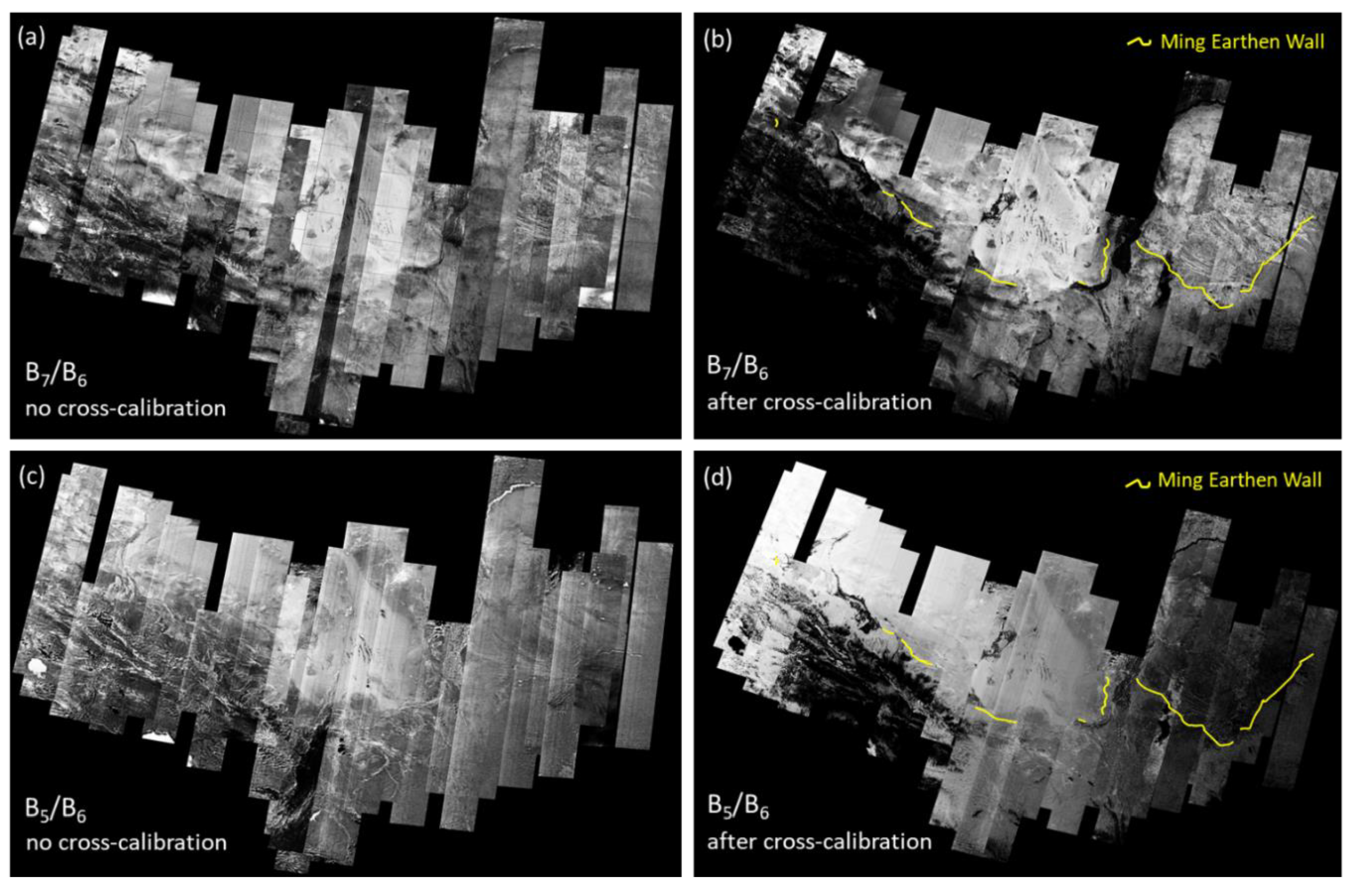
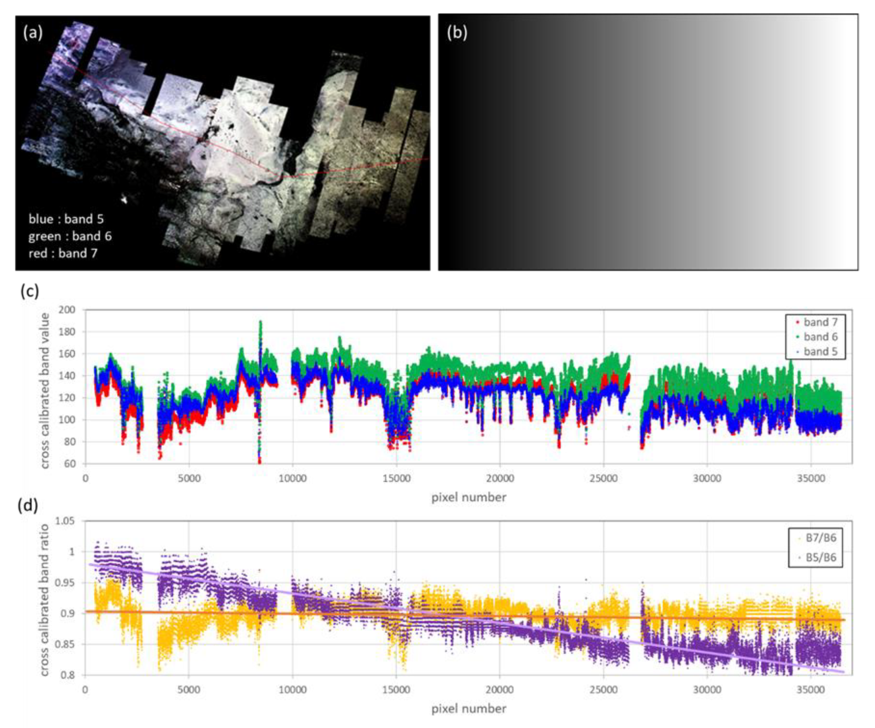
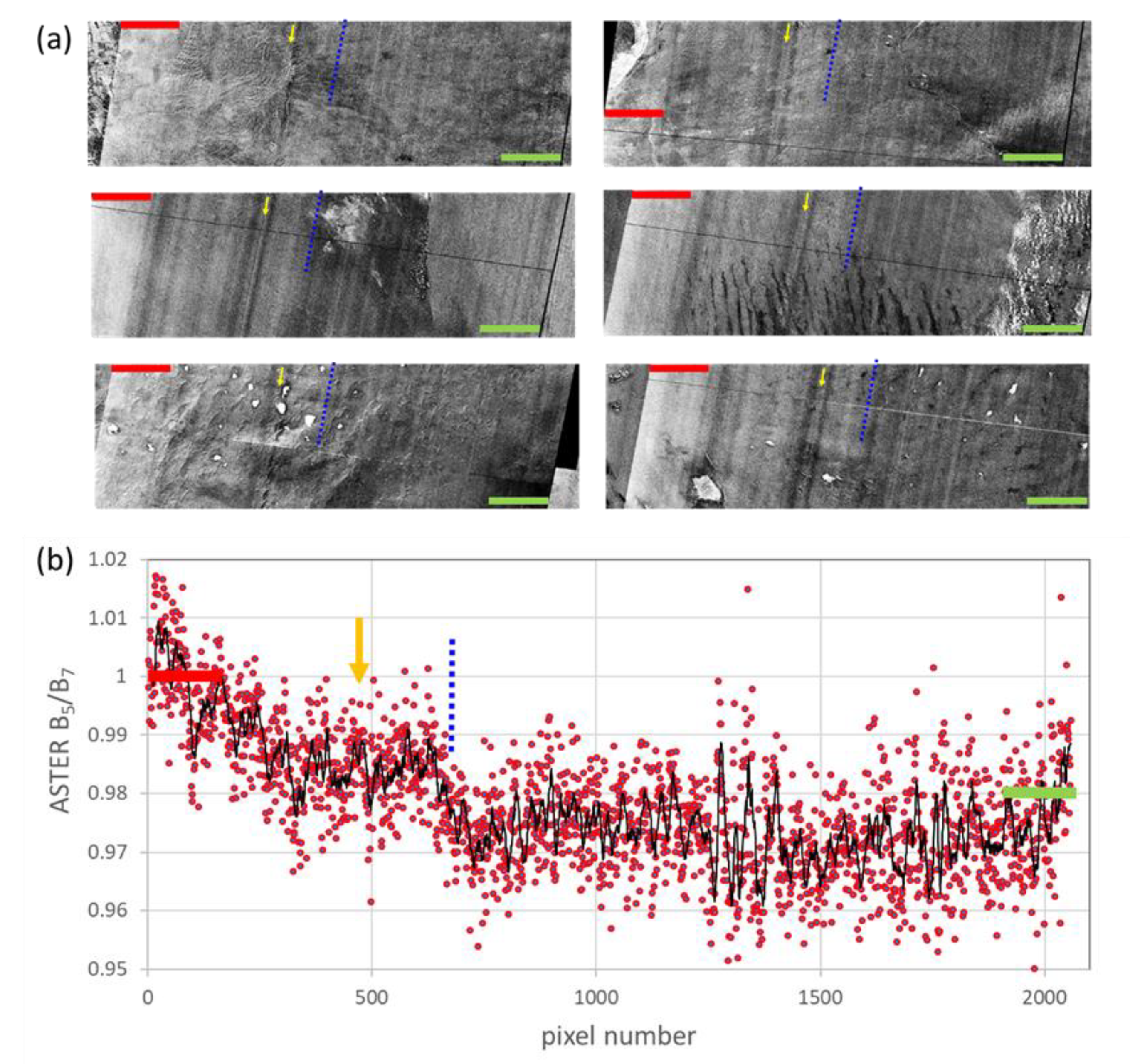
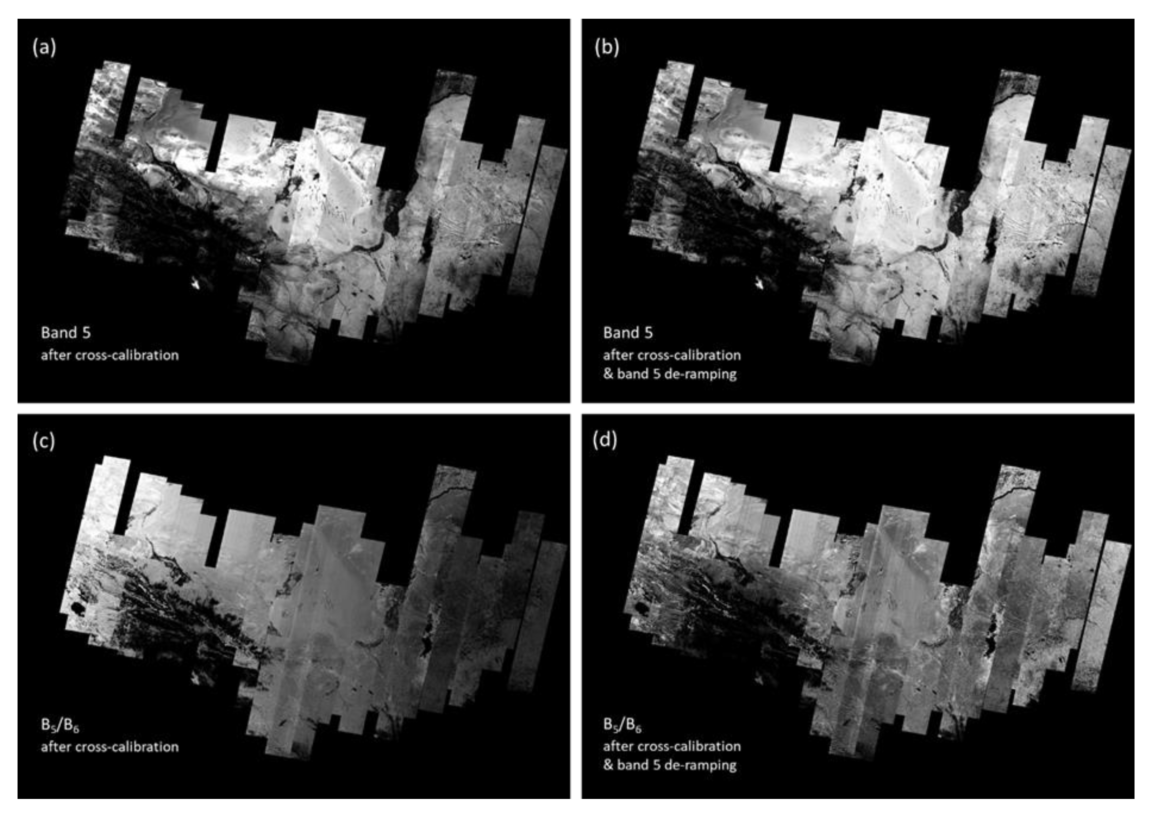
Appendix A. Systematic Detector-Array Calibration Error in ASTER Band 5

The process of generating “seamless”, compositionally-accurate mosaics from ~250 ASTER images spanning the Ming earthen wall study region required cross-calibration of 26 overlapping satellite paths. This is because, without applying this cross-calibration step to the as-received L1T ASTER data [67], subsequent band normalization techniques (e.g., band ratios) to generate compositional information would result in mismatches between adjacent images/paths, especially for the VNIR-SWIR bands (Figure A1a,c). Much of this apparent error is related to atmospheric effects, both aerosol scattering (additive effect) in the VNIR and absorption attenuation by gases such as water vapor in the SWIR (multiplicative effect). However, instrument related error is also likely, especially an additive SWIR component [60] related to uncorrected residuals of the so-called “cross-talk” effect [102].
Figure A1. (a) ASTER B7/B6 mosaic generated from L1T data, i.e., no image cross-calibration applied; (b) ASTER B7/B6 mosaic after image cross-calibration (and transformation from universal transverse Mercator (UTM) to geographic latitude-longitude); (c) ASTER B5/B6 mosaic generated from L1T data, i.e., no image cross-calibration applied; and (d) ASTER B5/B6 mosaic after image cross-calibration (and geometric transformation from UTM to geographic latitude-longitude).
Remotesensing 12 00270 g0a1
To solve these miscalibrations between images/paths, we collected VNIR-SWIR band statistics for 20–35 coincident invariant targets (or regions of interest (ROIs)) from each opposing pair of image overlaps, with each ROI comprising between 10 and 200 pixels. We then gauged whether there existed significant linear correlations for the coincident ROI band means sampled from each pair of opposing paths (which always proved to be the case). The resultant gains and offsets from these linear correlations were then used to transform (cross-calibrate) one image path to the other. This was repeated 25 times until the entire mosaic was complete. This cross-calibration method was effective for most of the VNIR-SWIR bands, as demonstrated by the B7/B6 ratio (Figure A1b). That is, previous mismatches obvious in the uncorrected L1T ratio product (Figure A1a) are absent in the cross-calibrated L1T ratio product (Figure A1b). However, ratios involving ASTER Band 5 generated a ramp effect across the mosaic, as shown by ASTER B5/B6 (Figure A1d). This ramp effect is also apparent in color composites of the cross-calibrated ASTER bands that include Band 5 (Figure A2a).
To better understand the nature of this ramp effect, we extracted pixel values from a transect across the mosaic (red line in Figure A3a) for Bands 5–7 (Figure A3c) and then generated ratios for B7/B6 and B5/B6 (Figure A2d). In contrast with the B7/B6 ratio (orange data points), which shows an overall flat trend across the transect, the B5/B6 ratio (purple data points) shows a linear slope, except for a segment of pixels from 34,000 to 37,000, which corresponds to an image path not cross-calibrated using coincident ROIs as there was no available image overlap. These results indicate that: (i) ASTER Band 5 has a systematic calibration error; and (ii) our method of using coincident ROIs across image overlaps was susceptible to this error.
Figure A2. (a) Cross-calibrated ASTER color composite of SWIR Bands R:7 G:6 B:5. A transect from which pixel values were extracted is shown by a red line. (b) A linear ramp model. (c) Pixel values of cross-calibrated Bands 5 (blue), 6 (green) and 7 (red) for the transect shown in (a). (d) The same data as in (b) but with Bands 5 and 7 each normalized with respect to Band 6. Note the linear trend in the B5/B6 ratio data (mauve line), which was used for the design of the model.
Remotesensing 12 00270 g0a2
To better understand the nature of this systematic ASTER Band 5 calibration error, a random suite of full-image-width segments from different paths and dates were sampled from the B5/B7 mosaic (Figure A3a). These normalized segments all show the same systematic noise not evident in the raw Bands 5 and 7. All segments show: (i) a broad (<200 pixels wide ) bright band on the left side of each image swath (red line); (ii) a pair of narrow (~20 pixels) dark bands (yellow arrow); and (iii) a broad shoulder (blue dotted lines). The mean B5/B7 values for six transects taken from these six images (Figure A3b) highlights this systematic line across different dates of imagery. This mean is clearly not flat across the image swath. The implication is that cross-calibration using ROIs collected from either side of a given image swath will be compromised by this systematic non-flatness. Indeed, ROIs collected from the 150 pixel-wide column on the left highlighted by the red bar will be ~2% higher than those ROIs collected from the 150 pixel-wide column on the right highlighted by the green bar. This difference drove the Band 5 miscalibration using coincident ROIs sourced from the as-received L1T data.
Figure A3. (a) A selection of six full-image-width segments from across the non-cross-calibrated ASTER B5/B7 mosaic with each showing the similar systematic column noise, including: a broad (<200 pixels wide) bright band on the left side of each image (red line); a pair of narrow (~20 pixels) dark bands (yellow arrow); and a broad shoulder (blue dotted lines). (b) Scattergram of the ASTER scene pixel number versus the mean B5/B7 values for six transects taken from (a). The 10-point moving average is shown as a black line.
Remotesensing 12 00270 g0a3
We solved this ASTER Band 5 detector array calibration issue by constructing a scaled linear-ramp model across the entire mosaic using ENVI™ software (Figure A2b), which was then used to normalize the cross-calibrated Band 5 (Figure 4a). This de-ramped Band 5 (Figure A4b) was then normalized with the cross-calibrated Band 6 to generate a B5/B6 ratio that no longer shows the ramp effect (Figure A4d). This Band 5 de-ramp process proved to be essential for all ASTER compositional products involving Band 5, such as 2200D (Figure 5a) and 2165D (Figure 6a).
Figure A4. (a) Band 5 after cross-calibration but before applying the linear ramp in (b). (b) Band 5 after cross-calibration and applying the linear ramp in (b). (c) The B5/B6 ratio after cross-calibration but before applying the linear ramp in (b). (d) The B5/B6 ratio after cross-calibration and applying the linear ramp in (b).
Remotesensing 12 00270 g0a4
In theory, this systematic ASTER Band 5 calibration error could be solved at the stage of L0 corrections where the data have not yet been rotated from their original detector array vertical column configuration, similar to that developed for satellite Hyperion push-broom sensor [103]. Implementation of an improved ASTER Band 5 detector array calibration file would solve both this east–west bias in image cross-calibration using coincident ROIs (Figure A1d) as well as remove the systematic striping observed in the current ASTER ratio products, such as those highlighted by yellow arrows in Figure 3a. Note that the image cross-calibration method used to generate the Australian ASTER mineral maps [104] was not prone to this error, as the statistics were calculated on a per-scene basis (not image overlaps) and weighted against “global” statistics.

References

  1. Lovell, J. The Great Wall: China against the World, 1000 BC-AD 2000; Grove: New York, NY, USA, 2006. [Google Scholar]
  2. Han, Z.Q. Change of the Mu Us sandy land and its relationship with the cultivation in the Ming Dynasty. Soc. Sci. China 2003, 23, 191–204. [Google Scholar]
  3. Carran, D.; Hughes, J.; Leslie, A.; Kennedy, C. A Short History of the Use of Lime as a Building Material Beyond Europe and North America. Int. J. Archit. Herit. 2012, 6, 117–146. [Google Scholar] [CrossRef]
  4. Jaquin, P.A.; Augarde, C.; Gerrard, C.M. A chronological description of the spatial development of rammed earth techniques. Int. J. Archit. Herit. Conserv. Anal. Restor. 2008, 2, 377–400. [Google Scholar] [CrossRef] [Green Version]
  5. Zewen, L.; Wilson, D.; Drege, J.-P.; Delahaye, H.; Wenbao, D.; Gernet, J. The Great Wall; McGraw-Hill: New York, NY, USA, 1984; ISBN 10: 0070707456. [Google Scholar]
  6. Shi, H.; Shao, M. Soil and water loss from the Loess Plateau in China. J. Arid Environ. 2000, 45, 9–20. [Google Scholar] [CrossRef]
  7. Li, P.; Vanapalli, S.; Li, T. Review of collapse triggering mechanism of collapsible soils due to wetting. J. Rock Mech. Geotech. Eng. 2016, 8, 256–274. [Google Scholar] [CrossRef]
  8. Porter, S.C. Chinese loess record of monsoon climate during the last glacial–interglacial cycle. Earth-Sci. Rev. 2001, 54, 115–128. [Google Scholar] [CrossRef]
  9. Küster, Y.; Hetzel, R.; Krbetschek, M.; Tao, M. Holocene loess sedimentation along the Qilian Shan (China): Significance for understanding the processes and timing of loess deposition. Quat. Sci. Rev. 2006, 25, 114–125. [Google Scholar] [CrossRef]
  10. Derbyshire, E.; Meng, X.; Kemp, R.A. Provenance, transport and characteristics of modern aeolian dust in western Gansu Province, China, and interpretation of the Quaternary loess record. J. Arid Environ. 1998, 39, 497–516. [Google Scholar] [CrossRef]
  11. Anwar, T.; Kravchinsky, V.A.; Zhang, R.; Koukhar, L.P.; Yang, L.; Yue, L. Holocene climatic evolution at the Chinese Loess Plateau: Testing sensitivity to the global warming-cooling events. J. Asian Earth Sci. 2018, 166, 223–232. [Google Scholar] [CrossRef]
  12. Lai, Z.-P.; Wintle, A.G. Locating the boundary between the Pleistocene and the Holocene in Chinese loess using luminescence. Holocene 2006, 16, 893–899. [Google Scholar] [CrossRef]
  13. Mahaney, W.C.; Hancock, R.G.V.; Zhang, L. Stratigraphy and paleosols in the Sale terrace loess section, northwest China. Catena 1990, 17, 357–367. [Google Scholar] [CrossRef]
  14. Morgan, R.P.C. Soil Erosion and Conservation; Longman Group UK Ltd.: Harlow Essex, UK, 2005; 298p. [Google Scholar]
  15. Ikari, M.J.; Kopf, A.J. Cohesive strength of clay-rich sediment. Geophys. Res. Lett. 2011, 38, L16309. [Google Scholar] [CrossRef]
  16. Trask, P.D.; Close, J.E.H. Effect of clay content on strength of soils. Coast. Eng. Proc. 1957, 1, 50. [Google Scholar] [CrossRef] [Green Version]
  17. Babu, N.; Poulose, E. Effect of lime on soil properties: A review. Int. Res. J. Eng. Technol. 2018, 5, 2395-0056. [Google Scholar]
  18. Pheng, L.S. Construction of dwellings and structures in ancient China. Struct. Surv. 2001, 19, 262–274. [Google Scholar] [CrossRef]
  19. Shao, M.; Li, L.; Wang, S.; Wang, E.; Li, Z. Deterioration mechanisms of building materials of Jiaohe ruins in China. J. Cult. Herit. 2013, 14, 38–44. [Google Scholar] [CrossRef]
  20. Pye, K. Aeolian Dust and Dust Deposits; Academic Press: London, UK, 1987. [Google Scholar]
  21. Smalley, I.J.; Krinsley, D.H. Loess deposits associated with deserts. Catena 1978, 5, 53–66. [Google Scholar] [CrossRef]
  22. Sun, J. Provenance of loess material and formation of loess deposits on the Chinese Loess Plateau. Earth Planet. Sci. Lett. 2002, 203, 845–859. [Google Scholar] [CrossRef]
  23. Pullen, A.; Kapp, P.; McCallister, A.T.; Chang, H.; Gehrels, G.E.; Garzione, C.N.; Heermance, R.V.; Ding, L. Qaidam Basin and northern Tibetan Plateau as dust sources for the Chinese Loess Plateau and paleoclimatic implications. Geology 2011, 39, 1031–1034. [Google Scholar] [CrossRef]
  24. Nie, J.; Stevens, T.; Rittner, M.; Stockli, D.; Garzanti, E.; Limonta, M.; Bird, A.; Andó, S.; Vermeesch, P.; Saylor, J.; et al. Loess Plateau storage of Northeastern Tibetan Plateau-derived Yellow River sediment. Nat. Commun. 2015, 6, 8511. [Google Scholar] [CrossRef] [Green Version]
  25. Liu, C.Q.; Masuda, A.; Okada, A.; Yabuki, S.; Fan, Z.L. Isotope geochemistry of Quaternary deposits from the arid lands in northern China. Earth Planet. Sci. Lett. 1994, 127, 25–38. [Google Scholar] [CrossRef]
  26. Sun, Y.; Tada, R.; Chen, J.; Liu, Q.; Toyoda, S.; Tani, A.; Ji, J.; Isozaki, Y. Tracing the provenance of fine-grained dust deposited on the central Chinese Loess Plateau. Geophys. Res. Lett. 2007, 35, L01804. [Google Scholar] [CrossRef]
  27. Nie, J.; Peng, W. Automated SEM–EDS heavy mineral analysis reveals no provenance shift between glacial loess and interglacial paleosol on the Chinese Loess Plateau. Aeolian Res. 2014, 13, 71–75. [Google Scholar] [CrossRef]
  28. Hu, F.; Yang, X. Geochemical and geomorphological evidence for the provenance of aeolian deposits in the Badain Jaran Desert, northwestern China. Quat. Sci. Rev. 2016, 131, 179–192. [Google Scholar] [CrossRef]
  29. Wang, X.; Cai, D.; Sun, J.; Lu, H.; Liu, W.; Qiang, M.; Cheng, H.; Che, H.; Hua, T.; Zhang, C. Contributions of modern Gobi Desert to the Badain Jaran Desert and the Chinese Loess Plateau. Sci. Rep. 2019, 9, 985. [Google Scholar] [CrossRef]
  30. Stevens, T.; Carter, A.; Watson, T.P.; Vermeesch, P.; Andò, S.; Bird, A.F.; Lu, H.; Garzanti, E.; Cottam, M.A.; Sevastjanova, I. Genetic linkage between the Yellow River, the Mu Us desert and the Chinese Loess Plateau. Quat. Sci. Rev. 2013, 78, 355–368. [Google Scholar] [CrossRef]
  31. Bird, A.; Stevens, T.; Rittner, M.; Vermeesch, P.; Carter, A.; Andò, S.; Garzanti, E.; Lu, H.; Nie, J.; Zeng, L.; et al. Quaternary dust source variation across the Chinese Loess Plateau. Palaeogeogr. Palaeoclimatol. Palaeoecol. 2015, 435, 254–264. [Google Scholar] [CrossRef]
  32. Wang, F.; Sun, D.; Chen, F.; Bloemendal, J.; Guo, F.; Li, Z.; Zhang, Y.; Li, B.; Wang, X. Formation and evolution of the Badain Jaran Desert, North China, as revealed by a drill core from the desert centre and by geological survey. Palaeogeogr. Palaeoclimatol. Palaeoecol. 2015, 426, 139–158. [Google Scholar] [CrossRef]
  33. Shi, Z.; Liu, X. Distinguishing the provenance of fine-grained eolian dust over the Chinese Loess Plateau from a modelling perspective. Tellus 2011, 63, 959–970. [Google Scholar] [CrossRef]
  34. Huang, C.Q.; Zhao, W.; Li, F.Y.; Tan, W.F.; Wang, M.K. Mineralogical and pedogenetic evidence for palaeoenvironmental variations during the Holocene on the Loess Plateau, China. Catena 2012, 96, 49–56. [Google Scholar] [CrossRef]
  35. Ding, Z.L.; Sun, J.M.; Yang, S.L.; Liu, T.S. Geochemistry of the Pliocene red clay formation in the Chinese Loess Plateau and implications for its origin, source provenance and paleoclimate change. Geochim. Cosmochim. Acta 2001, 65, 901–913. [Google Scholar] [CrossRef]
  36. Zhao, W.; Liu, L.; Chen, J.; Ji, J. Geochemical characterization of major elements in desert sediments and implications for the Chinese loess source. Sci. China Earth Sci. 2019, 62, 1428–1440. [Google Scholar] [CrossRef]
  37. Licht, A.; Pullen, A.; Kapp, P.; Abell, J.; Giesler, N. Eolian cannibalism: Reworked loess and fluvial sediment as the main sources of the Chinese Loess Plateau. Geol. Soc. Am. Bull. 2016, 128, 944–956. [Google Scholar] [CrossRef] [Green Version]
  38. Sun, J.; Ding, Z.; Xi, X.; Sun, M.; Windley, B.F. Detrital zircon evidence for the ternary sources of the Chinese Loess Plateau. J. Asian Earth Sci. 2018, 155, 21–34. [Google Scholar] [CrossRef]
  39. Lü, T.; Sun, J. Luminescence sensitivities of quartz grains from eolian deposits in northern China and their implications for provenance. Quat. Res. 2011, 76, 181–189. [Google Scholar] [CrossRef]
  40. Sun, Y.; Chen, H.; Tada, R.; Weiss, D.; Lin, M.; Toyoda, S.; Yan, Y.; Isozaki, Y. ESR signal intensity and crystallinity of quartz from Gobi and sandy deserts in East Asia and implication for tracing Asian dust provenance. Geochem. Geophys. Geosyst. 2013, 14, 2615–2627. [Google Scholar] [CrossRef]
  41. Ma, L.; Sun, Y.; Tada, R.; Yan, Y.; Chen, H.; Lin, M.; Nagashima, K. Provenance fluctuations of aeolian deposits on the Chinese Loess Plateau since the Miocene. Aeolian Res. 2015, 18, 1–9. [Google Scholar] [CrossRef]
  42. Yan, Y.; Ma, L.; Sun, Y. Tectonic and climatic controls on provenance changes of fine-grained dust on the Chinese Loess Plateau since the late Oligocene. Geochim. Cosmochim. Acta 2017, 200, 110–122. [Google Scholar] [CrossRef]
  43. Chen, Z.; Li, G. Evolving sources of eolian detritus on the Chinese Loess Plateau since early Miocene: Tectonic and climatic controls. Earth Planet. Sci. Lett. 2013, 371–372, 220–225. [Google Scholar] [CrossRef]
  44. Zhang, W.; Chen, J.; Li, G. Shifting material source of Chinese loess since ~2.7 Ma reflected by Sr isotopic composition. Sci. Rep. 2015, 5, 10235. [Google Scholar] [CrossRef] [Green Version]
  45. Maher, B.A.; Mutch, T.J.; Cunningham, D. Magnetic and geochemical characteristics of Gobi Desert surface sediments: Implications for provenance of the Chinese Loess Plateau. Geology 2009, 37, 279–282. [Google Scholar] [CrossRef]
  46. Zhao, L.; Ji, J.; Chen, J.; Liu, L.; Chen, Y.; Balsam, W. Variations of illite/chlorite ratio in Chinese loess sections during the last glacial and interglacial cycle: Implications for monsoon reconstruction. Geophys. Res. Lett. 2005, 32, L20718. [Google Scholar] [CrossRef]
  47. Jeong, G.Y.; Hillier, S.; Kemp, R.A. Quantitative bulk and single-particle mineralogy of a thick Chinese loess–paleosol section: Implications for loess provenance and weathering. Quat. Sci. Rev. 2008, 27, 1271–1287. [Google Scholar] [CrossRef]
  48. Jeong, G.Y.; Hillier, S.; Kemp, R.A. Changes in mineralogy of loess–paleosol sections across the Chinese Loess Plateau. Quat. Res. 2011, 75, 245–255. [Google Scholar] [CrossRef]
  49. Formenti, P.; Schutz, L.; Balkanski, Y.; Desboeufs, K.; Elbert, M.; Kandler, K.; Petzold, A.; Scheuvens, D.; Weinbruch, S.; Zhang, D. Recent progress in understanding physical and chemical properties of African and Asian mineral dust. Atmos. Chem. Phys. 2011, 11, 8231–8256. [Google Scholar] [CrossRef] [Green Version]
  50. Schaetzl, R.J.; Bettis, E.A., III; Crouvi, O.; Fitzsimmons, K.E.; Grimley, D.A.; Hambacf, U.; Lehmkuhl, F.; Marković, S.B.; Mason, J.A.; Owczarek, P.; et al. Approaches and challenges to the study of loess—Introduction to the LoessFest Special Issue. Quat. Res. 2018, 89, 563–618. [Google Scholar] [CrossRef] [Green Version]
  51. McCuaig, C.T.; Beresford, S.; Hronsky, J. Translating the mineral systems approach into an effective exploration targeting system. Ore Geol. Rev. 2010, 38, 128–138. [Google Scholar] [CrossRef]
  52. Cudahy, T.J. Mineral Mapping for Exploration: An Australian Journey of Evolving Spectral Sensing Technologies and Industry Collaboration. Geosciences 2016, 6, 52. [Google Scholar] [CrossRef] [Green Version]
  53. Wyborn, L.A.; Heinrich, C.A.; Jacques, A.L. Australian Proterozoic mineral systems: Essential ingredients and mappable criteria. In Proceedings of the AusIMM Annual Conference Proceedings, Darwin, Australia, 5–9 August 1994; pp. 109–115. [Google Scholar]
  54. Smalley, I.; Marshall, J.; Fitzsimmons, K.; Whalley, W.B.; Ngambi, S. Desert loess: A selection of relevant topics. Geologos 2019, 25, 91–102. [Google Scholar] [CrossRef] [Green Version]
  55. Yamaguchi, Y.; Kahle, A.B.; Tsu, H.; Kawakami, T.; Pniel, M. Overview of Advanced Space-borne Thermal Emission and Reflection Radio. meter (ASTER). IEEE Trans. Geosci. Remote Sens. 1998, 36, 1062–1071. [Google Scholar] [CrossRef] [Green Version]
  56. Abrams, M.; Tsu, H.; Hulley, G.; Iwao, K.; Pieri, D.; Cudahy, T.J.; Kargel, J. The Advanced Spaceborne Thermal Emission and Reflection Radiometer (ASTER) after fifteen years: Review of global products. Int. J. Appl. Earth Obs. Geoinf. 2015, 38, 292–301. [Google Scholar] [CrossRef]
  57. Clark, R.N. Chapter 1: Spectroscopy of Rocks and Minerals, and Principles of Spectroscopy. In Manual of Remote Sensing; Rencz, A.N., Ed.; John Wiley and Sons: New York, NY, USA, 1999; Volume 3, pp. 3–58. [Google Scholar]
  58. Cudahy, T.J. Australian ASTER Geoscience Product Notes; CSIRO Report, EP-30-07-12-44; Commonwealth Scientific and Industrial Research Organisation (CSIRO): Canberra, Australia, 2012. Available online: https://data.csiro.au/dap/landingpage?pid=csiro%3A6182 (accessed on 28 September 2019).
  59. Rowan, L.C.; Mars, J.C. Lithologic mapping in the Mountain Pass, California area using Advanced Spaceborne Thermal Emission and Reflection Radiometer (ASTER) data. Remote Sens. Environ. 2003, 84, 350–366. [Google Scholar] [CrossRef]
  60. Hewson, R.D.; Cudahy, T.J.; Mizukiko, S.; Mauger, A.L. Seamless geological map generation using ASTER in the Broken Hill Curnamona Province of Australia. Remote Sens. Environ. 2005, 99, 159–172. [Google Scholar] [CrossRef]
  61. Agisoft Metashape Software. Available online: https://www.agisoft.com (accessed on 7 December 2019).
  62. Raven, M.D.; Self, P.G. Xplot user manual, manipulation of powder X-ray diffraction data. In CSIRO Division of Soils Technical Memorandum; 30/1988; CSIRO: Canberra, Australia, 1988; 25p. [Google Scholar]
  63. ICDD Mineral Standards Library. Available online: http://www.icdd.com (accessed on 30 October 2019).
  64. Analytical Spectral Devices (ASD) FieldSpec Pro Spectrometer. Available online: https://www.malvernpanalytical.com/en/products/product-range/asd-range (accessed on 30 October 2019).
  65. Spectralon Panel. Available online: http://www.labsphere.com (accessed on 30 October 2019).
  66. Korb, A.R.; Dybwad, P.; Wadsworth, W.; Salisbury, J.W. Portable Fourier transform infrared spectroradiometer for field measurements of radiance and emissivity. Appl. Opt. 1996, 35, 1679–1692. [Google Scholar] [CrossRef] [PubMed] [Green Version]
  67. Earthdata Web Portal. Available online: https://search.earthdata.nasa.gov/search (accessed on 30 October 2019).
  68. Ninomiya, Y.; Fu, B.; Cudahy, T.J. Detecting lithology with Advanced Spaceborne Thermal Emission and Reflectance Radiometer (ASTER) multispectral thermal infrared “radiance-at-sensor” data. Remote Sens. Environ. 2005, 99, 127–139. [Google Scholar] [CrossRef]
  69. Shi, P.; Fu, B.; Cudahy, T.J.; Guo, Q.; Xu, H.; Chen, X.; Ma, Y.; Xue, G. Desertification monitoring using the ASTER global emissivity dataset. In Proceedings of the 2017 IEEE International Geoscience and Remote Sensing Symposium (IGARSS), Fort Worth, TX, USA, 23–28 July 2017; pp. 4501–4504. [Google Scholar] [CrossRef]
  70. Cudahy, T.J.; Jones, M.; Lisitsin, V.; Caccetta, M.; Collings, S.; Bateman, R. 3D Mineral Mapping of Queensland-Version 2 ASTER and Related Geoscience Products; CSIRO Mineral Resources; EP1767; 18p, Available online: https://publications.csiro.au/rpr/download?pid=csiro:EP17697&dsid=DS3 (accessed on 6 October 2019).
  71. Ninomiya, Y. Quantitative estimation of SiO2 content in igneous rocks using thermal infrared spectra with a neural network approach. IEEE Trans. Geosci. Remote Sens. 1995, 33, 684–691. [Google Scholar] [CrossRef]
  72. Hunt, G.R.; Vincent, R.K. The behaviour of spectral features in the infrared emission from particulate surfaces of various grain sizes. J. Geophys. Res. 1968, 73, 6039–6046. [Google Scholar] [CrossRef]
  73. Salisbury, J.W.; Walter, L.S. Thermal infrared (2.5–13.5 m) spectroscopic remote sensing of igneous rock types on particulate planetary surfaces. J. Geophys. Res. 1989, 94, 9192–9202. [Google Scholar] [CrossRef]
  74. Clark, R.N. Spectral properties of mixtures of montmorillonite and dark carbon grains: Implications for remote sensing minerals containing chemically and physically absorbed water. J. Geophys. Res. 1983, 88, 10635–10644. [Google Scholar] [CrossRef]
  75. Haest, M.; Cudahy, T.; Laukamp, C.; Gregory, S. Quantitative mineralogy from visible to shortwave infrared spectroscopic data—I. Validation of mineral abundance and composition products of the Rocklea Dome channel iron deposit in Western Australia. Econ. Geol. 2012, 107, 209–228. [Google Scholar] [CrossRef]
  76. Haest, M.; Cudahy, T.; Laukamp, C.; Gregory, S. Quantitative mineralogy from visible to shortwave infrared spectroscopic data—II. 3D mineralogical characterisation of the Rocklea Dome channel iron deposit, Western Australia. Econ. Geol. 2012, 107, 229–249. [Google Scholar] [CrossRef]
  77. Rodger, A.R.; Cudahy, T.J. Vegetation Corrected Continuum Depths at 2.20 μm: An Approach for Hyperspectral Sensors. Remote Sens. Environ. 2009, 113, 2243–2257. [Google Scholar] [CrossRef]
  78. Haest, M.; Cudahy, T.J.; Rodger, A.; Laukamp, C.; Martens, C.; Caccetta, M. Unmixing vegetation from airborne visible-near to shortwave infrared spectroscopy-based mineral maps over the Rocklea Dome (Western Australia), with a focus on iron rich palaeochannels. Remote Sens. Environ. 2013, 129, 17–31. [Google Scholar] [CrossRef]
  79. Du, Y.; Chen, W.; Cui, K.; Gong, S.; Pu, T.; Fu, X. A Model characterizing deterioration at earthen sites of the Ming Great Wall in Qinghai Province, China. Soil Mech. Found. Eng. 2017, 53, 426–434. [Google Scholar] [CrossRef]
  80. Allen, J.R. Physical Processes of Sedimentation; Earth Science Series 1; Sutton, J., Watson, J.W., Eds.; Unwin University Books: London, UK, 1970. [Google Scholar]
  81. Hook, S.J.; Dmochowski, J.E.; Howard, K.A.; Rowan, L.C.; Karlstrom, K.E.; Stock, J.M. Mapping variations in weight percent silica measured from multispectral thermal infrared imagery—Examples from the Hiller Mountains, Nevada USA and Tres Virgenes-La Reforma, Baja California Sur, Mexico. Remote Sens. Environ. 2005, 95, 273–289. [Google Scholar] [CrossRef]
  82. Pan, P.; Pang, H.; Zhang, D.; Guan, Q.; Wang, L.; Li, F.; Guan, W.; Cai, A.; Sun, X. Sediment grain-size characteristics and its source implication in the Ningxia–Inner Mongolia sections on the upper reaches of the Yellow River. Geomorphology 2015, 246, 255–262. [Google Scholar] [CrossRef]
  83. Pan, B.; Pang, H.; Gao, H.; Garzanti, E.; Zou, Y.; Liu, X.; Li, F.; Jia, Y. Heavy-mineral analysis and provenance of Yellow River sediments around the China Loess Plateau. J. Asian Earth Sci. 2016, 127, 1–11. [Google Scholar] [CrossRef] [Green Version]
  84. Jia, X.; Li, Y.; Wang, H. Bed sediment particle size characteristics and its sources implication in the desert reach of the Yellow River. Environ. Earth Sci. 2016, 75, 950. [Google Scholar] [CrossRef]
  85. Kalm, V.E.; Rutter, N.W.; Rokosh, C.D. Clay minerals and their paleoenvironmental interpretation in the Baoji loess section, Southern Loess Plateau, China. Catena 1996, 27, 49–61. [Google Scholar] [CrossRef]
  86. Bell, F.G. Lime stabilization of clay minerals and soils. Eng. Geol. 1996, 42, 223–237. [Google Scholar] [CrossRef]
  87. Koporulin, V.I. Formation of laumontite in sedimentary rocks: A case study of sedimentary sequences in Russia. Lithol. Miner. Resour. 2013, 48, 122–137. [Google Scholar] [CrossRef]
  88. Eden, D.N.; Qizhong, W.; Hunt, J.L.; Whitton, J.S. Mineralogical and geochemical trends across the Loess Plateau, North China. Catena 1994, 21, 73–90. [Google Scholar] [CrossRef]
  89. Begét, J.E.; Keskinen, M.; Severin, K. Mineral particles from Asia found in volcanic loess on the island of Hawaii. Sediment. Geol. 1993, 84, 189–197. [Google Scholar] [CrossRef]
  90. Yao, Z.; Shi, X.; Qiao, S.; Liu, Q.; Kandasamy, S.; Liu, J.; Liu, Y.; Liu, J.; Fang, X.; Gao, J.; et al. Persistent effects of the Yellow River on the Chinese marginal seas began at least ~880 ka ago. Sci. Rep. 2017, 7, 2827. [Google Scholar] [CrossRef] [Green Version]
  91. Harder, H. Illite mineral synthesis at surface temperatures. Chem. Geol. 1974, 14, 241–253. [Google Scholar] [CrossRef]
  92. Laurent, B.; Marticorena, B.; Bergametti, G.; Mei, F. Modeling mineral dust emissions from Chinese and Mongolian deserts. Glob. Planet. Chang. 2006, 52, 121–141. [Google Scholar] [CrossRef]
  93. Wang, Q.; Zhuang, G.; Huang, K.; Liu, T.; Lin, Y.; Deng, C.; Fu, Q.; Fub, J.S.; Chen, J.; Zhang, W.; et al. Evolution of particulate sulfate and nitrate along the Asian dust pathway: Secondary transformation and primary pollutants via long-range transport. Atmos. Res. 2016, 169, 86–95. [Google Scholar] [CrossRef]
  94. Pu, T.; Chen, W.; Du, Y.; Li, W.; Su, N. Snowfall-related deterioration behavior of the Ming Great Wall in the eastern Qinghai-Tibet. Nat. Hazards 2016, 84, 1539–1550. [Google Scholar] [CrossRef]
  95. Green, R.; Mahowald, N.; Thompson, D.; Clark, R.; Ehlmann, B.; Ginoux, P.; Kalashnikova, O.; Miller, R.; Okin, G.; Painter, P.; et al. The Earth Surface Mineral Dust Source Investigation Planned for the International Space Station. Geophys. Res. Abstr. 2019, 21, EGU2019-10660. [Google Scholar]
  96. HISUI. Available online: https://hyspiri.jpl.nasa.gov/downloads/2018_Workshop/day3/14_1808_HISUI_Matsunaga_04b.pdf (accessed on 4 July 2019).
  97. ECOSTRESS. Available online: https://ecostress.jpl.nasa.gov/news (accessed on 4 July 2019).
  98. Tollefson, J.; Gilbert, N. Rio report card. Nature 2012, 486, 20–23. [Google Scholar] [CrossRef]
  99. Sommer, S.; Zucca, C.; Grainger, A.; Cherlet, M.; Zougmore, R.; Sokona, Y.; Hill, J.; Della Peruta, R.; Roehrig, J.; Wang, G. Application of indicator systems for monitoring and assessment of desertification from National to Global scale. Land Degrad. Dev. 2012, 22, 184–197. [Google Scholar] [CrossRef]
  100. Vogt, J.V.; Safriel, U.; von Maltitz, G.; Sokona, Y.; Zougmore, R.; Bastin, G.; Hill, J. Monitoring and assessment of land degradation and desertification: Towards new conceptual and integrated approaches. Land Degrad. Dev. 2011, 22, 150–165. [Google Scholar] [CrossRef]
  101. Cudahy, T.; Caccetta, M.; Thomas, M.; Hewson, R.; Abrams, M.; Kato, M.; Kashimura, O.; Ninomiya, Y.; Yamaguchi, Y.; Collings, S.; et al. Satellite-derived mineral mapping and monitoring of weathering, deposition and erosion. Sci. Rep. 2016, 6, 23702. [Google Scholar] [CrossRef] [PubMed]
  102. Iwasaki, A.; Tonooka, H. Validation of a crosstalk correction algorithm for ASTER/SWIR. IEEE Trans. Geosci. Remote Sens. 2005, 43, 2747–2751. [Google Scholar] [CrossRef]
  103. Cudahy, T.J.; Rodger, A.R.; Barry, P.S.; Mason, P.; Quigley, M.A.; Folkman, M.A.; Pearlman, J. Assessment of the stability of the Hyperion SWIR module for hyperspectral mineral mapping using multi-date images from Mount Fitton, Australia. In Proceedings of the IEEE 2002 International Conference on Geoscience and Remote Sensing, Toronto, ON, Canada, 24–28 June 2002. [Google Scholar]
  104. Caccetta, M.; Collings, S.; Cudahy, T.J. A calibration method for continental scale mapping using ASTER imagery. Remote Sens. Environ. 2012, 139, 306–317. [Google Scholar] [CrossRef]
Figure 1. (a) Satellite ASTER false-color mosaic (Band 3: red; Band 2: green; Band 1: blue) spanning the Ordos Plateau and Hexi Corridor from Shenmu in the east to Jiayuguan in the west and including approximately 1200 km of the earthen Ming Great Wall (yellow line). The geological blocks, mountains, deserts, rivers, loess extent, thickness of the late-Pleistocene Malan loess unit [8], towns/cities, and field sample sites are also shown. (be) Oblique views of rendered digital elevation models of selected field sites generated from drone natural color imagery. The nature of local surface materials is indicated as well as several features of the wall.
Remotesensing 12 00270 g001
Figure 2. Field site photos and data. (a) Twenty-centimeter-wide layering of the Ming earthen wall (cyan arrows) at Site 48 (38°19.33′N; 101°58.25′E. (b) Abundant white clay-carbonate fragments within “hangtu” construction layers at Site 28 (37°56.29′N; 107°13.49′E). (c) A recently exposed cutting <1 km from Site 28 exposing a ~1 m thick surface layer of loess developed over an eroded red and white horizontal layered clay-rich paleosol with white clay-carbonate fragments. (d) South-side view of the well-preserved earthen wall at Site 48 (38°19.33′N; 101°58.25′E). Preferentially eroding “hangtu” layers are shown by green arrows while sub-vertical rills are shown by yellow arrows. Field sampling points for pXRF and ASD measurements are numbered (#). (e) Close-up view at Site 48 showing isolated, sub-rounded grey siltstone pebbles and cobbles in a beige colored loess matrix. (f) A road cutting along the Shandan section (38°27.40′N; 101°27.53′E) showing a ~1 m thick surface layer of loess developed over grey, sub-rounded, siltstone pebbles, and cobbles similar to those evident in (e). (g) A table of field pXRF chemistry and ASD gypsum information of selected sample points (#) in (d,i). (h) Preferential erosion along multiple “hangtu” layers at Site 33 (38°16.34′N; 106°32.18′E). (i) Recent collapse of the earthen wall at Site 38 (37°57.34′N; 105°47.78′E) related to undercutting along a ~50 cm wide erosional zone (#7) rich in halite. (j) Visual classification of the earthen wall’s erosional status where: 1 = little remaining of the original wall above the exposed land surface; and 5 = well-preserved wall, including the remnants of battlements. The magenta box highlights the well-preserved Shandan section.
Remotesensing 12 00270 g002
Figure 3. Laboratory analyses of field samples. (a) Scattergram of the mean (n = 43) and standard deviation (STD) for each of the 19 particle size bins. Four populations are highlighted: 0.1–3.0 µm (blue box) with a peak at 2 µm and called “clay”; 3–20 µm (green box) with a peak at 10 µm and called “fine-silt”; 20–50 (yellow box) with a peak at 50 µm called “coarse silt”; and 50–2000 µm (red box) and called “sand”. (b) Scattergram of the west-to-east pattern in mean particle size content for each of the four groupings. (c) Scattergram of the west-to-east spatial trend in the combined clay and fine-silt fractions (<20 µm) normalized with respect to sand (>50 µm) content. (d) Scattergram of the particle-size bin versus the fitted linear correlation (R2, n = 43) between a sample site’s given particle size content and its distance to one of three potential source areas, i.e., sand dunes, Tengger Desert evaporative lakes, and Qilian Shan alluvial fans. (e) Scattergram of the west-to-east pattern for field site portable XRF measurements of Si/(Si + Al + Fe) for both wall and background samples. (f) Scattergram of the west-to-east pattern of field site portable XRF measurements of Fe, Ca, Mg, S, and Cl of wall samples. (g) Scattergram of the west-to-east spatial trend of field site portable XRF measurements of Fe, Ca, Mg, S, and Cl of background samples. (h) East-to-west pattern of minerals detected using XRD. A magenta box highlights the well-preserved “Shandan” wall section. (i) Selected field ASD spectra. Diagnostic mineral absorptions are highlighted as well as the ASTER band-passes.
Remotesensing 12 00270 g003
Figure 4. (a) ASTER SI3 base-map depicting the proportion of quartz sand (warm colors) to clay (cool colors) material overlain with a threshold mask of the ASTER Gypsum Index (white). (b) Scattergram of the west-to-east spatial trend of satellite ASTER SI3 responses collected from three (north, south, and centered over the wall) ROIs (~50 pixels each) of the field sites. (c) Scattergram of the west-to-east spatial trend of field SI3 responses of wall samples only. A magenta box highlights the well-preserved “Shandan” wall section.
Remotesensing 12 00270 g004
Figure 5. (a) Satellite ASTER 2200D index base-map depicting the amount of Al-bearing minerals (i.e., muscovite/illite, kaolinite) with greater abundances in warmer tones. (b) Scattergram of the west-to-east spatial trend of satellite ASTER 2200D responses of ROIs collected from three (north, south, and centered over the wall) ROIs (~50 pixels each) of the field sites. (c) Scattergram of the west-to-east spatial trend of field 2200D responses of both wall (filled red triangles) and background (open red triangles) samples. Fifth-order polynomials are fitted to the satellite and background field sample data. A magenta box highlights the well-preserved “Shandan” wall section.
Remotesensing 12 00270 g005
Figure 6. (a) Satellite ASTER 2165D index base-map depicting the proportion of kaolin (warmer tones) versus white mica (cooler tones). (b) Scattergram of the west-to-east spatial trend of satellite ASTER 2165D ROI responses. (c) Scattergram of the west-to-east spatial trend of field 2165D responses of both wall (filled red circles) and background (open red circles) samples. These are underlain by laboratory XRD results of the 7.169 Å kaolinite peak height (green boxes) for selected wall samples. A magenta box highlights the well-preserved “Shandan” wall section.
Remotesensing 12 00270 g006
Figure 7. (a) Satellite ASTER 2330D mosaic, which is sensitive to the content of chlorite. (b) Scattergram of the west-to-east spatial trend of satellite ASTER 2330D ROI responses. (c) Scattergram of the west-to-east spatial trend of field 2330D responses of both wall (filled red circles) and background (open red circles) samples. These are plotted with laboratory XRD results of the 14.1 Å chlorite peak height (green boxes) for selected wall samples. A magenta box marks the well-preserved “Shandan” wall section.
Remotesensing 12 00270 g007
Table 1. A mineral-based “loess system” sediment transport model using ASTER satellite imagery.
Sand Sub-SystemClay and Fine Silt Sub-System
Essential components(i) quartz(ii) white mica (muscovite and/or illite)
(iii) chlorite
(iv) kaolinite
(v) gypsum
ASTER mappable criteria(i) ASTER SI3 index(ii) ASTER 2200D and 2165D indices
(iii) ASTER 2200D and 2165D indices
(iv) ASTER 2300D index
(v) ASTER SI3 index
Particle size(i) sand(ii)–(iv) fine-silt to clay
(v) fine silt (?)
Primary source(i) Mesozoic and Cainozoic sedimentary rocks exposed in the Gobi Desert(ii) pre-Mesozoic metamorphic rocks of the Alashan Block
(iii) pre-Mesozoic metamorphic rocks of the Alashan Block
(iv) Devonian molasse exposed in the Qilian Shan
(v) evaporative lakes of the Tengger Desert
Transport mechanisms• aeolian saltation by westerly winds west of the Yellow River • aeolian long-term suspension by westerly to northwesterly winds
• Fluvial erosion alongside the Tengger and Hobq Deserts and deposition alongside the Hobq Desert.
• aeolian saltation by northerly winds east of the Yellow River
Detectable gradient size• <200 km• >500 km
Pathway constraints• connected (downslope or flat) lowlands• topography <2000 m elevation above background
• topography <100 m elevation above background
Sediment traps/reservoirs• eastern Badain Jaran Desert (topographic upslope)(ii) and (iii) eastern Badain Jaran and Tengger Deserts
• Hobq Desert (Yellow River braided system bedload deposition)(iv) alluvial fans off the Qilian Shan
• Mu Us Desert (topographic upslope)(ii)–(v) low energy, long-term suspension dust fallout areas, topographically shielded from saltation flow of sand

