Abstract
High frequency surface wave radar (HFSWR) plays an important role in marine surveillance on account of its ability to provide wide-range early warning detection. However, vessel target track breakages are common in large-scale marine monitoring, which limits the continuous tracking ability of HFSWR. The following are the possible reasons for track fracture: highly maneuverable vessels, dense channels, target occlusion, strong clutter/interference, long sampling intervals, and low detection probabilities. To solve this problem, we propose a long-term continuous tracking method for multiple targets with stereoscopic HFSWR based on an interacting multiple model extended Kalman filter (IMMEKF) combined with an extreme learning machine (ELM). When the trajectory obtained by IMMEKF breaks, a new section of the track will start on the basis of the observation data. For multiple-target tracking, a number of broken tracks can be obtained by IMMEKF tracking. Then the ELM classifies the segments from the same vessel by extracting different features including average velocity, average curvature, ratio of the arc length to the chord length, and wavelet coefficient. Both the simulation and the field experiment results validate the method presented here, showing that this method can achieve long-term continuous tracking for multiple vessels, with an average correct track segment association rate of over 91.2%, which is better than the tracking performance of conventional algorithms, especially when the vessels are in dense channels and strong clutter/interference area.
1. Introduction
High-frequency surface wave radar (HFSWR) has become the primary technical means for maritime-state monitoring [1,2]. However, track breakages frequently occur in large-scale marine surveillance due to highly maneuverable targets, dense channels, target occlusion, strong clutter/interference, long sampling intervals, and low detection probabilities, which substantially degrade the overall tracking performance and adversely affect situation assessment [3,4]. Hence, continuous tracking of vessels is one of the key problems to be solved in the field of target tracking in marine surveillance.
At present, algorithm research studies for long-term vessel tracking mainly center on segment association, which can be divided into two categories: one is based on statistics [5,6,7,8,9]; the other is based on fuzzy mathematics [10,11,12,13]. The former takes the difference of the state estimation as the statistic, establishes the hypothesis, and then uses the given probability to accept or reject the hypothesis to determine whether the track is associated or not. The latter selects the membership degree of association, and calculates the membership value of two tracks to determine whether the track is associated or not. Bar-Shalom et al. [5] applied the fixed distance metric in the weighted statistical method. Yeom et al. [6] presented a track segment association algorithm on the basis of discrete optimization. Zhang et al. [7] stitched broken tracks by using an interacting multiple model (IMM) estimator. Aybars et al. [8] calculated an association cost in order to associate tracks on the basis of Mahalanobis distance. Zhu et al. [9] proposed a mixed integer nonlinear programming (MINLP) model in the maximum likelihood rule. Ashraf et al. [10] presented a fuzzy correlation approach on the basis of the fuzzy clustering means algorithm. Stubberud et al. [11] proposed a straightforward fuzzy-logic-based association method based on the chi 2 metric. Shao et al. [12] used fuzzy k-nearest neighbors and fuzzy C-means clustering to achieve track segment association. Hong et al. [13] presented a track segment association algorithm by calculating the fuzzy membership matrix and clustering methodology. All of these methods compare the distances of track segments point by point without considering the relevance of the track segments’ features, which can cause invalid track association when a vessel is in a complex situation, such as in a dense channel or strong clutter interference region.
These track segment association (TSA) algorithms are feasible in theory, however, the backward prediction error of the present track is often large due to the noise of the system and measurement, which results in poor accuracy of association. Even worse, the performance of TSA algorithms drops suddenly due to track crossing and bifurcation when affected by surrounding large vessels or strong clutters. In order to solve the track breakage problem effectively and track targets steadily and continuously, we consider combining the conventional tracking algorithm with the machine learning method, which can achieve track segment association through studying the training dataset. The back propagation (BP) network has a strong nonlinear mapping ability, although it easily becomes trapped in local minimums during its training, which limits the stability and accuracy of classification [14,15]. Although the support vector machine (SVM) is able to avoid a local optimal solution, it has some shortcomings, such as training slowly and having a low efficiency [16,17]. The extreme learning machine (ELM) is a single hidden layer neural network with low computational complexity and good general performance [18]. Compared with the traditional neural network, ELM can randomly initialize the input weight and offset without adjusting during the training process, which make it simple and fast with the guarantee of accuracy [19]. Moreover, the ELM is more suited to handle small sample classification problems than deep learning [20,21].
We propose a long-term continuous tracking method based on an interacting multiple model extended Kalman filter (IMMEKF) combined with an extreme learning machine (ELM). When using the IMMEKF tracking method alone, we can determine only the intermittent track segments. Long-term continuous tracking is achieved when the ELM is combined with this method. In order to sufficiently reflect the track segment features, we associate the tracks on the basis of features extracted from track segments rather than comparing the distances of track segments point by point. Moreover, we present a new scheme to solve the problem of track segment association using an ELM network. The method decides whether the present track segment is associated with the former tracks through the ELM network, whose feature vectors in the training set are extracted from the track segments obtained by the IMMEKF. Hence, the long-term continuous tracking of multiple targets can be achieved via the cooperation between the IMMEKF and the ELM. Both the simulation and the field experiment results show that the proposed method has better tracking performance than conventional algorithms.
This paper is organized as follows. In Section 2, we briefly introduce the stereoscopic HFSWR station and the system model of the vessel target. In Section 3, we propose the long-term continuous tracking method with stereoscopic HFSWR based on IMMEKF combined with ELM. Furthermore, the simulation and the field data experiment results are presented to show the effectiveness of the proposed method in Section 4. In Section 5, the results are discussed, and areas for future potential research are considered. Finally, conclusions are drawn in Section 6.
2. System Model
In this paper, we examine the vessel target tracking for stereoscopic HFSWR [22], which is shown in Figure 1. We consider the T-R/R mode, with one transmitting station and two receiving radar stations working independently along the coast. For this mode, the target position is determined through geometric relation without measuring the target angle. The motion characteristics of the target, such as the radial range d and the radial velocity v, can be obtained. The distance between the two receiving radar stations is set as 2a.
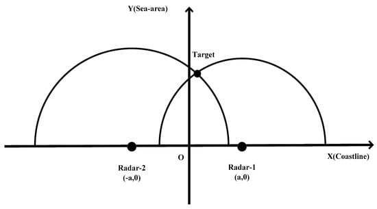
Figure 1.
Schematic diagram of the stereoscopic High frequency surface wave radar (HFSWR) system.
At time point k, the state is described as
where and describe the position of the vessel, and and represent the vessel velocity along the x and y direction, respectively. For the constant velocity (CV), constant acceleration (CA), and constant turn (CT) model [23], the state equation can easily be obtained:
The observation vector is described as
where and are the radial range, and and are the radial velocity. The measurement model is
where the observation noise is zero mean Gaussian white noise. Based on the geometrical relationship between the state and the measurement, the nonlinear measurement function can be determined accordingly:
The process of the target fusion and tracking algorithm based on IMM is shown in Figure 2, and the specific details of the algorithm are presented below.
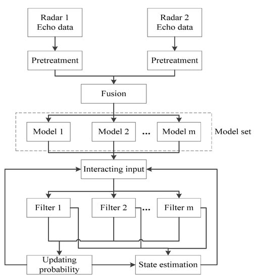
Figure 2.
Flow graph of interacting multiple model extended Kalman filter (IMMEKF).
2.1. Interacting Input
2.2. Model Filtering
2.3. Updating Model Probability
2.4. Estimation Fusion
3. Long-Term Continuous Tracking Method
For conventional tracking methods of HFSWR, the trajectory of vessel targets often breaks in segments due to interferences from other vessels, strong clutters, instant maneuvering, etc. In this section, we present a long-term continuous tracking method on the basis of the ELM network by extracting effective features to associate the track segments of the same vessel.
3.1. ELM Model
As is shown in Figure 3, the extreme learning machine (ELM) is a single hidden layer neural network with low computational complexity and good general performance [24,25]. Compared with the traditional neural network, ELM can randomly initialize the input weight and offset without adjusting during the training process [26], which make it simple and fast with the guarantee of accuracy [27].
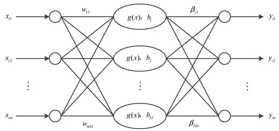
Figure 3.
Extreme learning machine (ELM) network model.
Supposing there are N arbitrary data, the ELM network with M hidden layer nodes can be expressed as follows:
where g(x) is the activation function, is the input weight, is the output weight, and is the bias of the ith node.
The aim of neural network learning is minimizing the output error, which can be expressed as follows:
where is the output of the hidden layer, is the output weight, is the output of mathematical expectation, and is the Moore-Penrose generalized inverse of matrix .
3.2. Feature Extraction
In order to sufficiently reflect the track segment features, we associate the tracks based on features extracted from track segments rather than comparing the distances of track segments point by point. To improve the tracking performance in a complex environment, more features should be extracted for track association. In this paper, we selected the average velocity, average curvature, ratio of the arc length to the chord length, and the wavelet coefficient as the feature vectors to train and test the ELM.
3.2.1. Average Velocity ()
Velocity as an inherent property varying with vessels can be reflected in the track segments, and thus we select the average velocity of the track segment as an important characteristic variable, which is defined as follows:
where is the velocity component of the vessel along the x axis, and is the velocity component of the vessel along the y axis.
3.2.2. Average Curvature ()
Curvature is the rate of change of the angle between the tangent of a point on the curve and the x axis relative to the arc length, which is defined by differentiation to indicate the degree of deviation of the curve from a straight line. The average curvature represents the deviation and regression degree of the course, which reflects the course correction ability varying with vessels under the interference of wind and waves. The average curvature () is defined as follows:
where is the first derivative of the arc length, and is the second derivative of the arc length.
3.2.3. Ratio of the Arc Length to the Chord Length ()
The arc length is the invariant of smooth curved motion, and the chord length has similar invariance. The ratio of the arc length to the chord length can roughly reflect the deviation and regression degree of course varying with vessels under the interference of wind and waves, which is similar to the average curvature. The ratio of the arc length to the chord length is defined as follows:
where is the chord length, and is the arc length.
3.2.4. Wavelet Coefficient
Wavelet transform is a multi-resolution signal analysis method. It assumes that the measurement sequence is a non-stationary sequence with polynomial trend. After a wavelet transformation, can be reconstructed as
where is the high frequency coefficient reflecting the overall situation of the track and is the low frequency coefficient reflecting the change of the target movement. In the frequency domain, the trend of the signal is represented by the low frequency part of the signal, which is represented by the low frequency coefficient in a wavelet analysis. The low frequency coefficient of a two-scale wavelet transformation based on the Haar function is taken as a track feature, which can represent the trend of the track segment.
3.3. Procedure of the Tracking Method Based on an IMMEKF Combined with an ELM
The procedure of the target tracking method based on an IMMEKF combined with an ELM is shown in Figure 4. Track segments are obtained by the IMMEKF when tracking the maneuvering target using the stereoscopic HFSWR data, and simultaneously, the ELM decides whether the newly obtained track segment associates with the former segment via feature classification. In this way, the method can achieve long-term continuous tracking of the vessel target.

Figure 4.
Flow graph of the continuous tracking method based on IMMEKF combined with ELM.
4. Experiment Results
4.1. Simulation Experiment
We assume that the radar monitoring area is approximately 20 km to 38 km in the x axis and approximately 20 km to 32 km in the y axis, where four vessels maneuvering with multiple models are simulated with MATLAB (MathWorks, Natick, MA, USA). For the conventional tracking method [13], the vessel track breaks into segments, as shown in Figure 5a. Combined with a trained ELM network, the proposed method realizes correct track segment association. As is shown in Figure 5b, different types of track segments are colored according to the classification results obtained by the ELM.
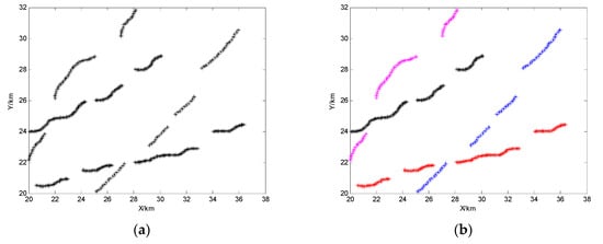
Figure 5.
Results of a simulation experiment: (a) track segments obtained by a conventional tracking method; (b) association results of the proposed method.
In order to verify the rationality and superiority of the proposed method, we carried out simulations on the basis of different combinations of features and different machine learning methods. To evaluate the association performance, the correct association probability (), the error association probability () and the missing association probability () are defined as follows:
where represents the total number of track segments in the experiment, represents the number of correctly associated track segments, represents the number of incorrectly associated track segments, and represents the number of missed track segments.
4.1.1. Simulations Based on Different Combinations of Features
Among the four proposed features, is an inherent property varying with vessels and reflects the overall movement trend of the track segment, while both and reflect the degree of deviation and regression of vessels under the interference of wind and waves, respectively. We carried out simulations on the basis of different combinations of features. As is shown in Table 1, is more effective than in characterizing the features of track segments, and the correct association probability reaches the highest when they work together, which illustrates that and can reinforce one another in reflecting the degree of deviation and regression of vessels. Therefore, the proposed method in this paper selects all four of these features to work together for better association performance.

Table 1.
Statistical results of track segment association based on different features (%).
4.1.2. Simulations Based on Different Machine Learning Methods
We carried out simulations based on different machine learning methods to show the performance of an ELM. As is shown in Table 2, the ELM has the fastest speed and the highest accuracy compared with the back propagation (BP) network and the SVM. Moreover, the ELM is more efficient than the BP and the SVM. Hence, we selected the ELM to combine with the IMMEKF in the proposed method in this paper to achieve long-term continuous tracking of multiple targets.
Table 2.
Statistical results of track segment association based on different machine learning methods. BP: back propagation; SVM: support vector machine.
4.1.3. Comparison between the Conventional TSA Algorithm and the Proposed Method
The above simulations show that the extracted features of the track segment based on an IMMEKF can adequately reflect the vessel’s attributes and motion characteristics; even better, the ELM can effectively learn the features of different track segments and accurately classify them. Furthermore, we carried out simulations comparing the conventional TSA algorithm and the proposed method. As is shown in Table 3, the proposed method has better performance than the conventional TSA algorithm.
Table 3.
Statistical results of track segment association based on simulation (%). TSA: track segment association.
4.2. Field Experiment
To compare the performance of the conventional TSA algorithm and the proposed method, we conducted extensive experiments basing the field data collected by a stereoscopic HFSWR system located on the northern shore of Weihai, China, on 21 July 2019. Data from an AIS (automatic identification system) is defined as the ground truth, which includes the number plates of the vessels of each track segment.
We selected the track as an example in Figure 6, where track segments x and y, marked with “*” and “+”, respectively, are the tracks of vessel A, and segment z, marked with “°”, is the track of vessel B. Although x is close to z, the ELM can determine that the track trend and characteristics between x and y are consistent, which are from the same target. The proposed method associated the track segment correctly in Figure 6c, yet the conventional TSA algorithm associated the track incorrectly in Figure 6b.
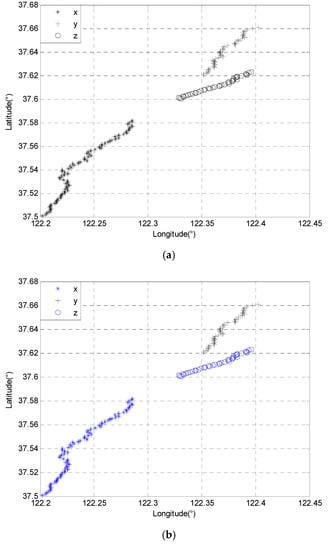
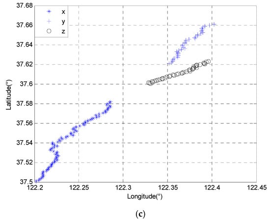
Figure 6.
Comparison of track association results: (a) track segments from field data; (b) association results of the conventional TSA algorithm; (c) association results of the proposed method.
On the basis of 60 track segments obtained from field data, we calculated the average correct association probability, average error association probability, and average missing association probability of the two methods. The statistical results are shown in Table 4. Compared with the conventional TSA algorithm, the average correct association probability of the proposed method was increased by 21.7%, and the average error association probability and average missing association probability of the proposed method were reduced by 5.0% and 16.7%, respectively. Hence, the method proposed in this paper can effectively solve the problem of track segment association, which can effectively overcome the track breaking caused by strong sea clutter interference and interference from other vessels near dense channels, and realize the long-term continuous tracking of a specific vessel target with higher accuracy and stronger adaptability.
Table 4.
Statistical results of track segment association based on radar data (%).
5. Discussion
In Section 4.1.1, simulations were carried out on the basis of different combinations of features, which illustrates that the association performance is the best when the four extracted features of the tracks work together; in Section 4.1.2, we gave a comparison among different machine learning methods, which shows that the ELM had the fastest speed and the highest accuracy compared with the BP network and the SVM. Hence, we selected the ELM and all four of those features working together in the proposed method to realize track segment association. In Section 4.2, the proposed method was verified to have a better performance compared with the conventional TSA algorithm on the basis of radar data.
There is no doubt that the method proposed in this paper can effectively improve the track continuity of the target and realize the long-term continuous tracking of a specific vessel target. Moreover, the new method is easy for engineering implementation due to its generality, simple structure, reduced calculations, high learning speed, and high accuracy. In future research, we will consider further mining features of track segments and improving the network structure of the ELM to achieve better association accuracy.
6. Conclusions
We proposed a long-term continuous tracking method for vessel targets with stereoscopic HFSWR based on an IMMEKF combined with an ELM to solve the problem of trajectory breaking in large-scale marine surveillance. The IMMEKF is applied for the vessel target tracking, meanwhile the ELM network is combined to judge whether the present track is associated with the former track segments. For fully embodying the characteristics of track segments, we selected the average velocity, average curvature, ratio of the arc length to the chord length, and the wavelet coefficient as the feature vectors to train and test the ELM. The tracking algorithm IMMEKF and the track segments associating scheme of the ELM work simultaneously and iteratively. Both the simulation and the field experiment results showed that the proposed method has better tracking performance than the conventional algorithms, with an average correct track segment association rate of over 91.2%. Further, field experiment data from stereoscopic onshore HFSWR located in Weihai showed that the ELM-based track association method had higher accuracy, with lower error and missing association probability due to effective features extracted from the track segments. The method can effectively solve the problem of track fracture caused by rapid maneuvering, strong clutter, target occlusion, long sampling intervals, low detection probabilities, and interference from other vessels near channels, providing a new way for long-term continuous tracking of vessel targets in complex environments. Moreover, the new method is efficient and easy to implement due to its simple structure, which allows the real-time tracking of vessel targets for stereoscopic HFSWR.
Author Contributions
Conceptualization: L.Z.; Methodology: D.M. and L.Z.; Software: D.M. and J.N.; Validation: J.N. and D.M.; Investigation: D.M.; Resources: Y.J.; Data Curation: Y.J.; Writing—Original Draft Preparation: L.Z. and D.M.; Project Administration: Y.J.; Writing—Review and Editing: Q.M.J.W. All authors have read and agreed to the published version of the manuscript.
Funding
This project is sponsored by National Key R&D Program of China (No. 2017YFC1405202), and the National Natural Science Foundation of China (No. 51979256, No. 61671166, No. 41506114).
Conflicts of Interest
The authors declare no conflict of interest. The funders had no role in the design of the study; the collection, analyses, or interpretation of data; the writing of the manuscript; or the decision to publish the results.
References
- Grosdidier, S.; Baussard, A. Ship detection based on morphological component analysis of high-frequency surface wave radar images. IET Radar Sonar Navig. 2012, 6, 813–821. [Google Scholar] [CrossRef]
- Zhang, L.; You, W.; Wu, Q.M.; Qi, S.B.; Ji, Y.G. Deep learning-based automatic clutter/interference detection for HFSWR. Remote Sens. 2018, 10, 1517. [Google Scholar] [CrossRef]
- Pan, S.S.; Bao, Q.L.; Hou, W.B.; Che, Z.P. An improved track segment association algorithm using MM-GNN method. In Proceedings of the 2017 Progress in Electromagnetics Research Symposium Spring—(PIERS), St Petersburg, Russia, 22–25 May 2017; pp. 675–681. [Google Scholar]
- Raghu, J.; Srihari, P.; Tharmarasa, R.; Kirubarajan, T. Comprehensive track segment association for improved track continuity. IEEE Trans. Aerosp. Electron. Syst. 2018, 1, 2463–2480. [Google Scholar] [CrossRef]
- Bar-Shalom, Y. On the track-to-track correlation problem. IEEE Trans. Autom. Control. 1981, 26, 571–572. [Google Scholar] [CrossRef]
- Yeom, S.W.; Kirubarajan, T.; Bar-Shalom, Y. Track segment association, fine-step IMM and initialization with Doppler for improved track performance. IEEE Trans. Aerosp. Electron. Syst. 2004, 40, 293–309. [Google Scholar] [CrossRef]
- Zhang, S.; Bar-Shalom, Y. Track segment association for GMTI tracks of evasive move-stop-move maneuvering targets. IEEE Trans. Aerosp. Electron. Syst. 2011, 47, 1899–1914. [Google Scholar] [CrossRef]
- Aybars, T.; Ali, K.H. A fast track to track association algorithm by sequence processing of target states. In Proceedings of the 2018 21st International Conference on Information Fusion (FUSION), Cambridge, UK, 10–13 July 2018; pp. 1280–1284. [Google Scholar]
- Zhu, H.; Wang, C. Joint track-to-track association and sensor registration at the track level. Digit. Signal. Process. 2015, 41, 48–59. [Google Scholar] [CrossRef]
- Ashraf, M.A.; Murali, T.; Roberto, C. Fuzzy logic data correlation approach in multisensor–multitarget tracking systems. Signal. Process. 1999, 76, 195–209. [Google Scholar]
- Stubberud, S.C.; Kramer, K.A. Data association for multiple sensor types using fuzzy logic. In Proceedings of the IEEE Instrumentation & Measurement Technology Conference, Ottawa, ON, Canada, 17–19 May 2005; pp. 2154–2159. [Google Scholar]
- Shao, H.; Japkowicz, N.; Abielmona, R.S. Vessel track correlation and association using fuzzy logic and Echo State Networks. In Proceedings of the 2014 IEEE Congress on Evolutionary Computation (CEC), Beijing, China, 6–11 July 2014; pp. 2322–2329. [Google Scholar]
- Hong, S.X.; Peng, D.L.; Shi, Y.F. Track-to-track association using fuzzy membership function and clustering for distributed information fusion. In Proceedings of the 37th Chinese Control Conference, Wuhan, China, 25–27 July 2018; pp. 4028–4032. [Google Scholar]
- Siwei, L.; Wujie, Y.; Aijun, Z. Performance of feedback BP networks. J. Syst. Eng. Electron. 1995, 6, 11–18. [Google Scholar]
- Xie, J.; Zhou, J. Classification of urban building type from high spatial resolution remote sensing imagery using extended MRS and soft BP network. IEEE J. Sel. Top. Appl. Earth Obs. Remote Sens. 2017, 1, 3515–3528. [Google Scholar] [CrossRef]
- Liu, X.; Tang, J. Mass classification in mammograms using selected geometry and texture features, and a new SVM-based feature selection method. IEEE Syst. J. 2014, 8, 910–920. [Google Scholar] [CrossRef]
- Pal, M.; Mather, P.M. Support vector machines for classification in remote sensing. Int. J. Remote Sens. 2005, 26, 1007–1011. [Google Scholar] [CrossRef]
- Lu, X.; Zou, H.; Zhou, H.; Xie, L.; Huang, G.B. Robust extreme learning machine with its application to indoor positioning. IEEE Trans. Cybern. 2016, 46, 194–205. [Google Scholar] [CrossRef] [PubMed]
- Huang, G.B.; Wang, D.H.; Lan, Y. Extreme learning machines: A survey. Int. J. Mach. Learn. Cybern. 2011, 2, 107–122. [Google Scholar] [CrossRef]
- Levine, S.; Pastor, P.; Krizhevsky, A.; Quillen, D. Learning hand-eye coordination for robotic grasping with deep learning and large-scale data collection. Int. J. Robot. Res. 2016, 1, 173–184. [Google Scholar] [CrossRef]
- Shin, H.C.; Roth, H.R.; Gao, M.C.; Lu, L.; Xu, Z.; Nogues, I.; Yao, J.H.; Mollura, D.; Summers, R.M. Deep convolutional neural networks for computer-aided detection: CNN architectures, dataset characteristics and transfer learning. IEEE Trans. Med. Imaging 2016, 35, 1285–1298. [Google Scholar] [CrossRef] [PubMed]
- Zhang, L.; Jiang, Y.; Li, Y.S.; Li, G.S.; Ji, Y.G. Adaptive maneuvering target tracking with 2-HFSWR multisensor surveillance system. IEEE Aerosp. Electron. Syst. Mag. 2017, 32, 70–76. [Google Scholar] [CrossRef]
- Bahar, E.; Kurt, G.K. Location estimation in multi-carrier systems using extended Kalman based interacting multiple model and data fusion. In Proceedings of the 2011 IEEE Symposium on Computers and Communications (ISCC), Kerkyra, Greece, 28 June–1 July 2011; pp. 469–471. [Google Scholar]
- Huang, G.B.; Zhu, Q.Y.; Siew, C.K. Extreme learning machine: A new learning scheme of feedforward neural networks. In Proceedings of the 2004 IEEE International Joint Conference on Neural Networks, Budapest, Hungary, 25–29 July 2004; pp. 489–501. [Google Scholar]
- Huang, G.B.; Zhu, Q.Y.; Siew, C.K. Extreme learning machine: Theory and applications. Neurocomputing 2006, 70, 489–501. [Google Scholar] [CrossRef]
- Zong, W.; Huang, G.B. Face recognition based on extreme learning machine. Neurocomputing 2011, 74, 2541–2551. [Google Scholar] [CrossRef]
- Rong, H.J.; Huang, G.B.; Sundararajan, N. Online sequential fuzzy extreme learning machine for function approximation and classification problems. IEEE Trans. Syst. Man Cybern. Part B 2009, 39, 1067–1072. [Google Scholar] [CrossRef] [PubMed]


© 2020 by the authors. Licensee MDPI, Basel, Switzerland. This article is an open access article distributed under the terms and conditions of the Creative Commons Attribution (CC BY) license (http://creativecommons.org/licenses/by/4.0/).