Abstract
Sugar beet is one of the main crops for sugar production in the world. With the increasing demand for sugar, more desirable sugar beet genotypes need to be cultivated through plant breeding programs. Precise plant phenotyping in the field still remains challenge. In this study, structure from motion (SFM) approach was used to reconstruct a three-dimensional (3D) model for sugar beets from 20 genotypes at three growth stages in the field. An automatic data processing pipeline was developed to process point clouds of sugar beet including preprocessing, coordinates correction, filtering and segmentation of point cloud of individual plant. Phenotypic traits were also automatically extracted regarding plant height, maximum canopy area, convex hull volume, total leaf area and individual leaf length. Total leaf area and convex hull volume were adopted to explore the relationship with biomass. The results showed that high correlations between measured and estimated values with R2 > 0.8. Statistical analyses between biomass and extracted traits proved that both convex hull volume and total leaf area can predict biomass well. The proposed pipeline can estimate sugar beet traits precisely in the field and provide a basis for sugar beet breeding.
1. Introduction
Sugar beet ranks as the second largest crop for sugar production in the world and the first in Europe. It is also the source for bioethanol and animal feed [1,2]. According to the prediction of per capita sugar consumption and population growth, the world sugar production is about 175 metric tons at present, and needs to be increased by one million tons every year to meet the demand of 230 million tons in 2050 [3,4]. To improve global sugar production, plant breeding programs need to find the desired sugar beet genotypes to meet the requirements [2,5]. However, plant phenotyping, as a key to plant breeding programs [6,7], is usually performed manually which is time-consuming and expensive [8,9]. Thus, plant phenotyping becomes a bottleneck in many breeding programs.
To speed up and improve plant phenotyping, two-dimensional (2D) solutions have emerged in recent years, such as some semi-automated solutions based on 2D image for phenotyping of leaf and root [10,11,12,13]. However, due to the loss of one dimension information (e.g., thickness, bending, rolling and orientation) when transposing the data from three dimensions (3D) to 2D [14,15,16], these solutions struggled to estimate plant phenotypic traits precisely. Nowadays, several sensor-based 3D technologies have been used in plant phenotyping and can be divided into two categories: active and passive sensors [17]. Active sensors emit its own light source independent of external light, such as hand-hold laser scanning (LS) [18,19], structured light (SL) [20,21], terrestrial laser scanning (TLS) [22,23] and time of flight (TOF) [24,25]. These active technologies have good resolutions and can be applied to different phenotyping scales. However, they are expensive, especially for LS and TLS [17,26].
Structure from motion (SFM), featured as lightweight and cheap [17,26], is a commonly used passive technology in phenotypic traits quantification [27,28], biomass estimation [29,30] and yield prediction [31]. A previous study achieved high precision for leaf area and volumetric shape of taproots of sugar beet in the laboratory [18]. To our knowledge, quantification of 3D architecture of sugar beet growing in the field is still missing. The conditions in the field are much more complicated than that in laboratory, such as serious occlusion between plants, wind and light condition etc. Many technologies (e.g., SL, TOF) have difficulty in obtaining complete point cloud of individual plant caused by occlusions between plants or overlapping between leaves in the field. Structure from motion technique can reduce the effect of occlusion by adding pictures from different viewpoints. The more data collected from different points of view, the more complete the point cloud of individual plant obtained [17].
The overall aim of this study is to dynamically quantify aboveground structure of individual sugar beet plant growing in the field based on SFM method. The specific goals are to: (a) reconstruct 3D point cloud of individual plant based on SFM method; (b) develop an automatic data processing pipeline to process point cloud of individual plant and extract phenotypic trait values, such as plant height, maximum canopy area, convex hull volume, total leaf area and individual leaf length; (c) explore the possibilities of using the extracted phenotypic trait values for sugar beet biomass estimation.
2. Materials and Methods
2.1. Experimental Design and Data Acquisition
The experimental site is located at the Liangcheng experimental station, Inner Mongolia, China (40.502261 N, 112.145304 E) with an altitude of 1459.24 m. There were 20 planting plots in the experimental area of 88 m2 (8 m × 11 m). The area of each plots was 1.2 × 2.3 m. Twenty genotypes of sugar beets were planted. The sowing time was 20 May 2019. The plant spacing was 0.25 m, and row spacing was 0.4 m. The spacing between the plots was 0.5 m. The field management of all plots was the same.
The sugar beet plants were sampled at 69 (T1), 96 (T2) and 124 (T3) days after emergence. In each period, 20 plants were randomly sampled. We used Canon 800D digital camera (Canon, Inc., Tokyo, Japan) to capture multi-view images of individual plant with 6000 × 4000 resolution in situ. Photographing was taken in two circles around the plant and the overlapping area between the two adjacent images was about 70–80%, in order to capture the feature points across-the-board from side view and top view (Figure 1). After taking images, the manual measurements of individual plant were performed, including height and fresh biomass of aboveground. The plant height was measured as the vertical distance between the base of the stem to the highest point of the plant. Fresh biomass was obtained using an electronic balance.
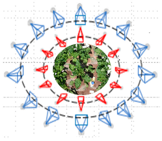
Figure 1.
Camera positions for the multi-view images. Red cameras are from top view and blue cameras are from side view.
2.2. Data Process
The process flow of multi-view images was shown as Figure 2, including following steps on point clouds of individual plant: (1) Reconstruction and preprocessing (Figure 2a,b); (2) Coordinates correction (Figure 2c–e); (3) Filtering and segmentation (Figure 2f,h); (4) Extraction of phenotypic traits of aboveground (Figure 2g,i), involving plant height, maximum canopy area, convex hull volume, total leaf area and individual leaf length.
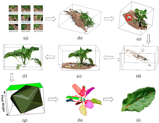
Figure 2.
Data process flow: (a) Multi-view image set of sugar beet in the field; (b) Reconstructed point cloud of sugar beet population; (c) Individual point cloud of sugar beet. The red square is the magic cube; (d) Extracted point cloud of ground plane, represents the normal vector of ground plane and stands for unit vector of z-axis; (e) Point cloud of sugar beet after coordinates correction; (f) Point cloud of sugar beet after filtering; (g) Plant structure extraction of sugar beet, green part means maximum canopy area; (h) Point cloud of sugar beet after segmentation; (i) Leaf structure extraction, the red line represents the extracted leaf length.
2.2.1. Reconstruction and Preprocessing of Point Clouds
The 3DF Zephyr Aerial software was used to reconstruct point cloud of individual sugar beet from multi-view image set based on multi-view stereo and structure from motion (MVS-SFM) algorithm (Figure 2a,b). The SFM algorithm can generate sparse point clouds from multi-view image set. During the process, a scale-invariant feature transform (SIFT) keypoints detector [32], which is featured as invariant to image translation, scaling and rotation, was used to detect keypoints in multi-view images. An approximate nearest neighbor (ANN) algorithm [33] was adopted to match keypoints from multi-view images. Then, projection matrix and 3D point coordinates were correspondingly calculated. The MVS algorithm can turn sparse point clouds into dense point clouds.
For reconstructed point cloud, the coordinate is unitless. A magic cube (Figure 2c) with 5.5 cm side length was adopted to obtain actual size of sugar beet point cloud. In addition, point cloud of individual sugar beet (Figure 2c) was extracted from sugar beet population using CloudCompare (http://www.danielgm.net/cc/; 3D point cloud and mesh processing software) manually.
2.2.2. Coordinates Correction of Point Cloud
In order to correct the coordinates of point cloud as z-axis perpendicular to the ground, we need to find the rotation matrix from the ground normal vector to the z-axis vector at current coordinate system. Then, the rotation matrix is applied to point cloud of individual plant. First of all, the ground plane equation (Equation (1)) of point cloud was calculated using the Random Sample Consensus (RANSAC) algorithm [34], listed as follows:
Then, according to the ground plane equation, we can easily obtain the vector (A, B, C) as the normal vector of the ground plane. The vector (0, 0, 1) was the z-axis vector (Figure 2d).
The angle between and can be calculated by the following formulae:
where m and n are the length of and , respectively. The vector of rotation axis of two vectors ( and ) must be perpendicular to the plane formed by these two vectors. Thus, the vector can be computed by the following formula:
The unit vector of the vector can be calculated by the vector . With the unit vector of rotation axis and rotation angle , the rotation matrix from to can be obtained by Rodrigues’ rotation formula (Equation (5)):
where E is a third order unit matrix, is a rotation angle and the unit vector of rotation axis = (d1, d2, d3).
Finally, the point cloud of individual plant after coordinate correction (Figure 2e) can be obtained by the following formula:
where (x, y, z) is origin coordinate and (x1, y1, z1) is corrected coordinate.
2.2.3. Filtering and Segmentation of Point Cloud
As the influence of light, wind and other factors in the field environment the point cloud will inevitably contain some noise. The extraction of plant structure will be affected. Therefore, the filtering needs to be performed to remove noise points and outliers in order to obtain a smoother plant dense points cloud. There are three classes of points in reconstructed point cloud: plant, soil and shadows (Figure 2e). We selected G minus R (G-R) as color filter and calculated the G-R mean values of point cloud in three periods (T1, T1, T3). We found that the color filter divided point cloud into three categories. The G-R values represent plants, shadows and soil from larger to small value (Figure 3). The value 7 of (G-R) between plants and shadows points was chosen to eliminate soil and shadows points from plant. Outliers were removed based on statistical filter (Figure 2f).
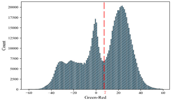
Figure 3.
Histogram of mean G-R difference for point cloud in three periods (T1, T2, T3). The red dotted line is value 7 of (G-R), separating plants from soils and shadows.
The region-growing algorithm [35] was utilized to segment plant into individual leaves (Figure 2h). The algorithm grows from the point with the smallest curvature (seed point) and classifies neighbor points with small normal deviation into the same category. If the normal deviation of a neighbor point exceeds the threshold but the curvature deviation remains within the threshold, the point will be the next seed point. If the curvature deviation and normal deviation of a neighbor point both exceed threshold, the point will be discarded.
For plants with flat leaves, the region-growing algorithm performs well. While for plants with curved leaves, certain parts of curved leaves will be discarded. Therefore, clustering based on Euclidean distance was used to cluster discarded points on the leaves which they originally belonged to.
2.2.4. Structure Extraction of Plant Aboveground
Five phenotypic traits were extracted from the processed point cloud of individual plant, including plant height, maximum canopy area, convex hull volume, total leaves area and individual leaf blade length. The base of the stem to the highest point of the plant is defined as the plant height (Figure 2g). Maximum canopy area is calculated from the product of the maximum length and maximum width of the canopy (the green part in Figure 2g). Total leaf area is the sum of individual leaf area of the whole plant. These traits can be classified into two categories: (a) global traits and (b) organ-level traits. Global traits quantify the overall plant morphology, such as plant height, maximum canopy area, convex hull volume and total leaves area. Organ-level traits focus on the individual organs of plant, such as leaf blade length.
As the coordinates of point cloud of individual plant have been corrected, we can estimate plant height using:
where and are the z-coordinate of the tallest and the shortest points among the point clouds of individual plant, respectively. The quick hull algorithm [36] was adopted to build a convex hull for point cloud of individual plant as shown with the dark green hull in Figure 2g). The calculation of each leaf area is based on the leaf mesh. The following steps were performed: (a) Use the Moving Least Squares (MLS) [37] algorithm for point cloud smoothing and improve normal estimation; (b) Build a mesh for leaf point cloud using the marching cubes algorithm [38]. (c) Calculate the sum of each triangle area using Helen’s formula (Equation (8)) as the leaves’ area:
where S is the area of a triangle, p is the half of perimeter of triangle and a, b and c are the lengths of the three sides of the triangle.
Accurate estimation of leaf blade length largely relies on the endpoints of leaf midrib. In this study, the leaf base point is defined as the point closest to the main stem. However, there is no obvious main stem for sugar beet. Thus, the line parallel to the Z axis and passed through the midpoint of the bounding box is defined as the main stem. After obtaining the base point, the tip point of leaf blade is defined as the point farthest from a line, which is parallel to the Z axis and passing through the base point. Once finding the base and tip points of the leaf, we needed to rotate the leaf base and tip points to the same axis to reduce leaf midrib dimension from 3D to 2D. First of all, the leaf blade was translated so that the base point of leaf blade was at the coordinate origin. The point cloud of leaf blade needs to be rotated radians around the z-axis (anti-clockwise) so that the tip point is on the y-axis. The can be calculated by following formula:
where x and y are the x-axis and y-axis of tip point, respectively. Finally, polynomial regression-fitting algorithm [39] was used to smooth midrib of leaf blade and shown with the red line in Figure 2i.
2.3. Performance Evaluation
Sixty sugar beets with one or two leaves randomly selected from each plant were used for performance evaluation. Linear regression analyses were performed between the manual measurements and the estimation values for plant height and leaf blade length. The following statistics were calculated for performance evaluation: correlation coefficient (r) and root mean square error (RMSE, Equation (10)):
where n is the number of samples; and are the estimation value and manual measurement, respectively.
Univariate linear regression was used to find the relationship between extracted plant traits (total leaf area and convex hull volume) and fresh biomass. The r value was calculated to evaluate the relationships between the fresh biomass and those estimation traits.
3. Results
3.1. Processing of Point Cloud of the Individual Plant
3.1.1. Filtering of Point Cloud of the Individual Plant
Figure 4 showed the histograms of G-R mean value of sugar beet at different growth periods. The color filter G-R performed well for separating sugar beet from soils and shadows at three periods. There were small differences of the separating thresholds among three periods (8.5 at T1 period, 6.5 at T2 period and 7.5 at T3 period). Therefore, we selected a G-R difference of 7 as threshold to filter all point cloud of individual plant at three periods. Figure 5 showed an example of filtering process for one sugar beet. Sugar beet plant, shadows and soils were clearly separated with completely different colors (Figure 5b). After color filtering, the leaf with shadow could remain complete (Figure 5c). Some outliers existed in the point cloud of individual plant after color filtering (Figure 5c) and eliminated completely with statistical filtering (Figure 5d).
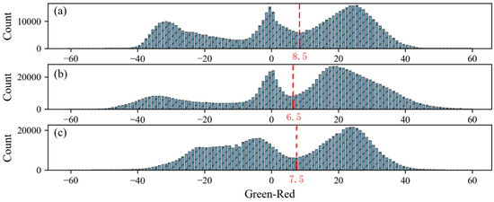
Figure 4.
G-R mean value of all sugar beet point clouds at (a) T1, (b) T2 and (c) T3 period. The red dotted line is the (G-R) value separating plants from soils and shadows.
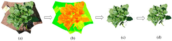
Figure 5.
Performance of filtering: (a) Point cloud of individual plant after coordinate correction; (b) G-R color distribution of point cloud; points with dark green represent soils; points with light green represent shadows; points with orange represents plant; (c) Point cloud of individual plant after color filtering; (d) Point cloud of individual plant after statistical filtering.
3.1.2. Segmentation of Point Cloud
Point clouds of individual plant at three growth stages were presented in Figure 6. Both leaf number and total leaf areas increased rapidly from stages T1 to T2, as T1 is a fast-growing stage for sugar beets. When it came to stage T3, most of the leaves became curved and withered. In the current study, we classified 20 genotypes of sugar beets into two plant types according to their appearances (Figure 6). If leaves were more scattered, they can be easily distinguished, especially in stage T3 (Figure 6a). If leaves gathered together, it was very difficult to separate them from each other, especially in stage T2 (Figure 6b).
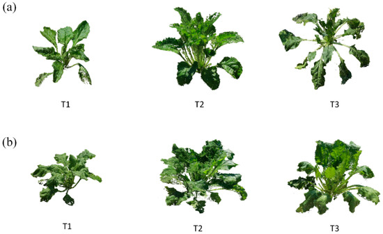
Figure 6.
Point cloud of individual plant at three growth stages (T1, T2 and T3) with plant type of scattered leaves (a) and gathered leaves (b).
Using the regional-growing algorithm, point clouds of individual leaves were initially separated, shown in Figure 7. Within three stages, the segmentation method performed well at T1 and T3, as the leaves were scattered without much overlaps. However, the leaves were not segmented well at T2 stage. As for point cloud at T2 stage, the middle part of the leaves overlapped significantly (leaves in the blue circle in Figure 7b). Thus, it was hard to separate them into individual leaves. The points of the curved leaves were abandoned after initial segmentation, shown in Figure 7a with a red circle. Considering the close distance between points within the same leaf, the clustering algorithm was further utilized to efficiently find those lost points and keep the integrity of segmented leaf (Figure 8).
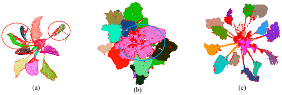
Figure 7.
Point cloud segmentation of sugar beet into individual leaves at (a) T1, (b) T2 and (c) T3 growth stages using regional-growing algorithm. Different colors represent individual leaves at different position on the plant. The red points on each leaf were discarded points at the first segmentation. Leaves in red circle were the curved leaves which lost many points after segmentation. Leaves in blue circle were overlapped with each other at stage T2 and cannot be segmented properly into individual leaves.
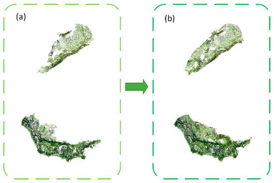
Figure 8.
The effect of the clustering algorithm on point cloud of individual leaves, before clustering (a) versus after clustering (b). The discarded point cloud after segmentation were regathered after clustering to keep the integrity of the segmented leaf.
3.2. Accuracy Assessment
In order to estimate the accuracy of our method, the relationship between estimated plant height and measured height was compared and shown in Figure 9a. Good correlations were found between estimated and measured plant height (R2 = 0.88, RMSE = 5.2 cm). However, most estimated heights were higher than measured values. The estimation accuracy of leaf blade length was also performed and shown in Figure 9b. The high R2 (0.83) and low RMSE (1.77 cm) were found. The fitted line was close to the 1:1 line.
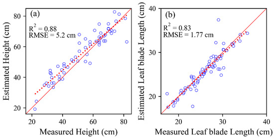
Figure 9.
Comparison of the estimated sugar beet height (a) and the estimated individual leaf length (b) with the measured value.
Several points were far away from 1:1 line in Figure 9a,b, meaning that certain mismatches existed between estimated and measured values. To figure out these mismatches, two cases are shown in figure 10. In the first case, estimated height was much higher than measured height (Figure 10a,b). In the second case, estimated height is different from measured height (Figure 10c,d).

Figure 10.
Two mismatched cases between measured and estimated plant height. (a) Plant A after coordinate correction; (b) Plant A after filtering; (c) Plant B after coordinate correction; (d) Plant B after filtering. Horizontal red lines were ground plane obtained by RANSAC algorithm. Red and blue arrowed lines were measured and estimated height.
Figure 11 showed the extraction results of leaf blade length for two kinds of leaves. Common leaves with upward facing posture (Figure 11a–d) can be fitted well on leaf blade midrib (Figure 11d) with our method. Therefore, the leaf blade length can be calculated well. The twisted leaves (Figure 11e–h) were generally located at the lower part of the plant, not exposing to the sun. They always twisted their petiole and changed their facing directions. Our method can obtain smooth curves for both kinds of leaves (Figure 11c,g). However, our method was not performed well for twisted leaves (Figure 11h). The proportion of twisted leaves to total leaves was very small (three out of 70 leaves in our accuracy assessment). Therefore, our current method did not consider this situation.
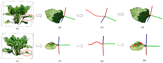
Figure 11.
Leaf blade length extraction for common leaf (a–d) and twisted leaf (e–h). (a,e) Targeted leaf on the plant; (b,f) The display of leaf blade without petiole; (c,g) Extracted curves of midrib; (d,h) The display of extracted curves on leaves.
3.3. Dynamic Estimation of Plant Phenotypic Traits and Biomass
The dynamic changes of plant height, maximum canopy area and convex hull volume were monitored from reconstructed point cloud (Figure 12). The mean value of extracted plant height increased from stages T1 to T2, and peaked at stage T2. Then, plant height decreased slightly from stages T2 to T3. Mean value of maximum canopy area and convex hull volume increased gradually from T1 to T3. Phenotypic traits here varied greatly at stage T3 compared with those at stages T1 and T2. Five points deviated more compared with others regarding plant height, canopy area and convex hull. These were only a very small part compared with the number of experimental plants.
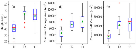
Figure 12.
Distribution of extracted (a) plant height, (b) maximum canopy area and (c) convex hull volume values for sugar beet plants at T1, T2 and T3 stages. The box boundaries represent the 25th and 75th percentiles. Green triangles represent means and red lines represent medians. Red crosses are outliers and the whiskers represent the extreme values of the point cloud.
The fresh weight prediction based on the extracted traits was investigated and shown in Figure 13. At stage T1 and T2, both leaf area and convex hull volume had close relationship with fresh weight with R2 more than 0.80 (Figure 13a,c). The values of leaf area, convex hull volume and fresh weight at T2 were obviously higher than that at stage T1 as the growth of the plants. When incorporating calculated leaf area and convex hull at stage T3, the fitting results with biomass declined (Figure 13b,d). The values of R2 fell to 0.82 and 0.78 for the relationship of fresh biomass with leaf area or with convex hull volume.
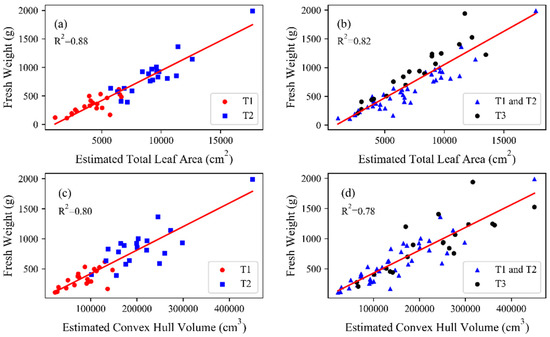
Figure 13.
Correlation of estimated traits and fresh weight: (a) Estimated total leaf area and fresh weight at stages T1 and T2; (b) Estimated total leaf area and fresh weight at stages T1, T2 and T3; (c) Estimated convex hull volume and fresh weight at stages T1 and T2; (d) Estimated convex hull volume and fresh weight at stages T1, T2 and T3.
4. Discussion
4.1. Processing of Point Cloud of Individual Plant
The segmentation plays a very important role in extraction of plant phenotyping but still remains a big challenge [40]. In this study, regional growing algorithm was used to segment plant into individual leaves initially. The algorithm, based on the surface smoothness constraint, was often adopted to segment plants with few flat leaves, such as cucumber, eggplant [41] and maize [42]. However, due to the complex environments in the field, some leaves of sugar beet were curved, which brought a big challenge to the algorithm (Figure 8a). Clustering based on Euclidean distance solved this problem well, and made the segmented leaf to retain complete point cloud (Figure 8b). In addition, the segmentation of plant into individual leaves becomes difficult for the middle and later growth stages because of the overlapping between leaves [39]. In our study, less overlapping leaves were found at stages T1 and T3 compared with stage T2. At stage T2, the overlapping between leaves was so serious that even the manual separation cannot perform well (Figure 7b). As far as we know, fully automatic segmentation has only been realized on broad-leaf plants with few leaves [14] and narrow-leaf crops with few leaves and without tillers [43].
The correction of point cloud of individual plant is essential for estimating plant phenotypic trait, such as plant height and canopy ground cover, etc. The success of correction largely relies on the detection of the ground. The RANSAC algorithm can detect ground and soil plane of pot well [30] in an indoor pot experiment. In our study, the RANSAC algorithm was utilized to detect ground plane (Figure 2d). As the RANSAC algorithm always found the largest plane with the most point cloud as the ground, another smooth plane was detected as base ground due to the uneven ground for field environment as shown in Figure 10c. With the wrong detection of the ground, plant phenotypic traits cannot be estimated well. To avoid this deficiency, the ground point cloud should be preserved as much as possible when the plant population is divided into individual plants (Figure 2b,c).
4.2. Extraction of Plant Phenotypic Traits
Plant height, as a basic phenotypic trait, can be used not only as an intuitive indicator of plant growth state, but also for the estimation of plant biomass and yield [44,45]. In this study, the ground truth of plant height was measured as the vertical distance between the bases of the stem to the highest point of the plant. Estimated plant height was calculated from bounding box of point cloud of individual plant after coordinates correction and filtering (Figure 2g). The estimated plant height was highly correlated with the measured height (R2 = 0.88), but was a little bit higher than the measured value (Figure 9a). It was found that the field ground was uneven, many sugar beet leaves fell on the ground which was lower than base of the stem (Figure 10a). Therefore, the height of the bounding box was often higher than the measured plant height (Figure 10b). Another obvious differences between the measured and calculated plant height were the inaccurate coordinate correction of the plant (Figure 10c,d).
Leaf blade length has been estimated in the literature based on meshes of leave blades [14,26,41]. It was very convenient and accurate to estimate the leaf blade length based on the point cloud of leaf blade. The most important step was to find the base and tip of the leaf blade accurately to calculate leaf blade length. Principal component analysis (PCA) was often adopted to find endpoints of individual leaves [43], but its accuracy was greatly affected by the shape of the leaves. Due to the complex shape of sugar beet grown in the field, we considered the relative position of leaves in the plant as a criterion to find the endpoints of leaves. Researchers have used the shortest path algorithm to find the midrib of leaf blade based on the endpoints on the leaf blade [43], while we rotated the Z-axis so that the endpoints of leaf were on the same axis to find the midrib of leaf blade. Our method can perform well for most of the leaves (Figure 11d). But certain deviation occurred between extracted curve and midrib of leaf blade for twisted leaves, (Figure 11h). Though the twisted leaves occupied less and was always located at the lower part of the plant, a more comprehensive method was still needed to estimate the length of all types of leaves.
4.3. Estimation of Biomass Using Plant Phenotypic Traits
Biomass estimation is important for biological research and agricultural management [46]. Many studies have shown that the total leaf area was highly consistent with biomass [47,48,49]. The correlation between total leaf area and fresh biomass was figured separately in this study with stages T1 to T3 (Figure 12b) and stages T1 to T2 (Figure 12a), and a better performance was found for the latter (R2 = 0.88) compared with the former (R2 = 0.82). Sugar beet grows very fast from stage T1 to T2 and is gradually aged from stage T2 to T3. There were other phenotypic traits involving plant area, such as leaf project area and surface area, that have been used to estimate biomass [29]. The correlations between these phenotypic traits and biomass may be lower than between total leaf area and biomass, but it is easier to measure. In addition, researchers have found that stem volume has more advantages than total leaf area in estimating biomass at the later stage of plant growth [30].
The convex hull and the concave hull are used to describe the volume [36,50]. As researches have shown that the concave hull has poor performance for biomass estimation [29], we only studied the correlation between the convex hull and biomass. Similar to the total leaf area, the estimation of stages T1–T2 is better than that of T1–T3, but the difference is not significant. The biomass estimation with convex hull is obviously inferior to that of total leaf area (Figure 12). Lati [51] used the convex hull to estimate biomass of Black Nightshade. The R2 is much higher than ours (0.88 versus 0.80). Our sugar beets were scattered in stages T1 and T3, but concentrated in stage T2. Only total leaf area and convex hull were used to explore the relationship with fresh weight in the study. More phenotypic traits will be used to predict the fresh and dry weight in the future.
Phenotyping studies of individual plants are usually carried out indoors, but rarely in the field because of the complex environment in the field. The SFM method can get the accurate point cloud of individual plant in the field, which is convenient to extract the organ-level traits accurately. Terrestrial light detection and ranging (lidar) can perform well for the phenotyping of individual plant in the field [52], but very expensive, with more than 100 times the price than common camera. Unmanned Aerial Vehicle (UAV) phenotyping has developed rapidly in recent years. UAV mounted with an rgb camera, lidar or multispectral camera, were always used to obtain point cloud or spectral information more quickly. However, UAV based phenotyping focuses on canopy scale with average height of plants, leaf area index and lodging area. For example, Hu [53] used UAV with an rgb camera to obtain DSM (Digital Surface Model) of sorghum in the field, and estimated the average height of sorghum. Su [54] used UAV with an rgb camera and multispectral camera to estimate average height, canopy leaf area index and lodging area of corn plants. Lei [55] used UAV with lidar to inverse leaf area index of maize and studied the effect of leaf occlusion on inversing leaf area index of maize. As far as we know, UAV with sensors cannot estimate individual organs phenotypic traits very well.
Our research also has limitations. Due to the influence of wind, the shake of plants will bring errors to the reconstruction of 3D model. Zhu [56] used a black and white chessboard pattern of cloth and iron frame as windshield equipment to improve the quality of 3D reconstruction. The influence of wind is very common in the field research. Minimizing the time interval of each data acquisition may be a feasible solution. In addition, the SFM method is convenient for its data collection but time-consuming for its post-process. With the development of GPU computing, the post-processing time has been greatly reduced, but still cannot meet the needs of real-time reconstruction. As the simultaneous localization and mapping (SLAM) is developing rapidly, a more efficient reconstruction algorithm is to be expected in the future. In the next study, more genotypes and phenotypic traits of sugar beet will be extracted for linking genetic with phenotypic traits and provide a basis for sugar beet breeding.
5. Conclusions
In this study, the 3D models of sugar beets for 20 genotypes were reconstructed by SFM method at three growth stages in the field. We developed an automatic pipeline for data processing, including processing of point cloud of individual plant and extraction of plant traits. Segmenting individual plant from plant population manually was the first step of processing of point cloud of individual plant. Then, the soil plane was detected using the RANSAC algorithm, as a criterion to correct the coordinates of point cloud of individual plant. We selected G minus R (G−R) as a color filter to separate plant from soil and shadows and used statistical filter to remove outliers. Finally, regional-growing algorithm was utilized to segment plant into individual leaves and Euclidean distance clustering was used to improve quality of segmented leaves. Extraction of plant traits is other important part of our pipeline. Global traits, such as plant height, maximum canopy area and convex hull volume, were extracted based on the overall structure of plant. Organ-level traits, such as leaf blade length and total leave areas, were extracted based on individual leaves. Plant traits were also used to explore their relationship with sugar beet biomass. Automated measurements from the pipeline showed agreement with the corresponding manual measurements, validating the accuracy and utility of our pipeline. Both the total leaf area and convex hull volume showed potential for biomass prediction (R2 = 0.78–0.88). The pipeline proposed in this study can perform well for estimating plant phenotyping in the field and provide basis for breeding programs.
Author Contributions
Conceptualization, Y.M., Y.S. and R.W.; methodology, S.X.; software, S.X. and H.C.; validation, S.X. and H.C.; formal analysis, S.X.; investigation, H.C., Q.W. and K.S.; resources, Y.M., K.S. and R.W.; data curation, M.S.; writing—original draft preparation, S.X.; writing—review and editing, Y.M.; visualization, S.X.; supervision, Y.M.; project administration, Y.M., Y.S. and R.W.; funding acquisition, Y.M., Y.S. and R.W. All authors have read and agreed to the published version of the manuscript.
Funding
This research was funded by the Science and Technology projects from Inner Mongolia and Yunnan (2017YN07).
Conflicts of Interest
The authors declare no conflict of interest.
References
- Jakiene, E. Effect of the bioorganic fertilizers on sugar beet productivity increase Cukriniu runkeliu produktyvumo optimizavimo tyrimai naudojant bioorganines trasas. Zemes ukio Mokslai 2014, 21, 120–132. [Google Scholar]
- Pegot-Espagnet, P.; Guillaume, O.; Desprez, B.; Devaux, B.; Devaux, P.; Karine, H.; Henry, N.; Willems, G.; Goudemand, E.; Mangin, B. Discovery of interesting new polymorphisms in a sugar beet (elite × exotic) progeny by comparison with an elite panel. Theor. Appl. Genet. 2019, 132, 3063–3078. [Google Scholar] [CrossRef] [PubMed]
- Glover, J.; Cox, C.; Reganold, J. Future farming: A return to roots? Sci. Am. 2007, 297, 82–89. [Google Scholar] [CrossRef] [PubMed]
- Stevanato, P.; Chiodi, C.; Broccanello, C.; Concheri, G.; Biancardi, E.; Pavli, O.; Skaracis, G. Sustainability of the sugar beet crop. Sugar Tech 2019, 21, 703–716. [Google Scholar] [CrossRef]
- Monteiro, F.; Frese, L.; Castro, S.; Duarte, M.; Paulo, O.; Loureiro, J.; Romeiras, M. Genetic and genomic tools to assist sugar beet improvement: The value of the crop wild relatives. Front. Plant Sci. 2018, 1, 74. [Google Scholar] [CrossRef] [PubMed]
- Araus, J.L.; Cairns, J.E. Field high-throughput phenotyping: The new crop breeding frontier. Trends Plant Sci. 2014, 19, 52–61. [Google Scholar] [CrossRef]
- Chaivivatrakul, S.; Tang, L.; Dailey, M.N.; Nakarmi, A.D. Automatic morphological trait characterization for corn plants via 3D holographic reconstruction. Comput. Electron. Agric. 2014, 109, 109–123. [Google Scholar] [CrossRef]
- Richards, R.; Lukacs, Z. Seedling vigour in wheat—Sources of variation for genetic and agronomic improvement. Crop Pasture Sci. 2002, 53, 41–50. [Google Scholar] [CrossRef]
- White, J.W.; Andrade-Sanchez, P.; Gore, M.A.; Bronson, K.F.; Coffelt, T.A.; Conley, M.M.; Feldmann, K.A.; French, A.N.; Heun, J.T.; Hunsaker, D.J. Field-based phenomics for plant genetics research. Field Crops Res. 2012, 133, 101–112. [Google Scholar] [CrossRef]
- Granier, C.; Aguirrezabal, L.; Chenu, K.; Cookson, S.J.; Dauzat, M.; Hamard, P.; Thioux, J.-J.; Rolland, G.; Bouchier-Combaud, S. PHENOPSIS, an automated platform for reproducible phenotyping of plant responses to soil water deficit in Arabidopsis thaliana permitted the identification of an accession with low sensitivity to soil water deficit. New Phytol. 2010, 169, 623–635. [Google Scholar] [CrossRef]
- Bylesjö, M.; Segura, V.; Soolanayakanahally, R.Y.; Rae, A.M.; Trygg, J.; Gustafsson, P.; Jansson, S.; Street, N.R. LAMINA: A tool for rapid quantification of leaf size and shape parameters. BMC Plant Biol. 2008, 8, 82. [Google Scholar] [CrossRef] [PubMed]
- Walter, A.; Scharr, H.; Gilmer, F.; Zierer, R.; Nagel, K.; Ernst, M.; Wiese-Klinkenberg, A.; Virnich, O.; Christ, M.; Uhlig, B.; et al. Dynamics of seedling growth acclimation towards altered light conditions can be quantified via GROWSCREEN: A setup and procedure designed for rapid optical phenotyping of different plant species. New Phytol. 2007, 174, 447–455. [Google Scholar] [CrossRef] [PubMed]
- Jansen, M.; Gilmer, F.; Biskup, B.; Nagel, K.A.; Rascher, U.; Fischbach, A.; Briem, S.; Dreissen, G.; Tittmann, S.; Braun, S. Simultaneous phenotyping of leaf growth and chlorophyll fluorescence via GROWSCREEN FLUORO allows detection of stress tolerance in Arabidopsis thaliana and other rosette plants. Funct. Plant Biol. 2009, 36, 902–914. [Google Scholar] [CrossRef]
- Paproki, A. A novel mesh processing based technique for 3D plant analysis. BMC Plant Biol. 2012, 12, 63. [Google Scholar] [CrossRef]
- Kaminuma, E.; Heida, N.; Tsumoto, Y.; Yamamoto, N.; Toyoda, T. Automatic quantification of morphological traits via three-dimensional measurement of Arabidopsis. Plant J. 2004, 38, 358–365. [Google Scholar] [CrossRef]
- Gibbs, J.A.; Pound, M.; French, A.P.; Wells, D.M.; Murchie, E. plant phenotyping: An active vision cell for three-dimensional plant shoot reconstruction. Plant Physiol. 2018, 178, 524–534. [Google Scholar] [CrossRef]
- Paulus, S. Measuring crops in 3D: Using geometry for plant phenotyping. Plant Methods 2019, 15, 103. [Google Scholar] [CrossRef]
- Paulus, S.; Behmann, J.; Mahlein, A.-K.; Plümer, L.; Kuhlmann, H. Low-cost 3D systems: Suitable tools for plant phenotyping. Sensors 2014, 14, 3001–3018. [Google Scholar] [CrossRef]
- Dupuis, J.; Kuhlmann, H. High-precision surface inspection: Uncertainty evaluation within an accuracy range of 15 μm with triangulation-based laser line scanners. J. Appl. Geod. 2014, 8, 109–118. [Google Scholar] [CrossRef]
- Thuy, N.; David, S.; Nelson, M.; Julin, M.; Neelima, S. Structured light-based 3D reconstruction system for plants. Sensors 2015, 15, 18587–18612. [Google Scholar]
- Geng, J. Structured-light 3D surface imaging: A tutorial. Adv. Opt. Photonics 2011, 3, 128–160. [Google Scholar] [CrossRef]
- Sun, S.; Li, C.; Paterson, A.; Jiang, Y.; Xu, R.; Robertson, J.; Snider, J. In-field high throughput phenotyping and cotton plant growth analysis using LiDAR. Front. Plant Sci. 2018, 9, 16. [Google Scholar] [CrossRef] [PubMed]
- Disney, M. Terrestrial LiDAR: A three-dimensional revolution in how we look at trees. New Phytol. 2019, 222, 1736–1741. [Google Scholar] [CrossRef] [PubMed]
- Zennaro, S.; Munaro, M.; Milani, S.; Zanuttigh, P.; Bernardi, A.; Ghidoni, S.; Menegatti, E. Performance evaluation of the 1st and 2nd generation Kinect for multimedia applications. In Proceedings of the 2015 IEEE International Conference on Multimedia and Expo (ICME), Turin, Italy, 29 June–3 July 2015. [Google Scholar]
- May, S.; Werner, B.; Surmann, H.; Pervolz, K. 3D time-of-flight cameras for mobile robotics. In Proceedings of the 2006 IEEE/RSJ International Conference on Intelligent Robots and Systems, Beijing, China, 9–15 October 2006; pp. 790–795. [Google Scholar] [CrossRef]
- Wang, Y.; Wen, W.; Sheng, W.; Wang, C.; Yu, Z.; Guo, X.; Zhao, C. Maize plant phenotyping: Comparing 3D laser scanning, multi-view stereo reconstruction, and 3D digitizing estimates. Remote Sens. 2018, 11, 63. [Google Scholar] [CrossRef]
- Rose, J.C.; Paulus, S.; Kuhlmann, H. Accuracy analysis of a multi-view stereo approach for phenotyping of tomato plants at the organ level. Sensors 2015, 15, 9651–9665. [Google Scholar] [CrossRef]
- Paulus, S.; Schumann, H.; Kuhlmann, H.; Léon, J. High-precision laser scanning system for capturing 3D plant architecture and analysing growth of cereal plants. Biosyst. Eng. 2014, 121, 1–11. [Google Scholar] [CrossRef]
- Mortensen, A.K.; Bender, A.; Whelan, B.; Barbour, M.M.; Sukkarieh, S.; Karstoft, H.; Gislum, R. Segmentation of lettuce in coloured 3D point clouds for fresh weight estimation. Comput. Electron. Agric. 2018, 154, 373–381. [Google Scholar] [CrossRef]
- Xiang, L.; Bao, Y.; Tang, L.; Ortiz, D.; Fernandez, M. Automated morphological traits extraction for sorghum plants via 3D point cloud data analysis. Comput. Electron. Agric. 2019, 162, 951–961. [Google Scholar] [CrossRef]
- Klodt, M.; Herzog, K.; Töpfer, R.; Cremers, D. Field phenotyping of grapevine growth using dense stereo reconstruction. BMC Bioinform. 2015, 16, 1–11. [Google Scholar] [CrossRef]
- Lowe, D.G. Object recognition from local scale-invariant features. In Proceedings of the Seventh IEEE International Conference on Computer Vision, Kerkyra, Corfu, Greece, 20–27 September 1999. [Google Scholar]
- Arya, S.; Mount, D.M.; Netanyahu, N.S.; Silverman, R.; Wu, A.Y. An optimal algorithm for approximate nearest neighbor searching fixed dimensions. J. ACM 1998, 45, 891–923. [Google Scholar] [CrossRef]
- Fischler, M.A.; Bolles, R.C. Random sample consensus—A paradigm for model-fitting with applications to image-analysis and automated cartography. Commun. ACM 1981, 24, 381–395. [Google Scholar] [CrossRef]
- Rabbani, T.; Heuvel, F.A.V.D.; Vosselman, G. Segmentation of point clouds using smoothness constraint. In Proceedings of the ISPRS Commission V Symposium: Image Engineering and Vision Metrology, Dresden, Germany, 25–27 September 2006. [Google Scholar]
- Barber, C.B.; Dobkin, D.P.; Huhdanpaa, H. The quickhull algorithm for convex hulls. ACM Trans. Math. Softw. 1996, 22, 469–483. [Google Scholar] [CrossRef]
- Alexa, M.; Behr, J.; Cohen-Or, D.; Fleishman, S.; Levin, D.; Silva, C.T. Computing and rendering point set surfaces. IEEE Trans. Vis. Comput. Graph. 2003, 9, 3–15. [Google Scholar] [CrossRef]
- Derose, T.; Duchamp, T.; Mcdonald, J.; Stuetzle, W. Surface reconstruction from unorganized points. ACM Siggraph Comput. Graph. 1992, 26, 71–78. [Google Scholar]
- Duan, T.; Chapman, S.C.; Holland, E.; Rebetzke, G.; Guo, Y.; Zheng, B. Dynamic quantification of canopy structure to characterize early plant vigour in wheat genotypes. J. Exp. Bot. 2016, 67, 4523–4534. [Google Scholar] [CrossRef]
- Paulus, S.; Dupuis, J.; Mahlein, A.K.; Kuhlmann, H. Surface feature based classification of plant organs from 3D laserscanned point clouds for plant phenotyping. BMC Bioinform. 2013, 14, 238. [Google Scholar] [CrossRef]
- Hui, F.; Zhu, J.; Hu, P.; Meng, L.; Zhu, B.; Guo, Y.; Li, B.; Ma, Y. Image-based dynamic quantification and high-accuracy 3D evaluation of canopy structure of plant populations. Ann. Bot. 2018, 121, 1079–1088. [Google Scholar] [CrossRef]
- Zhu, B.; Liu, F.; Che, Y.; Hui, F.; Ma, Y. Three-dimensional quantification of intercropping crops in field by ground and aerial photography. In Proceedings of the 2018 6th International Symposium on Plant Growth Modeling, Simulation, Visualization and Applications (PMA), Hefei, China, 4–8 November 2018; pp. 1–5. [Google Scholar] [CrossRef]
- Elnashef, B.; Filin, S.; Nisim Lati, R. Tensor-based classification and segmentation of three-dimensional point clouds for organ-level plant phenotyping and growth analysis. Comput. Electron. Agric. 2019, 156, 51–61. [Google Scholar] [CrossRef]
- Demir, N.; Sonmez, N.K.; Akar, T.; Unal, S. Automated measurement of plant height of wheat genotypes using a DSM derived from UAV imagery. Proceedings 2018, 2, 5163. [Google Scholar] [CrossRef]
- Guan, H.; Liu, M.; Ma, X.; Yu, S. Three-dimensional reconstruction of soybean canopies using multisource imaging for phenotyping analysis. Remote Sens. 2018, 10, 1206. [Google Scholar] [CrossRef]
- Lati, R.N.; Manevich, A.; Filin, S. Three-dimensional image-based modelling of linear features for plant biomass estimation. Int. J. Remote Sens. 2013, 34, 6135–6151. [Google Scholar] [CrossRef]
- Yang, W.; Guo, Z.; Huang, C.; Duan, L.; Chen, G.; Jiang, N.; Fang, W.; Feng, H.; Xie, W.; Lian, X. Combining high-throughput phenotyping and genome-wide association studies to reveal natural genetic variation in rice. Nat. Commun. 2014, 5, 5087. [Google Scholar] [CrossRef] [PubMed]
- Neilson, E.H.; Edwards, A.M.; Blomstedt, C.K.; Berger, B.; Moller, B.L.; Gleadow, R.M. Utilization of a high-throughput shoot imaging system to examine the dynamic phenotypic responses of a C4 cereal crop plant to nitrogen and water deficiency over time. J. Exp. Bot. 2015, 66, 1817–1832. [Google Scholar] [CrossRef] [PubMed]
- Zhang, X.; Huang, C.; Wu, D.; Qiao, F.; Li, W.; Duan, L.; Wang, K.; Xiao, Y.; Chen, G.; Liu, Q. High-throughput phenotyping and QTL mapping reveals the genetic architecture of maize plant growth. Plant Physiol. 2017, 173, 1554–1564. [Google Scholar] [CrossRef] [PubMed]
- Rusu, R.B.; Cousins, S. 3D is here: Point cloud library (PCL). In Proceedings of the 2011 IEEE International Conference on Robotics and Automation, Shanghai, China, 9–13 May 2011. [Google Scholar]
- Lati, R.N.; Filin, S.; Eizenberg, H. Estimation of plants’ growth parameters via image-based reconstruction of their three-dimensional shape. Agron. J. 2013, 105, 191–198. [Google Scholar] [CrossRef]
- Su, Y.; Wu, F.; Ao, Z.; Jin, S.; Qin, F.; Liu, B.; Pang, S.; Liu, L.; Guo, Q. Evaluating maize phenotype dynamics under drought stress using terrestrial lidar. Plant Methods 2019, 15, 11. [Google Scholar] [CrossRef]
- Hu, P.; Chapman, S.C.; Wang, X.; Potgieter, A.; Duan, T.; Jordan, D.; Guo, Y.; Zheng, B. Estimation of plant height using a high throughput phenotyping platform based on unmanned aerial vehicle and self-calibration: Example for sorghum breeding. Eur. J. Agron. 2018, 95, 24–32. [Google Scholar] [CrossRef]
- Su, W.; Zhang, M.; Bian, D.; Liu, Z.; Huang, J.; Wang, W.; Wu, J.; Hao, G. Phenotyping of corn plants using unmanned aerial vehicle (UAV) images. Remote Sens. 2019, 11, 2021. [Google Scholar] [CrossRef]
- Lei, L.; Qiu, C.; Li, Z.; Han, D.; Han, L.; Zhu, Y.; Wu, J.; Xu, B.; Feng, H.; Yang, H.; et al. Effect of leaf occlusion on leaf area index inversion of maize using UAV-LiDAR data. Remote Sens. 2019, 11, 1067. [Google Scholar] [CrossRef]
- Zhu, B.; Liu, F.; Zhu, J.; Guo, Y.; Ma, Y. Three-dimensional quantifications of plant growth dynamics in field-grown plants based on machine vision method. Trans. Chin. Soc. Agric. Mach. 2018, 49, 256–262. [Google Scholar]
© 2020 by the authors. Licensee MDPI, Basel, Switzerland. This article is an open access article distributed under the terms and conditions of the Creative Commons Attribution (CC BY) license (http://creativecommons.org/licenses/by/4.0/).