Article

Color Calibration of Proximal Sensing RGB Images of Oilseed Rape Canopy via Deep Learning Combined with K-Means Algorithm

1
College of Biosystems Engineering and Food Science, Zhejiang University, Hangzhou 310058, China
2
Key Laboratory of Spectroscopy Sensing, Ministry of Agriculture and Rural Affairs, Hangzhou 310058, China
3
State Key laboratory of Modern Optical Instrumentation, Zhejiang University, Hangzhou 310027, China
4
Agricultural Research Corporation, P.O. Box 126, Wad Medani 11111, Sudan
5
International Centre of Insect Physiology and Ecology (icipe), P.O. Box 30772, Nairobi 00100, Kenya
6
Department of Agronomy, Faculty of Agriculture, University of Khartoum, Khartoum North 13314, Sudan
*
Author to whom correspondence should be addressed.
Remote Sens. 2019, 11(24), 3001; https://doi.org/10.3390/rs11243001
Submission received: 16 October 2019 / Revised: 6 December 2019 / Accepted: 6 December 2019 / Published: 13 December 2019
(This article belongs to the Special Issue Advanced Imaging for Plant Phenotyping)

Abstract

:
Plant color is a key feature for estimating parameters of the plant grown under different conditions using remote sensing images. In this case, the variation in plant color should be only due to the influence of the growing conditions and not due to external confounding factors like a light source. Hence, the impact of the light source in plant color should be alleviated using color calibration algorithms. This study aims to develop an efficient, robust, and cutting-edge approach for automatic color calibration of three-band (red green blue: RGB) images. Specifically, we combined the k-means model and deep learning for accurate color calibration matrix (CCM) estimation. A dataset of 3150 RGB images for oilseed rape was collected by a proximal sensing technique under varying illumination conditions and used to train, validate, and test our proposed framework. Firstly, we manually derived CCMs by mapping RGB color values of each patch of a color chart obtained in an image to standard RGB (sRGB) color values of that chart. Secondly, we grouped the images into clusters according to the CCM assigned to each image using the unsupervised k-means algorithm. Thirdly, the images with the new cluster labels were used to train and validate the deep learning convolutional neural network (CNN) algorithm for an automatic CCM estimation. Finally, the estimated CCM was applied to the input image to obtain an image with a calibrated color. The performance of our model for estimating CCM was evaluated using the Euclidean distance between the standard and the estimated color values of the test dataset. The experimental results showed that our deep learning framework can efficiently extract useful low-level features for discriminating images with inconsistent colors and achieved overall training and validation accuracies of 98.00% and 98.53%, respectively. Further, the final CCM provided an average Euclidean distance of 16.23 ΔΕ and outperformed the previously reported methods. This proposed technique can be used in real-time plant phenotyping at multiscale levels.

Graphical Abstract

1. Introduction

The digital camera has emerged as an essential tool for high-throughput plant phenotyping, and it is widely used to reveal genotypic traits associated with the structure and color of plants. The reliability and repeatability of these traits are highly related to the color constancy of the images [1]. However, images acquired using different digital cameras (or the same camera with changing its settings) produce an inconsistent color, due to the different specifications (e.g., spatial resolution, spectral responses, and signal-to-noise ratio). Moreover, images captured using the same camera at different points in time and dates could vary in color, despite no changes in the object (e.g., plant) characteristics. In such cases, the variability in the image color is a result of sunlight intensity, sun inclination angle, temperature, and other prevailing weather conditions. Such variations in image color have a serious influence on the evaluation of plant physical, chemical, and biological characteristics when color is considered as a relevant and significant trait in studying plant phenotyping [2,3].
Color is an important feature that needs to be automatically characterized by the computer vision-based plant phenotyping measurements [4,5,6]. One of the image processing steps for extracting the plant phenotypic traits is image segmentation, which is considerably dependent on the image color feature [7]. The variability in image color could lead to poor and inconsistent image segmentation results [8]. Barbedo [9] reported that illumination variations during image acquisition under uncontrolled conditions are a critical issue in image segmentation and feature extraction that should be taken care of. Therefore, color-based features extracted from such digital camera images to assess plant phenotypic traits could lead to inaccurate results due to variability in lighting conditions. The color-based features were also used as an early indicator of plant stress due to biotic and abiotic factors, and it was found that they can highly correlate with plant physiological traits like chlorophyll content [10,11]. Furthermore, the color is essential in understanding the degradation of phenolic and antioxidant content of herbal plants during the storage under normal conditions. It was found to be a valuable feature to evaluate the conservation status of plants for preparing infusions, as it can be visually observed [12]. Image color features have also been used as parameters to establish and characterize global biological changes (e.g., ocean and vegetation ecosystems) extracted from satellite-based color images [13,14]. However, visual image color estimation is ephemeral, subjective, and susceptible to changes in plant age, time of the day, weather, adjacent object color, and haze [15]. Without efficient and accurate color calibration, researchers have not been able to estimate and describe plant colors precisely [16].
Generally, the color calibration methods can be divided into two groups: (i) device-based methods and (ii) image-based methods. The former approach has been investigated in several studies, in which the sensor of the camera was established to automatically adjust the color values based on the scene lighting conditions [17,18]. While the latter methods are used to compensate for color distortion due to variations in illumination conditions or different responses of camera sensors. The image-based approach is the most popular way to preserve the same color tone in object scenes and it often uses a standard color chart to transform the pixel values of an image to the target color values measured under know-illuminant [19,20]. Various types of relationships between pixel values of the image and the reference color values have been already established in the literature. For instance, color calibrations using least-squares polynomial regression [21,22,23], linear regression [24], and neural networks [25] were previously established, and they have been applied successfully in different areas such as dentistry [26], photography [27,28], printing technologies [29], and the food industry [24,30]. However, there is insufficient information about color calibration for agricultural applications. Akkaynak et al. [31] introduced a color calibration method using a color calibration chart. This method performed color calibration using a three-dimension (XYZ) color space and then converted the image into the RGB color space for better display. Shajahan et al. [20] developed an efficient semi-automated color calibration method using linear regression. In their method, the optimum number of color patches of a color chart that can provide accurate image calibration was specified. Although the regression-based methods are computationally inexpensive and do not need training datasets, their real-time applications under in situ field conditions are difficult, particularly for plant phenotyping whereby a large number of images are commonly collected on a daily basis. Also, these regression-based methods are time-consuming, laborious, and require the color checker to be included in every image. An automated and efficient approach for image color standardization is therefore highly required.
In this study, we developed an automated approach for image color calibration using a deep learning framework combined with a k-means algorithm. Deep learning networks have proved to be valuable for automatically learning representative features from large datasets. Among many deep learning approaches, convolutional neural networks (CNNs) have recently gained considerable attention due to their outstanding success in studies related to object detection [32,33], classification [34], and recognition [35]. One of the essential reasons for the high capability of deep CNN in resolving various complex computer vision problems is that it does not require hand-engineered features such as scale-invariant feature transform (SIFT) and speeded up robust features (SURF) features [36,37]. Instead, CNN automatically learns useful representative features from a huge number of image datasets during the training process. Inspired by these learning capabilities, deep learning-based methods for the illuminant’s color estimation have recently been proposed [38,39,40]. In these methods, the illuminant’s color estimation is dealt with as a regression problem. CNN is employed to correlate pixel values with the scene-illuminant chromaticity and produce a reasonably accurate result. However, the main difference between our proposed method and the previously developed deep learning-based methods for image color calibration is that we dealt with the image color calibration issue as a classification issue. CNN learned useful low-level features through the training process. The learned features are then used to efficiently distinguish the classes of training samples acquired under different illumination conditions. The outputs (probabilities) of the CNN are then used as dynamic fusion weights to fuse the output of the unsupervised k-means algorithm (final color calibration matrix (CCM) estimate). As far as we know, the deep learning technique has not been applied for calibrating the color of agricultural images. This technique is mainly for application related to high-throughput image-based plant phenotyping where color features are beneficial to estimate plant (e.g., oilseed rape) physiological traits.
The objective of this study was to develop a deep learning-based framework for automatic color calibration of proximal sensing RGB images. Specifically, we combined CNN and unsupervised k-means algorithm to estimate the CCM efficiently. We demonstrated that our framework can produce output images with a consistent color in an automated fashion and outperformed previously reported methods.

2. Materials and Methods

2.1. Image Acquisition and Camera Parameters

A total of 3150 RGB images were collected using a portable visible light camera (model: PowerShot SX720 HS, Canon Inc., Tokyo, Japan) for oilseed rape experimental plots at the Agricultural Research Station of Zhejiang University (30°16′N, 120°07′07″E), Hangzhou City, Zhejiang Province, P.R. China. The camera was installed on a tripod, keeping a distance of 1.1 m from the crop canopy with a field of view of 53.1 o. All acquired images were saved in RAW image quality with a spatial resolution of 3888 × 5186 pixels. The color calibration chart was placed in such a way to be viewed at the image corner. The images were captured on sunny and cloudy days in the morning (08:30–11:30 local time) and afternoon (13:30–17:30 local time) Greenwich Mean Time (GMT+8). The image samples were divided into 67% (2100), 28% (900), and 5% (150) for the training, validation, and testing of our CNN modelling framework for the CCM estimation, respectively.
It is worth mentioning that variations in the image illumination were not only due to outdoor lighting that struck the camera sensor but also due to using different camera parameter settings, such as aperture settings (f-stop) and manual white balance [41]. In our experiment, all camera parameters were set and optimized, except for the aperture and the white balance. The aperture or opening of a camera lens varied from f/3.3 to f/8. The white balance (WB) was set manually to daylight, cloudy, tungsten, fluorescent to simulate capturing images in different lighting conditions. For example, daylight WB for shooting outdoor on clear days, cloudy for shooting on cloudy days or in the shade, tungsten for shooting under tungsten lighting, and fluorescent under white fluorescent light. However, to make a significant variation on the dataset, all these settings were used under sunny and cloudy days.

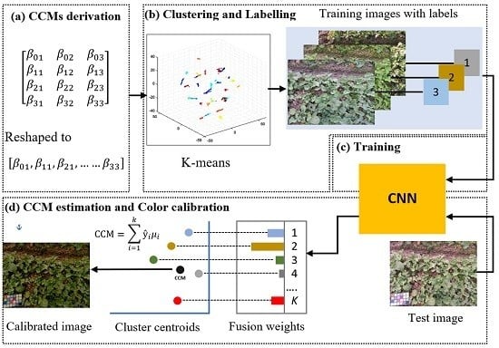
2.2. Overview of the Proposed Method

We proposed to combine the k-means algorithm and deep learning to calibrate the color of our images. Specifically, our proposed framework includes four main steps, as described in Figure 1: (a) the color calibration matrix of each image was firstly computed (ground truth, it should be noted that the manually derived CCM is a ground truth to the final CCM estimated using CNN. The reader should not confuse between this ground truth and standard color values supplied by the X-Rite company.); (b) the training images were categorized based on the color calibration matrix allocated to each image sample; (c) a labeled image dataset was then used to train and validate self-designed deep CNN, and the system was trained to assign scores to a given image to belong to each CCM cluster with some degree of membership; and (d) the CCM of a testing image was calculated by combining the outputs of our deep learning CNN and cluster centroids of the k-means algorithm.

2.2.1. Color Calibration Matrices Derivation

In order to minimize the difference between the standard and measured color values, linear multivariate regression (Equations (1) and (2)) was utilized to regress the average RGB values measured from each color patch (i.e., using the color calibration chart in the acquired image) to the standard color values as suggested by the X-Rite company [42].
S ( R G B ) i = I ( R G B ) i C C M
In expanded form
[ S R 1 S G 1 S B 1 S R 2 S G 2 S B 2 S R n S G n S B n ] = [ 1 I R 1 I G 1 I B 1 1 I R 2 I G 2 I B 2 1 I R n I G n I B 3 ] [ β 01 β 02 β 03 β 11 β 21 β 12 β 22 β 13 β 23 β 31 β 32 β 33 ]
where S and I are standard and measured color values and subscripts R, G, and B are the R-channel, G-channel, and B-channel of RGB color space, respectively. n is the number of color patches, and in our case, there were 24 color patches. The CCMs were represented by the coefficients of the linear multiple regression model. Then the CCM was reshaped to a 1 × 12 row vector as follows (Equation (3)):
[ β 01 , β 11 ,   β 21 ,   β 31 ,   β 02 ,   β 12 , β 22 , β 32 ,   β 03 ,   β 13 ,   β 23 ,   β 33 ]
A total of 3000 CCMs were derived from training and validation image samples (3000 images) and concatenated to form a 3000 × 12 matrix. This matrix was used as the input of the k-means algorithm to provide two outputs, including cluster centers and labels, as described in the next subsection. The CCMs derivation method in this study was modified from work by Shajahan et al. [20]. We derived 4 × 3 CCM that performed both rotation and translation to the color space, which could improve the calibration performance compared with the 3 × 3 CCM that excluded the bias or translation term.

2.2.2. Clustering and Image Labeling

Image clustering is considered as one of the vital steps that improves the performance of the CNN model to estimate the CCMs. In principle, the CNN learns rich features that can best distinguish among different classes [43]. The CNN model is expected to perform more accurately in the cases where classes are well separable as opposed to the cases where the classes are indistinguishable. The CCMs estimation problem falls in the indistinguishable classis’s scenario because images acquired under very similar illumination conditions have similar CCMs. If we directly trained our deep CNN model on this image dataset without grouping, the CNN model might have not been able to distinguish the classes accurately. Therefore, we proposed to first group the images into categories according to the CCM assigned to each image, so as to maximize inter-class differences. This could improve the performance of our CNN model. We employed the k-means algorithm for this purpose. The number of the clusters k was defined using sort of domain knowledge about the illumination variations of our image dataset, which is associated with the number of camera parameters and weather conditions. After the grouping, the labeled images were for training and validation of the deep CNN model.

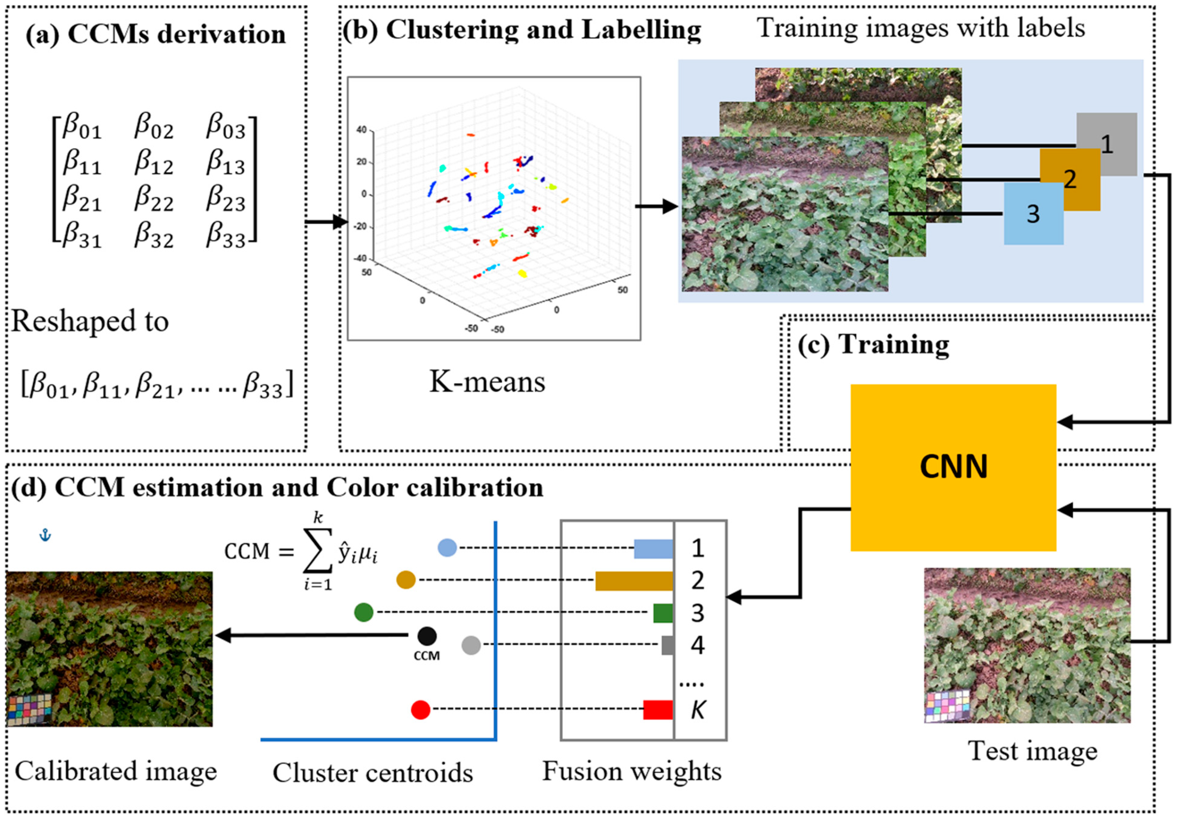
2.2.3. Network Architecture and Training Strategy

After a large number of experiments in which we adjusted the architecture of the network, the sequence of layers was selected taking into account both classification accuracy and training difficulty (see Figure 2 for a graphical representation). The CNN architecture consists of ten convolutional layers (Conv.), two fully-connected (FC) layers, and four max-pooling layers. Each convolution layer is followed by a batch normalization (BN) layer and a rectified linear unit (ReLU) layer. The first FC layer had a 4096 dimensional activation vector and followed by the ReLU layer. The number of output neurons in the final FC layer was set to 30 to be equivalent to the classes used in our study. The softmax layer was stacked at the end to provide probability distribution for the classes (optimal fusion weights). Other hyperparameters of the CNN included filter size, number of filters, and the stride, which were borrowed from the visual geometry group network [35]. We used 3 × 3 receptive fields throughout the network, which were convolved with input at every pixel. The stack of two consecutive 3 × 3 Conv. layers (without spatial pooling in between) had an effective receptive field of 5 × 5, and three such layers had a 7 × 7 effective receptive field, which allowed us to incorporate three ReLU layers instead of a single one and make the decision function more discriminative. By using the small receptive field, the number of parameters can be decreased significantly, and therefore reducing the computation time. Small-size convolution filters have been previously employed by Ciresan et al. [44], but their network is larger than ours. The four max-pooling layers followed some of the Conv. layers instead of all of them, and they were performed over a 2 × 2 pixel window with the stride of 1 × 1. The width of Conv. layers (the number of channels) started from 64 in the first layer and then increased by a factor of two after each max-pooling layer until it reached 512. The number of Conv. layers was decided by fixing the other parameters of the network and steadily increased the depth of the network by adding more convolutional layers until there was no improvement in the validation accuracy. As the network is utilized to provide optimum fusion weights, we placed the softmax layer at the end of the CNN to output a probability distribution over 30 classes [45,46]. The fusion weights were a column vector whose length is equal to k elements and sum to 1. Our final goal of the proposed framework was to compute the CCM, so we should infer the precise CCM from the outputs of the CNN. The estimation procedure of the CCM is described in the following subsection.
Images were resized to 224 × 224 × 3 to match the input of the CNN. During the training of the CNN, the color checker chart was masked out to control its influence on the CNN, and to come up with a model that can describe a real-world application. The CNN model learnable parameters were optimized with the stochastic gradient descent with a momentum of 0.09, a mini-batch size of 66 samples, a learning rate of 0.001, and max epochs of 20. All our modelling framework procedures were conducted in MATLAB 2018a (MathWorks, Inc., Natick, Massachusetts, United States) using deep learning, statistics, machine learning, and computer vision ToolboxTM as a computing software. Our model was run on a graphics processing unit NVIDIA GeForce GTX1080Ti equipped with 3548 compute unified device architecture (CUDA) Cores and 16 GB of graphics processing unit (GPU) memory.

2.2.4. The Network Testing and Image Color Calibration

As already mentioned, our deep CNN was trained to provide the probability (P) of an input image x belonging to one of the k CCM groups. We estimated the CCM of a certain input image from the prediction: ŷ = N(x) using Equation (4).
ŷ = [ P ( y = 1 | x ) P ( y = 2 | x ) P ( y = k | x ) ]
One trivial solution to calculate the CCM is to take the one center of the k-means clusters that corresponds to the highest probability given by the deep CNN model. However, this solution is not suitable for estimating the CCM, because it constrains the possible CCM to only one class. Therefore, we estimated the final CCM by calculating the weighted average of all cluster centers of the k-means (µ) with the fusion weights being P(y = i|x) from the network output following Equation (5), a so-called soft combination method [47,48].
C C M = i = 1 k ŷ i μ i
Using the soft combination method enables our system to estimate the CCM more accurately. As shown in Figure 3, the computed CCM is indicated by a yellow dot, the blue squares show the k-means cluster centers, and the percentage numbers denote the membership scores of a certain image belonging to each CCM class. The CCM was calculated as a weighted average of the cluster centers with the fusion weights being the scores from the deep CNN. The ground truth (GT) is shown as a red diamond. It needs to be mentioned that the 12 length CCM was projected onto a 2D plane in order to obtain a better visualization. This method supposed that the color of the illuminant is spatially unvarying across the image scene. Hence, after the global estimation of the CCM, it can be applied to the uncalibrated image to obtain an image with standard color values. It needs to be mentioned that the standard RGB (sRGB) color space used throughout this work is the linear sRGB color space, in which the gamma-correction was removed.

2.3. Performance Evaluation of the Proposed Framework

The CCM derivation method (4 × 3 CCM) using multivariate linear regression was compared to the method (3 × 3 CCM) proposed by Shajahan et al. [20]. In order to demonstrate the success of the k-means algorithm for accurately differentiating among the image classes based on the CCM assigned to each image, the 12 length CCMs were projected onto a 3D plane using a t-distributed stochastic neighbor embedding (t-SNE) technique [49]. It is a common technique used to reduce non-linear dimensional data. One merit of this technique is that it attempts to preserve the distribution of clusters in the original high-dimensional space when projecting the data into a 3D plane for visualization purposes.
To evaluate the performance of the CNN, a confusion matrix was used to summarize the precision and recall of each class, and the overall accuracy was also computed using Equation (6). We compared the measured color of the uncalibrated image and the standard color on a color reference chart. The color values of the calibrated image were also assessed based on a reference color value. Furthermore, we used Delta_E (ΔΕ) calculated with Equation (7) to measure the color difference among the measured and the reference color values in the international commission on illumination (CIE) 1976 L*a*b* color model. The lower the value of ΔΕ (approach to 1), the more accurate the color calibration is.
O v e R a l l   a c c u R a c y = T P + T N T P + T N + F P + F N
Δ E = 1 24 [ 1 24 ( L 2 * L 1 * ) 2 + ( a 2 * a 1 * ) 2 + ( b 2 * b 1 * ) 2 ]
We also tested the color consistency among images acquired from the same plot under different illumination conditions and used different camera parameter settings. The color intensities of the RGB channels of these images were compared before and after image calibration. Finally, to further confirm the claim considering the progress being made using deep learning methods for image color calibration, the output of our proposed method was compared with previously reported color calibration algorithms, including gray world (GW) [50], principal component analysis (PCA) [51], and white patch (WP) [52]. The comparison was performed using the test dataset (i.e., 150 images). The performance of these algorithms was evaluated by implementing different metrics to describe the error distribution, including mean (µ), median, trimean, best-25% (µ), and worst-25% (µ). In addition to these summarizing statistics, more insight into the performance of the algorithms can be obtained by performing a significant test, like Wilcoxon signed-rank test, which is usually performed between two methods to show that the difference between two algorithms is statistically significant [53].

3. Results and Discussion

In this section, we first demonstrate the improvement being made to the CCM derivation method by comparing it with a method proposed in the literature and then verify the capability of the k-means algorithms for correctly clustering or grouping the images according to the CCM assigned to each image. The classification results of CNN are summarized using a confusion matrix, followed by the evaluation of the CNN training process. The calibration performance of the proposed framework is discussed in two scenarios; in the first scenario, we introduce and discuss the results of the color errors between measured and target colors; while in the second scenario, we demonstrate the color consistency between the calibrated images and discuss its implications for real-world applications. Finally, we prove the claim that using our framework adds considerable enhancement by comparing it with commonly used statistical-based methods in terms of both calibration accuracy and computation time.

3.1. The CCMs Derivation

The CCM derivation is a very critical step in our framework because the CCMs manually derived from whole image samples will finally be combined into one optimal CCM, as described in Section 2.2.4. As depicted in Figure 4, the proposed CCM derivation method reveals that when adding bias or a translation component to the CCM, the color difference between the measured and reference color values was less than 17 ΔΕ, while it was larger than 30 ΔΕ by using 3 × 3 CCM. The color model plays a key role in the color calibration process and can significantly influence the calibration accuracy. This study only used sRGB color space for color calibration, therefore the influence of different color spaces is a topic for future research. Since the digital camera produces non-linearized gamma-corrected images, the linearization of gamma-corrected sRGB color space is an essential step when using sRGB color space with multivariate linear regression. Because the CCM derived by multivariate linear regression only performs a linear transformation, it cannot work well with sRGB color space without removing gamma-correction or linearizing the image. Otherwise, high-order polynomial regression is highly recommended to obtain the mapping coefficient matrix without image linearization [54].

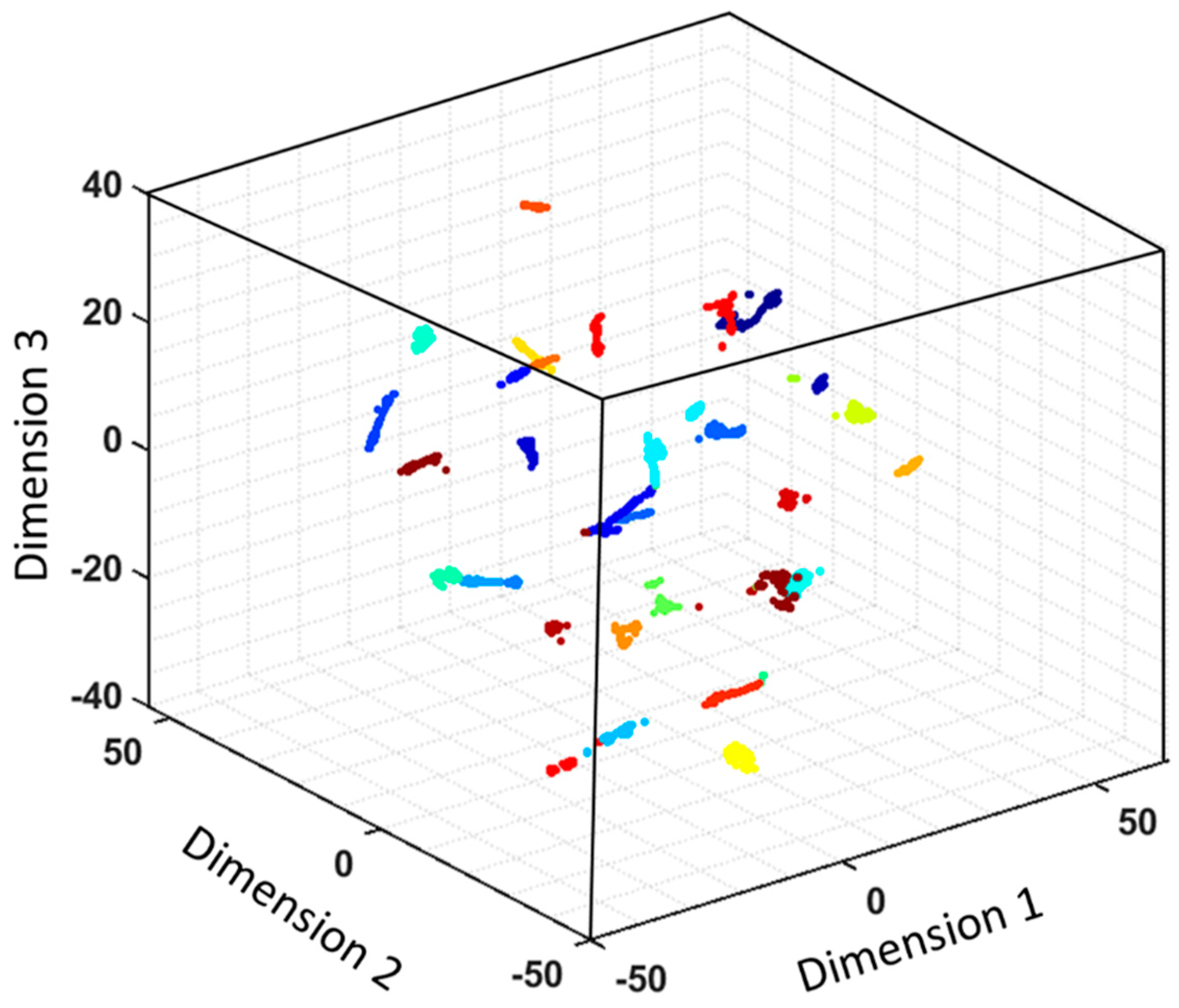
3.2. Performance of the K-Means Clustering

Figure 5 shows the result of the k-means clustering of images based on the CCMs similarity. The classes can be easily discriminated on the 3D space, which reveals that the k-means algorithm can cluster CCMs further apart. We observed that the images acquired under similar illumination conditions often have the same CCM. Therefore, grouping such images together will improve the classification performance of the CNN model. Although many unsupervised learning algorithms (such as the Gaussian mixture model and self-organizing map) can be combined with CNN, the k-means algorithm is simple and more computationally efficient for practical applications [3]. It needs to be mentioned that the optimal number of classes should be carefully selected when combining the k-means algorithm with CNN. When k is small, the training of the deep CNN can be easily performed to classify a test image accurately, but the CCM could not be well estimated from the coarse probability distribution. In contrast, when k is large, the training of CNN becomes difficult, but more accurate CCM can be calculated for correctly classified image samples. Therefore, a trade-off between the complexity of training CNN and final CCM approximation should be considered when selecting k. In our study, the k was selected using some sort of domain knowledge about the variations in the illumination of our image samples, which is associated with the number of camera parameters and variation in the outdoor illumination conditions.

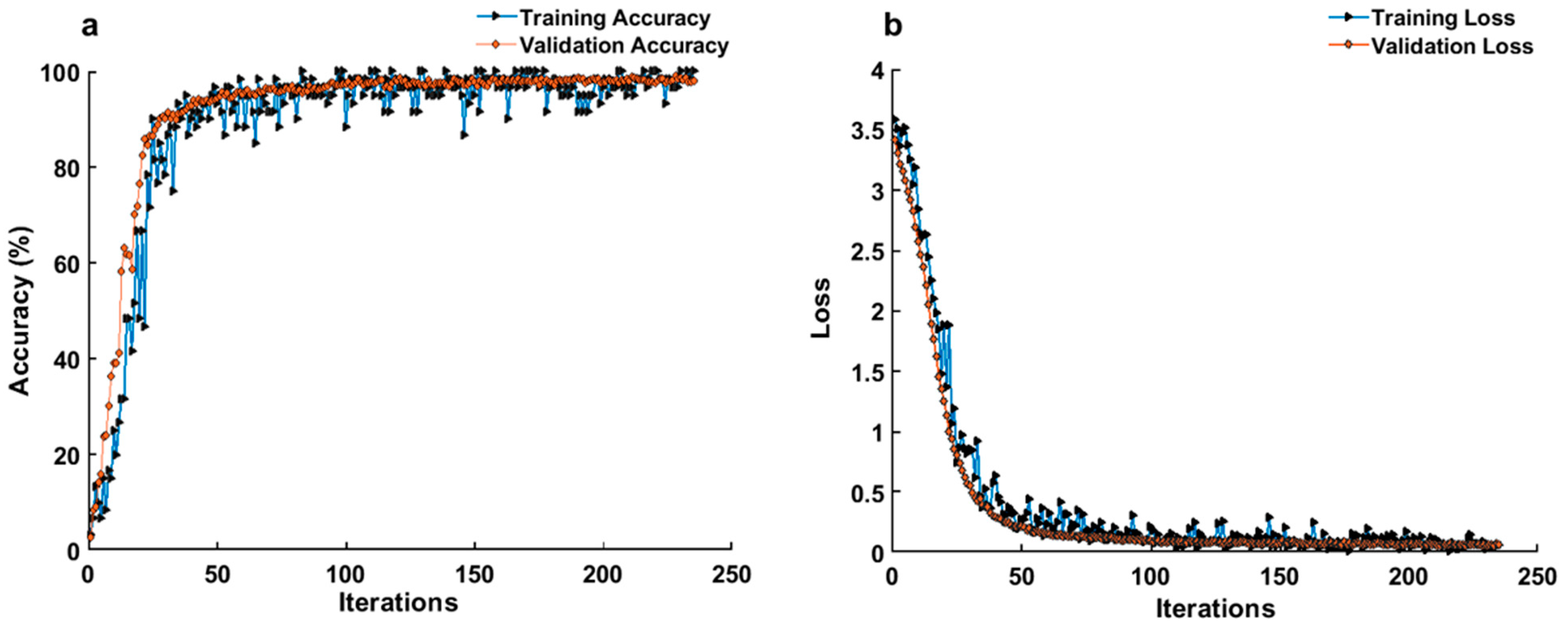
3.3. Performance Evaluation of the CNN Classification

Figure 6 shows the confusion matrix for the CNN classification performance. Our results show that most of the classes were correctly classified with a precision and recall of 100%. Class 17 was partially confused with class 30, which could be due to the similarity between the illumination of two classes.
The CCN model yielded an overall training accuracy of 98.00%, validation accuracy of 98.53 %, and the training time of 2345 minutes, as shown in Table 1. This high training accuracy indicated that the model successfully fit the training dataset. No overfitting problem was observed during the entire training process with a very small difference of 0.53% between the training and the validation accuracies. Besides, the training time was also reasonable since the model only needs to be trained one time. Further, our results showed that the classification was fast enough for real-time applications in the field condition with the classification time of 0.12 s.
Figure 7 shows the training and validation accuracies and losses for each iteration of the training and validation image dataset using the CNN classification model. The training and validation accuracies are gradually improved even after 190 iterations and the training and validation losses more or less established after 150 iterations. This result indicates that CNN has reached the highest accuracy and the lowest loss and did not require any more epochs or iterations. No overfitting problem was observed during the whole training process.

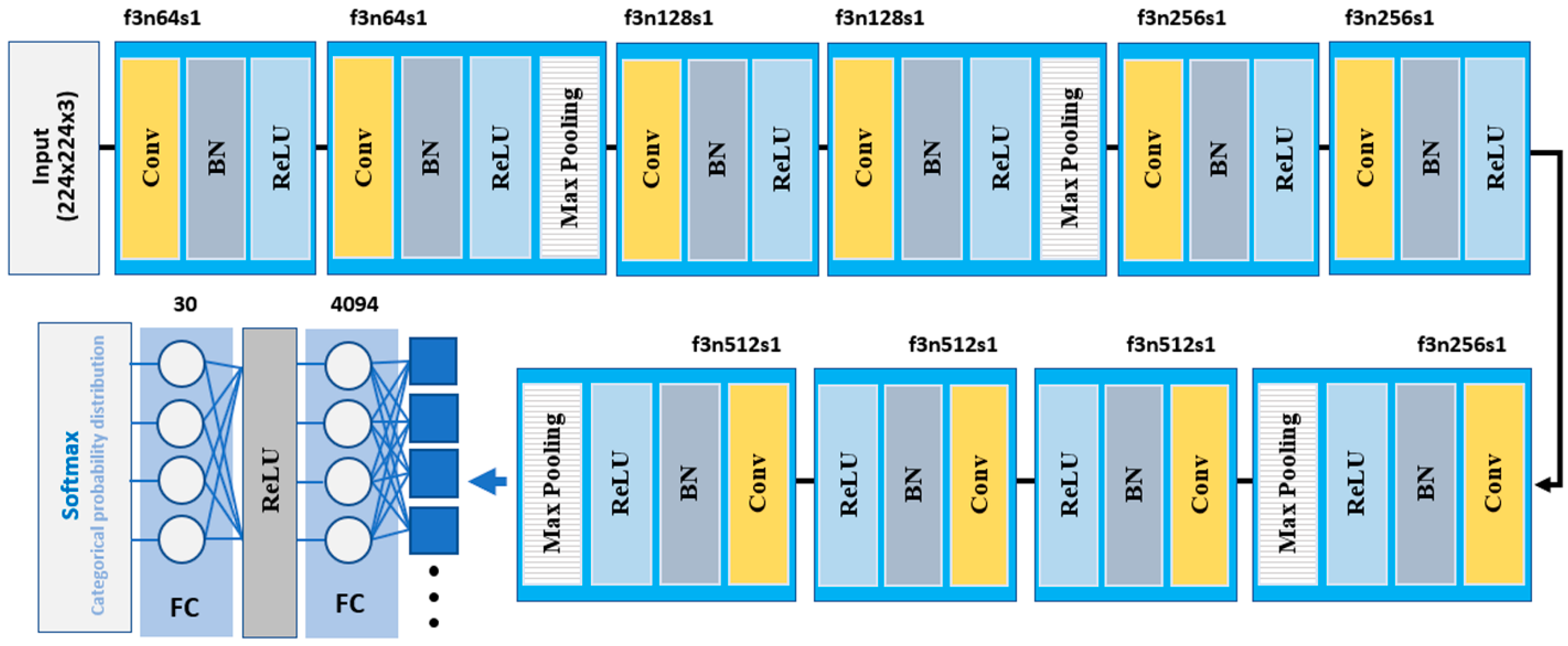
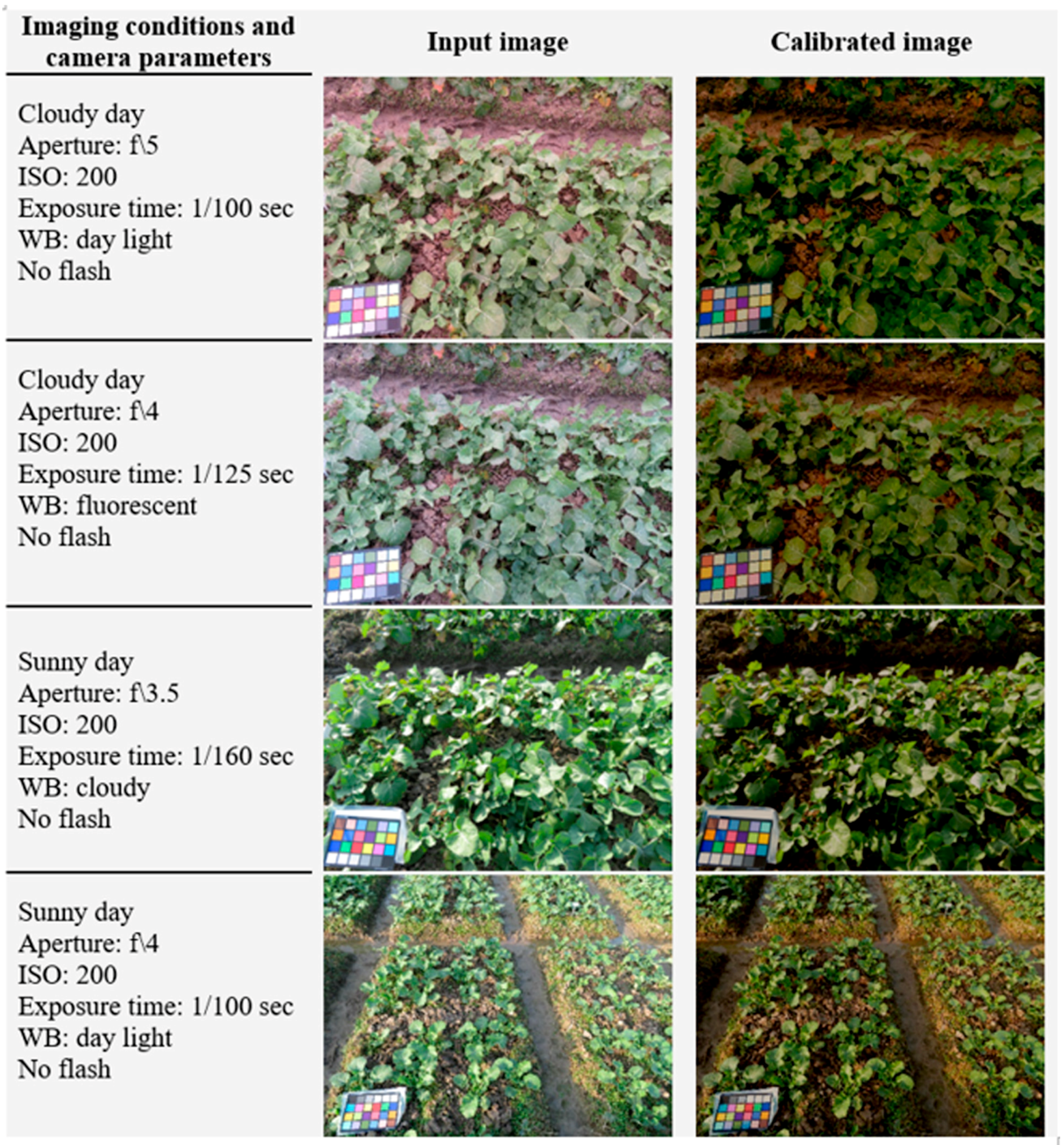
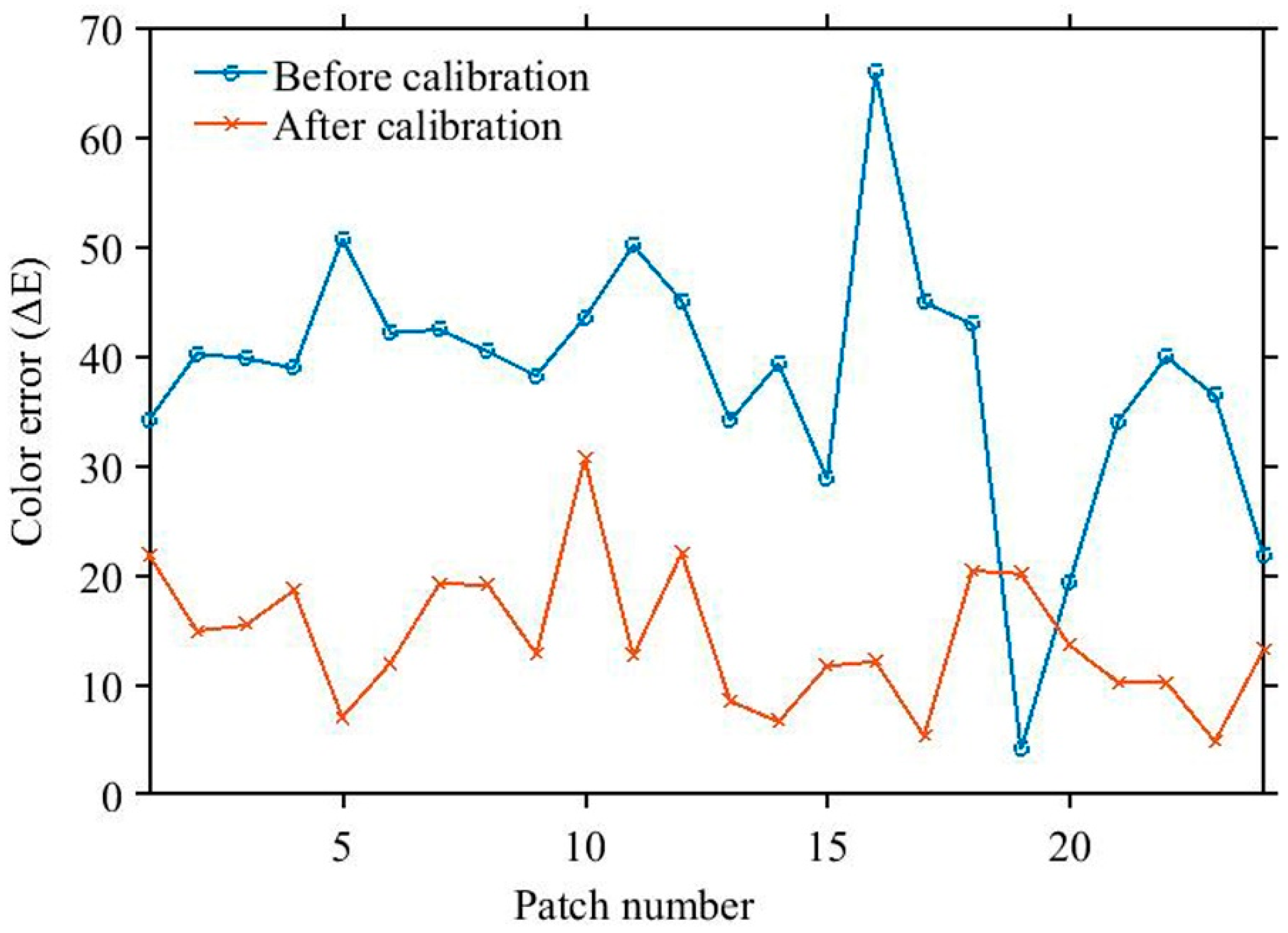
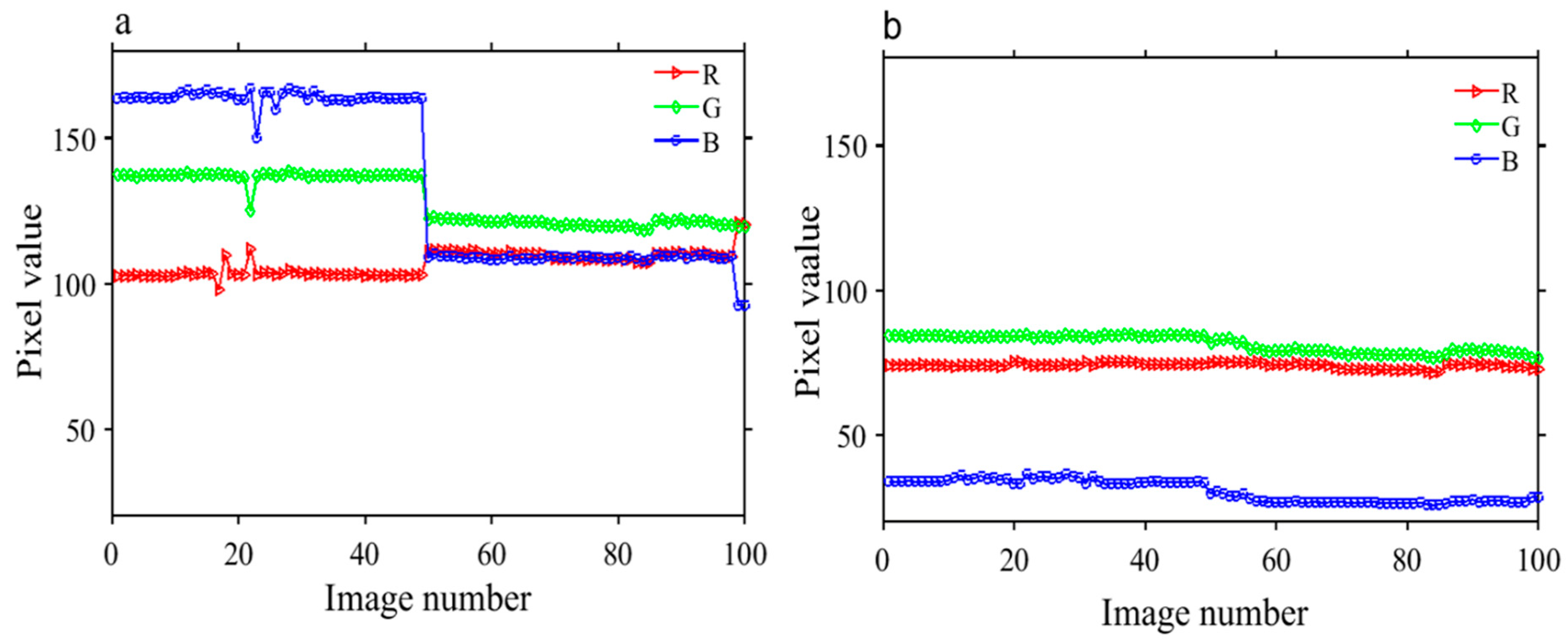
3.4. Performance of Image Color Calibration

In the first column of Figure 8, we showed the imaging conditions and camera parameters as an example of the test images. Because of the different illumination conditions and/or settings of the camera parameters, there was a color inconsistency among images. After applying the color calibration, all the images were turned into a similar color characteristic, as shown in the third column of Figure 8. Based on the visual assessment, it appears reasonable to claim that with using deep learning, the color values of the resulting calibrated images were brought to the reference color values measured under known illuminants.
It is worth mentioning that the color change characteristics of the plant canopy are not only due to variation of illumination conditions, but it is also related to illumination-observation geometries. The plant behaves as an anisotropic reflector that requires characterization of the spectral reflectance (and therefore color) in the different irradiation/viewing directions. Therefore, to account for the effects of illumination and observation directions, it would be better to train the CNN model using images collected from different viewing zenith/azimuth angles.
The quantitative analysis results of the differences between the measured and reference colors before and after the color calibration are presented in Figure 9. It was observed that the measured color errors were smaller for the calibrated image (ranging between 4.9 ΔΕ and 30.70 ΔΕ) than those in the original image (ranging between 4.20 ΔΕ and 66.00 ΔΕ), indicating the colors of the color-corrected image better agreed with the reference colors in most color patches, except in the patch 19 whereby the measured color error of 20.2 ΔΕ was relatively high.
Figure 10 shows mean canopy color in RGB channels for 100 images of a single oilseed rape plot acquired under different illumination conditions using different camera parameter settings. The aim of this figure is not to prove the mean color intensities themselves, but rather to describe the constancy of color measurements over different conditions and varying camera parameter settings. The color before calibration implies too severe changes in color to be associated with a biological phenomenon, as shown in Figure 10a. Although all images were collected from the same plot, the mean color intensities varied among image sessions due to the different illumination conditions and camera parameter settings. While the intensity remained more consistent after the color calibration, as presented in Figure 10b. It was also noted that the color corrected images had consistently higher green intensity than red and blue due to the high chlorophyll content at the seedling stage. While at the senescence stage, the red value is expected to be increased, as plants begin to turn yellow with decreased chlorophyll content (data was not shown here) [55]. It would be very difficult to observe such chlorophyll-related changing patterns of plants from RGB images without color calibration.
Our study focused on improving the efficiency of the color calibration process using a deep learning-based method and demonstrating its applicability in real-time series data and did not consider its implications and usefulness for typical plant phenotyping analyses since this was demonstrated in several studies [55,56]. For example, color-corrected images are useful for detecting the variations among different plant varieties or plants grown under different nitrogen concentrations, and even plants grown under inconsistent illumination conditions [57]. Also, studies have used color-corrected images to detect the senescence stage of the crops [58]. In this context, our color-corrected images could be employed to estimate oilseed rape phenotypic traits, such as yield, biomass, and chlorophyll content.

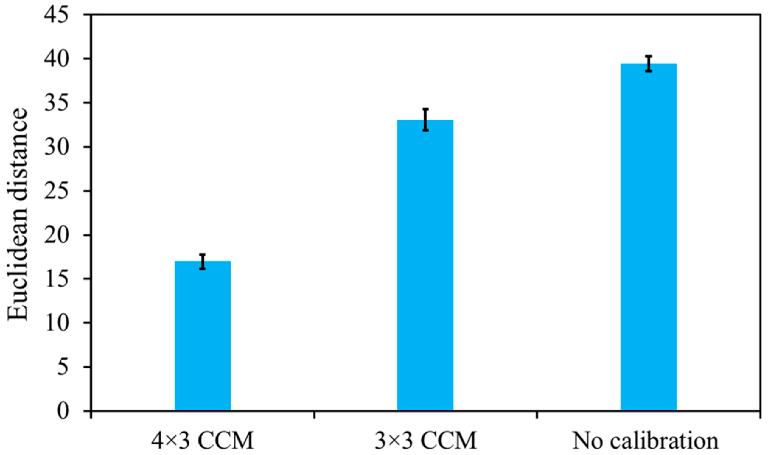
3.5. Comparison of Different Color Calibration Methods

Table 2 shows the comparison between our proposed color calibration method and the previously reported algorithms like GW, WP, and PCA, and the statistical significance by Wilcoxon signed-rank test is presented in Table 3. Although GW, WP, and PCA were fast enough in the color calibration process, their calibration errors were high. The average color errors using these methods range between 35 ΔΕ and 38 ΔΕ. While our proposed framework achieved the best performance with an accuracy of 16.23 ΔΕ, which is significantly lower than GW, WP, and PCA algorithms, the time is comparably longer than GW, WP, and PCA methods. The processing time of color calibration using GW, WP, and PCA was fast because these algorithms calibrated the color by simply scaling the color value of each pixel with a certain constant. While our calibration method was performed by using multiple steps, including classification, CCM estimation, and color correction, which takes a little bit longer but is still acceptable for real-time applications as suggested by Bosilj et al. [59], our future work will focus on improving the computation time by further reducing the learnable parameters of the CNN architecture while keeping the same level of the calibration accuracy.

4. Conclusions

In this study, we proposed an efficient deep learning framework combined with the k-means algorithm for calibrating the color of oilseed rape images. We demonstrated the potential of deep CNN for extraction of low-level features (e.g., color of the illuminant) to discriminate between images collected under different illumination conditions and using various camera parameter settings. The deep learning model achieved overall training and validation accuracies of 98.00% and 98.53%, respectively. The output of the deep CNN combined with k-means cluster centers estimated the CCM automatically. Our proposed approach outperformed previously reported methods with a mean color error of 16.23 ΔΕ, and the deep learning framework showed superior performance for rapidly calibrating images in an automated fashion in a relatively short time of 0.15 s. The proposed framework can be incorporated with any aerial- or ground-based platforms for accurately performing color calibration of RGB images to characterize the phenotypic traits of the plant consistently. Future work will be focused on exploring the capability of unsupervised deep learning methods, using a more comprehensive dataset from different crops under controlled and natural conditions, and performing color calibration on a per pixel-level.

Author Contributions

All authors made significant contributions to this paper. A.A. and H.C. developed the main idea of this manuscript. A.A. designed the experiment, collected the data from field, and performed the data analysis and was the main author of this paper. A.A. and L.W. wrote the paper. K.M, E.A.-R., and Y.H. reviewed the paper. All authors read and approved the manuscript.

Funding

This research was supported by the National Natural Science Foundation of China (31801256), and National Key R&D Program of China (2017YFD0201501).

Conflicts of Interest

The authors declare no conflict of interest.

References

  1. Zhang, J.; Naik, H.S.; Assefa, T.; Sarkar, S.; Reddy, R.C.; Singh, A.; Ganapathysubramanian, B.; Singh, A.K. Computer vision and machine learning for robust phenotyping in genome-wide studies. Sci. Rep. 2017, 7, 44048. [Google Scholar] [CrossRef] [PubMed]
  2. Sulistyo, S.B.; Wu, D.; Woo, W.L.; Dlay, S.S.; Gao, B. Computational deep intelligence vision sensing for nutrient content estimation in agricultural automation. IEEE Trans. Autom. Sci. Eng. 2017, 15, 1243–1257. [Google Scholar] [CrossRef]
  3. Abdalla, A.; Cen, H.; El-manawy, A.; He, Y. Infield oilseed rape images segmentation via improved unsupervised learning models combined with supreme color features. Comput. Electron. Agric. 2019. [Google Scholar] [CrossRef]
  4. Furbank, R.T.; Tester, M. Phenomics—Technologies to relieve the phenotyping bottleneck. Trends Plant Sci. 2011, 16, 635–644. [Google Scholar] [CrossRef]
  5. Rahaman, M.M.; Chen, D.; Gillani, Z.; Klukas, C.; Chen, M. Advanced phenotyping and phenotype data analysis for the study of plant growth and development. Front. Plant Sci. 2015, 6, 619. [Google Scholar] [CrossRef] [Green Version]
  6. Chen, D.; Neumann, K.; Friedel, S.; Kilian, B.; Chen, M.; Altmann, T.; Klukas, C. Dissecting the Phenotypic Components of Crop Plant Growth and Drought Responses Based on High-Throughput Image Analysis. Plant Cell 2014. [Google Scholar] [CrossRef] [Green Version]
  7. Hernández-Hernández, J.L.; García-Mateos, G.; González-Esquiva, J.M.; Escarabajal-Henarejos, D.; Ruiz-Canales, A.; Molina-Martínez, J.M. Optimal color space selection method for plant/soil segmentation in agriculture. Comput. Electron. Agric. 2016, 122, 124–132. [Google Scholar] [CrossRef]
  8. Guo, W.; Rage, U.K.; Ninomiya, S. Illumination invariant segmentation of vegetation for time series wheat images based on decision tree model. Comput. Electron. Agric. 2013, 96, 58–66. [Google Scholar] [CrossRef]
  9. Barbedo, J.G.A. A review on the main challenges in automatic plant disease identification based on visible range images. Biosys. Eng. 2016, 144, 52–60. [Google Scholar] [CrossRef]
  10. Liang, Y.; Urano, D.; Liao, K.-L.; Hedrick, T.L.; Gao, Y.; Jones, A.M.J.P.M. A nondestructive method to estimate the chlorophyll content of Arabidopsis seedlings. Plant Methods 2017, 13, 26. [Google Scholar] [CrossRef]
  11. Riccardi, M.; Mele, G.; Pulvento, C.; Lavini, A.; d’Andria, R.; Jacobsen, S.-E.J.P.R. Non-destructive evaluation of chlorophyll content in quinoa and amaranth leaves by simple and multiple regression analysis of RGB image components. Photosynth. Res. 2014, 120, 263–272. [Google Scholar] [CrossRef]
  12. Jiménez-Zamora, A.; Delgado-Andrade, C.; Rufián-Henares, J.A. Antioxidant capacity, total phenols and color profile during the storage of selected plants used for infusion. Food Chem. 2016, 199, 339–346. [Google Scholar] [CrossRef]
  13. Esaias, W.E.; Iverson, R.L.; Turpie, K. Ocean province classification using ocean colour data: Observing biological signatures of variations in physical dynamics. Glob. Chang. Biol. 2000, 6, 39–55. [Google Scholar] [CrossRef]
  14. Malmer, N.; Johansson, T.; Olsrud, M.; Christensen, T.R. Vegetation, climatic changes and net carbon sequestration in a North-Scandinavian subarctic mire over 30 years. Global Change Biol. 2005, 11, 1895–1909. [Google Scholar] [CrossRef]
  15. Grose, M.J. Green leaf colours in a suburban Australian hotspot: Colour differences exist between exotic trees from far afield compared with local species. Landsc. Urban Plan. 2016, 146, 20–28. [Google Scholar] [CrossRef]
  16. Grose, M.J. Plant colour as a visual aspect of biological conservation. Biol. Conserv. 2012, 153, 159–163. [Google Scholar] [CrossRef]
  17. Porikli, F. Inter-camera color calibration by correlation model function. In Proceedings of the 2003 International Conference on Image Processing (Cat. No.03CH37429), Barcelona, Spain, 14–17 September 2003; p. II-133. [Google Scholar]
  18. Brown, M.; Majumder, A.; Yang, R. Camera-based calibration techniques for seamless multiprojector displays. IEEE Trans. Vis. Comput. Graph. 2005, 11, 193–206. [Google Scholar] [CrossRef]
  19. Kagarlitsky, S.; Moses, Y.; Hel-Or, Y. Piecewise-consistent Color Mappings of Images Acquired Under Various Conditions; IEEE: Piscataway, NJ, USA, 2009; pp. 2311–2318. [Google Scholar]
  20. Shajahan, S.; Igathinathane, C.; Saliendra, N.; Hendrickson, J.R.; Archer, D. Color calibration of digital images for agriculture and other applications. ISPRS J. Photogram. Remote Sens. 2018, 146, 221–234. [Google Scholar]
  21. Charrière, R.; Hébert, M.; Treméau, A.; Destouches, N. Color calibration of an RGB camera mounted in front of a microscope with strong color distortion. Appl. Opt. 2013, 52, 5262–5271. [Google Scholar]
  22. Finlayson, G.; Mackiewicz, M.; Hurlbert, A. Color Correction Using Root-Polynomial Regression. IEEE Trans. Image Process 2015, 24, 1460–1470. [Google Scholar] [CrossRef] [Green Version]
  23. Jetsu, T.; Heikkinen, V.; Parkkinen, J.; Hauta-Kasari, M.; Martinkauppi, B.; Lee, S.D.; Ok, H.W.; Kim, C.Y. Color calibration of digital camera using polynomial transformation. In Proceedings of the Conference on Colour in Graphics, Imaging, and Vision, Leeds, UK, 19–22 June 2006; pp. 163–166. [Google Scholar]
  24. Jackman, P.; Sun, D.-W.; ElMasry, G. Robust colour calibration of an imaging system using a colour space transform and advanced regression modelling. Meat Sci. 2012, 91, 402–407. [Google Scholar] [CrossRef] [PubMed]
  25. Kang, H.R.; Anderson, P. Neural network applications to the color scanner and printer calibrations. J. Electron. Imaging 1992, 1, 125–135. [Google Scholar]
  26. Wee, A.G.; Lindsey, D.T.; Kuo, S.; Johnston, W.M. Color accuracy of commercial digital cameras for use in dentistry. Dent. Mater. 2006, 22, 553–559. [Google Scholar] [CrossRef] [PubMed]
  27. Colantoni, P.; Thomas, J.-B.; Yngve Hardeberg, J. High-end colorimetric display characterization using an adaptive training set. J. Soc. Inf. Disp. 2011, 19, 520–530. [Google Scholar] [CrossRef] [Green Version]
  28. Chen, C.-L.; Lin, S.-H. Intelligent color temperature estimation using fuzzy neural network with application to automatic white balance. Expert Syst. Appl. 2011, 38, 7718–7728. [Google Scholar] [CrossRef]
  29. Bala, R.; Monga, V.; Sharma, G.; R. Van de Capelle, J.-P. Two-dimensional transforms for device color calibration. Proc. SPIE 2003, 5293. [Google Scholar]
  30. Virgen-Navarro, L.; Herrera-López, E.J.; Corona-González, R.I.; Arriola-Guevara, E.; Guatemala-Morales, G.M. Neuro-fuzzy model based on digital images for the monitoring of coffee bean color during roasting in a spouted bed. Expert Syst. Appl. 2016, 54, 162–169. [Google Scholar] [CrossRef]
  31. Akkaynak, D.; Treibitz, T.; Xiao, B.; Gürkan, U.A.; Allen, J.J.; Demirci, U.; Hanlon, R.T. Use of commercial off-the-shelf digital cameras for scientific data acquisition and scene-specific color calibration. J. Opt. Soc. Am. A 2014, 31, 312–321. [Google Scholar] [CrossRef] [Green Version]
  32. Suh, H.K.; Ijsselmuiden, J.; Hofstee, J.W.; van Henten, E.J. Transfer learning for the classification of sugar beet and volunteer potato under field conditions. Biosys. Eng. 2018, 174, 50–65. [Google Scholar] [CrossRef]
  33. Krizhevsky, A.; Sutskever, I.; E. Hinton, G. ImageNet Classification with Deep Convolutional Neural Networks. In Proceedings of the 25th International Conference on Neural Information Processing Systems, Lake Tahoe, Nevada, 3–6 December 2012; Volume 25. [Google Scholar]
  34. Girshick, R.; Donahue, J.; Darrell, T.; Malik, J. Rich Feature Hierarchies for Accurate Object Detection and Semantic Segmentation. In Proceedings of the 2014 IEEE Conference on Computer Vision and Pattern Recognition, Washington, DC, USA, 23–28 June 2014; pp. 580–587. [Google Scholar]
  35. Simonyan, K.; Zisserman, A. Very Deep Convolutional Networks for Large-Scale Image Recognition. arXiv 2014, arXiv:1409.1556. [Google Scholar]
  36. Bay, H.; Ess, A.; Tuytelaars, T.; Van Gool, L. Speeded-Up Robust Features (SURF). Comput. Vision Image Understanding 2008, 110, 346–359. [Google Scholar] [CrossRef]
  37. Lowe, D.G. Object recognition from local scale-invariant features. In Proceedings of the Seventh IEEE International Conference on Computer Vision, Kerkyra, Greece, 20–27 September 1999; Volume 1152, pp. 1150–1157. [Google Scholar]
  38. Shi, W.; Loy, C.C.; Tang, X. Deep Specialized Network for Illuminant Estimation. In Proceedings of the Computer Vision—ECCV 2016, Cham, The Netherlands, 8–16 October 2016; pp. 371–387. [Google Scholar]
  39. Lou, Z.; Gevers, T.; Hu, N.; Lucassen, M. Color Constancy by Deep Learning. In Proceedings of the British Machine Vision Conference, Swansea, UK, 7–10 September 2015; pp. 76.1–76.12. [Google Scholar] [CrossRef] [Green Version]
  40. Qian, Y.; Chen, K.; Kamarainen, J.-K.; Nikkanen, J.; Matas, J. Deep Structured-Output Regression Learning for Computational Color Constancy. In Proceedings of the 2016 23rd International Conference on Pattern Recognition (ICPR), Cancun, Mexico, 4–8 December 2016. [Google Scholar]
  41. Gong, R.; Wang, Q.; Shao, X.; Liu, J. A color calibration method between different digital cameras. Optik 2016, 127, 3281–3285. [Google Scholar] [CrossRef]
  42. X-Rite. Colorimetric values for ColorChecker Family of Targets. Available online: https://xritephoto.com/ph_product_overview.aspx?ID=1257&Action=Support&SupportID=5159 (accessed on 11 February 2018).
  43. Oh, S.W.; Kim, S.J. Approaching the computational color constancy as a classification problem through deep learning. Pattern Recognit. 2017, 61, 405–416. [Google Scholar] [CrossRef] [Green Version]
  44. Ciresan, D.C.; Meier, U.; Masci, J.; Gambardella, L.M.; Schmidhuber, J. Flexible, high performance convolutional neural networks for image classification. In Proceedings of the Twenty-Second International Joint Conference on Artificial Intelligence, Catalonia, Spain, 16–22 July 2011. [Google Scholar]
  45. Krizhevsky, A.; Sutskever, I.; Hinton, G.E. ImageNet classification with deep convolutional neural networks. J. Commun. ACM 2017, 60, 84–90. [Google Scholar] [CrossRef]
  46. Bridle, J.S. Probabilistic Interpretation of Feedforward Classification Network Outputs, with Relationships to Statistical Pattern Recognition; Springer: Berlin/Heidelberg, Germany, 1990; pp. 227–236. [Google Scholar]
  47. Bianco, S.; Gasparini, F.; Schettini, R. Consensus-based framework for illuminant chromaticity estimation. J. Electron. Imaging 2008, 17, 023013. [Google Scholar] [CrossRef] [Green Version]
  48. Gijsenij, A.; Gevers, T.; Weijer, J.v.d. Computational Color Constancy: Survey and Experiments. IEEE Trans. Image Process. 2011, 20, 2475–2489. [Google Scholar] [CrossRef]
  49. Maaten, L.v.d.; Hinton, G. Visualizing data using t-SNE. J. Mach. Learn. Res. 2008, 9, 2579–2605. [Google Scholar]
  50. Buchsbaum, G. A spatial processor model for object colour perception. J. Frankl. Inst. 1980, 310, 1–26. [Google Scholar] [CrossRef]
  51. Cheng, D.; Prasad, D.K.; Brown, M.S. Illuminant estimation for color constancy: Why spatial-domain methods work and the role of the color distribution. J. Opt. Soc. Am. A 2014, 31, 1049–1058. [Google Scholar] [CrossRef]
  52. Land, E.H.; McCann, J.J. Lightness and Retinex Theory. J. Opt. Soc. Am. 1971, 61, 1–11. [Google Scholar] [CrossRef] [PubMed]
  53. Gijsenij, A.; Gevers, T.; Lucassen, M.P. Perceptual analysis of distance measures for color constancy algorithms. JOSA A 2009, 26, 2243–2256. [Google Scholar] [CrossRef] [PubMed] [Green Version]
  54. Zhu, Z.; Song, R.; Luo, H.; Xu, J.; Chen, S. Color Calibration for Colorized Vision System with Digital Sensor and LED Array Illuminator. Act. Passiv. Electron. Compon. 2016, 2016. [Google Scholar] [CrossRef] [Green Version]
  55. Chopin, J.; Kumar, P.; Miklavcic, S. Land-based crop phenotyping by image analysis: Consistent canopy characterization from inconsistent field illumination. Plant Methods 2018, 14, 39. [Google Scholar] [CrossRef] [PubMed]
  56. Grieder, C.; Hund, A.; Walter, A. Image based phenotyping during winter: A powerful tool to assess wheat genetic variation in growth response to temperature. Funct. Plant Biol. 2015, 42, 387. [Google Scholar] [CrossRef]
  57. Buchaillot, M.; Gracia Romero, A.; Vergara, O.; Zaman-Allah, M.; Tarekegne, A.; Cairns, J.; M Prasanna, B.; Araus, J.; Kefauver, S. Evaluating Maize Genotype Performance under Low Nitrogen Conditions Using RGB UAV Phenotyping Techniques. Sensors 2019, 19, 1815. [Google Scholar] [CrossRef] [Green Version]
  58. Makanza, R.; Zaman-Allah, M.; Cairns, J.; Magorokosho, C.; Tarekegne, A.; Olsen, M.; Prasanna, B. High-Throughput Phenotyping of Canopy Cover and Senescence in Maize Field Trials Using Aerial Digital Canopy Imaging. Remote Sens. 2018, 10, 330. [Google Scholar] [CrossRef] [Green Version]
  59. Bosilj, P.; Aptoula, E.; Duckett, T.; Cielniak, G. Transfer learning between crop types for semantic segmentation of crops versus weeds in precision agriculture. J. Field Robot 2019. [Google Scholar] [CrossRef]
Figure 1. Flowchart of the proposed color calibration framework. CCM: color calibration matrix; CNN: convolutional neural network.
Remotesensing 11 03001 g001
Figure 2. The architecture of our deep learning convolutional neural network (CNN). f, n, and s represent the filter size, number of filters, and stride for each convolutional layer, respectively.
Remotesensing 11 03001 g002
Figure 3. An example of a corrected image (a) and its computed color calibration matrix as indicated by a yellow dot (b).
Remotesensing 11 03001 g003
Figure 4. Comparison of different color calibration matrices derivation methods. The x-axis shows the average Euclidean distance between standard and measured colors of 24 patches.
Remotesensing 11 03001 g004
Figure 5. A t-distributed stochastic neighbor embedding (t-SNE) visualization of color calibration matrices (CCMs) corresponding to the images collected from the field. Each color represents a different class in the datasets. Note that the CCMs belonging to the same class were grouped.
Remotesensing 11 03001 g005
Figure 6. Confusion matrix for the convolutional neural network (CNN) classification experiment using the validation dataset. The precision and recall for each class were presented using column and row summaries.
Remotesensing 11 03001 g006
Figure 7. Training and validation accuracies (a) and losses (b) of each iteration of the training and validation processes of the convolutional neural network (CNN) classification algorithm.
Remotesensing 11 03001 g007
Figure 8. Visual assessment of image color calibration using the proposed framework. WB: white balance, ISO: international organization of standardization.
Remotesensing 11 03001 g008
Figure 9. The color difference between the measured and target color of 24 patches before and after color calibration. ΔΕ represents the Euclidean distance between measured and target colors in the international commission on illumination (CIE) 1976 L*a*b* color model. For an easy interpretation of the color references in this figure legend, the reader is referred to the online version of this article.
Remotesensing 11 03001 g009
Figure 10. Mean canopy color under varying illumination conditions and using different camera settings. Mean canopy color values in red (R), green (G), and blue (B) of the 100 images before (a) and after (b) color calibration for a single oilseed rape plot.
Remotesensing 11 03001 g010
Table 1. Overall accuracies of the convolutional neural network (CNN) for training and validation images. Note that classification time denotes the time needed to classify one image and does not include the time needed for color calibration. The training time is the time required to train the entire network from scratch over 20 epochs, and no stopping criterion was used.
Training No. of ImagesValidation No. of ImagesTraining Time (min)Classification Time (s/Image)Training Accuracy (%)Validation Accuracy (%)
210090023450.1298.0098.53
Table 2. Comparison of the performance of different image color calibration algorithms, including our proposed framework, grey world (GW), white patch (WP), and principal component analysis (PCA). The algorithm with the best performance is highlighted in bold. N/A = not available.
MethodMean (µ)MedianTrimeanBest-25% (µ)Worst-25% (µ)Time (s)
No calibration41.9440.3942.5838.2546.28N/A
Proposed method16.2313.2714.8510.9223.370.150
GW35.0933.7234.1827.9342.980.132
WP38.9736.0937.9434.3944.470.112
PCA35.4633.8534.7229.1142.230.146
Table 3. Wilcoxon signed-rank test compared the performance difference of each two methods. A positive value (1) at the location (i,j) indicates the median of the method i is significantly lower than the median of method j at the 95% confidence level. A negative value (−1) indicates the opposite and zero (0) indicates there is no significant difference between the two methods.
PCAWPGWProposed
1110Proposed
110−1GW
−10−1−1WP
01−1−1PCA

