Leveraging Very-High Spatial Resolution Hyperspectral and Thermal UAV Imageries for Characterizing Diurnal Indicators of Grapevine Physiology

Abstract

Efficient and accurate methods to monitor crop physiological responses help growers better understand crop physiology and improve crop productivity. In recent years, developments in unmanned aerial vehicles (UAV) and sensor technology have enabled image acquisition at very-high spectral, spatial, and temporal resolutions. However, potential applications and limitations of very-high-resolution (VHR) hyperspectral and thermal UAV imaging for characterization of plant diurnal physiology remain largely unknown, due to issues related to shadow and canopy heterogeneity. In this study, we propose a canopy zone-weighting (CZW) method to leverage the potential of VHR (≤9 cm) hyperspectral and thermal UAV imageries in estimating physiological indicators, such as stomatal conductance (G_s) and steady-state fluorescence (F_s). Diurnal flights and concurrent in-situ measurements were conducted during grapevine growing seasons in 2017 and 2018 in a vineyard in Missouri, USA. We used neural net classifier and the Canny edge detection method to extract pure vine canopy from the hyperspectral and thermal images, respectively. Then, the vine canopy was segmented into three canopy zones (sunlit, nadir, and shaded) using K-means clustering based on the canopy shadow fraction and canopy temperature. Common reflectance-based spectral indices, sun-induced chlorophyll fluorescence (SIF), and simplified canopy water stress index (siCWSI) were computed as image retrievals. Using the coefficient of determination (R²) established between the image retrievals from three canopy zones and the in-situ measurements as a weight factor, weighted image retrievals were calculated and their correlation with in-situ measurements was explored. The results showed that the most frequent and the highest correlations were found for G_s and F_s, with CZW-based Photochemical reflectance index (PRI), SIF, and siCWSI (PRI_CZW, SIF_CZW, and siCWSI_CZW), respectively. When all flights combined for the given field campaign date, PRI_CZW, SIF_CZW, and siCWSI_CZW significantly improved the relationship with G_s and F_s. The proposed approach takes full advantage of VHR hyperspectral and thermal UAV imageries, and suggests that the CZW method is simple yet effective in estimating G_s and F_s.

1. Introduction

Grapevine (Vitis spp.) is one of the most commercially important berry crops in the world [1]. In grapevines, moderate water deficit is necessary to achieve desired berry quality and yield, although the effects of deficit irrigation on berry and quality are dependent upon the weather during the growing season, soil type, grapevine variety, and timing of water application [2,3,4,5]. Understanding the physiological responses of grapevine to mild to moderate water stress is fundamental to optimize deficit irrigation timing and amount [5,6]. Additionally, vine physiology is sensitive to diurnal cycles and vineyard microclimates, with even temporary stress having the potential to alter berry chemistry and vine growth [7,8]. Therefore, it is critical to account for physiological changes associated with these factors in field conditions throughout diurnal cycles rather than focusing only on pre-dawn or midday measurements, which are often used [5,6].

Current methods for estimating physiological processes include quantification of gas exchange, stomatal conductance, canopy temperature, and stem water potential [9]. These approaches are time-consuming, labor-intensive, and destructive (leaves need to be detached for stem water potential). Further, they are unsuitable for automation, subject to measurement and sampling errors, and the instrumentation required can be prohibitive in terms of cost [10,11]. More importantly, the data collected with traditional tools represent incomplete spatial and temporal characterization of key vine physiological parameters due to the time involved in taking the measurements and the capacity of the instruments themselves [12,13]. Therefore, it is necessary to have efficient monitoring systems that enable accurate tracking of key parameters governing vine function at high spatial and temporal resolution to obtain a reliable overview of vine physiology.

Hyperspectral and thermal sensors installed on field robots-, aircraft-, and satellite-based platforms are an increasingly common approach used to characterize plant physiology [14,15,16,17]. In hyperspectral remote sensing, sensors measure radiative properties of plants with hundreds to thousands of continuous narrow bands in the optical domain (0.35–2.5 µm). This abundant spectral information increases the chance of detecting subtle physiological changes compared to multispectral data, which have a small number of bands averaged over a wide spectral region and are insensitive to narrow spectral signatures [18,19,20]. Photochemical reflectance index (PRI) and sun-induced fluorescence (SIF) retrieved from hyperspectral remote sensing are the most widely used indicators in the remote assessment of plant photosynthetic activity [21,22,23,24]. The PRI was formed to track the xanthophyll cycle, which relates to plant oxidative stress associated with photosynthesis, using changes in green reflectance centered at 531 nm [25]. SIF is a direct proxy of photosynthesis, because it detects reemitted excess light energy at 600–800 nm, from photosystems I and II, to minimize photosystem damage as a part of the plant photo-protective mechanism [26,27,28,29].

Thermal remote sensing (8–14 µm) is a popular tool but unlike the aforementioned indices that rely on factors related to photosynthetic activity, thermal data is a strong proxy for transpiration activity. Therefore, the rationale behind the application of thermal remote sensing for plant stress detection is the correlation between stress level and plant temperature increase, which is triggered by stomatal closure and reduced transpiration [30]. To overcome the effects of varying meteorological conditions on the stress and temperature relationship, the canopy water stress index (CWSI) was developed by the normalizing canopy (T_c) and air temperate (T_a) difference with the evaporative demand [31,32].

When satellite- or aircraft-based hyperspectral and thermal observations are made, the above-mentioned remotely sensed indices are affected by many factors, including soil/background, canopy architecture, and shadow due to the lack of spatial resolution [17,33,34,35,36]. This is particularly true for highly heterogeneous fields of perennial woody crops (e.g., orchard and vineyards), where plants are planted in rows with cover crops or bare soil between the rows [15,37,38]. Further, low revisit frequency, high cost, and potential cloud occurrence limit the suitability of satellite remote sensing in agriculture, while operational complexity presents a major constraint for manned airborne platforms [39,40,41]. Alternatively, remotely sensed data from field-based platforms (poles/towers and manned/unmanned vehicles) have the capacity to assess plant health status [42,43]. However, there are shortcomings in these as well, such as that field-based remote sensing platforms are not easily transported and often offer a limited footprint [44,45,46].

Within the past few years, huge strides have been made in unmanned aerial vehicles (UAVs) and sensor technologies, which have enabled image acquisition at high spectral, spatial, and temporal resolutions over small to medium fields. Inexpensive and agile UAVs equipped with lightweight miniaturized sensors offer attractive alternatives for field-scale phenotyping and precision agriculture [44,47,48]. However, UAV-based studies have been limited by cost, experienced pilot shortages, lack of methods for fast data processing, and strict airspace regulations [44]. With the availability of lower-cost commercial UAV platforms (which are easy to operate) and sensors, improved image processing methods, and effective airspace regulations, those limitations are becoming less relevant [44,49,50]. Indeed, high spatial resolution images acquired at low altitudes have a favorable signal-to-noise ratio; further, it is possible to eliminate soil and shadow pixels with high confidence [51,52,53,54,55,56]. Additionally, image information (radiance, reflectance, and temperature) extracted from pure vegetation pixels is likely to reduce the effects of shadows and background soils, thus improving the estimation of crop biochemical, biophysical, and physiological parameters [22,35,56,57,58].

Recently, questions have arisen regarding the effects of background and within canopy heterogeneity on SIF (sun-induced fluorescence) and CWSI (canopy water stress index) [17,38]. Hernández-Clemente et al. [17] demonstrated the effects of background pixels on SIF retrievals in monitoring forest health impacted by water stress and Phytophthora infections. Camino et al. [38] showed an improved relationship between the SIF and photosynthetic rate when SIF retrieved from the sunlit pixels of the almond tree canopy, while G_s has the best correlation with CWSI, which was calculated using the coldest and purest canopy pixels (under the 25th and the 50th percentile of the canopy pixels). Therefore, it is critical to first separate non-vegetation pixels (shadows and background soils) and pure vegetation pixels, before establishing the relationship between remote sensing stress indicators such as SIF and CWSI, and in-situ measurements. Importantly, studies by Hernández-Clemente et al. [17] and Camino et al. [38] highlighted the significance of very-high spatial (VHR) resolution hyperspectral and thermal images for further understanding the effects of background and canopy structure on remote sensing stress indicators. Additionally, there is a lack of consensus on determining canopy temperature in vineyards due to the unique canopy architecture that can be divided into sunlit, nadir, and shaded zones [59]. Reinert et al. [60] and Pou et al. [61] found a high correlation between sunlit canopy zone temperature and G_s and stem water potential. In contrast, Baluja et al. [62] and Möller et al. [63] showed promising results when the nadir canopy zone was used to extract canopy temperature. These findings guarantee further understanding of the effect of canopy structure on the commonly used remote sensing indicators to take full advantage of the information contained within VHR hyperspectral and thermal images.

In this study, we build on previous work and further explore applications of VHR hyperspectral and thermal images in the quantification of physiological parameters in plants. The objectives of this study are (i) to investigate the relationship between information extracted from VHR aerial images over three different canopy zones (sunlit, nadir, and shaded zones) and in-situ physiological indicators, such as stomatal conductance (G_s) and steady-state fluorescence (F_s), and (ii) to test the canopy zone-weighting (CZW) method’s capacity to use aerial data to approximate diurnal physiological indicators.

2. Materials and Methods

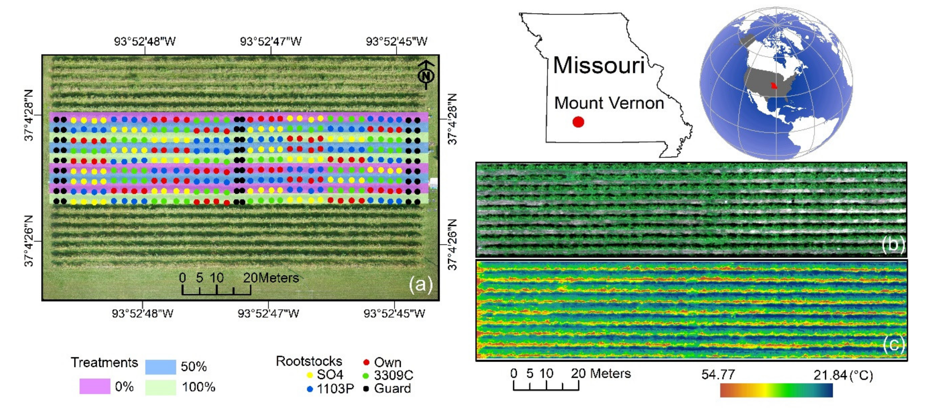
2.1. Experimental Site Description and Meteorological Measurements

Ground and aerial data were collected during the 2017 and 2018 growing seasons in a 0.9 ha experimental vineyard at the University of Missouri-Columbia Southwest Research Center in Mount Vernon, Missouri, USA (37°4′27.17″ N, 93°52′46.70″ W). The climate of the region is continental with an average annual temperature of 15.6 °C and a mean annual rainfall of 1067 mm. The experimental vineyard consists of ungrafted ‘Chambourcin’ vines and ‘Chambourcin’ scions grafted to one of the following rootstocks: Selection Oppenheim 4 (SO4), 1103 Paulsen (1103P), and 3309 Couderc (3309C). In total, the vineyard includes four scion/rootstock combinations: ‘Chambourcin ungrafted’, ‘Chambourcin/SO4’, ‘Chambourcin/1103P’, and ‘Chambourcin/3309C’. The ungrafted and grafted vines are planted in rows with 3 m row and 3 m vine spacing along the row (Figure 1a). The vineyard has an east–west row orientation. Vines were planted in 2009 and were eight years old at the beginning of sampling in this study. ‘Chambourcin’ vines were trained with a high wire cordon trellis and spur-pruned. The soil on the vineyard is a combination of sandy loam, silt loam, and loam, with an average pH of 6. Additional details of the study site are available in Maimaitiyiming et al. [64] and Maimaitiyiming et al. [65].

The ‘Chambourcin’ experimental vineyard consists of nine rows, each of which is treated with one of three different irrigation treatments, replacing 0%, 50%, and 100% of evapotranspiration (ET) losses. Each irrigation treatment is replicated three times (in three of the nine rows) and ET is obtained from a weather station installed at 270 m from the site. Each vineyard row includes 32 vines planted in cells of four adjacent vines of the same type (‘Chambourcin’ ungrafted or grafted to the same rootstocks). Within each four-vine cell, the two central vines were monitored through ground measurements.

Measurements of hourly air temperature (°C), relative humidity (%), solar radiation (Watts/m²), and wind speed (m/s) were obtained from the weather station. Vapor pressure deficit (VPD, hPa), which represents water demand of the atmosphere better than relative humidity [66], was calculated from air temperature and relative humidity using the equations of Struthers et al. [67].

2.2. Diurnal Physiological Measurements

Stomatal conductance (G_s) and steady-state chlorophyll fluorescence (F_s) were employed as important indicators of plant physiology because stomatal closure is one of the first responses to water deficit occurring in the leaves, and both G_s and F_s are closely correlated with net photosynthesis in grapevines and other species [9,68,69,70,71]. Measurements of G_s and F_s were taken at veraison (the stage at which the berries begin shifting from green to dark red, usually late July/early August) in 2018, and preharvest in 2017 and 2018 under full sun conditions, coinciding with diurnal aerial campaigns (15 September 2017, 1 August and 19 September 2018) (Figure 1).

Table 1. Summary of field campaign dates, platforms, sensors, sampling instruments, and the number of grapevines monitored for stomatal conductance (G_s) and steady-state fluorescence (F_s). On 15 September 2017, the thermal images were acquired in the midmorning (10:00 a.m.), at midday (12:45 p.m.), and in the afternoon (03:45 p.m.). On 1 August 2018, the thermal and hyperspectral images were acquired in the midmorning (11:00 a.m.), at midday (12:45 p.m.), in the midafternoon (02:00 p.m.), and afternoon (03:45 p.m.). On 19 September 2018, the thermal images were acquired in the morning (09:30 a.m.) and at midday (12:30 p.m.).

Flight Dates	Flight Time	Aerial Platforms	Sensors	Ground Sampling Distance (cm)	Growing Stages	Field Sampling Instruments	Total Number of Vines Monitored
09/15/2017	Midmorning Midday Afternoon	DJI S1000	ICI (thermal)	4	Preharvest	Fluorometer, porometer	54
08/01/2018	Midmorning Midday Midafternoon Afternoon	DJI M600	Flir (thermal), HeadWall (hyperspectral)	5 (Hyper) 9 (thermal)	Veraison	Li-6400XT	48
09/19/2018	Morning Midday	DJI S1000	ICI (thermal)	4	Preharvest	Li-6400XT	24

presents details on the field and aerial data acquisition campaigns in the two growing seasons. In 2017, G_s and F_s were measured on 2–3 sunlit, youngest fully-matured leaves (one leaf per shoot) from main exterior shoots per vine using a porometer (SC-1, Decagon, Pullman, Washington, USA) and fluorometer (FluorPen FP 110, Photon Systems Instruments, Drásov, Czech Republic), respectively. The porometer has a manufacturer-claimed measurement range of 0 to 1000 mmol H₂O m⁻² s⁻¹ with an accuracy of 10% [72]. The physiological measurements were taken from the leaves located on the upper third and sunny (south-facing) side of the canopy to represent a whole vine physiology, following previous similar studies [17,38,59]. In 2018, leaf gas exchange (G_s, photosynthetic CO₂ assimilation rate, etc.) and F_s measurements were performed on a single leaf (the same standard from the previous year was applied for leaf selection) per vine using a portable LI-6400XT infrared gas analyzer equipped with a pulse amplitude modulated leaf fluorometer chamber (Li-Cor Biosciences Inc., Lincoln, NE, USA). The leaves were measured at a controlled CO₂ concentration of 400 μmol mol⁻¹, at a photosynthetic photon flux density of 1000 μmol photons m⁻² s⁻¹, and ambient conditions of air temperature and relative humidity. Eighteen vines (four scion/rootstock combinations plus ‘Chambourcin ungrafted’ and ‘Chambourcin/SO4’ combinations for each irrigation treatment) in 2017 and twelve vines (four scion/rootstock combinations for each irrigation treatment) in 2018 were monitored for physiology at the time of each diurnal flight, representing both irrigation and rootstock treatments. This experimental design was expected to cause a wider range of vine physiological variations and afforded the ideal site for high variability in a relatively small area. Additionally, due to the time per measurement needed, it would have been unfeasible to representatively sample each subgroup to correlate with diurnal hyperspectral data.

2.3. Aerial Image Acquisition and Pre-Processing

The diurnal aerial campaigns were carried out in 2017 and 2018 using thermal and hyperspectral cameras onboard UAVs (Figure 2). Ideally, ground and aerial data collection should be carried out with the same instruments and cameras. In our case, this ideal scenario was not attainable due to limited resources and field crew availability. However, this also afforded us the opportunity to validate certain findings across multiple systems.

On 15 September 2017, a DJI S1000+ octocopter, rotary-wing platform (DJI Technology Co., Ltd., Shenzhen, China) was employed to carry an ICI (Infrared Cameras Inc.) 8640 P-Series thermal camera (Beaumont, Texas, USA) (Figure 2a,b). The aerial platform was equipped with a Pixhawk autopilot system, which enables autonomous flights based on user-defined waypoints. The ICI thermal camera was mounted on a custom-designed two-axis gimble. During the aerial campaigns, the UAV was flown at 30 m altitude above the ground with a fixed speed of 5 m/s. The ICI thermal camera has a resolution of 640 × 512 pixels in a spectral range of 7–14 μm with a 13 mm focal length, providing a ground sampling distance (GSD) of 4 cm at 30 m flight height. To successfully construct thermal orthomosaics, the flight missions were planned to have 90% forward and 80% side overlap of the thermal images, and the ICI camera was configured to capture a 14-bit radiometric JPEG image every second during the flight.

On 1 August 2018, aerial hyperspectral and thermal images were acquired using a visible and near-infrared (VNIR, 400–1000 nm) push-broom hyperspectral camera (Nano-Hyperspec VNIR model, Headwall Photonics, Fitchburg, MA, USA) installed in tandem with a FLIR (Forward-looking infrared) thermal camera (FLIR Vue Pro R 640, FLIR Systems, Inc., Wilsonville, OR, USA) onboard a DJI hexacopter (Matrice 600 Pro, DJI Technology Co., Ltd., Shenzhen, China) (Figure 2c,d). The Matrice 600 Pro is equipped with a DJI 3A Pro Flight Controller, real-time kinematic (RTK), and a Global Navigation Satellite System (GNSS) for positioning, which can provide ±0.5 m vertical and ±1.5 m horizontal accuracy. The cameras and an Applanix APX-15 global positioning system (GPS)/inertial measuring unit (IUM) (Applanix, Richmond Hill, ON, Canada) were fixed on a DJI JI Ronin-MX 3-axis gimbal, which directly connected to the aerial platform. The flight missions were carried out at an altitude of 80 m above the ground with 2 m/s forward velocity, which produced the GSDs (ground sampling distances) of 5 and 9 cm for the hyperspectral and thermal image, respectively. The hyperspectral camera records 640 spatial pixels and 270 spectral bands in the VNIR range at 2.2 nm/pixel with a radiometric resolution of 12 bits. The full width at half maximum of the camera is 6 nm with an entrance slit width of 20 μm. The hyperspectral images were acquired 40 frames per second at 2.5 ms integration time using a 12 mm focal length lens, yielding 25° of the field of view at nadir. The FLIR thermal camera has an image array of 640 × 512 pixels with a 13 mm focal length, providing 45° field of view (FOV). It can acquire longwave radiation in the 7.5–13.5 μm range at 14 bits, the thermals were recorded in a 14-bit JPEG format every second during the flights. The flight missions were planned for the hyperspectral camera with a 40% side overlap, which ensured the FLIR thermal images had at least 80% forward and side overlap because of the wide thermal camera FOV.

On 19 September 2018, thermal images were acquired using the ICI thermal camera. The flight missions and the ICI thermal camera settings were consistent with the 2017 aerial campaigns.

Both thermal cameras used in this study are radiometrically calibrated sensors, which are composed of uncooled microbolometers. Even with the radiometric calibrations provided by manufacturers, the performance of thermal cameras may be affected by atmospheric conditions, target emissivity, and distance. To improve the accuracy of derived surface temperature, these factors were accounted for by background temperature, ambient humidity, barometric pressure, target emissivity, and distance as calibration parameters and using algorithms in associated software tools. For the ICI camera, the raw thermal images were converted to surface temperature (°C) in 32-bit TIFF format by a proprietary equation within IR (Infrafred) Flash version 2.18.9.17 software (ICI, Beaumont, TX, USA), which allows adjusting atmospheric conditions and target properties. Similarly, before FLIR imaging, the temperature calibration parameters were entered to the FLIR UAS version 2.0.16 app, which can control the camera settings through Bluetooth connection from a mobile device. The calibrated thermal images were mosaiced using Pix4DMapper version 4.3.31 software (Pix4D SA, Lausanne, Switzerland) and georeferenced using the GCPs. Before each flight, the thermal cameras were turned on for at least 30 min for stabilization and the local atmospheric parameters were acquired from the on-site weather station. Additionally, a calibrated black body Model 1000 (Everest Interscience Inc., USA) and surface temperature of different objects measured with a thermal spot imager FLIR TG167 (FLIR Systems, USA, ±1.5 °C accuracy) were used for the assessment of the thermal products. For further details please see Sagan et al. [73] and Maimaitijiang et al. [74].

The hyperspectral image preprocessing included radiometric correction, orthorectification, and atmospheric correction. In the radiometric correction step, digital numbers of the raw 12-bit hyperspectral images were converted to calibrated radiometric values using the SpectralView version 5.5.1 software (Headwall Photonics, Fitchburg, MA, USA). In the same software, the calibrated radiance images were orthorectified using the Applanix IMU unit data as input. Further, the radiance was converted to reflectance in ENVI (Environment for Visualizing Images) version 5.5 software (Harris Geospatial Solutions Inc., Boulder, Colorado, USA) by the empirical line correction (ELC) method [75]. During the overpass of the aerial platform, a portable field spectroradiometer PSR-3500 (Spectral Evolution Inc., Lawrence, MA, USA) was available to provide reflectance spectra of an aerial calibration tarp with three levels of known reflectance levels (56%, 32%, and 11%), grapevines, grass, and soil, which were used as a spectral reference in the ELC method. The spectroradiometer records upwelling radiant energy in a range 350–2500 nm with a spectral resolution of 3.5 nm in the 350–1000 nm range, 10 nm in the 1000–1900 nm range, and 7 nm in the 1900–2500 nm spectral range. The targets were measured 3–5 times at nadir from 30 cm distance, and a 99% Spectralon calibration panel (Labsphere, Inc., North Sutton, NH, USA) was used to convert the target radiance to reflectance. The averaged target reflectance spectra were resampled to match the spectral resolution of the Headwall spectral camera. The radiance of the aerial images was extracted from a 25-pixel (5 by 5 pixels) region at the center of each target. Finally, the relationship between the reference spectra and the image radiance was established using the ELC method.

2.4. Extraction of Grapevine Canopy Row

To avoid the effects of shadow and soil components and due to spatial resolution discrepancy between thermal and hyperspectral images, extraction of grapevine rows is accomplished differently for thermal and hyperspectral images. Over each monitored target grapevine, a 1 m wide region of interest (width of the region was determined by canopy size) was defined and pixel values within this region were extracted for further analysis.

2.4.1. Canopy Row Extraction From Hyperspectral Images

Neural net classifiers were trained to extract pure grapevines row pixels from high-resolution hyperspectral images. We chose to use a neural net classifier due to the recent success of neural networks in hyperspectral image classification [76,77,78,79,80]. The neural net classifiers were implemented using ENVI version 5.5 software (Harris Geospatial Solutions Inc., Boulder, CO, USA) by providing regions of interest for five different classes, including grapevine, grass, vine canopy, shadow, and soil (Figure 3a). More than 6000 pixels were selected for these classes, accounting for target and illumination variability. The best performance of neural net classifiers was found using 2 hidden layers and logistic activation function with 500 training iterations. For other necessary parameters, default values were used and the parameters included training threshold contribution, training rate, training momentum, and training root mean square exit criteria. The trained neural net classifiers showed an overall accuracy better than 99.33% and a Kappa coefficient of 0.991. Figure 3b shows the results of the delineated grapevine canopy boundary.

2.4.2. Canopy Row Extraction from Thermal Images

Pure grapevine canopy pixels required for thermal image retrieval were extracted using the Canny edge detection method [81]. Canny edge detection is a multi-step algorithm that was designed to detect magnitude and orientation of image intensity changes. This method has been proven to be effective in extracting pure canopy pixels from high-resolution thermal images [82,83]. Canny edge detection was implemented using the Open-source Computer Vision library (version 4.0.0) with Python 2.7. The detected vine canopy edges were diluted by up to five pixels along the direction of the thermal gradient for more conservative extraction of the vine pixels. Finally, the vine canopy edges were converted into polyline vector and the thermal orthomosaics were clipped using the vine edge polyline vector (Figure 4).

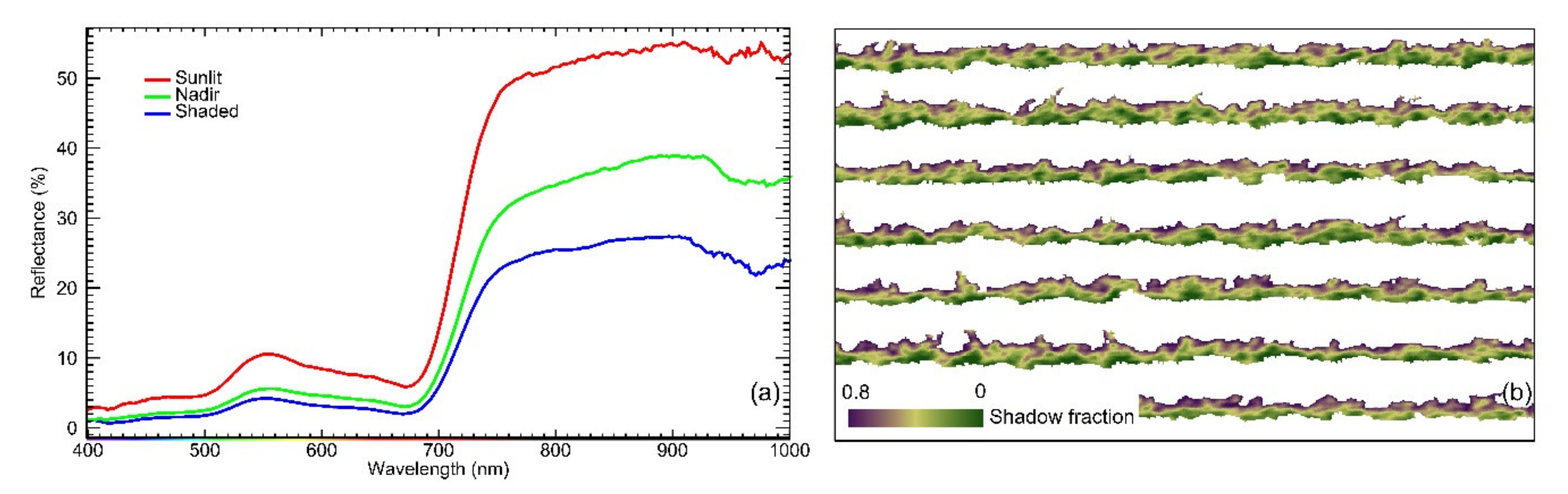
2.5. Estimation of Pixelwise Canopy Shadow Fraction

Shadowing estimates of grapevine canopy were produced using the Sequential Maximum Angle Convex Cone (SMACC) method [84]. The SMACC was developed to generate spectral endmembers and endmember abundance with less expert knowledge and time [85]. The SMACC can also calculate shadow fractions of the abundances of reflectance when the sum of the fractions of each endmember for a pixel is constrained to one or less. Shadow fraction of each grapevine canopy pixels within the hyperspectral images was estimated using the SMACC tool in ENVI software. Figure 5a and b show hyperspectral reflectance spectra of different canopy zones and canopy show fractions modeled with the SMACC method.

2.6. Grapevine Canopy Segmentation

Extracted grapevine canopies from hyperspectral and thermal images were segmented into three canopy regions, corresponding to sunlit (slt), nadir (ndr), and shaded (shd) zones using K-means clustering, a machine learning-based unsupervised clustering algorithm [86] (Figure 6 and Figure 7). K-mean clustering is an iterative algorithm that tries to find homogenous and non-overlapping clusters within data. The algorithm uses Euclidean distance as a similarity measure to minimize within-cluster variation while also keeping the clusters as different as possible. We employed K-mean clustering for vine canopy segmentation, where we grouped canopy pixels with similar shadow fraction (in the case of hyperspectral images) or canopy temperature (in the case of thermal images), depending on the type of the input image. The K-means clustering was implemented to divide vine canopies into three regions (K = 3) with maximum iterations of 100 in ENVI software.

2.7. Calculation of Spectral Indices and Features from Aerial Image

2.7.1. Hyperspectral Indices and SIF Retrieval

Commonly used hyperspectral reflectance indices closely related to plant physiology, pigment concentration, structure, and water content were calculated from the hyperspectral images to assess their ability to track diurnal physiological changes.

Table 2. Hyperspectral image retrievals used in this study.

Hyperspectral Image Retrievals	Acronym	Equation	References
Xanthophyll
Photochemical reflectance index	PRI	(R570 – R531)/(R570 + R531)	[25]
Chlorophyll
Red Edge ratio index	RE	R750/R710	[90]
Structure
Normalized difference vegetation index	NDVI	(R800 – R670)/(R800 + R670)	[91]
Simple Ratio	SR	R800/R670	[92]
Water content
Water index	WI	R900/R970	[93]
Chlorophyll fluorescence
Sun-induced chlorophyll fluorescence	SIF	$(E_{out}\times L_{in}-E_{in}\times L_{ou\mathrm{t}})/\left(E_{out}-E_{in}\right)$	[87]

R stands for reflectance, and numbers are wavelengths in nanometer (nm).

summarizes specific spectral indices grouped by their categories associated with (1) xanthophyll, (2) chlorophyll, (3) structure, (4) water content, and (5) chlorophyll fluorescence. Sun-induced chlorophyll fluorescence (SIF) emission was quantified from hyperspectral radiance images using the Fraunhofer Line Depth (FLD) principle [87]. The FLD is a radiance-based in-filling method, which takes advantage of both the narrow absorption feature of O₂-A absorption and high spectral resolution [28]. Furthermore, the FLD method has shown reliable SIF retrieval performance using hyperspectral cameras with relatively broad spectral bandwidths (ranging between 5 and 7 nm FWHM), spectral sampling (lower than 2.5 nm), and signal-to-noise ratios of 300:1 or higher [22,88,89]. The FLD was calculated from a total of three bands (FLD3) in and out O₂–A feature, using Equation (1) which is described in Reference [22,36].

$$SIF=(E_{out}\times L_{in}-E_{in}\times L_{out})/\left(E_{out}-E_{in}\right)$$

(1)

where E_out is an average value of incident solar irradiance at 750 and 780 nm, L_out is an average value of target radiance at 750 nm and 780 nm, and E_in and L_in are incident solar irradiance and target radiance at 760 nm, respectively. The incident solar irradiance was measured at the time flight using the PSR spectroradiometer attached with a cosine corrector-diffuser (180°) for the entire spectral region (350–2500 nm).

2.7.2. Simplified Canopy Water Stress Index (siCWSI)

The CWSI was proposed by Jones [94] as:

$$CWSI=(T_{canopy} - T_{wet})/(T_{dry} -T_{wet}$$

(2)

where T_canopy is average canopy temperature extracted from pure vine pixels, T_wet is the temperature of fully transpiring leaves, and T_dry is temperature of non-transpiring leaves. Determination of T_wet and T_dry for conventional CWSI calculation is always climate-dependent, complex, and time-consuming [95,96,97]. Conversely, histogram analysis-based CWSI uses thermal images as a major input and it has reduced the meteorological data dependency and field measurements [82,83]. When T_wet and T_dry were obtained using a canopy temperature histogram which follows Gaussian distribution [98], it is necessary to remove mixed pixels that partially cover canopy and background, including soil, shadow, and weed [82,83]. In particular, simplified CWSI (siCWSI) developed by Bian et al. [82] was used in this study as this method outperformed other forms of CWSI in terms of monitoring plant water status from UAV-based high-resolution thermal images. To obtain siCWSI parameters, T_wet and T_dry were determined by the mean of the lowest 0.5% and the highest 0.5% of canopy temperatures, respectively. More details about the calculation of siCWSI can be found in Bian et al. [82].

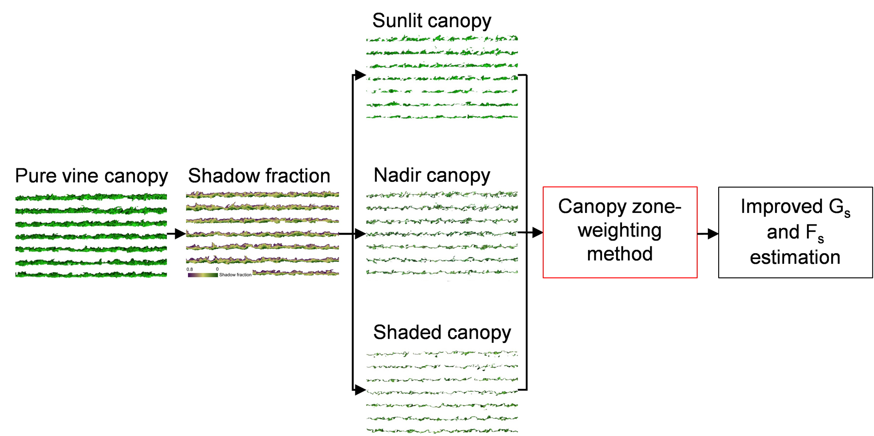
2.8. Proposed Canopy Zone-Weighting (CZW) Method

Different canopy zones are expected to bring complementary information on the targeted vine physiology measurements by mitigating effects caused by illumination, viewing angle, and canopy structure. Considering certain canopy zones show higher coefficients of determination (R²) than others in vine physiology estimation [59,61], a weighting strategy to different canopy zone can be detrimental for estimating of vine physiology. Inspired by our previous work on fusing various water quality variables and spectral reflectance through weighted prior decision-level fusion scheme [99], we herein proposed a new zone-weighting method, namely canopy zone-weighting (CZW), to systemically integrate canopy zone contribution, in which R² of each canopy zone was used to determine the contributing weight, denoted as ${\omega }_i$ in Equation (3). The integration of multiple regression model outputs may explain a wide range of variations in a target variable compared to a single regression model [100]. The proposed CZW method is expected to leverage the strengths and limit the potential biases of using a single zone-based estimation.

A summary of the implementation steps of the CZW method is described as follows: (1) Establish relationships between aerial images’ retrievals (hyperspectral indices and siCWSI) extracted from three canopy zones (slt, ndr, and shd) and grapevine physiological parameters (G_s and F_s), (2) determine the contributing weight ($\omega$) and contribution weight ratio ($c$) of the canopy zones to the target grapevine physiological indicator using the best relationships obtained in the previous step, and (3) calculate canopy zone-weighted image retrieval $(\xi$_czw) from three canopy zones using the corresponding $c$.

Relationships between the aerial image retrievals and grapevine physiological parameters were established in the form of the coefficient of determination (R²) using five different linear and non-linear regression models (e.g., second-degree polynomial, logarithmic, exponential, and power) [24], and the best R² values of the canopy zones were used to calculate the $\omega$ of each zone through Equation (3):

$${\omega }_i=\frac{1}{\frac{log{R}_i^2}{{{\displaystyle \sum }}_{i=1}^{3}log{R}_i^2}}$$

(3)

where ${\omega }_i$ is the contributing weight of $i$th canopy zone, and ${\mathrm{R}}_{\mathrm{i}}^2$ is the coefficient of determination that indicates the strength of the relationship between the $i$th canopy zone retrieval and the grapevine physiological parameters.

$c$ of the three canopy zones to the grapevine physiological parameters were calculated by:

$$c_i=\frac{{\omega }_i}{{{\displaystyle \sum }}_{i=1}^3{\omega }_i}$$

(4)

where $c_i$ is the contribution weight ratio of the $i$th canopy zone.

Based on the obtained $c$ and the original image retrievals, $\xi$_czw can be formulated by:

$${\xi }_{CZW}=c_{slt} \times {\xi }_{slt}+c_{ndr} \times {\xi }_{ndr}+c_{shd} \times {\xi }_{shd}$$

(5)

where $c_{slt}$ is the contribution weight ratio of the sunlit canopy zone, $c_{ndr}$ is the contribution weight ratio of the nadir canopy zone, and $c_{shd}$ is the contribution weight ratio of the shaded canopy zone. ${\xi }_{stl}$ is the original image retrieval of the sunlit canopy zone, ${\xi }_{ndr}$ is the original image retrieval of the nadir canopy zone, and ${\xi }_{shd}$ is the original image retrieval of the shaded canopy zone.

The aerial image retrievals derived from three canopy zones (slt, ndr, and shd), the combination of any two canopy zones (slt + ndr, slt + shd, and ndr + shd), the average value of entire canopy (avg), and the ${\xi }_{CZW}$ (CZW) were compared against G_s and F_s across all measurement time points and dates. To explore the performance of the image retrievals on the entire diurnal dataset, separate analyses were carried out for all flights together on a given field campaign date. Full relationships and their significance obtained with the linear and non-linear regression models were included as Supplementary Materials Tables S1–S3. The workflow from aerial image acquisition and preprocessing, vine canopy extraction and segmentation, and to implementation of the CWZ method and performance assessment is demonstrated in Figure 8.

3. Results

In the following sections, we report on several aspects of the experiments. First, we describe the environmental conditions of the vineyard and vine physiological indicators. Next, correlations of image retrievals (calculated from slt, ndr, shd, slt + ndr, slt + shd, ndr + shd, and avg canopy zone pixels and CZW method) with physiological indicators were analyzed to assess the effectiveness of our proposed approach. Finally, we show the diurnal changes in representative image retrievals within the vine canopy and their ability to track diurnal variations of vine physiological indicators.

3.1. Environmental Conditions and Diurnal Physiological Indicators of Grapevine

There was no major difference in the trends of environmental conditions for the three measurement dates (Figure 9). Air temperature and VPD increased gradually until 16:00 p.m., and then decreased sharply. Solar radiation followed a similar pattern as air temperature and VPD, but solar radiation rapidly rose only until midday. Relative humidity was at high levels in the morning, followed by a decreasing trend, and then began to increase from 16:00 p.m.. However, environmental conditions on 19 September 2018 were characterized by higher air temperature and lower relative humidity throughout the day compared to the previous two measurement dates, resulting in higher VPD values, thus more water-demanding atmosphere. All three measurement dates were calm, with wind speed of 3 m/s or lower, suitable for UAV data collection.

The diurnal variations of grapevine physiological indicators on all measurement dates had a similar trend. The G_s values were low in the morning, increased sharply, and reached a maximum around midday (Figure 10a,c). Afterwards, G_s decreased until the afternoon. The trend was caused, most likely, by environmental conditions. In general, the diurnal change of F_s followed the same pattern of G_s (Figure 10b,d). On most of the measurement dates, maximum F_s values occurred around noon, while lower F_s values occurred in the morning and afternoon. There were no significant differences in in-situ physiological measurements at each flight time among the irrigation and rootstock treatments. Daily G_s and F_s showed a relatively high coefficient of variation (CV). G_s had larger daily variability compared to F_s for all the measurement dates. Both G_s and F_s on 15 September 2017, had 1–2 times higher values than the values on 1 August 2018, and this could be due to the different instruments used to determine the physiological indicators. Additionally, when the same instruments were used, lower G_s and F_s values were observed on 19 September 2018 than the corresponding values on 15 September 2017. This agreed with higher VPD occurring on 19 September 2018.

3.2. Relationship between the Aerial Image Retrievals and Grapevine Physiology

On 15 September 2017, the strongest correlation was established with the midday and afternoon measurements of G_s for siCSWI_czw (R² = 0.61, p < 0.01 and R² = 0.60, p < 0.01 respectively), followed by siCWSI_avg in the midmorning (R² = 0.30, p < 0.05) (Figure 11a). siCSWI_czw provided the strongest relationship to F_s in the midmorning and midday (R² = 0.82, p < 0.001 and R² = 0.83, p < 0.001, respectively), followed by siCWSI_ndr in the afternoon (R² = 0.52, p < 0.01) (Figure 11b). Comparing the correlations from pooled three flights, both G_s and F_s were strongly correlated with siCWSI_czw (R² = 0.71, p < 0.01 and R² = 0.73, p < 0.01), followed by siCWSI_avg with G_s and siCWSI_slt+ndr with F_s, respectively.

On 1 August 2018, PRI, SIF, and siCWSI captured diurnal changes in G_s and F_s as a function of grapevine physiological response. There were no noticeable canopy structural effects, pigments degradation, and canopy water content change between irrigation treatments during the hyperspectral imaging campaign. This resulted in weak correlations (R² ≤ 0.30) between RE, NDVI, SR, and WI and grapevine physiological parameters (G_s and F_s). Similar results were observed for both separate flights and when all flights were combined. Therefore, the results and discussion sections were focused on the results of PRI and SIF for hyperspectral data analysis.

PRI more strongly correlated with G_s during afternoon hours (2:00 p.m. and 3:45 p.m.) than earlier hours (11:00 a.m. and 12:45 p.m.), while SIF showed a strong correlation with G_s for all four flights (Figure 12a,b). When three canopy zones were considered separately, PRI_slt and PRI_ndr seemed to be correlated well with G_s. For SIF, there was no single canopy zone that showed a consistently strong relationship with G_s (R² ≤ 0.60). In most cases, PRI and SIF derived from two combined canopy zones had a slightly higher correlation with G_s than that of a single canopy zone. Meanwhile, slightly lower relationships were found by comparing PRI_avg, and SIF_avg and G_s, except for the PRI_avg in the afternoon, where PRI_avg showed the highest correlation (R² = 0.96, p < 0.001) compared to any PRI from single canopy zone or combination of two. Generally, PRI_czw and SIF_czw improved the relationship with G_s. In particular, PRI_czw showed the strongest correlation in the midmorning and afternoon (R² = 0.35, p < 0.01 and R² = 0.98 p < 0.001). On the other hand, SIF_czw appeared to have the closest relationship with G_s in the midmorning (R² = 0.45, p < 0.05). When all flights were analyzed together, the relationships between PRI_czw and SIF_czw were stronger than the relationship with PRI and SIF derived from any single, combined, and average canopy zone pixels (R² = 0.70, p < 0.01 and R² = 0.89, p < 0.001).

Regarding F_s, the obtained results for all the flights showed trends similar to those found for G_s (Figure 12c,d). Both PRI and SIF showed a strong and significant relationship with F_s. PRI_sunlit (midmorning and midday) and PRI_slt+ndr (midafternoon and afternoon) showed the best fitting with F_s, while SIF_czw was well-correlated with F_s for all the flights, except for midmorning. When four flights combined, the best correlations were obtained with PRI_czw and SIF_czw, yielding (R² = 0.76, p < 0.001 and R² = 0.89, p < 0.001).

The highest correlation emerged between siCSWI_czw and G_s in the midmorning and afternoon (R² = 0.98, p < 0.001 and R² = 0.47, p < 0.01) (Figure 12e). However, in the midday and midafternoon, siCWSI_slt+shd and siCWSI_ndr respectively, showed the strongest relationship with G_s (R² = 0.89, p < 0.001 and R² = 0.96, p < 0.001), followed by siCWSI_czw at both time points (R² = 0.87, p < 0.001 and R² = 0.91, p < 0.001). The strength of the relationship for siCWSI_ndr was the strongest with F_s in the midafternoon (R² = 0.96, p < 0.001), followed by sCSWI_czw (R² = 0.95, p < 0.001) (Figure 12f). The strongest correlation was observed between siCWSI_slt+shd and F_s midmorning and afternoon, respectively (R² = 0.80, p < 0.01 and R² = 0.88, p < 0.001). siCWSI_czw was strongly correlated to F_s only in the midday (R² = 0.72, p < 0.01). Using all four diurnal datasets, the strongest correlation was found between siCWSI_czw and both G_s and F_s (R² = 0.75, p < 0.01 and R² = 0.74, p < 0.01).

On 19 September 2018, siCWSI_czw showed the strongest relationship with G_s in the morning and for the combined datasets of two flights carried out on this date (R² = 0.70, p < 0.01 and R² = 0.60, p < 0.01) (Figure 13a). During the midday, the highest correlation was found between siCWSI_ndr+shd and G_s (R² = 0.59, p < 0.01). For F_s, siCWSI_ndr+shd and siCWSI_slt+ndr had the best correlation with F_s in the morning and midday (R² = 0.59, p < 0.01 and R² = 0.73, p < 0.001) respectively, which were followed by siCWSI_czw at both time points (R² = 0.56, p < 0.01 and R² = 0.70, p < 0.01) (Figure 13b). When datasets from two flights were combined, siCWSI_czw was the most highly correlated with F_s (R² = 0.71, p < 0.01).

3.3. Diurnal Changes in Aerial Image Retrievals and Tracking Physiological Indicators

SIF and siCWSI retrievals from the VHR images on 1 August 2018 showed diurnal changes in the vine canopy (Figure 14 and Figure 15). It can be noted that there was no visual difference between irrigation and rootstock treatments, and this was consistent with the in-situ physiological measurements. However, visual differences between sunlit, nadir, and shaded canopy zones could be easily recognized in both SIF and siCWSI images. Within-canopy variability of SIF increased until midday and then decreased (Figure 14b–e), following the gradual decline in solar radiation. The highest within-canopy variability of siCWSI was observed in the afternoon (Figure 15d), when air temperature and VPD reached the maximum values for the day. In general, the effects of diurnally changing environmental factors such as solar radiation, air temperature, and VPD on the vine canopies corroborate the need to separate canopy zones, as is shown with SIF and siCWSI retrievals. Furthermore, wide ranges of SIF and siCWSI values were found (1–6.5 W sr⁻¹ m⁻² nm⁻¹ and 0.1–1, respectively) for each flight, which confirmed the relevance of canopy heterogeneity and the pertinence of accounting for the variability related to canopy structure.

The in-situ physiological indicators measured on 1 August 2018 were compared against PRI, SIF, and siCWSI to assess the diurnal trends (Figure 16). Diurnal PRI, SIF, and siCWSI values for each measurement time point showed agreements with G_s and F_s (regardless of the opposite direction shown in Figure 16a,c). Generally, these figures showed that diurnal PRI, SIF, and siCWSI followed the same pattern as that followed by vine physiological indicators during the experiment.

4. Discussion

Using diurnal VHR aerial images and in-situ physiological measurements, the current study investigated relationships between aerial image retrievals from different canopy zones and grapevine physiological indicators. Implemented irrigation treatments and rootstock/scion combinations in this study provided a wide range of grapevine physiological status for testing the capability of aerial images in characterizing grapevine physiology. The pure grapevine canopy pixels were extracted with high confidence from the high spatial resolution images coupled with neural network and computer vision-based methods. Then, the vine canopy was segmented into three different canopy zones using an unsupervised machine learning algorithm. Additionally, the siCWSI values were well within the range of the theoretical CWSI limit (<1), confirming that calculated siCWSI was based on pure vegetation pixels and not subjected to soil background contamination. It is worth mentioning that the employed methods in this study stood out among the limited similar studies [17,38,59] by taking full advantage of spectral information and temperature data as the basis for identifying different canopy zones and applying automated methods to streamline canopy zone segmentation from hyperspectral and thermal images.

4.1. Contribution of Different Canopy Zones to Grapevine Physiology: Hyperspectral Image Retrievals

In line with previous studies [22,101,102,103], PRI and SIF derived from high-resolution aerial images closely followed the diurnal physiological changes of grapevine indicated by G_s and F_s (Figure 16). The results of sunlit, nadir, and shaded canopy zones showed different levels of correlation with grapevine physiology depending on the type of aerial images and retrievals. There were only a few instances where a single canopy zone (either sunlit or nadir) showed the strongest correlations. PRI and SIF derived from either combination of two canopy zones (slt + shd more frequent than slt + ndr) or averaged entire canopy zone pixels showed the most frequent and the strongest correlation with G_s and F_s measurements.

Among the recent efforts to improve the ability of PRI, some studies indicated the strong dependence of PRI on canopy shadow fraction and confirmed the importance of shaded leaves in the simulation of canopy PRI [104,105]. Zhang et al. [106] used a two-leaf (sunlit and shaded leaves) approach to improve the ability of PRI as a proxy of light use efficacy, which is closely related to G_s, by accounting for sunlit and shaded leaf portion with weighted leaf area index. Takala and Mõttus [84] explained the illumination-related apparent variation in canopy PRI by considering shadow effects. The results of this study confirmed the importance of considering both sunlit and shaded canopy zones to improve the ability of PRI in tracking diurnal physiological changes.

SIF is also influenced by illumination, sunlit/shaded canopy, and soil background, and these influences intensify when very-high-resolution hyperspectral images are used for analysis [17,36]. Hernández et al. [17] and Camino et al [38], who considered the effects of canopy heterogeneity on SIF, demonstrated the significance of sunlit canopy pixels in determining tree physiological status and underperformance of entire canopy pixels. This is somewhat contradictory to what was observed in this study, where SIF from entire canopy pixels also performed well in multiple instances, and this could be attributed to the discrepancy in spatial resolution of the hyperspectral images used in this study (5 cm) and previous studies (20 and 60 cm, respectively), where canopy pixels tend to be easily contaminated by soil and shaded background. In general, our results showed the improvements from combined (slt + ndr and slt + shd) or entire canopy zones over sunlit zones, implying the importance of heterogeneity within canopy structure in determining the relationship between SIF and in-situ physiological measurements.

4.2. Contribution of Different Canopy Zones to Grapevine Physiology: Thermal Image Retrieval

The results from this study regarding the relationship between the siCWSI and the physiological indicators were in agreement with those from previous reports [103,107]. Canopy temperature is affected by tree structure, which in turn affects thermal image indices such as CWSI [31,32]. Furthermore, there is a lack of consensus regarding the section of the sampling zones (sunlit, nadir, and shaded zones). Sepúlveda et al. [59] and Belfiore [108] suggested to take into consideration the effect of selecting canopy zones to analyze thermal images. Suárez et al. [33] and Sepulcre et al. [107] found a stronger relationship between canopy temperature and plant physiology in the morning than midday hours and indicated the importance of high spatial resolution thermal images to minimize the intensified midday soil effects. This was not the case in this study as siCWSI consistently showed strong diurnal correlation with in-situ measurements, suggesting that midday soil thermal effects may have been avoided with pure canopy pixel extracted from high-resolution thermal images using the computer-vision-based method. However, the results showed the slightly weaker relationship between siCWSI and physiological indicators at preharvest (15 September 2017 and 19 September 2018) than veraison (1 August 2018), while thermal images collected at veraison had a lower spatial resolution. This finding may be attributable to the different growing stage because later in the season, grapevines are more likely to be senescent [109] and in-situ measurements may not represent the physiology of the whole canopy well [59,63].

4.3. Canopy Zone-Weighting (CZW) Method Provided the Most Robust Estimates of Correlations between Aerial Image Retrievals and Grapevine Physiology

Traditionally, image retrievals were calculated over canopy pixels and averaged for each sampling location for in-situ measurements. With recent advancements in UAV and sensor technology, high spatial resolution aerial images have made it possible to identify pure canopy pixels, and sunlit and shaded portions within tree canopies [17,38,56]. When it comes to high-resolution hyperspectral imagery, Hernández-Clemente et al. and Camino et al. [17,38] suggested separating sunlit and shaded canopy zones to minimize the effects of within-canopy shadows caused by the illumination condition and canopy heterogeneity. Similarly, Sepúlveda-Reyes et al. and Pou et al. [59,61] divided vine canopy into sunlit, nadir, and shaded zones in thermal imagery and found conflicting results in terms of selecting an effective canopy zone as a proxy for physiology. The CZW method proposed in this study utilized the accumulated contribution of different canopy zones within the tree canopy instead of using a mean value averaged over a certain portion of the canopy or entire canopy. Compared to conventional ways of calculating image retrievals (using only sunlit pixels, while ignoring the shaded pixels), the CZW better characterized the grapevine canopy heterogeneity, and thus grapevine physiology. Generally, our study is the only case that revealed the complementary relationships between different canopy zones using the CZW method for tracking diurnal physiological changes.

The performance of different image retrieval from different canopy zones was evaluated for each field measurement time point and all the measurement time points together for the given field date. The availability of thermal images enabled us to investigate the robustness of the CZW method over multiple growing seasons (2017 and 2018) and stages (veraison and preharvest). When a single measurement point was considered, our results showed that PRI_czw, SIF_czw, and siCWSI_czw were better related to G_s and F_s in some cases than the image retrieval from a single canopy zone, the combination of any two canopy zones, and the entire canopy. When all flights were analyzed, CZW-based retrievals always performed better than any other retrieval approaches, suggesting that CZW indeed worked well regardless of hyperspectral or thermal images when there were large variations both in image data and field measurements determined by illumination, bidirectional reflectance factor (BRDF), within-canopy heterogeneity, and diurnal physiological changes. It is worth noting here that the CWZ would have led to even better performance if the irrigation treatments had induced strong physiological changes during the flights (that was not the case here).

It is commonly accepted that recorded radiance and temperature from vegetation canopies are subject to effects of sun angle, BRDF (especially in the case of hyperspectral imaging), shadows, canopy background, structure, and leaf angle distribution, which in turn contribute to the changes in the results to a different degree. This is also true even though the aerial images used in this study were acquired at low altitudes on sunny days with stable atmospheric conditions. Additionally, these effects may vary depending on the different canopy zones used in this study. Therefore, it would be a logical follow-up effort to carry out a full analysis of the sensitivity of the relationship between image retrievals and plant physiology, focusing on normalization or mitigation of these effects specifically for each canopy zone.

4.4. Outlook

While the proposed CZW method has been demonstrated to be a promising advancement, further improvements may include the application of a pixel-weighting approach and data fusion. Indeed, leaf photosynthetic status, water content, pigment concentration, leaf angle distribution, and canopy architecture were spatially different within each canopy zone that was considered in this study. Some of these spatial changes can be explained through rich spectral information within a pixel from hyperspectral images, and thus provide important information about the plant physiology. LiDAR (Light Detection and Ranging) or photogrammetric point clouds, on the other hand, allow us to obtain accurate information about the canopy architecture and the heterogeneity within the canopy. Weighted pixels containing spectral, thermal, and structural information can be combined and will contribute to an improved understanding of plant physiology. Note that the integration of multisensory image data requires a highly accurate co-registration. Despite the relatively diverse dataset (i.e., diurnal, two growing seasons and stages for thermal images, and a single growing season and stage for hyperspectral image), further work is needed to explore the robustness of the CZW method on different growing stages of grapevines, presence of a wide range of structural and pigment changes, and tree species other than grapevines.

5. Conclusions

This study aimed to maximize the benefits of VHR hyperspectral and thermal UAV images to improve the relationship between the aerial image retrievals and diurnal indicators of grapevine physiology. Ultimately, this work allowed us to characterize physiological parameters at a scale and with speed not possible through other traditional measurements of vine physiology. Besides enabling extraction of grapevine canopy with high confidence from both hyperspectral and thermal images, the VHR images made it feasible to quantitatively analyze the contribution of different canopy zones for characterizing diurnal physiological indicators. We proposed the CZW method and evaluated its performance against the traditional image retrieval methods. The results indicated that PRI, SIF, and siCWSI from sunlit and nadir zones provided the best estimate of G_s and F_s when a single canopy zone was considered. At a single flight, PRI, SIF, and siCWSI computed over the combination of two canopy zones (sunlit + nadir, sunlit + shaded, or nadir + shaded) or entire canopy pixels showed a better relationship with diurnal G_s and F_s changes than the PRI, SIF, and siCWSI calculated over a single canopy zone. Importantly, the most frequent and the highest correlations were found for G_s and F_s with PRI_czw, SIF_czw, and siCWSI_czw. When all flights combined for the given field campaign date, PRI_czw, SIF_czw, and siCWSI_czw always significantly improved the relationship with G_s and F_s. In summary, this study first introduced the CZW concept to VHR hyperspectral and thermal UAV imageries and provided a new train of thought to the research and application of VHR images for remote assessment of plant physiological indicators.

References

1. Vivier, M.A.; Pretorius, I.S. Genetically tailored grapevines for the wine industry. Trends Biotechnol. 2002, 20, 472–478. [Google Scholar] [CrossRef]
2. Intrigliolo, D.S.; Castel, J.R. Interactive effects of deficit irrigation and shoot and cluster thinning on grapevine cv. Tempranillo. Water relations, vine performance and berry and wine composition. Irrig. Sci. 2011, 29, 443–454. [Google Scholar] [CrossRef]
3. Intrigliolo, D.S.; Pérez, D.; Risco, D.; Yeves, A.; Castel, J.R. Yield components and grape composition responses to seasonal water deficits in Tempranillo grapevines. Irrig. Sci. 2012, 30, 339–349. [Google Scholar] [CrossRef]
4. Mirás-Avalos, J.M.; Buesa, I.; Llacer, E.; Jiménez-Bello, M.A.; Risco, D.; Castel, J.R.; Intrigliolo, D.S. Water versus source–sink relationships in a semiarid Tempranillo vineyard: Vine performance and fruit composition. Am. J. Enol. Vitic. 2017, 68, 11–22. [Google Scholar] [CrossRef]
5. Chaves, M.M.; Zarrouk, O.; Francisco, R.; Costa, J.M.; Santos, T.; Regalado, A.P.; Rodrigues, M.L.; Lopes, C.M. Grapevine under deficit irrigation: Hints from physiological and molecular data. Ann. Bot. 2010, 105, 661–676. [Google Scholar] [CrossRef] [Green Version]
6. Chaves, M.M.; Santos, T.P.; Souza, C.D.; Ortuño, M.; Rodrigues, M.; Lopes, C.; Maroco, J.; Pereira, J.S. Deficit irrigation in grapevine improves water-use efficiency while controlling vigour and production quality. Ann. Appl. Biol. 2007, 150, 237–252. [Google Scholar] [CrossRef]
7. Reynolds, A.G.; Wardle, D.A.; Naylor, A.P. Impact of training system, vine spacing, and basal leaf removal on Riesling. Vine performance, berry composition, canopy microclimate, and vineyard labor requirements. Am. J. Enol. Vitic. 1996, 47, 63–76. [Google Scholar]
8. Ferrandino, A.; Lovisolo, C. Abiotic stress effects on grapevine (Vitis vinifera L.): Focus on abscisic acid-mediated consequences on secondary metabolism and berry quality. Environ. Exp. Bot. 2014, 103, 138–147. [Google Scholar] [CrossRef]
9. Cifre, J.; Bota, J.; Escalona, J.M.; Medrano, H.; Flexas, J. Physiological tools for irrigation scheduling in grapevine (Vitis vinifera L.): An open gate to improve water-use efficiency? Agric. Ecosyst. Environ. 2005, 106, 159–170. [Google Scholar] [CrossRef]
10. Hall, A.; Lamb, D.; Holzapfel, B.; Louis, J. Optical remote sensing applications in viticulture—A review. Aust. J. Grape Wine Res. 2002, 8, 36–47. [Google Scholar] [CrossRef]
11. Rapaport, T.; Hochberg, U.; Shoshany, M.; Karnieli, A.; Rachmilevitch, S. Combining leaf physiology, hyperspectral imaging and partial least squares-regression (PLS-R) for grapevine water status assessment. ISPRS J. Photogramm. Remote Sens. 2015, 109, 88–97. [Google Scholar] [CrossRef]
12. Trought, M.C.; Bramley, R.G. Vineyard variability in Marlborough, New Zealand: Characterising spatial and temporal changes in fruit composition and juice quality in the vineyard. Aust. J. Wine Res. 2011, 17, 79–89. [Google Scholar] [CrossRef]
13. Bramley, R. Understanding variability in winegrape production systems 2. Within vineyard variation in quality over several vintages. Aust. J. Wine Res. 2005, 11, 33–42. [Google Scholar] [CrossRef]
14. Guanter, L.; Alonso, L.; Gómez-Chova, L.; Amorós-López, J.; Vila, J.; Moreno, J. Estimation of solar-induced vegetation fluorescence from space measurements. Geophys. Res. Lett. 2007, 34. [Google Scholar] [CrossRef]
15. Sepulcre-Cantó, G.; Zarco-Tejada, P.J.; Jiménez-Muñoz, J.; Sobrino, J.; Soriano, M.; Fereres, E.; Vega, V.; Pastor, M. Monitoring yield and fruit quality parameters in open-canopy tree crops under water stress. Implications for ASTER. Remote Sens. Environ. 2007, 107, 455–470. [Google Scholar] [CrossRef]
16. Wendel, A.; Underwood, J. Illumination compensation in ground based hyperspectral imaging. ISPRS J. Photogramm. Remote Sens. 2017, 129, 162–178. [Google Scholar] [CrossRef]
17. Hernández-Clemente, R.; North, P.R.J.; Hornero, A.; Zarco-Tejada, P.J. Assessing the effects of forest health on sun-induced chlorophyll fluorescence using the FluorFLIGHT 3-D radiative transfer model to account for forest structure. Remote Sens. Environ. 2017, 193, 165–179. [Google Scholar] [CrossRef] [Green Version]
18. Aneece, I.; Thenkabail, P. Accuracies Achieved in Classifying Five Leading World Crop Types and their Growth Stages Using Optimal Earth Observing-1 Hyperion Hyperspectral Narrowbands on Google Earth Engine. Remote Sens. 2018, 10, 2027. [Google Scholar] [CrossRef] [Green Version]
19. Mariotto, I.; Thenkabail, P.S.; Huete, A.; Slonecker, E.T.; Platonov, A. Hyperspectral versus multispectral crop-productivity modeling and type discrimination for the HyspIRI mission. Remote Sens. Environ. 2013, 139, 291–305. [Google Scholar] [CrossRef]
20. Thenkabail, P.S.; Enclona, E.A.; Ashton, M.S.; Legg, C.; De Dieu, M.J. Hyperion, IKONOS, ALI, and ETM+ sensors in the study of African rainforests. Remote Sens. Environ. 2004, 90, 23–43. [Google Scholar] [CrossRef]
21. Suárez, L.; Zarco-Tejada, P.J.; Berni, J.A.; González-Dugo, V.; Fereres, E. Modelling PRI for water stress detection using radiative transfer models. Remote Sens. Environ. 2009, 113, 730–744. [Google Scholar] [CrossRef] [Green Version]
22. Zarco-Tejada, P.J.; González-Dugo, V.; Berni, J.A. Fluorescence, temperature and narrow-band indices acquired from a UAV platform for water stress detection using a micro-hyperspectral imager and a thermal camera. Remote Sens. Environ. 2012, 117, 322–337. [Google Scholar] [CrossRef]
23. Atherton, J.; Nichol, C.J.; Porcar-Castell, A. Using spectral chlorophyll fluorescence and the photochemical reflectance index to predict physiological dynamics. Remote Sens. Environ. 2016, 176, 17–30. [Google Scholar] [CrossRef]
24. Panigada, C.; Rossini, M.; Meroni, M.; Cilia, C.; Busettoa, L.; Amaducci, S.; Boschetti, M.; Cogliati, S.; Picchi, V.; Pinto, F.; et al. Fluorescence, PRI and canopy temperature for water stress detection in cereal crops. Int. J. Appl. Earth Obs. Geoinf. 2014, 30, 167–178. [Google Scholar] [CrossRef]
25. Gamon, J.; Penuelas, J.; Field, C. A narrow-waveband spectral index that tracks diurnal changes in photosynthetic efficiency. Remote Sens. Environ. 1992, 41, 35–44. [Google Scholar] [CrossRef]
26. Krause, G.H.; Weis, E. Chlorophyll fluorescence as a tool in plant physiology. Photosynth. Res. 1984, 5, 139–157. [Google Scholar] [CrossRef] [PubMed]
27. Guanter, L.; Rossini, M.; Colombo, R.; Meroni, M.; Frankenberg, C.; Lee, J.-E.; Joiner, J. Using field spectroscopy to assess the potential of statistical approaches for the retrieval of sun-induced chlorophyll fluorescence from ground and space. Remote Sens. Environ. 2013, 133, 52–61. [Google Scholar] [CrossRef]
28. Meroni, M.; Rossini, M.; Guanter, L.; Alonso, L.; Rascher, U.; Colombo, R.; Moreno, J. Remote sensing of solar-induced chlorophyll fluorescence: Review of methods and applications. Remote Sens. Environ. 2009, 113, 2037–2051. [Google Scholar] [CrossRef]
29. Moya, I.; Camenen, L.; Evain, S.; Goulas, Y.; Cerovic, Z.G.; Latouche, G.; Flexas, J.; Ounis, A. A new instrument for passive remote sensing: 1. Measurements of sunlight-induced chlorophyll fluorescence. Remote Sens. Environ. 2004, 91, 186–197. [Google Scholar] [CrossRef]
30. Inoue, Y.; Kimball, B.A.; Jackson, R.D.; Pinter, P.J.; Reginato, R.J. Remote estimation of leaf transpiration rate and stomatal resistance based on infrared thermometry. Agric. For. Meteorol. 1990, 51, 21–33. [Google Scholar] [CrossRef]
31. Idso, S.; Jackson, R.; Pinter, P., Jr.; Reginato, R.; Hatfield, J. Normalizing the stress-degree-day parameter for environmental variability. Agric. Meteorol. 1981, 24, 45–55. [Google Scholar] [CrossRef]
32. Jackson, R.D.; Idso, S.; Reginato, R.; Pinter, P. Canopy temperature as a crop water stress indicator. Water Resour. Res. 1981, 17, 1133–1138. [Google Scholar] [CrossRef]
33. Suárez, L.; Zarco-Tejada, P.J.; Sepulcre-Cantó, G.; Pérez-Priego, O.; Miller, J.R.; Jiménez-Muñoz, J.; Sobrino, J. Assessing canopy PRI for water stress detection with diurnal airborne imagery. Remote Sens. Environ. 2008, 112, 560–575. [Google Scholar] [CrossRef]
34. Rossini, M.; Fava, F.; Cogliati, S.; Meroni, M.; Marchesi, A.; Panigada, C.; Giardino, C.; Busetto, L.; Migliavacca, M.; Amaducci, S.; et al. Assessing canopy PRI from airborne imagery to map water stress in maize. ISPRS J. Photogramm. Remote Sens. 2013, 86, 168–177. [Google Scholar] [CrossRef]
35. Santesteban, L.G.; Di Gennaro, S.F.; Herrero-Langreo, A.; Miranda, C.; Royo, J.B.; Matese, A. High-resolution UAV-based thermal imaging to estimate the instantaneous and seasonal variability of plant water status within a vineyard. Agric. Water Manag. 2017, 183, 49–59. [Google Scholar] [CrossRef]
36. Zarco-Tejada, P.J.; Suárez, L.; González-Dugo, V. Spatial resolution effects on chlorophyll fluorescence retrieval in a heterogeneous canopy using hyperspectral imagery and radiative transfer simulation. IEEE Geosci. Remote Sens. 2013, 10, 937–941. [Google Scholar] [CrossRef]
37. Matese, A.; Di Gennaro, S. Practical Applications of a Multisensor UAV Platform Based on Multispectral, Thermal and RGB High Resolution Images in Precision Viticulture. Agriculture 2018, 8, 116. [Google Scholar] [CrossRef] [Green Version]
38. Camino, C.; Zarco-Tejada, P.J.; Gonzalez-Dugo, V. Effects of Heterogeneity within Tree Crowns on Airborne-Quantified SIF and the CWSI as Indicators of Water Stress in the Context of Precision Agriculture. Remote Sens. 2018, 10, 604. [Google Scholar] [CrossRef] [Green Version]
39. Chapman, S.; Merz, T.; Chan, A.; Jackway, P.; Hrabar, S.; Dreccer, M.; Holland, E.; Zheng, B.; Ling, T.; Jimenez-Berni, J. Pheno-Copter: A Low-Altitude, Autonomous Remote-Sensing Robotic Helicopter for High-Throughput Field-Based Phenotyping. Agronomy 2014, 4, 279. [Google Scholar] [CrossRef] [Green Version]
40. Gevaert, C.M.; Suomalainen, J.; Tang, J.; Kooistra, L. Generation of Spectral–Temporal Response Surfaces by Combining Multispectral Satellite and Hyperspectral UAV Imagery for Precision Agriculture Applications. IEEE J. Stars 2015, 8, 3140–3146. [Google Scholar] [CrossRef]
41. Zaman-Allah, M.; Vergara, O.; Araus, J.L.; Tarekegne, A.; Magorokosho, C.; Zarco-Tejada, P.J.; Hornero, A.; Albà, A.H.; Das, B.; Craufurd, P.; et al. Unmanned aerial platform-based multi-spectral imaging for field phenotyping of maize. Plant. Methods 2015, 11, 35. [Google Scholar] [CrossRef] [PubMed] [Green Version]
42. Araus, J.L.; Cairns, J.E. Field high-throughput phenotyping: The new crop breeding frontier. Trends Plant Sci. 2014, 19, 52–61. [Google Scholar] [CrossRef]
43. Hilker, T.; Gitelson, A.; Coops, N.C.; Hall, F.G.; Black, T.A. Tracking plant physiological properties from multi-angular tower-based remote sensing. Oecologia 2011, 165, 865–876. [Google Scholar] [CrossRef] [PubMed] [Green Version]
44. Yang, G.; Liu, J.; Zhao, C.; Li, Z.; Huang, Y.; Yu, H.; Xu, B.; Yang, X.; Zhu, D.; Zhang, X.; et al. Unmanned Aerial Vehicle Remote Sensing for Field-Based Crop Phenotyping: Current Status and Perspectives. Front. Plant Sci. 2017, 8, 1111. [Google Scholar] [CrossRef] [PubMed]
45. Gago, J.; Douthe, C.; Coopman, R.E.; Gallego, P.P.; Ribas-Carbo, M.; Flexas, J.; Escalona, J.; Medrano, H. UAVs challenge to assess water stress for sustainable agriculture. Agric. Water Manag. 2015, 153, 9–19. [Google Scholar] [CrossRef]
46. Lelong, C.; Burger, P.; Jubelin, G.; Roux, B.; Labbé, S.; Baret, F. Assessment of Unmanned Aerial Vehicles Imagery for Quantitative Monitoring of Wheat Crop in Small Plots. Sensors 2008, 8, 3557. [Google Scholar] [CrossRef] [PubMed]
47. Maes, W.H.; Steppe, K. Perspectives for Remote Sensing with Unmanned Aerial Vehicles in Precision Agriculture. Trends Plant Sci. 2018, 24, 152–164. [Google Scholar] [CrossRef] [PubMed]
48. Shi, Y.; Thomasson, J.A.; Murray, S.C.; Pugh, N.A.; Rooney, W.L.; Shafian, S.; Rajan, N.; Rouze, G.; Morgan, C.L.S.; Neely, H.L.; et al. Unmanned Aerial Vehicles for High-Throughput Phenotyping and Agronomic Research. PLoS ONE 2016, 11, e0159781. [Google Scholar] [CrossRef] [Green Version]
49. Barbedo, J.G.A. A Review on the Use of Unmanned Aerial Vehicles and Imaging Sensors for Monitoring and Assessing Plant Stresses. Drones 2019, 3, 40. [Google Scholar] [CrossRef] [Green Version]
50. Jang, G.; Kim, J.; Yu, J.-K.; Kim, H.-J.; Kim, Y.; Kim, D.-W.; Kim, K.-H.; Lee, C.W.; Chung, Y.S. Review: Cost-Effective Unmanned Aerial Vehicle (UAV) Platform for Field Plant Breeding Application. Remote Sens. 2020, 12, 998. [Google Scholar] [CrossRef] [Green Version]
51. Sankaran, S.; Khot, L.R.; Espinoza, C.Z.; Jarolmasjed, S.; Sathuvalli, V.R.; Vandemark, G.J.; Miklas, P.N.; Carter, A.H.; Pumphrey, M.O.; Knowles, N.R. Low-altitude, high-resolution aerial imaging systems for row and field crop phenotyping: A review. Eur. J. Agron. 2015, 70, 112–123. [Google Scholar] [CrossRef]
52. Guan, S.; Fukami, K.; Matsunaka, H.; Okami, M.; Tanaka, R.; Nakano, H.; Sakai, T.; Nakano, K.; Ohdan, H.; Takahashi, K. Assessing Correlation of High-Resolution NDVI with Fertilizer Application Level and Yield of Rice and Wheat Crops Using Small UAVs. Remote Sens. 2019, 11, 112. [Google Scholar] [CrossRef] [Green Version]
53. Yeom, J.; Jung, J.; Chang, A.; Maeda, M.; Landivar, J. Automated Open Cotton Boll Detection for Yield Estimation Using Unmanned Aircraft Vehicle (UAV) Data. Remote Sens. 2018, 10, 1895. [Google Scholar] [CrossRef] [Green Version]
54. Rasmussen, J.; Nielsen, J.; Garcia-Ruiz, F.; Christensen, S.; Streibig, J.C. Potential uses of small unmanned aircraft systems (UAS) in weed research. Weed Res. 2013, 53, 242–248. [Google Scholar] [CrossRef]
55. Gao, J.; Liao, W.; Nuyttens, D.; Lootens, P.; Vangeyte, J.; Pižurica, A.; He, Y.; Pieters, J.G. Fusion of pixel and object-based features for weed mapping using unmanned aerial vehicle imagery. Int. J. Appl. Earth Obs. Geoinf. 2018, 67, 43–53. [Google Scholar] [CrossRef]
56. Jay, S.; Baret, F.; Dutartre, D.; Malatesta, G.; Héno, S.; Comar, A.; Weiss, M.; Maupas, F. Exploiting the centimeter resolution of UAV multispectral imagery to improve remote-sensing estimates of canopy structure and biochemistry in sugar beet crops. Remote Sens. Environ. 2019, 231, 110898. [Google Scholar] [CrossRef]
57. Zarco-Tejada, P.J.; Guillén-Climent, M.L.; Hernández-Clemente, R.; Catalina, A.; González, M.R.; Martín, P. Estimating leaf carotenoid content in vineyards using high resolution hyperspectral imagery acquired from an unmanned aerial vehicle (UAV). Agric. Forest Meteorol. 2013, 171–172, 281–294. [Google Scholar] [CrossRef] [Green Version]
58. Berni, J.A.J.; Zarco-Tejada, P.J.; Sepulcre-Cantó, G.; Fereres, E.; Villalobos, F. Mapping canopy conductance and CWSI in olive orchards using high resolution thermal remote sensing imagery. Remote Sens. Environ. 2009, 113, 2380–2388. [Google Scholar] [CrossRef]
59. Sepúlveda-Reyes, D.; Ingram, B.; Bardeen, M.; Zúñiga, M.; Ortega-Farías, S.; Poblete-Echeverría, C. Selecting canopy zones and thresholding approaches to assess grapevine water status by using aerial and ground-based thermal imaging. Remote Sens. 2016, 8, 822. [Google Scholar] [CrossRef] [Green Version]
60. Reinert, S.; Bögelein, R.; Thomas, F.M. Use of thermal imaging to determine leaf conductance along a canopy gradient in European beech (Fagus sylvatica). Tree Physiol. 2012, 32, 294–302. [Google Scholar] [CrossRef] [Green Version]
61. Pou, A.; Diago, M.P.; Medrano, H.; Baluja, J.; Tardaguila, J. Validation of thermal indices for water status identification in grapevine. Agric. Water Manag. 2014, 134, 60–72. [Google Scholar] [CrossRef]
62. Baluja, J.; Diago, M.P.; Balda, P.; Zorer, R.; Meggio, F.; Morales, F.; Tardaguila, J. Assessment of vineyard water status variability by thermal and multispectral imagery using an unmanned aerial vehicle (UAV). Irrig. Sci. 2012, 30, 511–522. [Google Scholar] [CrossRef]
63. Möller, M.; Alchanatis, V.; Cohen, Y.; Meron, M.; Tsipris, J.; Naor, A.; Ostrovsky, V.; Sprintsin, M.; Cohen, S. Use of thermal and visible imagery for estimating crop water status of irrigated grapevine. J. Exp. Bot. 2006, 58, 827–838. [Google Scholar] [CrossRef] [PubMed] [Green Version]
64. Maimaitiyiming, M.; Ghulam, A.; Bozzolo, A.; Wilkins, J.L.; Kwasniewski, M.T. Early Detection of Plant Physiological Responses to Different Levels of Water Stress Using Reflectance Spectroscopy. Remote Sens. 2017, 9, 745. [Google Scholar] [CrossRef] [Green Version]
65. Maimaitiyiming, M.; Sagan, V.; Sidike, P.; Kwasniewski, M.T. Dual Activation Function-Based Extreme Learning Machine (ELM) for Estimating Grapevine Berry Yield and Quality. Remote Sens. 2019, 11, 740. [Google Scholar] [CrossRef] [Green Version]
66. Anderson, D.B. Relative humidity or vapor pressure deficit. Ecology 1936, 17, 277–282. [Google Scholar] [CrossRef]
67. Struthers, R.; Ivanova, A.; Tits, L.; Swennen, R.; Coppin, P. Thermal infrared imaging of the temporal variability in stomatal conductance for fruit trees. Int. J. App. Earth Obs. Geoinf. 2015, 39, 9–17. [Google Scholar] [CrossRef]
68. Flexas, J.; Briantais, J.-M.; Cerovic, Z.; Medrano, H.; Moya, I. Steady-State and Maximum Chlorophyll Fluorescence Responses to Water Stress in Grapevine Leaves: A New Remote Sensing System. Remote Sens. Environ. 2000, 73, 283–297. [Google Scholar] [CrossRef]
69. Papageorgiou, G.C. Chlorophyll a Fluorescence: A Signature of Photosynthesis; Springer Science & Business Media: Berlin/Heidelberg, Germany, 2007; Volume 19. [Google Scholar]
70. Zarco-Tejada, P.J.; Catalina, A.; González, M.; Martín, P. Relationships between net photosynthesis and steady-state chlorophyll fluorescence retrieved from airborne hyperspectral imagery. Remote Sens. Environ. 2013, 136, 247–258. [Google Scholar] [CrossRef] [Green Version]
71. Rahmati, M.; Mirás-Avalos, J.M.; Valsesia, P.; Lescourret, F.; Génard, M.; Davarynejad, G.H.; Bannayan, M.; Azizi, M.; Vercambre, G. Disentangling the effects of water stress on carbon acquisition, vegetative growth, and fruit quality of peach trees by means of the QualiTree model. Front. Plant Sci. 2018, 9, 3. [Google Scholar] [CrossRef] [Green Version]
72. Decagon Devices. Leaf Porometer—Operator’s Manual: Version: October 17, 2016; Decagon Devices: Pullman, WA, USA, 2016. [Google Scholar]
73. Sagan, V.; Maimaitijiang, M.; Sidike, P.; Eblimit, K.; Peterson, K.T.; Hartling, S.; Esposito, F.; Khanal, K.; Newcomb, M.; Pauli, D.; et al. UAV-Based High Resolution Thermal Imaging for Vegetation Monitoring, and Plant Phenotyping Using ICI 8640 P, FLIR Vue Pro R 640, and thermoMap Cameras. Remote Sens. 2019, 11, 330. [Google Scholar] [CrossRef] [Green Version]
74. Maimaitijiang, M.; Sagan, V.; Sidike, P.; Hartling, S.; Esposito, F.; Fritschi, F.B. Soybean yield prediction from UAV using multimodal data fusion and deep learning. Remote Sens. Environ. 2020, 237, 111599. [Google Scholar] [CrossRef]
75. Conel, J.E.; Green, R.O.; Vane, G.; Bruegge, C.J.; Alley, R.E.; Curtiss, B.J. AIS-2 radiometry and a comparison of methods for the recovery of ground reflectance. In Proceedings of the Third Airborne Imaging Spectrometer Data Analysis Workshop, Pasadena, CA, USA, 8–10 April 1985. [Google Scholar]
76. Raczko, E.; Zagajewski, B. Comparison of support vector machine, random forest and neural network classifiers for tree species classification on airborne hyperspectral APEX images. Eur. J. Remote Sens. 2017, 50, 144–154. [Google Scholar] [CrossRef] [Green Version]
77. Nevalainen, O.; Honkavaara, E.; Tuominen, S.; Viljanen, N.; Hakala, T.; Yu, X.; Hyyppä, J.; Saari, H.; Pölönen, I.; Imai, N. Individual tree detection and classification with UAV-based photogrammetric point clouds and hyperspectral imaging. Remote Sens. 2017, 9, 185. [Google Scholar] [CrossRef] [Green Version]
78. Sidike, P.; Sagan, V.; Maimaitijiang, M.; Maimaitiyiming, M.; Shakoor, N.; Burken, J.; Mockler, T.; Fritschi, F.B. dPEN: Deep Progressively Expanded Network for mapping heterogeneous agricultural landscape using WorldView-3 satellite imagery. Remote Sens. Environ. 2019, 221, 756–772. [Google Scholar] [CrossRef]
79. Essa, A.; Sidike, P.; Asari, V. Volumetric Directional Pattern for Spatial Feature Extraction in Hyperspectral Imagery. IEEE Geosci. Remote Sens. 2017, 14, 1056–1060. [Google Scholar] [CrossRef]
80. Sumsion, G.R.; Bradshaw, M.S.; Hill, K.T.; Pinto, L.D.G.; Piccolo, S.R. Remote sensing tree classification with a multilayer perceptron. PeerJ 2019, 7, e6101. [Google Scholar] [CrossRef] [Green Version]
81. Canny, J. A computational approach to edge detection. IEEE Trans. Pattern Anal. Mach. Intell. 1986, 679–698. [Google Scholar] [CrossRef]
82. Bian, J.; Zhang, Z.; Chen, J.; Chen, H.; Cui, C.; Li, X.; Chen, S.; Fu, Q. Simplified Evaluation of Cotton Water Stress Using High Resolution Unmanned Aerial Vehicle Thermal Imagery. Remote Sens. 2019, 11, 267. [Google Scholar] [CrossRef] [Green Version]
83. Park, S.; Ryu, D.; Fuentes, S.; Chung, H.; Hernández-Montes, E.; O’Connell, M. Adaptive Estimation of Crop Water Stress in Nectarine and Peach Orchards Using High-Resolution Imagery from an Unmanned Aerial Vehicle (UAV). Remote Sens. 2017, 9, 828. [Google Scholar] [CrossRef] [Green Version]
84. Takala, T.L.H.; Mõttus, M. Spatial variation of canopy PRI with shadow fraction caused by leaf-level irradiation conditions. Remote Sens. Environ. 2016, 182, 99–112. [Google Scholar] [CrossRef]
85. Gruninger, J.H.; Ratkowski, A.J.; Hoke, M.L. The sequential maximum angle convex cone (SMACC) endmember model. In Algorithms and Technologies for Multispectral, Hyperspectral, and Ultraspectral Imagery X, Proceedings of SPIE; Orlando, FL, USA, 12–15 April 2004, Shen, S.S., Lewis, P.E., Eds.; SPIE: Bellingham, WA, USA, 2004; Volume 5425, pp. 1–14. [Google Scholar]
86. MacQueen, J. Some methods for classification and analysis of multivariate observations. In Proceedings of the Fifth Berkeley Symposium on Mathematical Statistics and Probability, Berkeley, CA, USA, 21 June–18 July 1967; Volume 1, pp. 281–297. [Google Scholar]
87. Plascyk, J.A.; Gabriel, F.C. The Fraunhofer line discriminator MKII-an airborne instrument for precise and standardized ecological luminescence measurement. IEEE Trans. Instrum. Meas. 1975, 24, 306–313. [Google Scholar] [CrossRef]
88. Camino, C.; Gonzalez-Dugo, V.; Hernandez, P.; Zarco-Tejada, P.J. Radiative transfer Vcmax estimation from hyperspectral imagery and SIF retrievals to assess photosynthetic performance in rainfed and irrigated plant phenotyping trials. Remote Sens. Environ. 2019, 111186. [Google Scholar] [CrossRef]
89. Damm, A.; Erler, A.; Hillen, W.; Meroni, M.; Schaepman, M.E.; Verhoef, W.; Rascher, U. Modeling the impact of spectral sensor configurations on the FLD retrieval accuracy of sun-induced chlorophyll fluorescence. Remote Sens. Environ. 2011, 115, 1882–1892. [Google Scholar] [CrossRef]
90. Zarco-Tejada, P.J.; Miller, J.R.; Noland, T.L.; Mohammed, G.H.; Sampson, P.H. Scaling-up and model inversion methods with narrowband optical indices for chlorophyll content estimation in closed forest canopies with hyperspectral data. IEEE Trans. Geosci. Remote Sens. 2001, 39, 1491–1507. [Google Scholar] [CrossRef] [Green Version]
91. Rouse, J.W., Jr.; Haas, R.; Schell, J.; Deering, D. Monitoring vegetation systems in the Great Plains with ERTS. In Proceedings of the 3rd ERTS Symposium, Washington, DC, USA, 10–14 December 1973; Volume 1, pp. 309–317. [Google Scholar]
92. Jordan, C.F. Derivation of Leaf-Area Index from Quality of Light on the Forest Floor. Ecology 1969, 50, 663–666. [Google Scholar] [CrossRef]
93. Peñuelas, J.; Filella, I.; Biel, C.; Serrano, L.; Save, R. The reflectance at the 950–970 nm region as an indicator of plant water status. Int. J. Remote Sens. 1993, 14, 1887–1905. [Google Scholar] [CrossRef]
94. Jones, H. Plants and Microclimate: A Quantitative Approach to Environmental Plant Physiology; Cambridge University Press: Cambridge, UK, 1992. [Google Scholar]
95. Alchanatis, V.; Cohen, Y.; Cohen, S.; Moller, M.; Sprinstin, M.; Meron, M.; Tsipris, J.; Saranga, Y.; Sela, E. Evaluation of different approaches for estimating and mapping crop water status in cotton with thermal imaging. Precis. Agric. 2010, 11, 27–41. [Google Scholar] [CrossRef]
96. Leinonen, I.; Jones, H.G. Combining thermal and visible imagery for estimating canopy temperature and identifying plant stress. J. Exp. Bot. 2004, 55, 1423–1431. [Google Scholar] [CrossRef] [Green Version]
97. Romero-Trigueros, C.; Bayona Gambín, J.M.; Nortes Tortosa, P.A.; Alarcón Cabañero, J.J.; Nicolás Nicolás, E. Determination of Crop Water Stress Index by Infrared Thermometry in Grapefruit Trees Irrigated with Saline Reclaimed Water Combined with Deficit Irrigation. Remote Sens. 2019, 11, 757. [Google Scholar] [CrossRef] [Green Version]
98. Meron, M.; Sprintsin, M.; Tsipris, J.; Alchanatis, V.; Cohen, Y. Foliage temperature extraction from thermal imagery for crop water stress determination. Precis. Agric. 2013, 14, 467–477. [Google Scholar] [CrossRef]
99. Peterson, K.T.; Sagan, V.; Sidike, P.; Hasenmueller, E.A.; Sloan, J.J.; Knouft, J.H.J.P.E.; Sensing, R. Machine Learning-Based Ensemble Prediction of Water-Quality Variables Using Feature-Level and Decision-Level Fusion with Proximal Remote Sensing. Photogramm. Eng. Remote Sens. 2019, 85, 269–280. [Google Scholar] [CrossRef]
100. Ghulam, A.; Kusky, T.M.; Teyip, T.; Qin, Q. Sub-canopy soil moisture modeling in n-dimensional spectral feature space. Photogramm. Eng. Remote Sens. 2011, 77, 149–156. [Google Scholar] [CrossRef]
101. Zarco-Tejada, P.J.; Berni, J.A.; Suárez, L.; Sepulcre-Cantó, G.; Morales, F.; Miller, J. Imaging chlorophyll fluorescence with an airborne narrow-band multispectral camera for vegetation stress detection. Remote Sens. Environ. 2009, 113, 1262–1275. [Google Scholar] [CrossRef]
102. Gerhards, M.; Schlerf, M.; Rascher, U.; Udelhoven, T.; Juszczak, R.; Alberti, G.; Miglietta, F.; Inoue, Y. Analysis of Airborne Optical and Thermal Imagery for Detection of Water Stress Symptoms. Remote Sens. 2018, 10, 1139. [Google Scholar] [CrossRef] [Green Version]
103. Zarco-Tejada, P.J.; González-Dugo, V.; Williams, L.E.; Suárez, L.; Berni, J.A.J.; Goldhamer, D.; Fereres, E. A PRI-based water stress index combining structural and chlorophyll effects: Assessment using diurnal narrow-band airborne imagery and the CWSI thermal index. Remote Sens. Environ. 2013, 138, 38–50. [Google Scholar] [CrossRef]
104. Hall, F.G.; Hilker, T.; Coops, N.C.; Lyapustin, A.; Huemmrich, K.F.; Middleton, E.; Margolis, H.; Drolet, G.; Black, T.A. Multi-angle remote sensing of forest light use efficiency by observing PRI variation with canopy shadow fraction. Remote Sens. Environ. 2008, 112, 3201–3211. [Google Scholar] [CrossRef] [Green Version]
105. Hilker, T.; Hall, F.G.; Coops, N.C.; Lyapustin, A.; Wang, Y.; Nesic, Z.; Grant, N.; Black, T.A.; Wulder, M.A.; Kljun, N.; et al. Remote sensing of photosynthetic light-use efficiency across two forested biomes: Spatial scaling. Remote Sens. Environ. 2010, 114, 2863–2874. [Google Scholar] [CrossRef]
106. Zhang, Q.; Chen, J.M.; Ju, W.; Wang, H.; Qiu, F.; Yang, F.; Fan, W.; Huang, Q.; Wang, Y.-P.; Feng, Y.; et al. Improving the ability of the photochemical reflectance index to track canopy light use efficiency through differentiating sunlit and shaded leaves. Remote Sens. Environ. 2017, 194, 1–15. [Google Scholar] [CrossRef]
107. Sepulcre-Cantó, G.; Zarco-Tejada, P.; Jiménez-Muñoz, J.; Sobrino, J.; de Miguel, E.; Villalobos, F. Within-field thermal variability detection as function of water stress in Olea europaea L. orchards with high spatial remote sensing imagery. Agric. For. Meteorol. 2006, 136, 31–44. [Google Scholar] [CrossRef]
108. Belfiore, N.; Vinti, R.; Lovat, L.; Chitarra, W.; Tomasi, D.; de Bei, R.; Meggio, F.; Gaiotti, F. Infrared Thermography to Estimate Vine Water Status: Optimizing Canopy Measurements and Thermal Indices for the Varieties Merlot and Moscato in Northern Italy. Agronomy 2019, 9, 821. [Google Scholar] [CrossRef] [Green Version]
109. Bellvert, J.; Marsal, J.; Girona, J.; Zarco-Tejada, P.J. Seasonal evolution of crop water stress index in grapevine varieties determined with high-resolution remote sensing thermal imagery. Irrig. Sci. 2015, 33, 81–93. [Google Scholar] [CrossRef]
Figure 1. Central irrigation treatment rows and grapevines with different rootstocks (a). Figure (b) was obtained with a Headwall Nano hyperspectral camera (red: 659.27 nm, green: 549.27 nm, and blue: 479.69 nm, true-color image). Figure (c) was obtained with an ICI (Infrared Cameras Inc.) thermal camera.
Remotesensing 12 03216 g001
Figure 2. UAV systems and interrelated sensors. DJI S1000+ UAV system (a) with ICI thermal camera (b), DJI-Matrice 600 Pro UAV system, (c) with Headwall Nano Hyperspectral and FLIR thermal cameras (d).
Remotesensing 12 03216 g002
Figure 3. Hyperspectral reflectance spectra of grapevine, grass, grapevine canopy shadow, and soil (a). The results of grapevine canopy row delineation (white outlines, b).
Remotesensing 12 03216 g003
Figure 4. The thermal images showing the extraction of pure grapevine pixels to estimate canopy temperature (red polygons). (a) Example of thermal orthomosaic acquired with ICI camera. (b) Example of thermal acquired obtained with FLIR camera.
Remotesensing 12 03216 g004
Figure 5. (a) Hyperspectral reflectance spectra of different canopy zones. (b) Canopy shadow fraction modeled with the Sequential Maximum Angle Convex Cone (SMACC) method.
Remotesensing 12 03216 g005
Figure 6. Subsets of grapevine canopy zones extracted from the hyperspectral image. (a) Entire grapevine canopy, (b) sunlit (slt) canopy zone, (c) nadir (ndr) canopy zone, (d) shaded (shd) canopy zone.
Remotesensing 12 03216 g006
Figure 7. Subsets of grapevine canopy zones extracted from the thermal image. (a) Entire grapevine canopy, (b) sunlit (slt) canopy zone, (c) nadir (ndr) canopy zone, (d) shaded (shd) canopy zone.
Remotesensing 12 03216 g007
Figure 8. A workflow diagram of aerial image acquisition and preprocessing, vine canopy extraction and segmentation, and implementation of the CWZ (Canopy Zone-Weighting) method and its performance assessment.
Remotesensing 12 03216 g008
Figure 9. Air temperature, relative humidity, solar radiation, vaper pressure deficit (VPD), as well as wind speed for 15 September 2017, 1 August 2018, and 19 September 2018.
Remotesensing 12 03216 g009
Figure 10. Diurnal variation of in-situ leaf stomatal conductance (Gs, (a,c,e)) and steady stage fluorescence (Fs, (b,d,f)) on field campaign days over two growing seasons. Error bars indicate standard deviation and coefficient of variation (CV) stands for daily coefficient of variations.
Remotesensing 12 03216 g010
Figure 11. Circular bar plots show the relationships (R2) established between siCWSI from different canopy zones and stomatal conductance (Gs, (a)) and steady-state fluorescence (Fs, (b)) for the three thermal flights on 15 September 2017 and all three flights combined. slt is for sunlit canopy zone, ndr is for nadir canopy zone, shd is for shaded canopy zone, avg is for average value of entire canopy zone, and CZW is for canopy zone-weighting method.
Remotesensing 12 03216 g011
Figure 12. Circular bar plots show the relationships (R2) established between the image retrievals (PRI, SIF, and siCWSI) and physiological indicators (Gs and Fs) for the four flights conducted on 1 August 2018 and all flights combined on this date. (a,b,e) show the R2 values between PRI, SIF, and siCWSI from different canopy zones and stomatal conductance (Gs), and (c,d,f) show the R2 values between PRI, SIF, and siCWSI from different canopy zones and steady-state fluorescence (Fs). slt is for sunlit canopy zone, ndr is for nadir canopy zone, shd is for shaded canopy zone, avg is for average value of entire canopy zone, and CZW is for canopy zone-weighting method.
Remotesensing 12 03216 g012
Figure 13. Circular bar plots show the relationships (R2) established between siCWSI from different canopy zones and stomatal conductance (Gs, (a)) and steady-state fluorescence (Fs, (b)) for the two thermal flights on 19 September 2018 and all flights combined. slt is for sunlit canopy zone, ndr is for nadir canopy zone, shd is for shaded canopy zone, avg is for average value of entire canopy zone, and CZW is for canopy zone-weighting method.
Remotesensing 12 03216 g013
Figure 14. Diurnal SIF at the canopy level retrieved from the hyperspectral images acquired on 1 August 2018. (a) Zoom on three vine rows corresponding to three irrigation treatments, (be) zoom on vine rows showing SIF retrieval values.
Remotesensing 12 03216 g014
Figure 15. Diurnal siCWSI at the canopy level retrieved from the thermal images acquired on 15 September 2018. (a) Zoom on canopy temperature of three vine rows corresponding to three irrigation treatments, (bd) zoom on vine rows showing siCWIS retrieval values.
Remotesensing 12 03216 g015
Figure 16. Diurnal trends for both in-situ physiological measurements and aerial image retrievals observed on 1 August 2018. (a) Steady-state fluorescence (Fs) and PRI, (b) Fs and SIF, and (c) stomatal conductance (Gs) and siCWSI.
Remotesensing 12 03216 g016