Abstract
The redistribution of solar radiation, temperature, soil moisture and heat by topography affects the physical and chemical properties of the soil and the spatial distribution characteristics of crop growth. Analyses of the relationship between topography and these variables may help to improve the accuracy of digital elevation models (DEMs). The purpose of correcting Shuttle Radar Topography Mission (SRTM) data is to obtain high-precision DEM data in cultivated land. A typical black soil area was studied. A high-precision reference DEM was generated from an unmanned aerial vehicle (UAV) and extensive measured ground elevation data. The normalized differential vegetation index (NDVI), perpendicular drought index (PDI) extracted from SPOT-6 remote sensing images and potential solar radiation (PSR) extracted from SRTM. The interactions between topography and NDVI, PDI, and PSR were analyzed. The NDVI, PDI and PSR in June, July, August and September of 2016 and the SRTM were used as independent variables, and the UAV DEM was used as the dependent variable. Linear stepwise regression (LSR) and a back-propagation neural network (BPNN) were used to establish an elevation prediction model. The results indicated that (1) The correlation between topography and NDVI, PSR, PDI was significant at 0.01 level. The PDI and PSR improved the spatial resolution of SRTM data and reduce the vertical error. (2) The BPNN (R21 = 0.98, root mean square error, RMSE1 = 0.54) yielded a higher SRTM accuracy than did the studied linear model (RMSE1 = 1.00, R21 = 0.90). (3) A series of significant improvements in the SRTM were observed when assessed with the reference DEMs for two different areas, with RMSE reductions of 91% (from 14.95 m to 1.23 m) and 93% (from 15.6 m to 0.94 m). The proposed method improved the accuracy of existing DEMs and could provide support for accurate farmland management.
1. Introduction
The Shuttle Radar Topography Mission (SRTM) digital elevation model (DEM) is free and publicly available. However, SRTM data sets are known to have a large vertical error. Improvements to the SRTM would greatly increase the value of the public data and improve the corresponding application reliability especially in typical black soil areas, in which the surface of the soil appears black and the topsoil in the region is covered with black or dark humus. The typical soil type in black soil regions is also directly defined as black soil in the Genetic Soil Classification of China [1]. These soils are also named phaeozems in the World Reference Base for Soil Resources (WRB). Black soil is an extremely precious natural resource, which is suitable for agricultural production. Thus, the application of precision agriculture is related to food security worldwide [2]. Precision agriculture is defined as a set of modern agricultural operation technology and management systems based on spatial variation, positioning, timing and quantitative implementation supported by information technology. Many studies have shown that topography affects the spatial distribution of biomass, organic matter, and soil types [3,4] and affects crop yields. However, topography factors are usually obtained from DEMs, and the corresponding accuracy largely depends on the resolution of the DEM [5,6]. Thus, selecting suitable methods to improve the accuracy of SRTM data in cultivated land areas is important and challenging.
At present, the acquisition methods of land surface DEMs mainly include field surveys, map digitization, light detection and ranging, and interferometric synthetic aperture radar (In-SAR) approaches [7,8]. The above methods are not widely used in agriculture due to limitations related to the observation area, accuracy, efficiency, acquisition cost and data set size. Most countries can obtain low-accuracy DEMs from NASA’s SRTM. However, high-quality lidar-derived DEMs are only freely available in a small number of countries [9]. Therefore, in many other developing countries, including China, high-precision DEMs are still lacking for cultivated land. In recent years, methods of generating high-quality DEMs from publicly obtained DEM products with remote sensing data can be divided into two categories. First, DEMs of different qualities can be fused to generate high-quality DEMs. For example, the optical stereo pair (Cartosat-1) and InSAR pair data sets are created with feature level fusion and Kalman optimal interpolation technology to assimilate discrete elements and generate high-quality DEMs [10]. Ajibola et al. [11] merged low-quality and high-quality DEMs produced with multi-rotor drone UAVs to improve DEM quality. Although the above methods improved the accuracy of the DEMs considered, they ignored the different characteristics of the DEMs at different spatial scales. The selected DEM and assimilation method led to improved high-precision DEMs becoming unstable. Second, low-quality DEMs and optical remote sensing images can be processed with neural network methods to improve the DEM accuracy. For example, a multispectral image (Landsat OLI 8, the OLI represents operational land imager) at 30 m was combined with SRTM data, an artificial neural network (ANN) was used for training, and a high-precision DEM was obtained [12]. Kulp et al. [9] used the vegetation cover index, neighbourhood altitude, population density, land slope and local SRTM deviation related to ICESat (ICESat represents the Ice, Clouds, and Land Elevation Satellite mission, part of NASA’ Earth Observing System (EOS), was launched in January 2003 from Vandenberg Air Force Base.) altitude observations as inputs; then, lidar data were used as the actual ground data to train a multilayer perceptron (MLP) neural network, and the vertical accuracy of the SRTM DEM was improved. However, they can not explain the interaction between topography and input variables. In our study, the screening variables were based on the comprehensive effects among the environment, vegetation and topography. In addition, the above studies are mainly aimed at dense forest zones and urban development zones, but are not applicable to other land use types, especially for the improvement of the accuracy of SRTM in cultivated land, so it is necessary to deeply study the improvement method of SRTM in cultivated land zones. Finally, in terms of modeling methods, compared with the above methods, the back-propagation neural network (BPNN) not only has a strong ability in nonlinear mapping, but also BPNN has a strong ability in generalization and fault tolerance [13,14], which increases the applicability of the model in other sites. Notably, the NDVI has been used as the input variable to improve SRTM data [15]. In cultivated land areas, the spatiotemporal variations in the NDVI are affected by three dominant factors: moisture, heat and surface vegetation cover [16]. Moreover, topography is a key factor that may affect many environmental variables, such as moisture, heat, and solar radiation [17]. There is a close relationship between topography and the NDVI. Soil moisture is related to the climate, soil, topography and vegetation. Studies have shown that topographic changes can lead to the redistribution of soil moisture, and spatial changes in soil moisture reflect the spatial distribution of topographic attributes [18]. Topography not only affects the spatial distribution of moisture but is also the most important factor that affects the distribution of surface solar radiation at the local scale [19]. In flat areas, solar radiation is highly correlated with topography, which can be determined through remote sensing image interpolation. Moreover, the introduction of a DEM can avoid the necessity of ground surveys and improve the accuracy of solar radiation prediction in complex topographic areas [20]. Therefore, the selection of variables closely related to the topography of cultivated land can influence SRTM data and subsequent agricultural production. Although the selection of terrain-related inputs in different areas may improve the accuracy of SRTM DEMs, there is no clear method for improving SRTM data in cultivated land areas. This is a problem that requires further study. Thus, this paper took a typical black soil area as the study area. The main purposes were as follows: (1) to evaluate the feasibility of NDVI, vertical drought index (PDI) and potential solar radiation (PSR) to improve SRTM data under the correlation between these variables and topography, and the topography and surface material distribution of a typical black soil area (taken as the study area); (2) to improve the accuracy of SRTM data and determine the best method to obtain high precision DEM by comparing the SLR and BPNN methods; (3) to validate the applicability of the method by assessing two untrained validation zones; (4) to assess the quality of the high-precision DEM obtained by comparison with the optical stereo pair (ZY-3 DEM) and the high-precision UAV DEM. This method provides a reference for quickly obtaining high-precision DEMs in cultivated land areas.
2. Materials and Methods
2.1. Study Area
The study area is located in Dongxing Village, Hailun, Heilongjiang Province, China, on the northeastern part of the Songnen Plain and west of the Lesser Hinggan Mountains; this area varies in elevation from south to north (Figure 1b). The region lies between 47°25′46″N and 126°55′19″E and has an area of 23.02 km2, and average altitude of 241.98 m (Figure 1b). The study area has a cold temperate continental semi-humid climate with an average annual precipitation of 500–600 mm. The annual active cumulative temperature is 2200–2400 °C. The main crop was soybean in 2016, and the management practices were uniform throughout the growing season (June, July, August and September of the year). The landscape is typical of a black soil area.
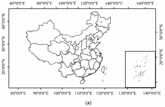
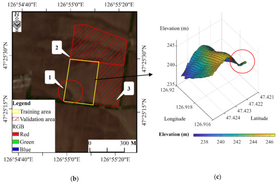
Figure 1.
Study area (a): The location of study area in China (red point); (b): Location of the study site (1) and validation site (2, 3); (c): Three-dimensional plot of the topography of the study; the red circle in Figure 1c corresponds to the red circle in Figure 1b, indicating the three-dimensional structure of the erosion ditch and the spatial location of the erosion ditch, respectively.
2.2. Topography Data Acquisition and Preprocessing
The DEM data used in this study include three different kinds: SRTM data, DEM data extracted from optical stereo-images (ZY-3 DEM) and UAV DEM data. Although SRTM data are vertically referenced to the EGM96 geoid, the Chinese elevation datum is the 1985 national elevation datum. Different elevation datums will lead to vertical deviations in DEM data. Therefore, we converted the SRTM data to the 1985 elevation datum and performed projection, horizontal and vertical corrections.
2.2.1. SRTM
The SRTM project is a joint endeavour of the National Aeronautics and Space Administration (NASA), the National Geospatial-Intelligence Agency, and the German and Italian Space Agencies, and it was launched in February 2000. The SRTM uses dual radar antennas to acquire interferometric radar data, which are processed to obtain digital topographic data; the corresponding data set includes the most complete, high-resolution DEM data for the Earth. SRTM data were downloaded (http://earthexplorer.usgs.gov/) and clipped to the extent of the study area. Studies have shown that low-pass filtering can remove known random speckle noise in SRTM data [21]. Therefore, the SRTM data was processed by a low-pass filter (SRTM low-pass filter, SRTM_LOW). In addition, the PSR in June, July, August and September were extracted from SRTM as the input variables of the improved SRTM DEM model.
2.2.2. DEM based on Optical Stereo Image Extraction (ZY3 DEM)
In this paper, optical stereo images at the 1C level were obtained on 12 May 2018. The geographical range was 126°31′11″–127°23′25″E and 47°6′20″–47°25′26″N. The data quality was high, and the cloud content was 0%. The texture and geometric structure of the land surface were clear. The front and back images of ZY-3 were used to cover the whole study area, and the overlap was 100%. To improve interpretability, the image was processed by colour stretching and image enhancement. Based on the ground control points and connection points, we extracted a DEM with a resolution of 5 m.
2.2.3. DEM based on Unmanned Aerial Vehicle (UAV DEM)
The DJI (DJ-Innovations) M600 Pro UAV (SZ DJI Technology Co., Shenzhen, China) was used as a remote sensing platform equipped with a RedEdge 3 camera (Table 1). The weather was clear and cloudless, and the wind speed was less than level 1 on 15 April 2018, reflecting suitable conditions for flight. The flying altitude was 110 m, and the actual altitude was 109.5 m. The filtered images and POS (Position and Orientation System) data were input into Pix4D mapper software, and we adjusted the processing parameters according to the configuration of the camera. After running the software, the application automatically generated the connection points and performed space-three calculations with the POS data, thereby obtaining precisely oriented elements and the coordinates of the encrypted points for each aerial image. After the point cloud was encrypted, the software automatically generated a digital surface model, which was used as the basis for digital differential correction to orthorectify each image. The vertical accuracy of the UAV DEM was verified to be 0.1 m based on actual ground points, so the UAV DEM was used as the reference DEM.

Table 1.
Technical specifications of unmanned aerial vehicle (UAV) and multispectral cameras.
Slope, aspect and solar radiation features were extracted from the UAV DEM by ArcGIS 10.2. By taking the north direction as zero degrees and dividing the slope direction every 45°, the southeastern and southern slopes were classified as sunny slopes, and the northwestern and northern slopes were classified as shady slopes. According to the actual situation in the study area, an area was considered flat when the slope was less than 1.5°, the area at the foot of the slope was larger than that at the bottom of the slope, and the slope classification zone (i.e., shady or sunny) was located between the top of the slope and the bottom of the slope (Figure 2). The topography of the study area was divided into ridge, shady, channel and sunny slope [22,23] classes to discuss the distribution of surface energy and materials (PDI, PSR, and NDVI) for different topographic features.
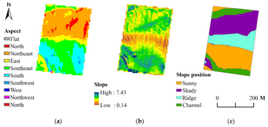
Figure 2.
The slope, aspect and position maps of the training area a ((a): aspect, (b): slope, and (c): slope position).
2.3. Remote Sensing Image Acquisition and Preprocessing
Cloud-free, orthorectified SPOT-6 (SPOT 6 is a satellite successfully launched by an Indian rocket PSLV-C21.) high-resolution geometric (HRG; 6 m × 6 m resolution) images acquired on 9 June, 9 July, 8 August and 3 September, 2016, were obtained (Table 2). ENVI 5.1 was used to perform radiometric calibration, atmospheric correction, and orthorectification, and ArcGIS 10.2 was used to clip the study area and calculate the NDVI [24]. Previous studies have shown that the PDI, which uses soil line, can effectively measure the characteristics of soil moisture in the surface layer [25]. Therefore, the Sentinel-2A image on 6 May 2016, was selected. Sentinel-2A provides L1C (LIC represents Level-1C, it is the Sentinel-2 product types. High-level description is the top of atmosphere reflectances in cartographic geometry.) atmospheric top-reflectance data processed by geometric correction, and only additional atmospheric correction is required. The atmospheric correction of the images was performed with SNAP software provided by the European Space Agency (ESA; atmospheric correction expands the reflectivity data set by 10,000 times). Bare soil images were used to obtain pure bare soil pixels, and the near-red and red bands were used to calculate the soil line. The corresponding expression is [25]:
where is near-red band reflectance; is red band reflectance; is the soil line slope; and I is the slope of a soil line at the ordinate.
Table 2.
Topography and Remote Sensing Data Acquisition and Processing.
The expression for calculating the PDI based on the soil line is as follows [25]:
2.4. Methodology
The study area was divided into three subareas for the experiments, and site 1 (an undulating region with erosion gullies; 2551 pixels) was used to train the improved SRTM model. Site 2 (1965 pixels) without erosion gullies and site 3 (3123 pixels) with erosion gullies were used as validation sites to assess the applicability of the improved SRTM method. Then, 13 variables related to the NDVI, PDI, PSR and SRTM in June, July, August and September were used as the input variables of the SLR model and BPNN model. In May 2016, field measurements were performed in the study area; an iRTK2 Global Positioning System (GPS) station with a positioning accuracy of a few centimetres was used. Precise coordinates and elevations were obtained to determine the accuracy of the UAV DEM. The UAV DEM and SRTM DEM were used as the reference DEM and input variable, respectively. In addition, the assessment of the resulting DEM included comparisons with the DEMs produced by a simple denoising method (SRTM_LOW) and commercially available optical stereo-images (ZY3 DEM).
2.4.1. Stepwise Linear Regression (SLR) Model
An SLR model was used to construct the relationship between input variables and the high-precision DEM. The SRTM data, NDVI, PSR and PDI in June, July, August and September were used as input variables in the SLR model. Variables that caused multicollinearity were filtered and removed. The SLR model can be expressed as follows [35,36]:
There is a constant term in the formula, and is the regression coefficient, is the independent variable and is the residual. The SLR model was implemented in SPSS statistics 22.
2.4.2. Back Propagation Neural Network (BPNN) Model
A BPNN is a multilayer feed-forward neural network composed of an input layer, a hidden layer and an output layer. It is a training algorithm that includes two processes. The first one is to feed forward the values to generate output. The second one is to calculate the error between the output and the target output, then back propagate this error to the lower layers, to update both weight matrices and bias vectors. The BPNN algorithm has high self-learning potential and wide applicability, thus, it is an effective method for solving nonlinear problems [14,37]. When establishing the BPNN prediction model, trainlm was selected as the training function, and sigmoid and purelin were selected as the transfer functions of the hidden layer and output layer, respectively; after many training steps, the numbers of nodes in the hidden layer and output layer were set as 1 and 1, respectively.
2.5. Assessment
According to the improved method, the spatial model similarity between the high-precision DEM and the reference DEM was evaluated based on the root mean square error (RMSE), correlation coefficient (R2) and bias [12]. As shown in Formulas (4)–(6), in addition to the comparison with the reference digital elevation model (UAV DEM), the high-precision DEM was also compared with SRTM_LOW and ZY-3 DEM.
where is the evaluated DEM elevation at pixel, is the reference DEM elevation at pixel , and is the total number of pixels.
3. Results
3.1. The Relationship between Topography and NDVI, PSR and PDI
The three-dimensional (3D) spatial distributions of topographic factors and the NDVI, PSR and PDI in June, July, August and September are shown in Figure 3 and Figure 4. Aspect was closely related to PSR because according to Figure 3b, Figure 2a and Figure 4e–h, the potential solar radiation in the north, northwest and northeast directions was lower than that in the south, southwest and southeast slopes in June, July, August and September. In addition, from July to September, the spatial differences in the PDI in areas with large topography fluctuations and high slopes are significant, and the soil moisture in these areas is generally higher than that in flat areas. Table 3 presents the correlation analysis results for the topography and input variables. The correlation coefficient between the NDVI and topography in June was only −0.023. There was no significant difference in the NDVI for different topographic features in June, mainly because soybean crops were in the early stage of emergence and jointing. Moreover, the study area was a black soil area, the soil was fertile, and the rainfall total was sufficient. The growth of crops mainly depends on the natural fertility of the soil, so the topography had little effect on the growth of crops in June. In July, soybean began to enter the flowering stage, the NDVI at different positions varied, and the growth difference gradually increased. As shown in Figure 3 and Figure 4e–h, although the spatial pattern of solar radiation from June to September was similar, the NDVI remained heterogeneous. Therefore, the PSR was not the main factor that caused the low NDVI. Notably, this trend was caused by topography and the soil erosion in cultivated land areas (Figure 1) [38,39] (e.g., there is an obvious erosion gully at longitude 123.916 and latitude 47.22 in Figure 3). The correlation between the PDI and soil moisture was negative, and the PDI was low at that area, indicating that the soil moisture was high. The groundwater in the area near the erosion gully underwent seepage, and water collected at the bottom of the erosion gully, resulting in excessive soil moisture in the erosion gully. In addition, erosion by water at the surface greatly reduced the organic matter and microbial contents of the soil, which limited the development of the biological components and internal structure of soybean. Therefore, the soybean grew slowly, and the NDVI in the plant canopy was low (Figure 4b). In addition, the NDVI in July was negatively correlated with topography (−0.327, p < 0.01), which further indicated that the effect of topography on surface moisture inhibits crop growth. However, when soybeans entered the scab stage in August, a large amount of moisture was needed. At this time, there was a positive correlation between the NDVI and topography (0.162, p < 0.01). This result indicated that the effect of topography on surface moisture in August promoted crop growth. Although the coefficient of variation (CV) of the NDVI in August (0.017) was less than that for the NDVI in July (0.024), the crop growth was relatively uniform, and waterlogging was still observed in erosion gullies with large slopes and topographic fluctuations. When soybean was in the full ripening stage (September), the crop components still contained a large amount of chlorophyll, and the contents of lutein and anthocyanin were low. At this time, the spectral response pattern of crops was similar to that in the peak growth period; thus, the NDVI was relatively high. These results demonstrated that the NDVI was closely related to topography and affected by surface matter during the crop growth period. Therefore, the spatiotemporal relationship between crops and topography was used to improve the SRTM DEM.
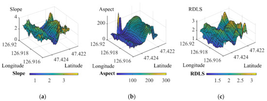
Figure 3.
Spatial distribution characteristics of topographic factors ((a): slope; (b): aspect; (c): relief degree of the land surface (RDLS)).
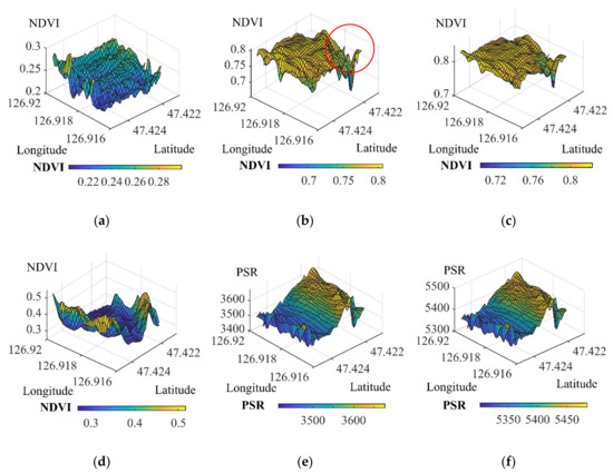
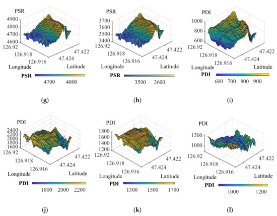
Figure 4.
Normalized differential vegetation index (NDVI), potential solar radiation (PSR) and perpendicular drought index (PDI) spatial distributions from June to September ((a–d) represent the June, July, August, and September NDVIs; (e–h) represent the June, July, August, and September PSRs; (i–k), and (l) represent the June, July, August, and September PDIs, respectively).
Table 3.
Correlation coefficient between topography and variables from June to September.
Figure 5 reflected the interaction between PSR and the PDI for different topographic characteristics in June, July, August and September. PSR and the PDI increased initially and then decreased from June to September. Figure 6 shows the rainfall and temperature data from June to September, and the trends are consistent with the phenological characteristics in Northeast China. From June to September, the distribution of PSR was uniform, and the difference in incident illuminance was low among different topographies, but the CV of soil moisture was significantly different at different slope positions (Table 4); this finding suggested that topography was an important factor that influenced the PDI. In Table 4, there was no significant difference in NDVI CV among different slope positions in June, and the crop growth was uniform. However, the CV of NDVI between different slope positions in July was greater than that of NDVI between different slope positions in June. The CV of NDVI on the shady slope was the largest, and there were obvious spatial differences in crop growth. When the crop entered the scab stage in August, the CV of NDVI was the smallest and the growth was the best. In September the crop matured gradually, and the CV of NDVI among different slope positions was significantly higher than that in August. However, crops on shady slopes grow poorly in July and August, which delayed the growth period of crops. Therefore, the CV of NDVI in shady slopes was the smallest in September. To sum up, topography is also an important factor affecting crop growth.
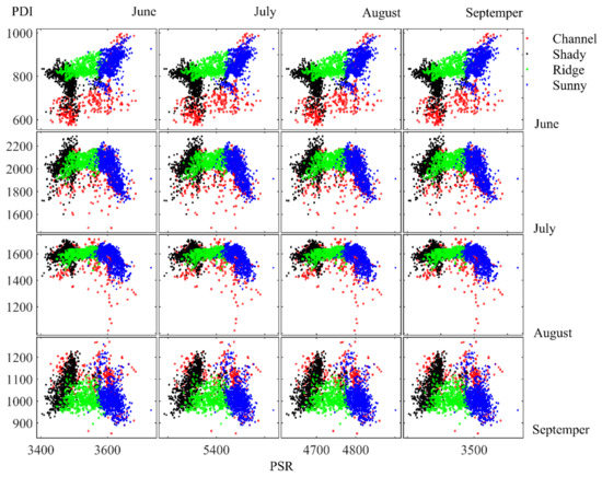
Figure 5.
Scatter plot of PDI and PSR at different slope positions.
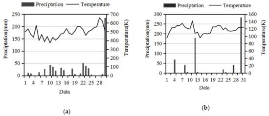
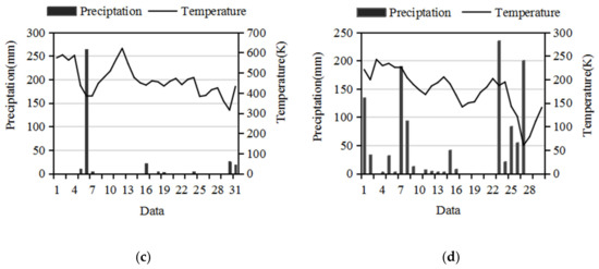
Figure 6.
Daily average temperature and rainfall in the study area. ((a–d) represent the rainfall and temperature in June, July, August and September, respectively.)
Table 4.
Statistical table of coefficient of variation (CV) of normalized differential vegetation index (NDVI), perpendicular drought index (PDI) and potential solar radiation (PSR).
3.2. Improving SRTM Data with the SLR and BPNN Models
The SRTM data and PSR in June and July and the NDVI in June, July and September were used as variables in the SLR model. Table 2 shows the detailed parameters of the SLR model. The unstandardized coefficient indicated that the inclusion of auxiliary variables improved the SRTM data. The correlation coefficients of the NDVI in June, July and September were −17.674, 3.532 and 2.610, respectively (Table 5), thus suggesting that the NDVI is an important variable for improving the SRTM DEM; conversely, the correlations between the SRTM data and PSR in June and July were low. This finding indicated that the influence of topography on the NDVI varies from June to September. Moreover, the significance of all independent variables used in the calculation was less than 0.01 (Table 3). This result was statistically verified.
Table 5.
Stepwise multivariate regression model analysis.
In the BPNN method, after repeated training, it was determined that the best number of nodes in the hidden layer was 1. The R2 value of the BPNN model was higher than that of the SLR model in Table 6. In addition, the accuracy of the two models was higher than that of ZY3 DEM and SRTM_LOW at both the modelling site and the validation site, thus improving the accuracy of the SRTM data. This finding indicates that the selection of input variables is objective and accurate.
Table 6.
Accuracy evaluation of different models at the training site.
3.3. Test Site Evaluation
As shown in Table 6, the R2 and RMSE of the BPNN method were 0.980 and 0.54 m, respectively, and the R2 and RMSE of the SLR method were 0.918 and 1.00 m, respectively. The results demonstrated that the model accuracy after BPNN training was higher than that based on the SLR model; thus, the BPNN model was used to improve the SRTM data at sites 2 and 3. Figure 7 shows the spatial distribution of different DEMs at site 2, including the generated high-precision DEM, UAV DEM, SRTM DEM, SRTM_LOW and ZY3 DEM. As assessed based on the spatial pattern, the generated high-precision DEM was consistent with the UAV DEM and yielded a significant improvement over the original SRTM DEM. Table 7 indicates that the error of the improved SRTM DEM using both linear and nonlinear models was significantly lower than that of the original SRTM DEM, SRTM_LOW and ZY3 DEM. The RMSE of the improved SRTM decreased significantly from 15.25 for the original SRTM DEM to 0.94 m, thus accounting for approximately 93% of the improvement at site b. Moreover, the RMSE and bias were better than those for SRTM_LOW (RMSE of 15.25 m and bias of 0.93) and ZY3 DEM (RMSE of 5.01 m and bias of 0.97).
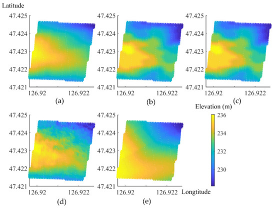
Figure 7.
Comparisons of DEMs at site 2: (a) unmanned aerial vehicle digital elevation model (UAV DEM); (b) Shuttle Radar Topography Mission digital elevation model (SRTM DEM); (c) SRTM low-pass filter (SRTM_Low); (d) Improved SRTM and (e) optical stereo-images (ZY3 DEM).
Table 7.
Accuracy evaluation of different digital elevation models (DEMs) at testing sites.
Figure 8 shows the spatial distribution of different DEMs at site 3, including the generated high-precision DEM, UAV DEM, SRTM DEM, SRTM_LOW and ZY3 DEM. Both the high-precision DEM generated and the reference UAV DEM showed the specific location of the erosion gully. Therefore, the generated high-precision DEM was most consistent with the UAV DEM and yielded a significant improvement over the original SRTM DEM. Moreover, the RMSE of the high-precision DEM decreased significantly from 14.95 for the original SRTM DEM to 1.23 m, thus resulting in an approximately 91% improvement at site c; additionally, the RMSE and bias were better than those for SRTM_LOW (RMSE: 14.95 m and bias: 0.93) and ZY3_DEM (RMSE: 3.41 mand bias: 0.98). The accuracy of the generated DEM in both the non-erosion gully undulating region 2 and erosion gully undulating region 3 further validated the applicability of the method.
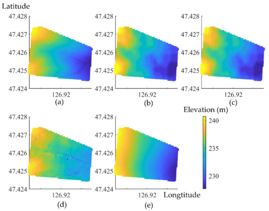
Figure 8.
Comparisons of DEMs at site 3: (a) UAV DEM; (b) SRTM DEM; (c) SRTM_Low Pass Filter; (d) Improved SRTM and (e) ZY3_DEM.
4. Discussion
4.1. Comparison of SLR and BPNN Model Performance in Improving the SRTM DEM
In this study, the NDVI in June, July, August and September and the variables that influence crop growth were used to improve the SRTM DEM in the study area via the linear SLR and nonlinear BPNN methods. Notably, the relationships among topography, crops and the factors that influence crop growth were assessed. The BPNN displayed the optimal ability to improve the SRTM data by providing sufficient useful information. Similar conclusions were reported by Wendi et al. [12], who improved SRTM data using data mining techniques and found that an MLP neural network was the best method of improvement. In contrast, the SLR model performed slightly worse than the others because it was based on traditional linear regression. Kulp et al. [9] demonstrated that the performance of a BPNN model was better than that of an SLR model, potentially because the DEM was affected by multifactor synthesis and was not as effective as the neural network in solving nonlinear problems.
The performance of the SLR model was slightly lower than that of the BPNN. This finding is associated with the collinearity among the predictors. Although the input variables can reflect the environmental characteristics that influence crop growth from different perspectives in this study, based on the relatively fixed spectral characteristics and response mechanism of soybean, the extracted vegetation feature information will inevitably have a certain degree of collinearity. Moreover, in the complex field environment, crop growth is determined by the interactions among various soil-influencing factors. Therefore, it is inevitable that there will be multicollinearity among the environmental factors that affect plant growth. In the SLR model, the collinearity problem was assessed through multicollinearity diagnosis and the variance inflation factor (VIF), as shown in Table 8. In principle, VIF > 10 indicates a collinearity problem [40]. The VIFs of PSR6 (VIF: 1098.460) and PSR7 (VIF: 1110.645) were higher than 10, indicating that the SLR model had a collinearity problem. Thus, the stability of the SLR model was poor.
Table 8.
Variance inflation factors (VIFs) for the stepwise linear regression (SLR) model.
4.2. Exploring the Relationship between Topography and the Crop Growth Mechanism
This study included two main findings. According to the relations among topography, crops, and the corresponding environmental factors, the feasibility of using different variables as inputs to improve the SRTM DEM was discussed. The applicability of this method was assessed via validation studies at sites 2 and 3, and a fast method of obtaining a high-precision DEM was provided for plain undulating regions.
At present, scholars have extensively studied the relationship between topography and solar radiation, topography and NDVI, and topography and soil moisture [28,41,42,43]. However, the comprehensive effects of these factors have not been fully explained. Thus, this paper mainly explored the comprehensive relationship among of these factors. As shown in Figure 4a–d, even in plain areas, there are still significant differences in crop growth within cultivated land zones. To explore the relationship between topography and crop growth in detail, according to the description in Section 2.2.3, training site a (UAV DEM) was divided into four regions: channel, shady, ridge and sunny regions. The CV of the NDVI reflected the uniformity of growth. In the process of crop ripening, whether in the whole training area or at different slope positions, the spatial CV of the NDVI displayed the following order: September (0.198) > June (0.058) > July (0.024) > August (0.017). The discreteness of the spatial distribution of PSR and the PDI at different slope positions (Figure 5) was associated with the increase in the NDVI CV in September. At different slope positions, the spatial evolution of the PDI and PSR from aggregation to discretization influenced the spatial distribution characteristics of the NDVI. Crop growth gradually transitioned from uniform to heterogeneous. Moreover, the PDI and PSR at the bottoms of slopes were larger than those at other slope positions, the CV of the NDVI at the bottoms of slopes was the largest, and crop growth was heterogeneous at different slope positions; these trends reflected the relation between topography and the PDI, PSR and NDVI. When the vegetation cover type was the same, the temporal and spatial variations in the NDVI were affected by two dominant factors: moisture and heat [16]. Additionally, topography was the key factor that influenced many environmental variables (e.g., moisture, temperature, and solar radiation) [17]. Therefore, the NDVI, PDI and PSR in June, July, August and September were introduced to improve the SRTM DEM, and the results displayed satisfactory accuracy at validation sites 2 and 3.
4.3. The Significance and Limitations of Research
In this study, according to the relationship between topography and crops, the NDVI and auxiliary data (PSR and PDI) were selected as inputs to improve the SRTM data. The results of this study were obtained in a temperate continental climate and a hilly black soil region, and they provide a reference for obtaining high-precision DEMs in similar climate areas. If we want to expand the area of the improved SRTM DEM, we can train high-precision DEMs in a small area and use the SRTM DEM for inversion to obtain regional-scale, high-precision DEM products. However, it must be noted that this methodology would require a reference DEM with similar land cover characteristics and a climatic area in which crops are planted once a year. Such land cover characteristics can be visibly identified using Google Earth imagery. Although the proposed method has certain practical value in filling the gaps in DEM data, it can still be improved. First, the environmental variables extracted from high-quality remote sensing images may produce better accuracy than the considered variables. Second, the relationship between topography and the surface material cycle can be further explored in the future, including the relation between soil nutrients and topography. Third, we comprehensively combined the time series characteristics of multiple important variables to improve SRTM data and increase the general applicability of the proposed model.
5. Conclusions
This study presented a new method for improving the accuracy of SRTM DEMs in cultivated land areas. According to the relationship between topography and crop growth in cultivated land areas, input variables were selected as auxiliary factors to improve SRTM data, and linear SLR and nonlinear BPNN models were used for training. The trained models were validated at sites 2 and 3 to validate the applicability of the method. Finally, the improved SRTM DEM was compared with the ZY-3 DEM and high-precision UAV DEM.
- (1)
- The results show that topography affects the redistribution of surface matter (solar radiation, temperature, and soil moisture) and the growth of crops in cultivated land areas. The introduction of the PDI, PSR and NDVI in the growing period can improve the accuracy of SRTM data.
- (2)
- The result of nonlinear fitting was better than that of linear fitting, and a BPNN was the best method for improving the accuracy of SRTM data. At validation sites 2 and 3, the R22 of the BPNN was 0.940, R23 was 0.920, RMSE2 was 0.94 m, and RMSE3 was 1.23 m. The accuracy at the two sites was improved by 93% and 91% compared with that obtained with the original SRTM DEM, respectively, and the spatial resolution was reduced to 1/5 times that of the original SRTM.
- (3)
- At validation sites 2 and 3, the accuracy of the DEM obtained by the proposed method was higher than that of the ZY-3 DEM and SRTM_LOW. This finding reflects the characteristics of erosion gullies in the study area. The spatial pattern of the DEM obtained by the proposed method was similar to that of the UAV DEM, which was close to the real surface pattern. Thus, the proposed method is suitable for areas with erosion gullies and undulations in plains.
Finally, this study provided an effective example for obtaining high-precision DEMs in cultivated land areas. The NDVI, PSR and PDI sequences exhibited excellent potential for improving SRTM data during the crop growth period. The proposed method improved the spatial resolution and vertical accuracy of SRTM data, enhanced the application value of SRTM DEMs and increased the overall understanding of the spatial characteristics of DEMs. This approach can be used to optimize the intelligent control of agricultural areas of production, such as by managing fertilizer and chemical treatments.
Author Contributions
Conceptualization, Y.M. and H.L.; methodology, Y.M.; software, Y.M.; validation, Y.M. and H.G.; formal analysis, Y.M. and H.G.; investigation, Y.Y. and M.W.; resources, F.K. and M.W.; data curation, Y.M.; writing—Original draft preparation, Y.M.; writing—Review and editing, M.X., Y.Y., L.M. and H.L.; visualization, M.X. and Y.C.; supervision, H.L.; project administration, B.J.; funding acquisition, B.J. All authors have read and agreed to the published version of the manuscript.
Funding
This research was funded by the “National Key R&D Program of China (2017YFD0201803)”; the Science and Technology Development Program of Jilin Province (No. 20200301014RQ).
Conflicts of Interest
The authors declare they have no known competing financial interest or personal relationships that could have appeared to influence the work reported in this paper.
References
- Gu, Z.; Xie, Y.; Gao, Y.; Ren, X.; Cheng, C.; Wang, S. Quantitative assessment of soil productivity and predicted impacts of water erosion in the black soil region of northeastern China. Sci. Total Environ. 2018, 637, 706–716. [Google Scholar] [CrossRef] [PubMed]
- Rodriguez, E.; Morris, C.S.; Belz, J.E. A global assessment of the SRTM performance. Photogramm. Eng. Remote Sens. 2006, 72, 249–260. [Google Scholar] [CrossRef]
- Nie, X.; Guo, W.; Huang, B.; Zhuo, M.; Li, D.; Li, Z.; Yuan, Z. Effects of soil properties, topography and landform on the understory biomass of a pine forest in a subtropical hilly region. Catena 2019, 176, 104–111. [Google Scholar] [CrossRef]
- Yang, Q.-Y.; Jiang, Z.-C.; Li, W.-J.; Li, H. Prediction of soil organic matter in peak-cluster depression region using kriging and terrain indices. Soil Tillage Res. 2014, 144, 126–132. [Google Scholar] [CrossRef]
- Bracke, M.S.; Miller, C.C.; Kim, J. Adding value to digitizing with GIS. Library Hi Tech. 2008, 26, 201–212. [Google Scholar] [CrossRef]
- Long, J.; Liu, Y.; Xing, S.; Qiu, L.; Huang, Q.; Zhou, B.; Shen, J.; Zhang, L. Effects of sampling density on interpolation accuracy for farmland soil organic matter concentration in a large region of complex topography. Ecol. Indic. 2018, 93, 562–571. [Google Scholar] [CrossRef]
- Wasklewicz, T.; Staley, D.M.; Reavis, K.; Oguchi, T. 3.6 Digital Terrain Modeling. In Treatise on Geomorphology; Shroder, J.F., Ed.; Academic Press: San Diego, CA, USA, 2013; pp. 130–161. [Google Scholar] [CrossRef]
- Zhang, W.; Qi, J.; Wan, P.; Wang, H.; Xie, D.; Wang, X.; Yan, G. An Easy-to-Use Airborne LiDAR Data Filtering Method Based on Cloth Simulation. Remote Sens. 2016, 8, 501. [Google Scholar] [CrossRef]
- Kulp, S.A.; Strauss, B.H. CoastalDEM: A global coastal digital elevation model improved from SRTM using a neural network. Remote Sens. Environ. 2018, 206, 231–239. [Google Scholar] [CrossRef]
- Bhardwaj, A.; Jain, K.; Chatterjee, R.S. Generation of high-quality digital elevation models by assimilation of remote sensing-based DEMs. J. Appl. Remote Sens. 2019, 13. [Google Scholar] [CrossRef]
- Ajibola, I.I.; Mansor, S.; Pradhan, B.; Shafri, H.Z.M. Fusion of UAV-based DEMs for vertical component accuracy improvement. Measurement 2019, 147. [Google Scholar] [CrossRef]
- Wendi, D.; Liong, S.-Y.; Sun, Y.; Doan, C.D. An innovative approach to improve SRTM DEM using multispectral imagery and artificial neural network. J. Adv. Model. Earth Syst. 2016, 8, 691–702. [Google Scholar] [CrossRef]
- Manry, M.T.J.N.N. Adaptive pattern recognition and neural networks. Neural Netw. 1991, 4, 124–126. [Google Scholar] [CrossRef]
- Zhong, W.; Deng, Y.; Tenreiro Machado, J.A.; Zhang, C.; Zhao, K.; Wang, X. Strength prediction of similar materials to ionic rare earth ores based on orthogonal test and back propagation neural network. Soft Comput. 2019, 23, 9429–9437. [Google Scholar] [CrossRef]
- Estes, L.D.; Reillo, P.R.; Mwangi, A.G.; Okin, G.S.; Shugart, H.H. Remote sensing of structural complexity indices for habitat and species distribution modeling. Remote Sens. Environ. 2010, 114, 792–804. [Google Scholar] [CrossRef]
- Guo, L.; Linderman, M.; Shi, T.; Chen, Y.; Duan, L.; Zhang, H. Exploring the Sensitivity of Sampling Density in Digital Mapping of Soil Organic Carbon and Its Application in Soil Sampling. Remote Sens. 2018, 10, 888. [Google Scholar] [CrossRef]
- Riihimäki, H.; Heiskanen, J.; Luoto, M. The effect of topography on arctic-alpine aboveground biomass and NDVI patterns. Int. J. Appl. Earth Obs. 2017, 56, 44–53. [Google Scholar] [CrossRef]
- Western, A.W.; Zhou, S.L.; Grayson, R.B.; McMahon, T.A.; Bloschl, G.; Wilson, D.J. Spatial correlation of soil moisture in small catchments and its relationship to dominant spatial hydrological processes. J. Hydrol. 2004, 286, 113–134. [Google Scholar] [CrossRef]
- Batlles, F.J.; Bosch, J.L.; Tovar-Pescador, J.; Martinez-Durban, M.; Ortega, R.; Miralles, I. Determination of atmospheric parameters to estimate global radiation in areas of complex topography: Generation of global irradiation map. Energy Convers. Manag. 2008, 49, 336–345. [Google Scholar] [CrossRef]
- Bosch, J.L.; Baffles, F.J.; Zarzalejo, L.F.; Lopez, G. Solar resources estimation combining digital terrain models and satellite images techniques. Renew. Energy 2010, 35, 2853–2861. [Google Scholar] [CrossRef]
- Stevenson, J.A.; Sun, X.; Mitchell, N.C. Despeckling SRTM and other topographic data with a denoising algorithm. Geomorphology 2010, 114, 238–252. [Google Scholar] [CrossRef]
- Dragut, L.; Blaschke, T.J.G. Automated classification of landform elements using object-based image analysis. Geomorphology 2006, 81, 330–344. [Google Scholar] [CrossRef]
- Skidmore, A.K. Terrain position as mapped from a gridded digital elevation model. Int. J. Geogr. Inf. Syst. 1990, 4, 33–49. [Google Scholar] [CrossRef]
- Dou, X.; Wang, X.; Liu, H.; Zhang, X.; Meng, L.; Pan, Y.; Yu, Z.; Cui, Y. Prediction of soil organic matter using multi-temporal satellite images in the Songnen Plain, China. Geoderma 2019, 356, 113896. [Google Scholar] [CrossRef]
- Zhan, Z.; Qin, Q.; Ghulan, A.; Wang, D. NIR-red spectra space based new method for soil moisture monitoring. Sci. China Earth Sci. 2007, 50, 283–289. [Google Scholar] [CrossRef]
- Yang, H.; Zhang, X.; Xu, M.; Shao, S.; Wang, X.; Liu, W.; Wu, D.; Ma, Y.; Bao, Y.; Zhang, X.; et al. Hyper-temporal remote sensing data in bare soil period and terrain attributes for digital soil mapping in the Black soil regions of China. Catena 2020, 184, 104259. [Google Scholar] [CrossRef]
- Goulden, T.; Hopkinson, C.; Jamieson, R.; Sterling, S. Sensitivity of DEM, slope, aspect and watershed attributes to LiDAR measurement uncertainty. Remote Sens. Environ. 2016, 179, 23–35. [Google Scholar] [CrossRef]
- Blal, M.; Khelifi, S.; Dabou, R.; Sahouane, N.; Slimani, A.; Rouabhia, A.; Ziane, A.; Neçaibia, A.; Bouraiou, A.; Tidjar, B. A prediction models for estimating global solar radiation and evaluation meteorological effect on solar radiation potential under several weather conditions at the surface of Adrar environment. Measurement 2020, 152, 107348. [Google Scholar] [CrossRef]
- Miyasaka, T.; Kulkarni, A.; Kim, G.M.; Oz, S.; Jena, A.K. Perovskite Solar Cells: Can We Go Organic-Free, Lead-Free, and Dopant-Free? Adv. Energy Mater. 2020, 10. [Google Scholar] [CrossRef]
- Wang, M.; Zhu, Y.; Jin, S.; Pan, J.; Zhu, Q. Correction of ZY-3 image distortion caused by satellite jitter via virtual steady reimaging using attitude data. ISPRS J. Photogramm. 2016, 119, 108–123. [Google Scholar] [CrossRef]
- Ni, W.; Sun, G.; Ranson, K.J.; Pang, Y.; Zhang, Z.; Yao, W. Extraction of ground surface elevation from ZY-3 winter stereo imagery over deciduous forested areas. Remote Sens. Environ. 2015, 159, 194–202. [Google Scholar] [CrossRef]
- Maresma, A.; Chamberlain, L.; Tagarakis, A.; Kharel, T.; Godwin, G.; Czymmek, K.J.; Shields, E.; Ketterings, Q.M. Accuracy of NDVI-derived corn yield predictions is impacted by time of sensing. Comput. Electron. Agric. 2020, 169, 105236. [Google Scholar] [CrossRef]
- Li, C.; Li, H.; Li, J.; Lei, Y.; Li, C.; Manevski, K.; Shen, Y. Using NDVI percentiles to monitor real-time crop growth. Comput. Electron. Agric. 2019, 162, 357–363. [Google Scholar] [CrossRef]
- Shahabfar, A.; Ghulam, A.; Eitzinger, J. Drought monitoring in Iran using the perpendicular drought indices. Int. J. Appl. Earth Obs. 2012, 18, 119–127. [Google Scholar] [CrossRef]
- Kokaly, R.F.; Clark, R.N. Spectroscopic Determination of Leaf Biochemistry Using Band-Depth Analysis of Absorption Features and Stepwise Multiple Linear Regression. Remote Sens. Environ. 1999, 67, 267–287. [Google Scholar] [CrossRef]
- Zare, S.; Fallah Shamsi, S.R.; Abtahi, S.A. Weakly-coupled geo-statistical mapping of soil salinity to Stepwise Multiple Linear Regression of MODIS spectral image products. J. Afr. Earth Sci. 2019, 152, 101–114. [Google Scholar] [CrossRef]
- Vogl, T.P.; Mangis, J.K.; Rigler, A.K.; Zink, W.T.; Alkon, D.L. Accelerating the convergence of the back-propagation method. Biol. Cybern. 1988, 59, 257–263. [Google Scholar] [CrossRef]
- Gusarov, A.V. The response of water flow, suspended sediment yield and erosion intensity to contemporary long-term changes in climate and land use/cover in river basins of the Middle Volga Region, European Russia. Sci. Total Environ. 2020, 719. [Google Scholar] [CrossRef]
- Mamedov, A.I.; Levy, G.J. Soil erosion-runoff relations on cultivated land: Insights from laboratory studies. Eur. J. Soil. Sci. 2019, 70, 686–696. [Google Scholar] [CrossRef]
- O’Brien, R.M. A caution regarding rules of thumb for variance inflation factors. Qual. Quant. 2007, 41, 673–690. [Google Scholar] [CrossRef]
- Zhu, Q.; Lin, H. Influences of soil, terrain, and crop growth on soil moisture variation from transect to farm scales. Geoderma 2011, 163, 45–54. [Google Scholar] [CrossRef]
- Western, A.W.; Grayson, R.B.; Blöschl, G.; Willgoose, G.R.; Mcmahon, T.A.J.W.R.R. Observed spatial organization of soil moisture and its relation to terrain indices. Water Resour. Res. 1999, 35, 797–810. [Google Scholar] [CrossRef]
- Zhan, Z.-Z.; Liu, H.-B.; Li, H.-M.; Wu, W.; Zhong, B. The Relationship between NDVI and Terrain Factors-A Case Study of Chongqing. Procedia Environ. Sci. 2012, 12, 765–771. [Google Scholar] [CrossRef]
Publisher’s Note: MDPI stays neutral with regard to jurisdictional claims in published maps and institutional affiliations. |
© 2020 by the authors. Licensee MDPI, Basel, Switzerland. This article is an open access article distributed under the terms and conditions of the Creative Commons Attribution (CC BY) license (http://creativecommons.org/licenses/by/4.0/).