Quality Assessment of Photogrammetric Models for Façade and Building Reconstruction Using DJI Phantom 4 RTK

Abstract

Aerial photogrammetry by Unmanned Aerial Vehicles (UAVs) is a widespread method to perform mapping tasks with high-resolution to reconstruct three-dimensional (3D) building and façade models. However, the survey of Ground Control Points (GCPs) represents a time-consuming task, while the use of Real-Time Kinematic (RTK) drones allows for one to collect camera locations with an accuracy of a few centimeters. DJI Phantom 4 RTK (DJI-P4RTK) combines this with the possibility to acquire oblique images in stationary conditions and it currently represents a versatile drone widely used from professional users together with commercial Structure-from-Motion software, such as Agisoft Metashape. In this work, we analyze the architectural application of this drone to the photogrammetric modeling of a building with particular regard to metric survey specifications for cultural heritage for 1:20, 1:50, 1:100, and 1:200 scales. In particular, we designed an accuracy assessment test signalizing 109 points, surveying them with total station and adjusting the measurements through a network approach in order to achieve millimeter-level accuracy. Image datasets with a designed Ground Sample Distance (GSD) of 2 mm were acquired in Network RTK (NRTK) and RTK modes in manual piloting and processed both as single façades (S–F) and as an overall block (4–F). Subsequently, we compared the results of photogrammetric models generated in Agisoft Metashape to the Signalized Point (SP) coordinates. The results highlight the importance of processing an overall photogrammetric block, especially whenever part of camera locations exhibited a poorer accuracy due to multipath effects. No significant differences were found between the results of network real-time kinematic (NRTK) and real-time kinematic (RTK) datasets. Horizontal residuals were generally comparable to GNSS accuracy in NRTK/RTK mode, while vertical residuals were found to be affected by an offset of about 5 cm. We introduced an external GCP or used one SP per façade as GCP, assuming a poorer camera location accuracy at the same time, in order to fix this issue and comply with metric survey specifications for the widest architectural scale range. Finally, both S–F and 4–F projects satisfied the metric survey requirements of a scale of 1:50 in at least one of the approaches tested.

1. Introduction

The level of detail to achieve is a fundamental and crucial aspect [1,2] for the selection of the most suitable survey technique to adopt for urban remote sensing and landscape mapping [3,4]. A multitude of solutions can be adopted whenever a high detail is required to characterize buildings. Through the years, in fact, (i) direct survey with total station, (ii) combined use of terrestrial photogrammetry and total station, and (iii) Terrestrial Laser Scanning (TLS) with the possibility to acquire images of the instrument surroundings to colorize point clouds have been used to describe façades. However, not all of them could represent an optimal solution (especially for professional users) and the best choice should be evaluated case-by-case. The first method, for instance, is very time-consuming: every point must be surveyed with the instrument and it is almost impossible to survey everything. When the façades show higher level of complexity, due to architectural ornaments or friezes, the combination of terrestrial pictures and total station measurements can provide additional information; however, telescope rods should be used for tall buildings. In any case, it is hard to exceed a building altitude of ca. 10 m. Therefore, TLS represents a method to overcome this issue: in spite of a not negligible instrument cost (tens of thousands of euros), laser scanners are able to acquire up to millions of points per second [5,6]. The high density of final point clouds can be exploited for high-resolution façade mapping or inspection [7]. However, registration and processing of scans are also crucial aspects in an urban environment [8,9] and, nonetheless, the actual point grid step on a surface depends on the distance between the instrument and the surface itself, thus the level of detail at the top of a façade may be not sufficient to describe it adequately. Furthermore, out-of-plane elements, such as ornaments, friezes, and balconies, may cause shadows in laser scanning clouds. TLS and close-range photogrammetry can be integrated to overcome some of the issues above [10,11,12].

The use of Unmanned Aerial Vehicles (UAVs) as platforms to acquire image datasets for the mapping of buildings has been largely and successfully used in the last years for such purpose. Aerial photogrammetry by UAVs combines the advantage of (i) capturing images, (ii) generating dense point clouds, and (iii) a cost of about some thousands of euros and, thus, can represent an optimal solution [13,14]. Applications in the field of architectural and cultural heritage preservation are represented by the data acquisition for 3D modeling and assessment in emergency management [15,16], for ancient buildings [17] and in archeology [18,19,20]. Moreover, some authors have also used mini [21] and ultralight UAVs [22] that are considered to be harmless by national regulations [23].

A set of well-distributed Ground Control Points (GCPs) is usually needed to georeference the models. However, the survey of GCPs, generally performed using total stations, GNSS receivers or TLS, is a time-consuming task. The use of drones equipped with an on-board multi-frequency multi-constellation GNSS receiver used in Real-Time Kinematic (RTK), Network RTK (NRTK), or Post-Processing Kinematic (PPK) modes makes the use of direct georeferencing techniques with a centimeter-level accuracy of camera locations possible [24,25]. The most common field of application is the mapping of a broad land extent [26,27], with the subsequent production of orthomosaics and digital elevation models without the need for surveying a high number of GCPs [28,29,30]. In any case, whichever it is the GNSS kinematic mode adopted, the vertical accuracy of the photogrammetric models that were obtained is strongly related to a consistent estimate of the focal length of the camera, in particular, for nadiral datasets [31]. A single GCP allows for one to considerably reduce the vertical error of digital elevation models, as pointed out by Forlani et al. [32], as well as the introduction of a short sequence of oblique images during the image processing of nadiral datasets that were investigated by Taddia et al. [33].

The availability of lightweight RTK multi-copters, with the possibility to rotate the camera and to acquire images, even in a stationary situation (i.e., with a null speed of the aircraft), makes it possible to extend the use of direct georeferencing to further fields of application, such as the survey of building and façades. The recent DJI Phantom 4 RTK (DJI-P4RTK) is a drone that combines the possibility to acquire oblique images (due to the presence of a gimbal) with the advantages of using an on-board multi-frequency multi-constellation GNSS receiver in kinematic modes [31,34] and it has the requirements for applying direct georeferencing to the field of urban remote sensing. The combination of RTK image datasets with a Structure-from-Motion approach potentially allows for one to reconstruct detailed three-dimensional (3D) models and point clouds with a centimeter level of georeferencing accuracy [35,36,37].

In this work, we analyze the potential of DJI-P4RTK for the reconstruction of photogrammetric models performing an accuracy assessment test by using image datasets whose CC locations were acquired in RTK and NRTK. In a first step, no point surveyed by total station, geodetic GNSS receiver, or TLS was ever introduced during the creation of photogrammetric models. A set of Signalized Points (SPs), used as high quality check points, allowed for us to evaluate the final level of accuracy of the models with more precision than using natural points, since the test was designed with the aim to achieve a millimeter-level accuracy. The SPs, consisting in well-visible targets, were surveyed by total station and all the measurements were adjusted through a network approach. Focusing on professional users, photogrammetric models were generated while using Agisoft Metashape and varying the processing strategy both for single façades (S–F) or using the entire image dataset of the building as an overall block (4–F). The SP identification error on the images was also evaluated. In a second step, we introduced (i) an external GCP and (ii) four SPs (one per façade) as GCPs during image alignment to fix a vertical offset of the models that was noticed during the first step.

Therefore, the aim and novelty of this research is to evaluate the results achievable with the DJI-P4RTK drone and an Agisoft Metashape data processing in the field of building and façade modeling, instead of land mapping, like Forlani et al. [32], Kalacska et al. [38], Barba et al. [39], and Štroner et al. [37], through a rigorous set up of the assessment test. In this work, we designed the image acquisition acquiring also oblique images in order to avoid issues that are related to the estimation of a wrong focal length [32,33]. We investigated in detail whether metric survey specifications for cultural heritage for 1:20, 1:50, 1:100, and 1:200 scales were satisfied or not [40,41,42].

A description of the test-site and the unmanned aircraft is presented in Section 2.1 and Section 2.2. The signalization, survey and network adjustment of SPs with total station (and static GNSS) is reported in Section 2.3, while the image dataset acquisition is presented in Section 2.4. Finally, the generation of photogrammetric models, the computation of residuals, and absolute and relative Root Mean Square Errors (RMSE) are reported in Section 2.5. Similarly to the materials and methods, the results start from the analysis of SP identification error by two different operators (Section 3.1) and the analysis of input camera location accuracy (Section 3.2), continuing with the computation of horizontal and vertical SP residuals (Section 3.3) and absolute and relative RMSE (Section 3.4).

2. Materials and Methods

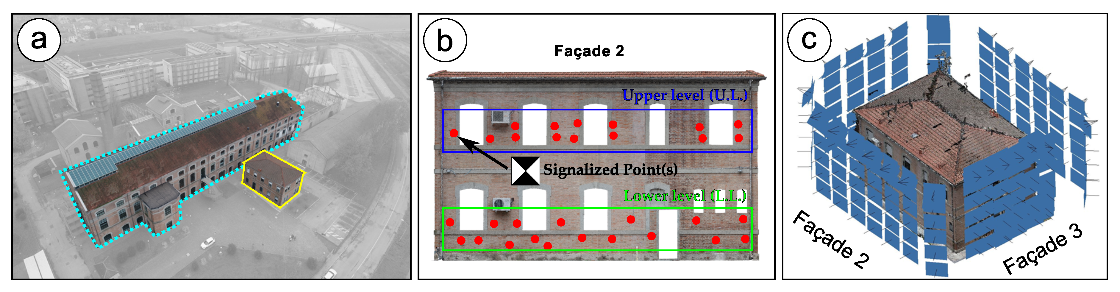
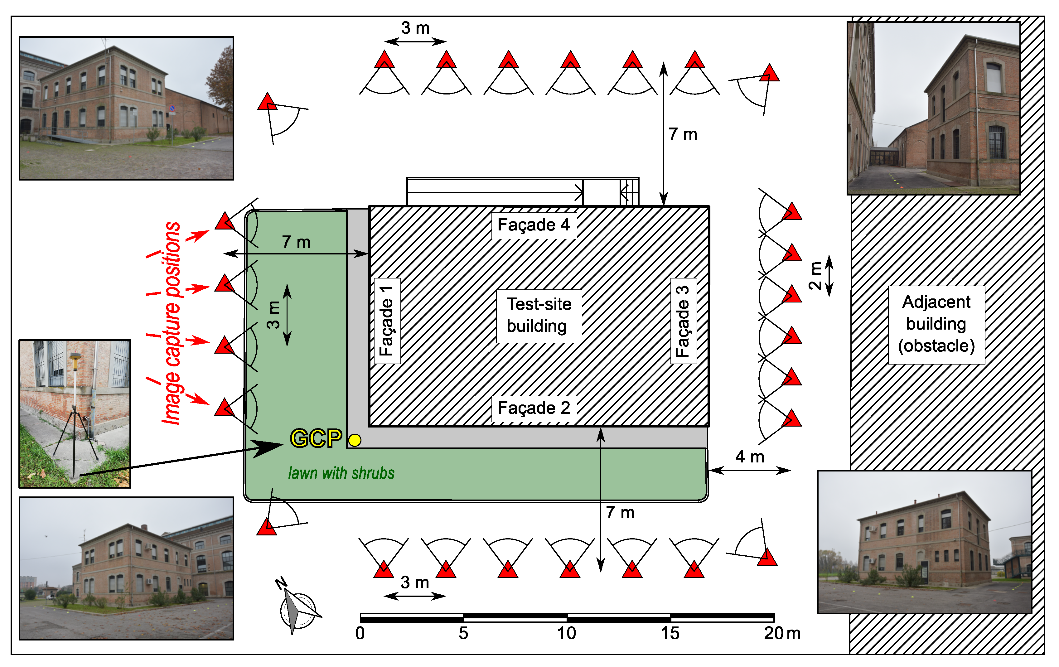
2.1. Test-Site Building

In this work, we selected a compact building with a rectangular shape (ca. $11\times 16$ m) and an height of about 9–10 m within the campus of the University of Ferrara as test-site. A second building (not surveyed) was located at a distance of 7 m from it, with a height of about 18–20 m (Figure 1a). In this way, we were able to fly around the test-site building easily and test a 4–F approach easily.

We deployed a total of 109 SPs on the external walls of the test-site building in order to signalize well-visible points and further collect their coordinates with a millimeter-level accuracy. SPs were placed on two different levels (one for each floor) and generally staggered whenever possible (Figure 1b). This allowed for us to realize a sort of quite regular and homogeneous point grid for each façade to proceed further with the validation and accuracy assessment of photogrammetric models (Figure 1c).

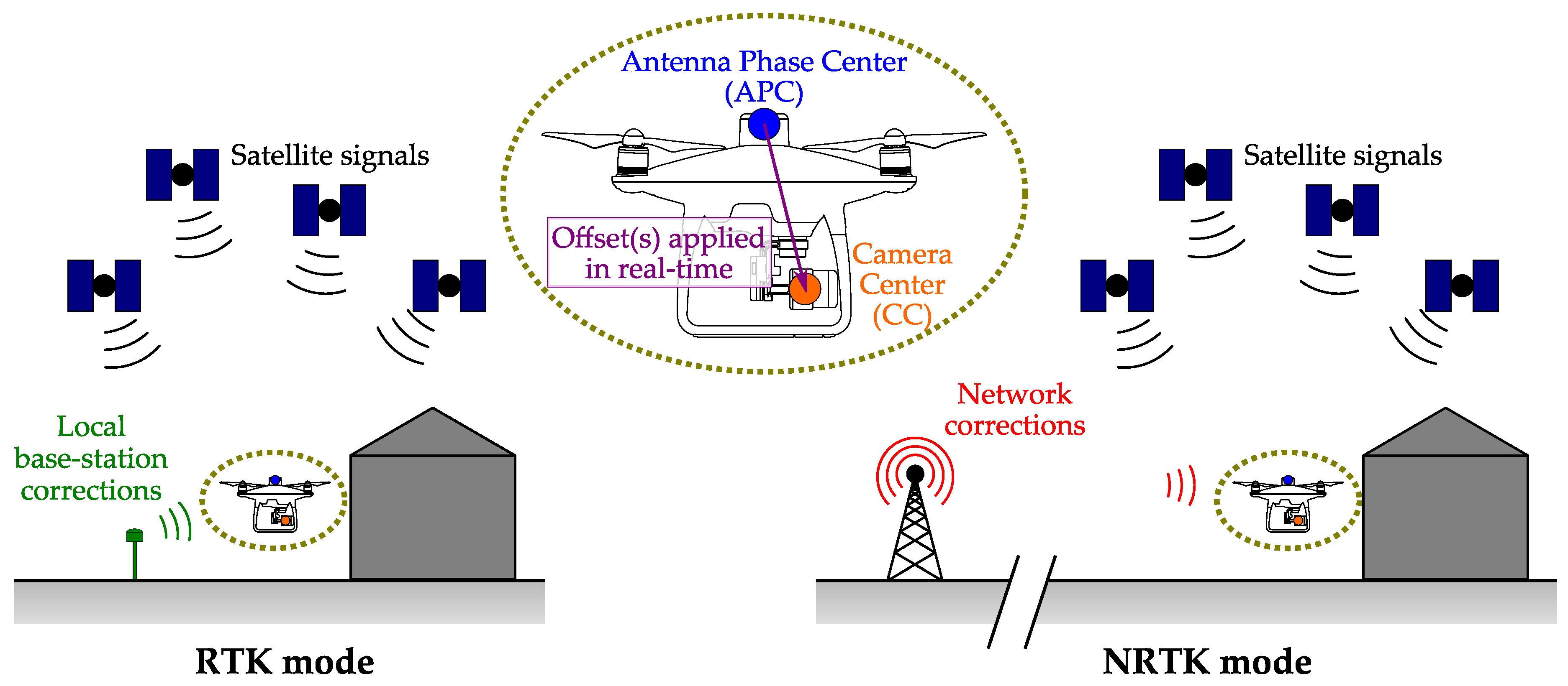
2.2. Unmanned Aircraft

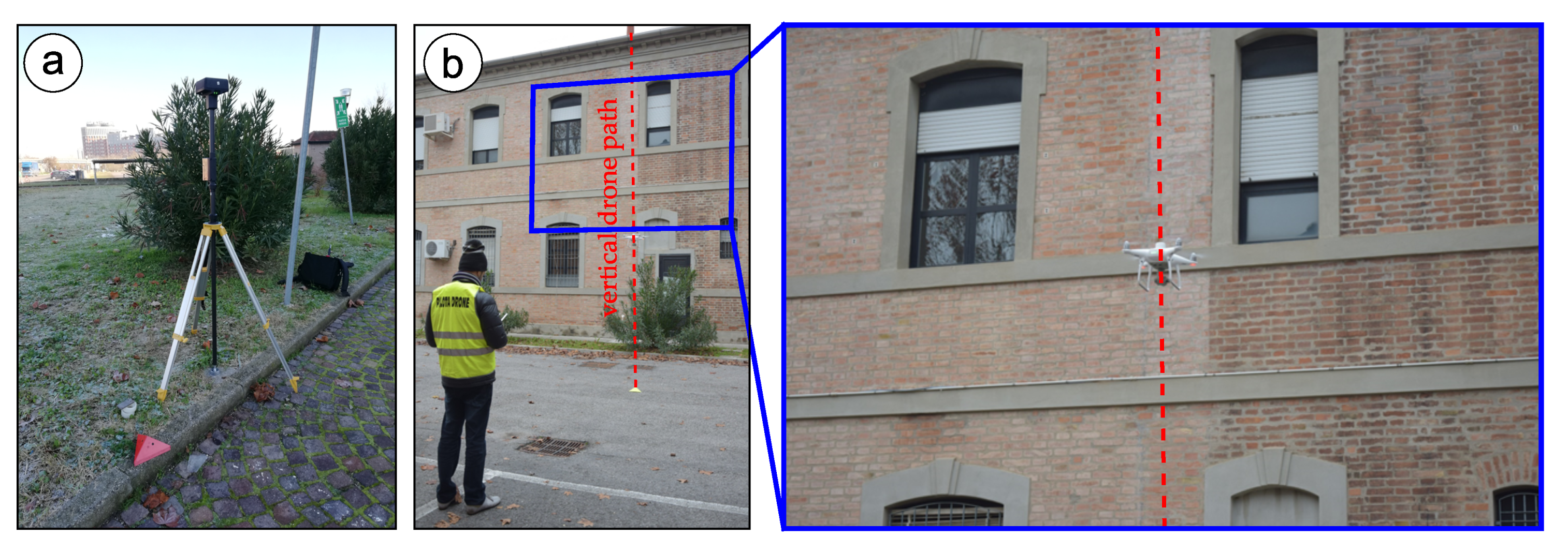
In this work, the aerial image datasets were acquired while using a recent model of RTK multi-copter: the DJI Phantom 4 RTK (DJI-P4RTK). Lightweight, versatility, and easy-to-use make this UAV a solution widely used by professional users in aerial photogrammetry currently. Moreover, its 20 Mpix camera with a gimbal allows one to acquire images in off-nadir positions. This aspect is crucial for mapping building façades, as well as the possibility to hovering.

The DJI-P4RTK is equipped with a multi-frequency multi-constellation GNSS receiver that is able to receive signals of GPS, GLONASS, BeiDou, and Galileo constellations [43]. The drone is ready to be used in RTK or in NRTK mode (positioning accuracy [43] is reported in

Table 1. Aircraft technical specifications.

Specifications
Horizontal positioning accuracy (${\sigma }_{H_{\mathrm{drone}}}$)	1.0 cm + 1 ppm (RMS)
Vertical positioning accuracy (${\sigma }_{V_{\mathrm{drone}}}$)	1.5 cm + 1 ppm (RMS)
Resolution	20 Mpix
Image Size	$5472\times 3648$
Field of View	84°
Focal Length	8.8 mm
Pixel Size	$2.4\mu m$
GSD @ 7.00 m	$\approx 1.9mm$
GSD @ 4.00 m	$\approx 1.1mm$

). We tested both approaches (Figure 2) by using a network service for receiving NRTK corrections and by setting up the DJI D-RTK 2 Mobile Station on a benchmark of known coordinates for RTK operations (Figure 3a). The management of the aircraft, as well as the configuration of NRTK and RTK operations (i.e., connection to the server for NRTK, link with the base receiver, imposition of base station coordinates), was carried out through the GS RTK app that is integrated into the remote controller of the DJI-P4RTK. The same app was also used for flying the drone and capturing images, even if no automatic mission was actually planned (Figure 3b). More details about the image dataset acquisition are given in Section 2.4.

During image capture, the DJI-P4RTK records the coordinates of the Camera Center (CC) location (along with the accuracy of the GNSS solution) into Exif metadata. Because of the presence of an Inertial Measurement Unit (IMU), in fact, the GNSS solution computed for the Antenna Phase Center (APC) of the on-board receiver is referred to the CC using yaw, pitch, and roll angles [33,43]. However, it is important to highlight here that system calibration [44,45] is a crucial aspect for reaching the maximum accuracy in computing Camera Center (CC) locations from the corresponding APC solutions [33]. In fact, APC–CC offsets have to be taken into account with a millimeter-level accuracy in order to preserve the quality of APC solutions. Using yaw, pitch, and roll angles that are continuously measured through the on-board IMU in real-time it is possible to computing RTK/NRTK camera locations (see Figure 2). In this way, the coordinates of the CC at the time of each image capture are known with a centimeter-level accuracy (in fixed NRTK/RTK solutions). Moreover, if a raw GNSS observation file is also recorded, then the flight path can also be computed in PPK mode [46]. Using timestamps recorded at the time of each image capture it is possible to interpolate flight path solutions computing APC solutions at the time of image acquisition [33].

2.3. Survey of SPs

2.3.1. In-Situ Operations

Prior to the materialization of SPs, we created a network made of four benchmarks (benchmarks in this work are S1, S2, S3, and S4 (see Figure 4)). The benchmarks have been placed close to the building corners. In this way, we were able to survey the SPs from two different benchmarks further with total station. Survey operations were carried out using a motor total station Topcon MSAX05II (${\sigma }_{\mathrm{angular}}=0.15$ mgon, ${\sigma }_{\mathrm{distance}}=0.8$ mm + 1 ppm using prism) and circular prism (60 mm aperture). This model of instrument is currently one of the most performing ones, having technical specifications that ensure the maximum level of accuracy in distance and angle measurements. Additionally, we adopted particular precautions during survey operations in order to limit any possible source of errors. Therefore, we never removed the tripod or the tribrach, but we exchanged total stations and prisms instead, remeasuring the instrument height. In this way, we avoided newer centering errors. Additionally, each measurement (i.e., slope distance, zenith angle, and horizontal angle) was repeated three times in both direct and reverse position and the average was recorded.

Because the DJI-P4RTK drone is equipped with an on-board GNSS receiver, operating in NRTK the antenna phase center of the aircraft is automatically framed within the official Italian reference system ETRS89 in its ETRF2000 (2008.0) realization, thus in ETRS89-ETRF2000 (2008.0). The same happens when introducing base receiver coordinates in ETRS89-ETRF2000 (2008.0) in RTK mode. The survey of the network in a local reference system would not allow us to compare SP coordinates with the photogrammetric model and we should introduce a datum transformation whose accuracy can affect the consistency of the comparison itself. For this reason, we decided to collect static GNSS data placing geodetic receivers (Topcon GR3, GPS+GLONASS, multi-frequency) on S1 and S4 (i.e., on the benchmarks with the clearest sky visual) with an occupation duration of about 2 h. In this way, we were able to frame our local survey performed with total station into ETRS89-ETRF2000 (2008.0) (see Section 2.3.2). In order to avoid possible vertical errors related, on one hand, to the measurement of the instrument height of total station and prisms and, on the other hand, to the Up component of GNSS systems, we also carried out a leveling with a Leica DNA03 level and a high-precision staff (non-extensible 3 m staff with bar code printed on an invar alloy strip). No plate was used due to the very limited distance between benchmarks.

Target signalization on the four building façades has been carried out only after the realization and survey of the network described above in order to preserve SPs. The use of natural points, i.e., non-signalized, would have not allowed us to reach a high level of accuracy during surveying and, in particular, while performing SP identification on the acquired images. Each SP consisted of a non-reflective target with a size of $30\times 30$ mm with a scale-independent pattern (see Figure 1b) that facilitated the further identification process. SP survey has been carried out in the days after the realization of the network and we used a Leica TS06 total station (${\sigma }_{\mathrm{angular}}=0.6$ mgon, ${\sigma }_{\mathrm{distance}}=2$ mm + 2 ppm in reflectorless mode) for this task. Each SP was surveyed by two different stations (i.e., benchmark positions) measuring in both direct and reverse position in order to assess the quality of measurements directly and ensure redundancy. We signalized and surveyed 18 points on Façade 1 (F. 1), 31 on Façade 2 (F. 2), 24 on Façade 3 (F. 3), and 36 on Façade 4 (F. 4). Additionally, the points were deployed on two different levels (one for each floor) and generally staggered, as already pointed out in Section 2.1. In the following, we will refer to levels as the lower (L.L.) and the upper ones (U.L.).

2.3.2. Post-Processing of GNSS Data

The post-processing of static GNSS data that were collected on benchmarks S1 and S4 was performed through Topcon Tools v.8.2.3. We downloaded the observations of the Continuously Operating Reference Station (CORS) FERR located at about 1 km away from our test-site location. FERR is framed into ETRS89-ETRF2000 (2008.0) and it belongs to the NetGEO (Topcon Positioning Italy) network, which is the same service that we used during NRTK mode. Moreover, we also introduced precise orbits (data downloaded from ftp://cddis.gsfc.nasa.gov/). Then, we finally post-processed the GNSS vectors FERR–S1 and S1–S4. The FERR–S1 baseline was used to estimate the coordinates of the benchmark S1, obtaining a final accuracy of about 1 mm for each East (E), North (N), and Up (U) direction. The S1–S4 vector, instead, was introduced in the network adjustment to frame the local network into ETRS89-ETRF2000 (2008.0).

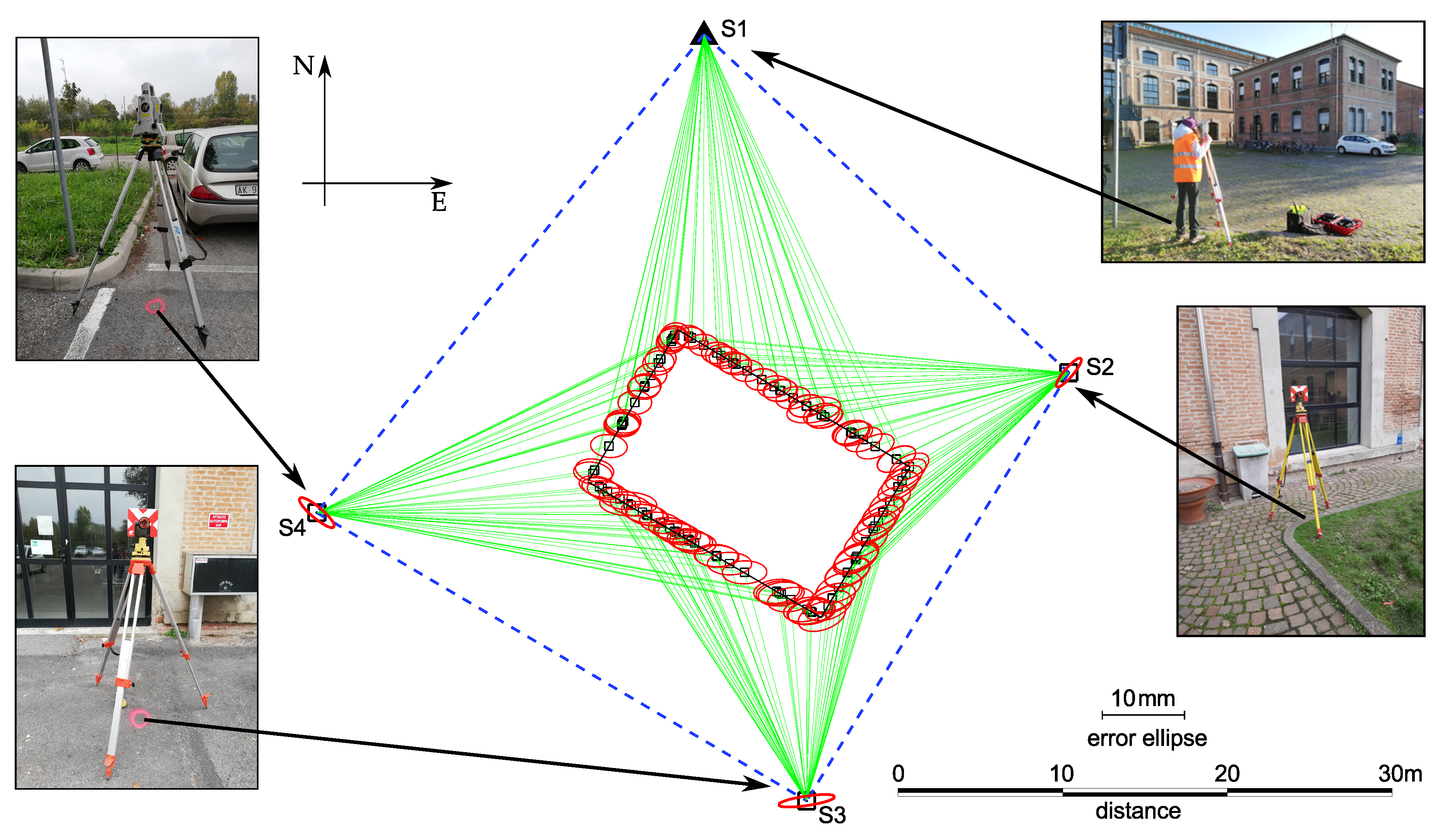
2.3.3. Network Adjustment

All of the measurements made through total station, both for benchmarks and SPs, have been adjusted using Starplus STAR*NET-PRO v.6.0.36 with a least square adjustment. In addition to total station data, we also introduced the elevation differences by leveling and the GNSS vector S1–S4. For this, the standard deviations provided by Topcon Tools have been magnified by 2 for horizontal directions and by 3 for the vertical one. The coordinates obtained for the S1 benchmark in Topcon Tools were considered as fixed during network adjustment due to the long static GNSS session on S1 of about 2 h. For total station measurements, we assumed centering errors and an uncertainty in measuring the instrument heights of 1 mm. A standard deviation of 0.2 mm was applied to elevation differences by leveling data.

The Chi square test at 5%, carried out on a total of 689 observations, of which 353 were redundant, passed with an error factor of 0.977 (lower and upper bounds were 0.926 and 1.074, respectively). Maximum semi-major axis of SP error ellipses with a confidence region of 95% was 3.5 mm, while the maximum for elevation was 1.5mm (for the same confidence level). E, N, U coordinates of each SP, as they resulted after the global adjustment, were hence assumed as “truth” for the comparison with photogrammetry results and accuracy assessment of them. In particular, the East and North coordinates were projected in UTM-zone 32 and the Up component was the ellipsoidal height in ETRS89-ETRF2000 (2008.0). Regarding elevations, we can consider the deviation of the vertical as negligible due to the very limited extent of our test-site. It is worth noting that the distance that is computed between two SPs is affected by the scale factor of the UTM projection. However, such consideration applies to the coordinates that were also obtained by photogrammetric models and, thus, the effect of the scale factor on the distance differences is negligible for our comparisons.

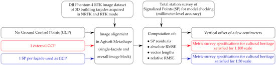
2.4. Image Dataset Acquisition

The survey of building façades was performed using the DJI-P4RTK drone. Image acquisition was planned to obtain a Ground Sample Distance (GSD) of 2 mm and with an overlap of 70% both laterally and vertically. It is worth noting that, with this GSD, each SP should have a size of $15\times 15$ pix on the acquired images and, hence, it should be easily identifiable. Furthermore, a GSD of 2 mm is required to investigate whether the survey could satisfy the requirements of a metric scale of 1:20 as reported in metric survey specifications for cultural heritage [40,41,42]. All maximum GSD that were allowed for each metric scale are reported in

Table 2. GSD and Tolerance.

Scale $1/\mathit{k}$	GSD Threshold	Absolute Tolerance	Relative Tolerance
	[m]	[m]	[m]
1:20	0.002	0.006	0.004
1:50	0.005	0.015	0.010
1:100	0.010	0.030	0.020
1:200	0.020	0.060	0.040

.

In order to perform the image acquisition, because no automatic mission was actually used due to impossibility of planning waypoint-based missions in vertical direction within the GS RTK app (at the time of our survey), we therefore signalized the ground locations in which a vertical sequence of images should have been acquired in front of each façade and at building corners (see Figure 1c and Figure 5). For obstacle-free façades (i.e., F. 1, F. 2 and F. 4), the points were signalized at 7 m from the wall and at a distance of 3 m each other, while for F. 3, the values above were reduced to 4 m and 2 m, respectively, due to the presence of the adjacent building. The resulting GSDs, as reported in Table 1, are $\approx 1.9mm$ and $\approx 1.1mm$, respectively. For each location mentioned above, we acquired a sequence of images varying the altitude of the drone, thus moving it vertically (Figure 3b). Again, for F. 1, F. 2, and F. 4, the images were captured with an altitude step of 2 m, while, for F. 3, this was reduced to 1 m. In addition, at the end of each vertical sequence (i.e., at the top of it), we also acquired some oblique images capturing from the roof up to the base of the walls. The images at building corners were captured acquiring both the visible façades entirely. The scheme of UAV image acquisition is illustrated in detail in Figure 5.

During the first session of aerial survey, we acquired the NRTK image dataset. We used the NetGEO (Topcon Positioning Italy) service for receiving NRTK corrections. Therefore, using this NRTK service the drone is automatically framed into the official Italian reference system ETRS89-ETRF2000 (2008.0). The limitation using NRTK consisted in the CORS receiver, unable to receive Galileo and BeiDou signals yet. In a further session, in a different day, we acquired the RTK dataset. The DJI D-RTK 2 Mobile Station has been placed as base receiver on S1 (Figure 3a), and then we fixed its position while using the coordinates of S1 computed through Topcon Tools. The management of the DJI D-RTK 2 Mobile Station was made with the same app used for flying: the GS RTK integrated into the remote controller of the DJI-P4RTK drone. Differently from the NRTK mode, here both base and rover receivers were able to collect GNSS data of Galileo and BeiDou in addition to GPS and GLONASS. The availability of two additional satellite constellations may have improved the fix of the integer carrier phase ambiguities near F. 3, in which there is a considerable obstacle. However, no Dilution of Precision (DOP) parameters regarding the actual distribution of satellites in the sky were saved during the performance of aerial surveys due to the kinematic mode used, neither GNSS observation files were recorded due to the limitations in manual piloting described above.

2.5. Photogrammetric Model Reconstruction and Assessment of Alignment Quality

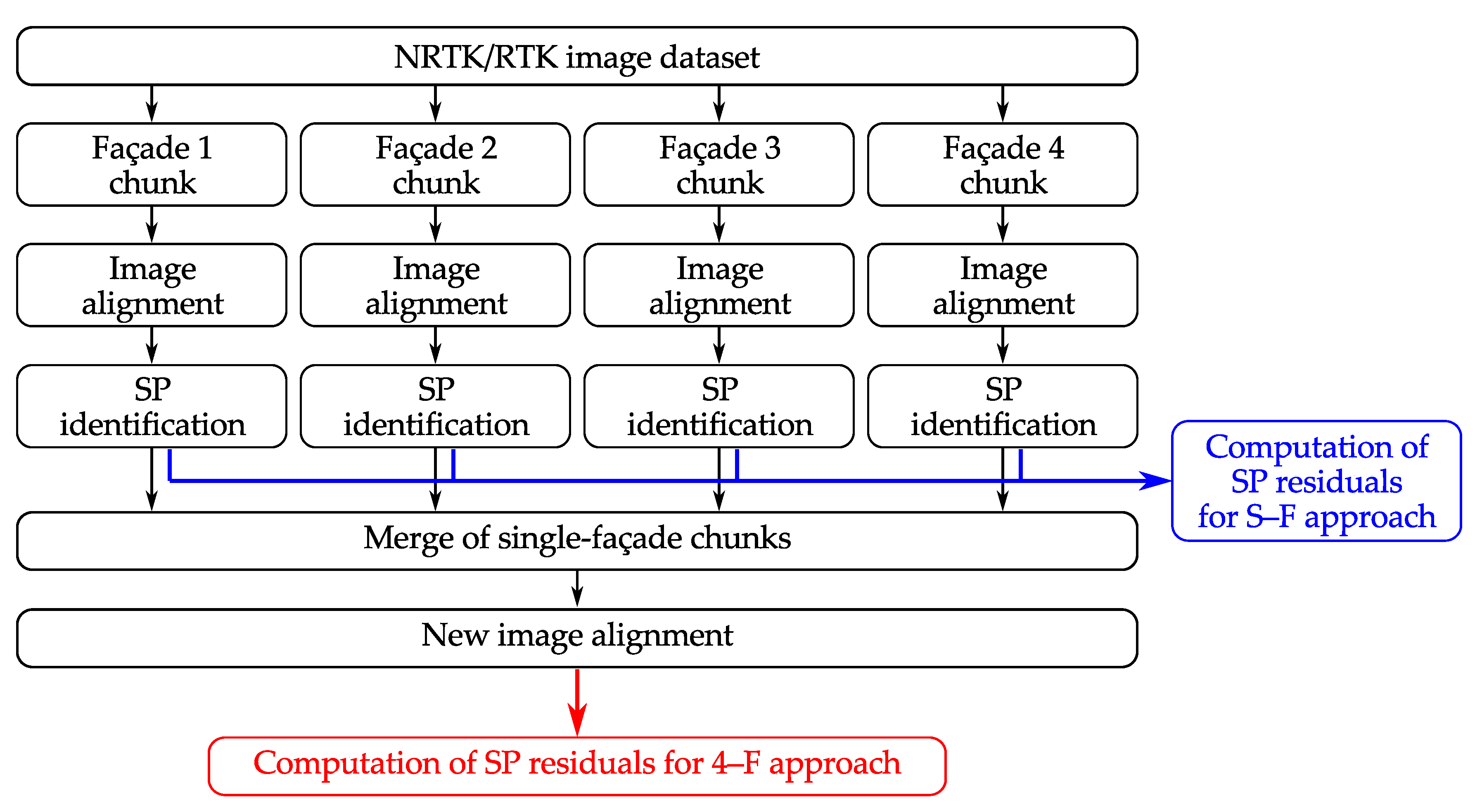
2.5.1. Generation of Photogrammetric Models

The reconstruction of building geometry through photogrammetry and Structure-from-Motion was performed while using Agisoft Metashape v.1.5. In this work, in order to testing the potential of the DJI-P4RTK + Agisoft Metashape system from the point of view of a professional user, we performed an image alignment [47,48], in which we set the accuracy parameter in Agisoft Metashape as high for all the projects and where we did not assume any limit for the overall number of tie points. During image alignment, features are automatically detected on the images by the software and tie points are consequently matched. Moreover, the camera calibration task can be performed at the same time, allowing for professional users to avoid a time-consuming pre-calibration. It is worth noting that alignments were carried out using NRTK/RTK camera locations along with the accuracy reported in Exif metadata. The assessment of the standard deviation of camera locations (as it was recorded during image acquisition and with respect to positioning accuracy of the DJI-P4RTK that is shown in Table 1) is reported in detail in Section 3.2. The remaining three exterior orientation parameters of each image (i.e., yaw, pitch, and roll) were left free to be adjusted by the software (default angular accuracy of 10°), because the IMU may be not performing enough to assume them high-accurate. Finally, we optimized all of the interior orientation parameters within the software $f,c_x,c_y,k_{1-4},b_{1-2},p_{1-4}$. In this way, the possible non-linear deformations of the model can also be removed [49]. A filtering was also performed in order to removing points with a high reprojection error or with a high level of reconstruction uncertainty; points exceeding the following thresholds (see Agisoft Metashape user manual [49] for a detailed description) were removed: reprojection error: 0.3, reconstruction uncertainty: 10, and projection accuracy: 5.

The images of each dataset (NRTK and RTK) were processed following two different strategies. For architectural purpose, indeed, a building can be described as a composition of single façades. For this reason, the first processing strategy (S–F in the following) we adopted consisted in the creation of an independent photogrammetric model for each façade. In this case, for each project, we used only the images of the considered façade and those acquired at the two corners. The number of images used in each project is reported in

Table 3. Number of images used for the creation of the photogrammetric model of façades.

Processing	Dataset
Strategy	NRTK	RTK
S–F, F. 1	59	48
S–F, F. 2	67	64
S–F, F. 3	73	66
S–F, F. 4	78	65
4–F	233	211

. The second approach (4–F in the following), in which the image datasets were processed consisted in the creation of a photogrammetric block in order to exploit the benefits of a Block Bundle Adjustment (BBA) [32]. In this way, a more robust photogrammetric reconstruction is generated and it is possible to create a single model for the entire building: tie points in common between different façades can provide additional constraints to adjust those camera locations with poorer RTK accuracy. Therefore, we also analyzed and compared the input camera locations and their accuracy with those that were obtained after the image alignment in Agisoft Metashape, for both RTK and NRTK datasets.

2.5.2. Identification of SPs on Images

We proceeded to identifying the SPs on each acquired image in order to validate the models. The intersection of rays gives an estimate of the SP positions that can be further compared to what obtained after by total station (see Section 2.3.3). It is worth noting that the repetition of SP identification through the different projects may have been a source of uncertainty making the comparison less accurate. In order to avoid this issue, the 4–F project that is described in Section 2.5.1 was created merging the four S–F chunks in Agisoft Metashape: in this way, SP projections were left unchanged and, hence, the estimate of their position depends on the alignment only. The process is summarized in Figure 6 for clarity.

Moreover, in order to assess the uncertainty introduced by the operator who identified SPs on images, we repeated the SP identification process with another operator and we computed the difference for each (i) SP, (ii) kinematic mode (NRTK and RTK), and (iii) processing strategy (S–F and 4–F).

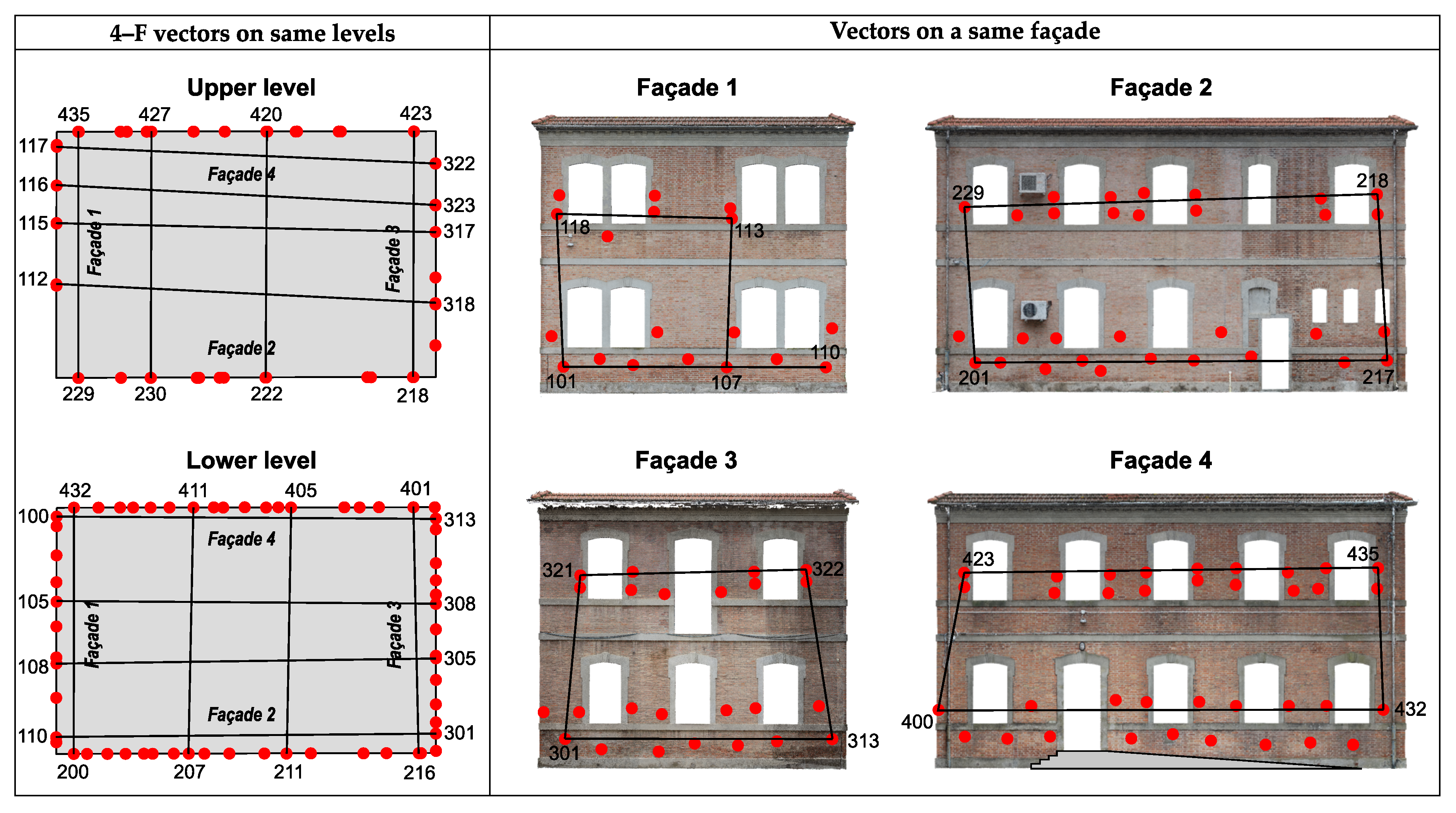
2.5.3. Computation of Residuals

The comparison between the E, N, U coordinates estimated through the photogrammetric geometry reconstruction with those surveyed by total station allowed for us to evaluate the entity and the direction of residuals for each SP. In order to do this, for each kind of processing strategy (i.e., S–F and 4–F) and for each kinematic GNSS mode used (i.e., NRTK and RTK), we computed the residuals, as follows:

$$\left\{\begin{array}{cc}\hfill \mathrm{East}\mathrm{SP}\mathrm{res}.& =E_{\mathrm{phot}}-E_{\mathrm{tot}}\mathrm{stat}\hfill \\ \hfill \mathrm{North}\mathrm{SP}\mathrm{res}.& =N_{\mathrm{phot}}-N_{\mathrm{tot}}\mathrm{stat}\hfill \\ \hfill \mathrm{Vertical}\left(\mathrm{Up}\right)\mathrm{SP}\mathrm{res}.& =U_{\mathrm{phot}}-U_{\mathrm{tot}}\mathrm{stat}\hfill \\ \hfill \mathrm{Horizontal}\mathrm{SP}\mathrm{res}.& =\sqrt{{(E_{\mathrm{phot}}-E_{\mathrm{tot}}\mathrm{stat})}^2+{(N_{\mathrm{phot}}-N_{\mathrm{tot}}\mathrm{stat})}^2}\hfill \\ \hfill 3\mathrm{D}\mathrm{SP}\mathrm{res}.& =\sqrt{{(E_{\mathrm{phot}}-E_{\mathrm{tot}}\mathrm{stat})}^2+{(N_{\mathrm{phot}}-N_{\mathrm{tot}}\mathrm{stat})}^2+{(U_{\mathrm{phot}}-U_{\mathrm{tot}}\mathrm{stat})}^2}\hfill \end{array}\right.$$

(1)

for every SP we surveyed. The computation of the residuals with Equation (1) was also carried out to proceed with the assessment of SP identification uncertainty (see Section 2.5.2).

For 3D SP residuals, we also evaluated the standard deviation combining E, N, U standard deviations, as they resulted after the network adjustment with the Root Mean Square reprojection error [39] of each SP (calculated in Agisoft Metashape over all photos in which it was visible [49]):

$$\left\{\begin{array}{cc}\hfill {\sigma }_{\mathrm{tot}\mathrm{stat}}& =\sqrt{{\sigma }_{E_{}\mathrm{tot}\mathrm{stat}}^2+{\sigma }_{N_{}\mathrm{tot}\mathrm{stat}}^2+{\sigma }_{U_{}\mathrm{tot}\mathrm{stat}}^2}\hfill \\ \hfill {\sigma }_{\mathrm{phot}}& =GSD·\left(RMS\mathrm{reprojection}\mathrm{error}\right)\hfill \\ \hfill {\sigma }_{3\mathrm{D}\mathrm{res}}& =\sqrt{{\sigma }_{\mathrm{tot}\mathrm{stat}}^2+{\sigma }_{\mathrm{phot}}^2}\hfill \end{array}\right.$$

(2)

2.5.4. Computation of Absolute and Relative RMSE

After having evaluated the residuals for each SP, we assessed the level of accuracy of the photogrammetric models computing some cultural heritage specifications: absolute and relative RMSE [40,41,42].

Absolute RMSE was computed considering the residuals (Equation (1)) in E, N, U direction for each façade, both for S–F and 4–F projects. Additionally, we computed the horizontal and 3D RMSE:

$$\mathrm{absolute}\mathrm{RMSE}{}_{\mathrm{E},\mathrm{N},\mathrm{U},\mathrm{horizontal},3\mathrm{D}}=\sqrt{{\displaystyle \frac{{\sum }_{i=1}^N{\left({\mathrm{SP}}_{\mathrm{i}}\mathrm{residual}{}_{\mathrm{E},\mathrm{N},\mathrm{U},\mathrm{horizontal},3\mathrm{D}}\right)}^2}{N}}}$$

(3)

Subsequently, we assumed a threshold value for the absolute RMSE related to the graphical scale $1/k$, as follows:

$$\mathrm{absolute}\mathrm{tolerance}=0.3mm·k$$

(4)

In this way, we evaluated which scale would have been adopted to satisfy metric survey requirements.

For the same cases above, the relative RMSE was computed while considering the vector length difference $\Delta \mathrm{L}={\mathrm{L}}_{\mathrm{phot}}-{\mathrm{L}}_{\mathrm{tot}\mathrm{stat}}$ between two SPs, instead of SP residuals:

$$\mathrm{relative}\mathrm{RMSE}=\sqrt{{\displaystyle \frac{{\sum }_{i=1}^N{\left(\Delta {\mathrm{L}}_{\mathrm{i}}\right)}^2}{N}}}$$

(5)

In order to distinguish between levels and façades (see in Section 3.4), we selected a total of 32 vectors, of which 16 with initial and final SPs belonging to a same level (i.e., 8 U.L. + 8 L.L.) and 16 with SPs on a same façade (i.e., 4 F. 1 + 4 F. 2 + 4 F. 3 + 4 F. 4).

Additionally, in this case, we assumed a threshold value for the relative RMSE related to the graphical scale $1/k$, as follows:

$$\mathrm{relative}\mathrm{tolerance}=0.2mm·k$$

(6)

Table 2 reports all of the absolute and relative RMSE tolerances for metric scales from 1:20 to 1:200.

3. Results

3.1. SP Identification Uncertainty Due to Operator

The first aspect we assessed, prior to any further consideration, consisted in evaluating which was the level of uncertainty due to operator’s discretion in identifying the SPs on the acquired images. For this, we computed the maximum and minimum difference between two different operators for each case that we analyzed.

The results are reported in

Table 4. Minimum and maximum coordinate difference due to SP identification by different operators.

Mode		S–F projects			4–F project
		E	N	U	E	N	U
NRTK	Min [m]	−0.002	−0.001	−0.003	−0.004	−0.002	−0.002
	Max [m]	0.002	0.001	0.001	0.003	0.001	0.002
RTK	Min [m]	−0.001	−0.002	−0.001	−0.004	−0.002	0.000
	Max [m]	0.002	0.002	0.001	0.003	0.002	0.002

and they highlight that the maximum difference was 4 mm. On average, the difference due to operator did not exceed a value of 2 mm and, therefore, we assumed that this aspect did not affect the comparisons in a significant way.

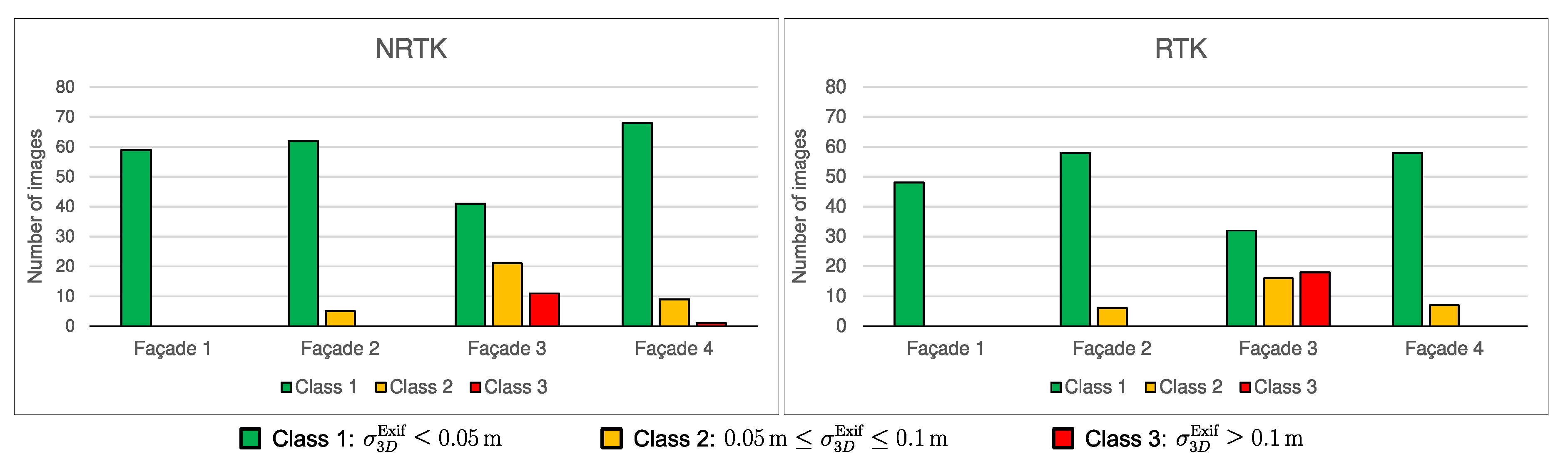
3.2. Analysis of Input Camera Locations in Agisoft Metashape

The second aspect that we assessed was the standard deviation in E, N, U directions that were assigned to camera locations during their acquisition on the basis of real-time estimated accuracy of kinematic GNSS modes. This data, available into Exif metadata, provides the theoretical accuracy with which camera locations should have been acquired. In other words, we should be able to evaluate whether the GNSS solution at the time of image capture reached a real fix of carrier phase ambiguities or not. Starting from E, N, U Exif accuracies, we computed the resulting 3D accuracy as:

$${\sigma }_{3D}^{\mathrm{Exif}}=\sqrt{{\sigma }_{E_{}\mathrm{Exif}}^2+{\sigma }_{N_{}\mathrm{Exif}}^2+{\sigma }_{U_{}\mathrm{Exif}}^2}$$

(7)

On the basis of the technical specifications of the GNSS system of DJI-P4RTK operating in kinematic mode (see Table 1), we also computed a threshold in order to classify GNSS solutions. In particular, we assumed the following threshold $T_{\mathrm{drone}}$:

$$T_{\mathrm{drone}}=3·\sqrt{{\sigma }_{H_{\mathrm{drone}}}^2+{\sigma }_{V_{\mathrm{drone}}}^2}\approx 0.05m$$

(8)

and, hence, we classified them into three classes, as follows:

$$\left\{\begin{array}{cc}{\displaystyle \frac{{\sigma }_{3D}^{\mathrm{Exif}}}{T_{\mathrm{drone}}}}<1\hfill & \mathrm{Class}1\mathrm{solution}\hfill \\ 1\le {\displaystyle \frac{{\sigma }_{3D}^{\mathrm{Exif}}}{T_{\mathrm{drone}}}}\le 2\hfill & \mathrm{Class}2\mathrm{solution}\hfill \\ {\displaystyle \frac{{\sigma }_{3D}^{\mathrm{Exif}}}{T_{\mathrm{drone}}}}>2\hfill & \mathrm{Class}3\mathrm{solution}\hfill \end{array}\right.$$

(9)

The results are shown in Figure 7, and they show that the façade closest to the adjacent building (i.e., F. 3) is the one with the highest number of class 2 and 3 images, F. 2 and F. 4 have some non-class 1 image, probably due to some locations close to the adjacent building, while F. 1 has only class 1 images (i.e., only “fixed” GNSS solutions). This is particularly interesting, because it confirms what we should expect in a condition in which the sky visual is less clear (F. 3), thus a lower rate of fix. It is worth noting that the presence of two additional satellite constellation seems not to introduce benefits looking at the standard deviation assigned to camera locations, because F. 3 in RTK mode has a higher number of class 3 solutions as compared to the NRTK mode.

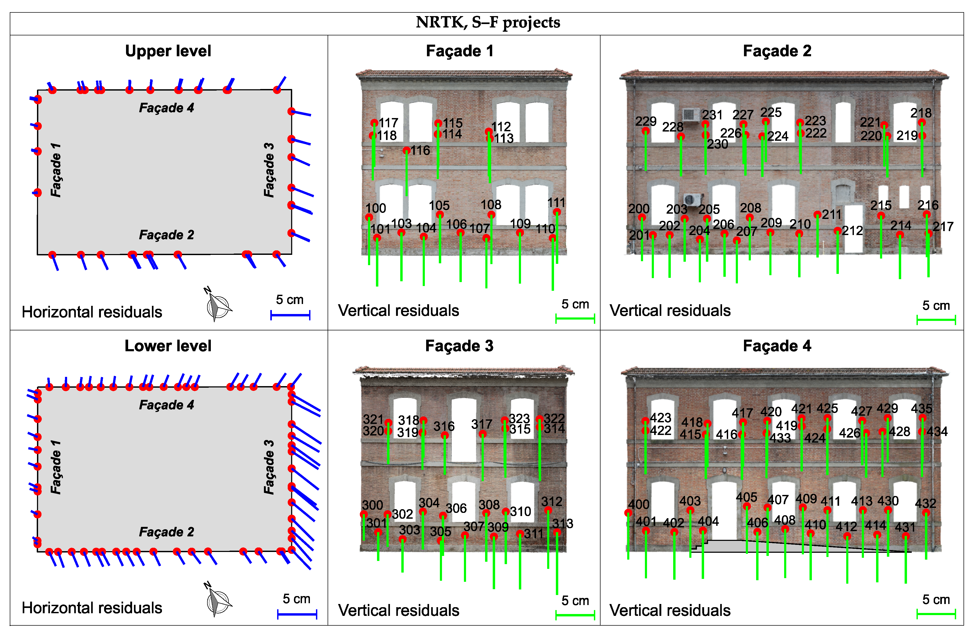
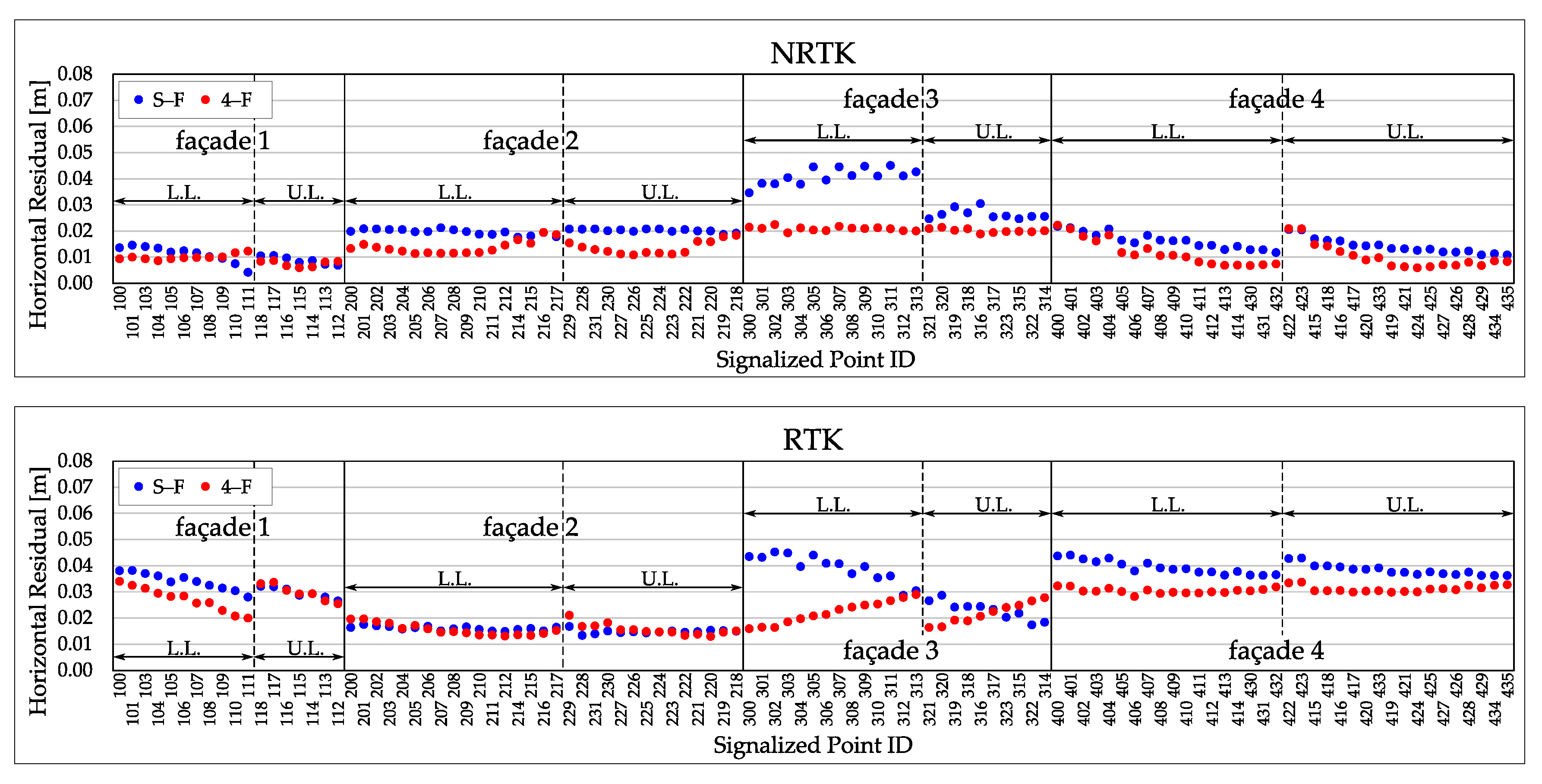
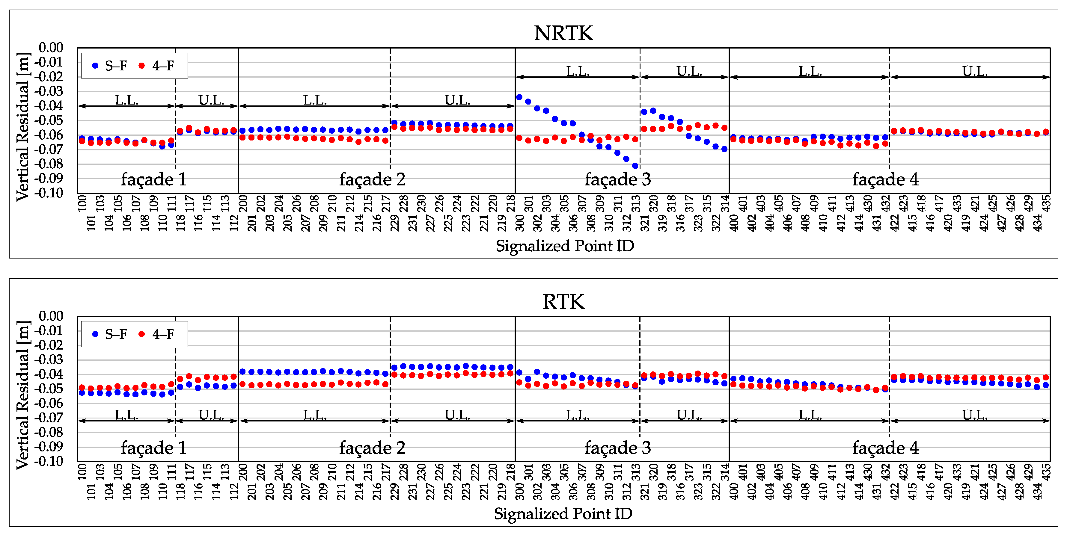
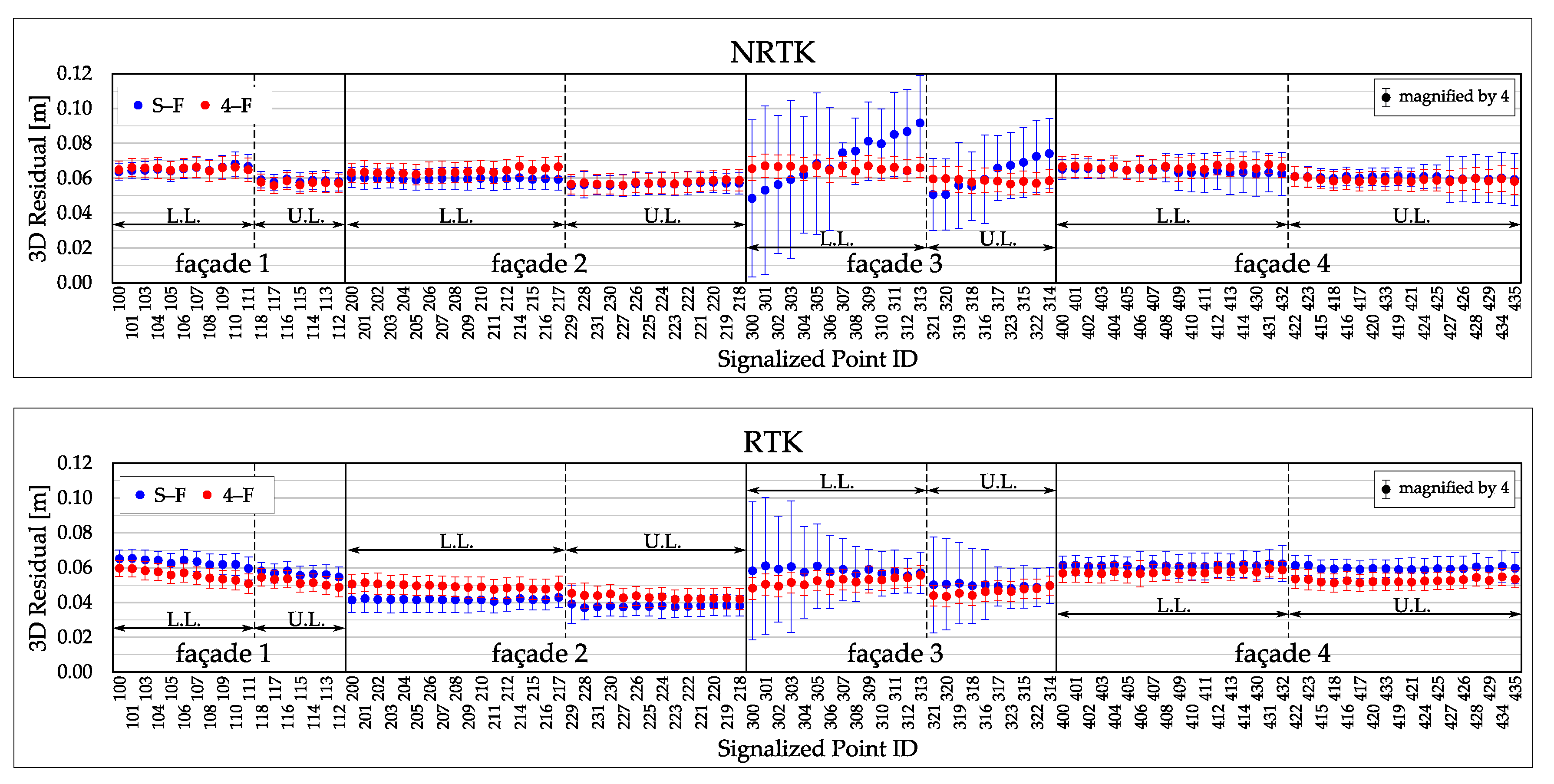
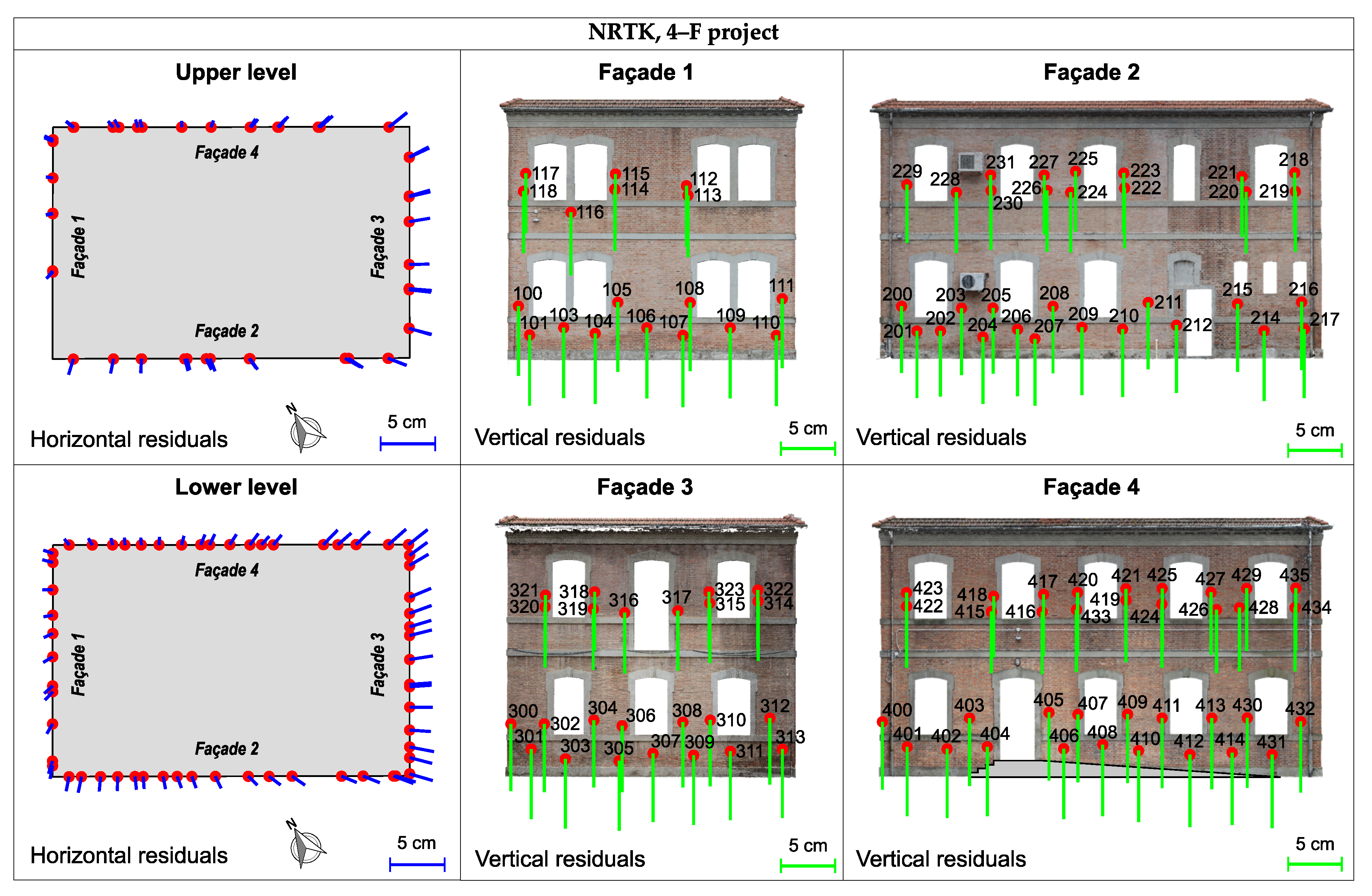
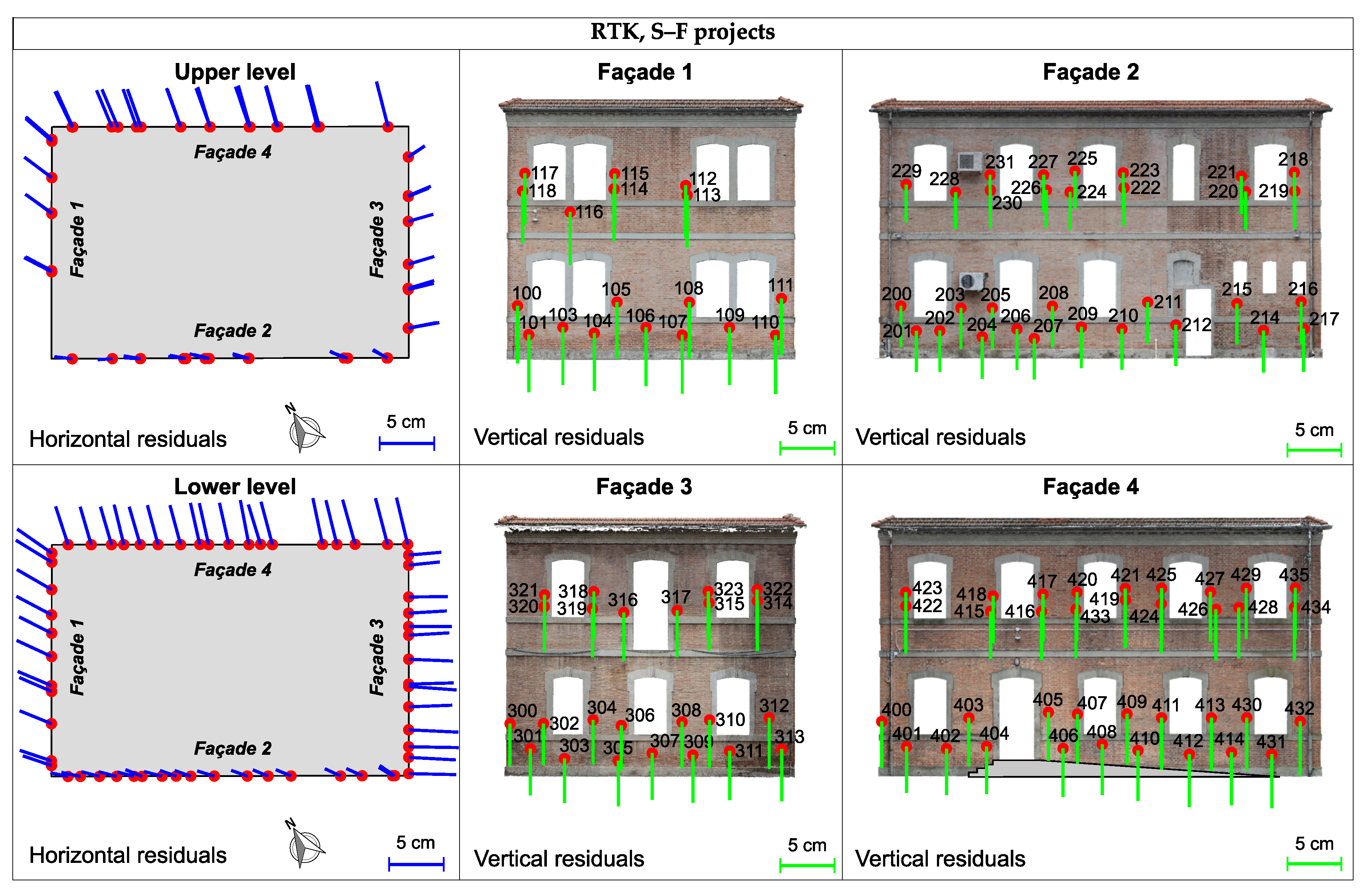
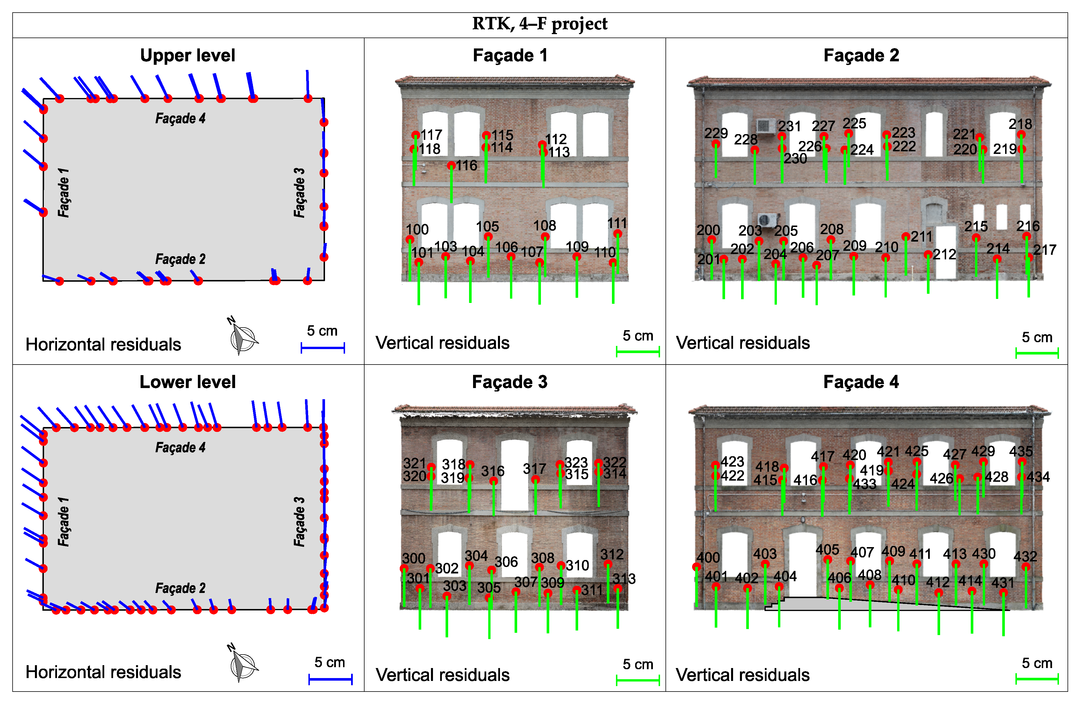
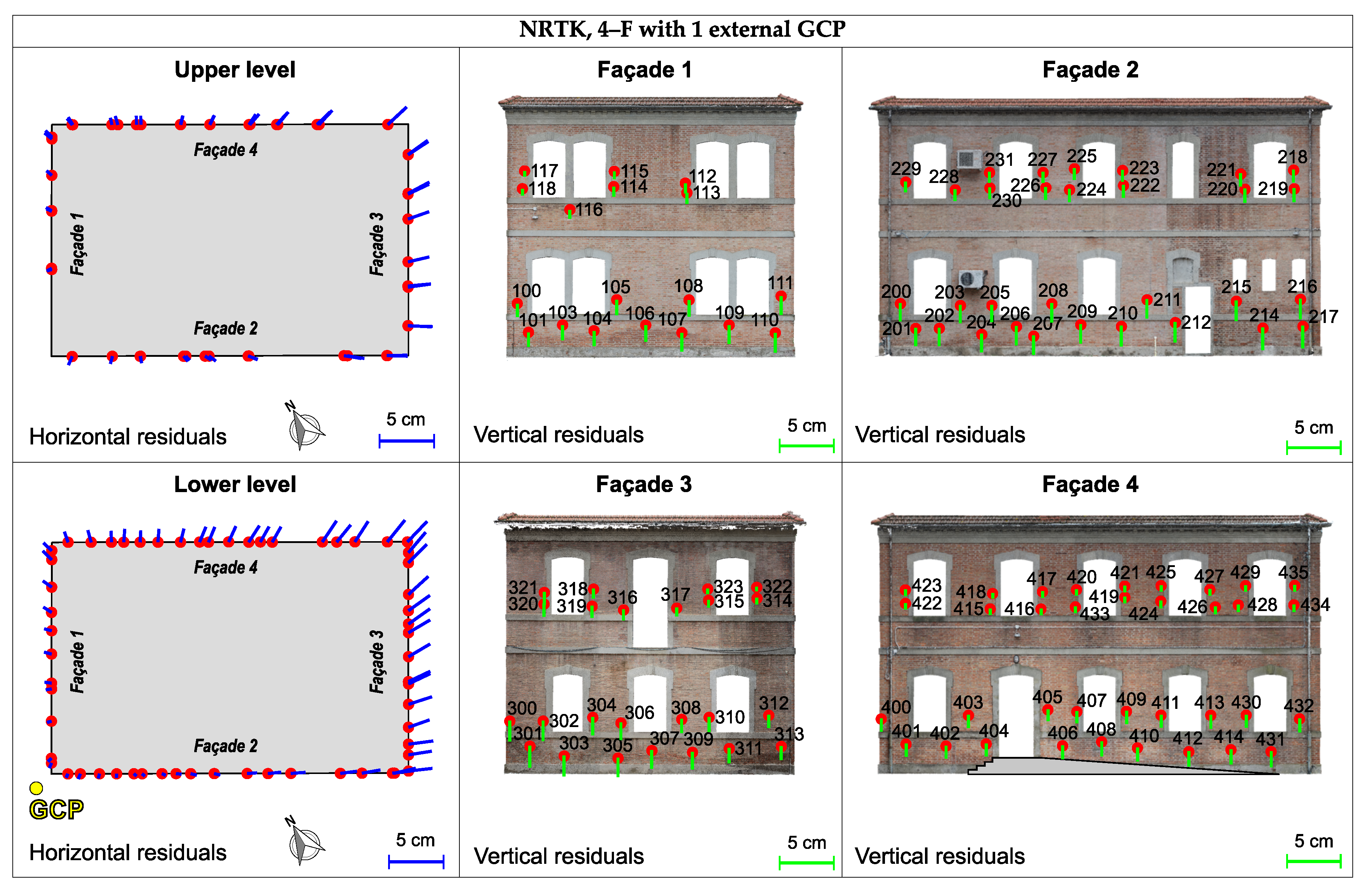
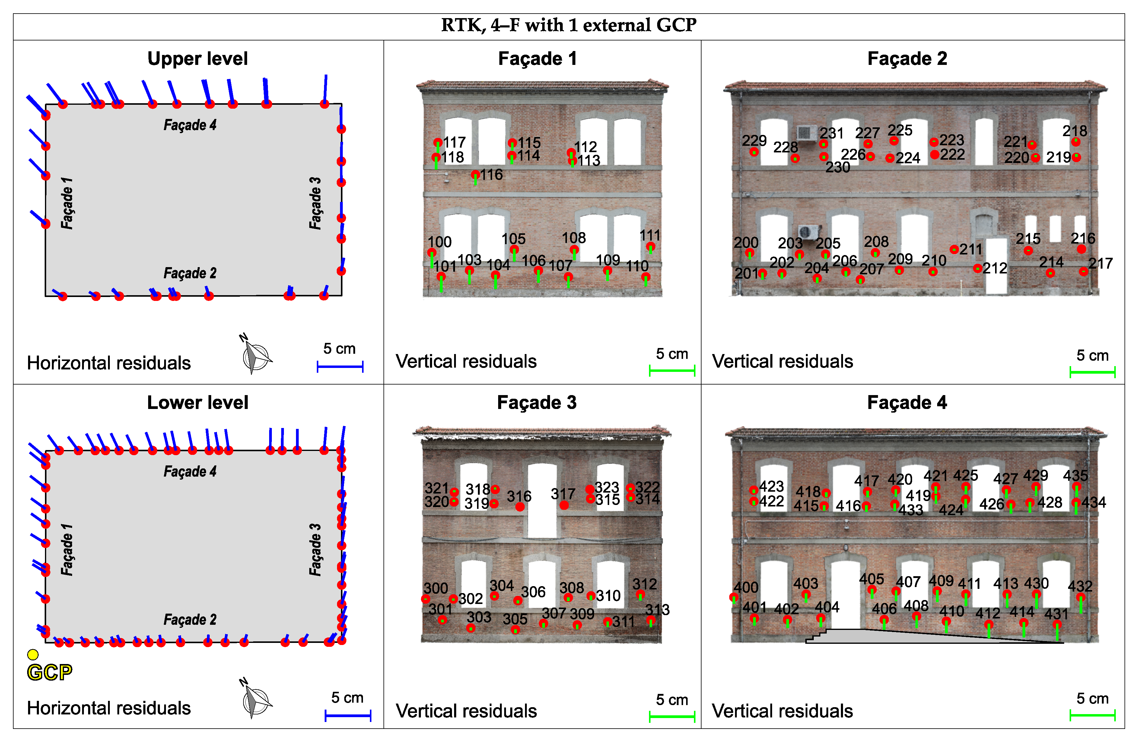
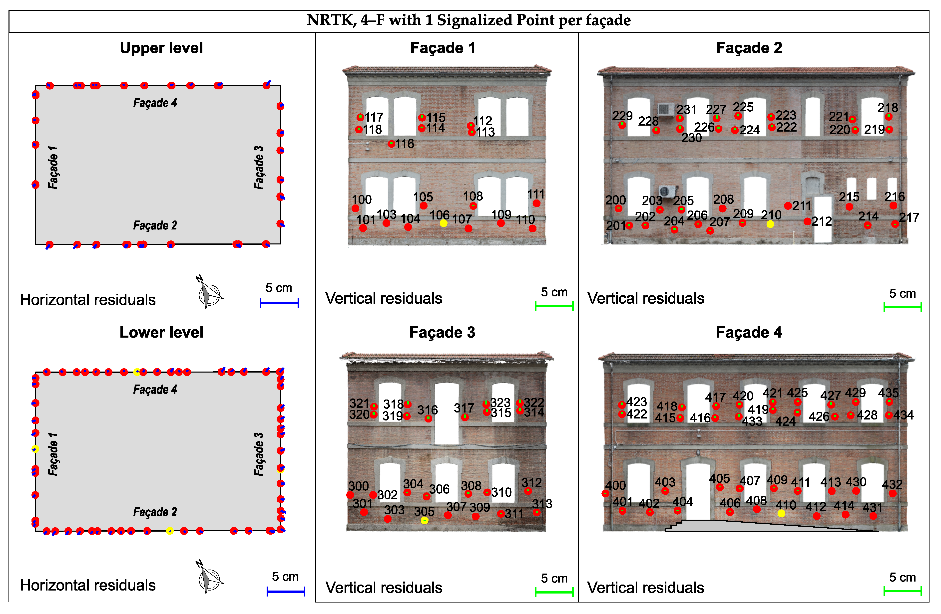
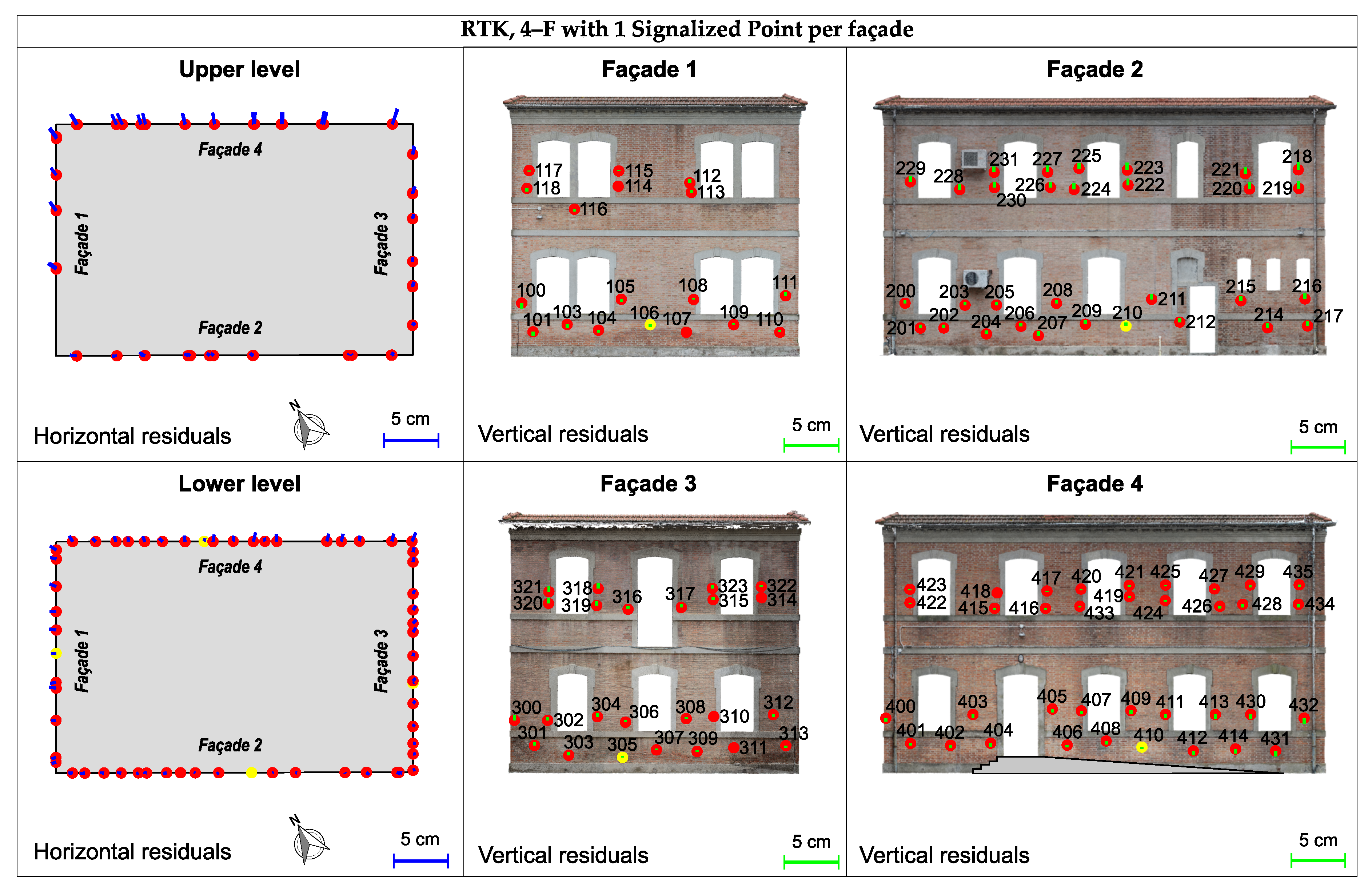
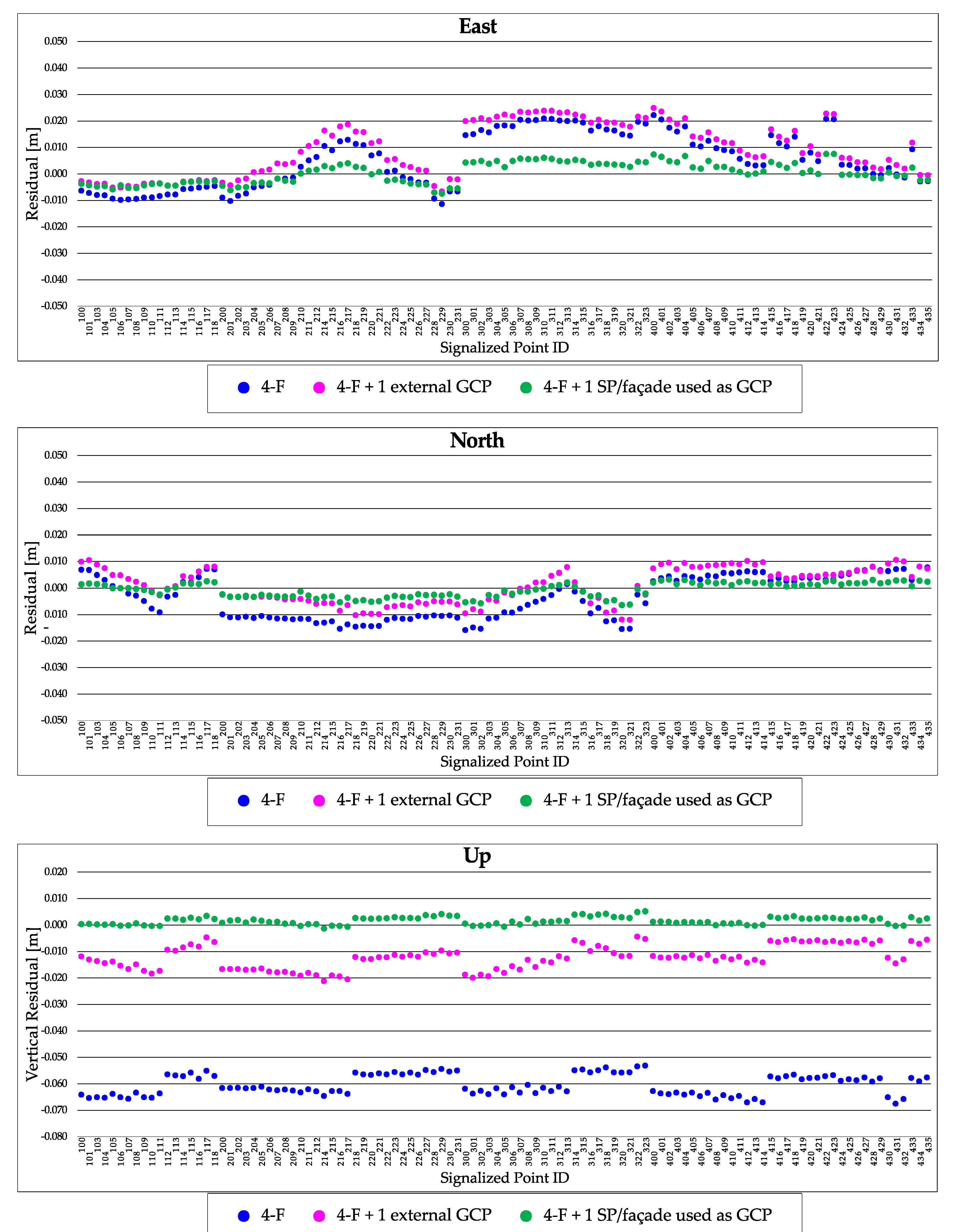
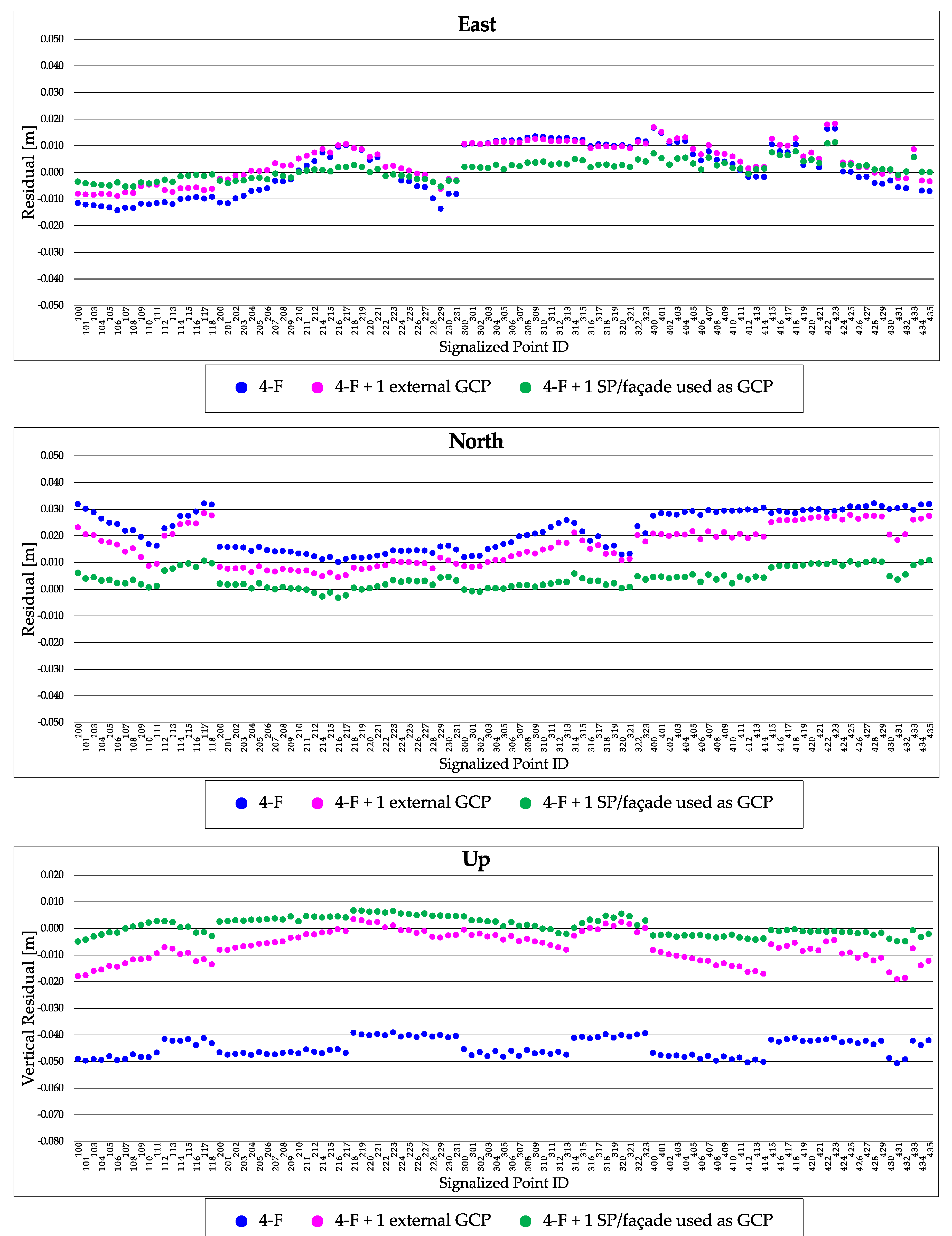
3.3. Horizontal and Vertical Residuals

We computed horizontal and vertical residuals for each image dataset (NRTK, RTK) and processing strategy (S–F, 4–F) through a self-calibration approach, as described in Section 2.5.3. The minimum, maximum, and average of such residuals are reported in

Table 5. Horizontal residuals.

Mode	Level	Project	S–F				4–F
		Façade(s)	F. 1	F. 2	F. 3	F. 4	All
NRTK	L.L.	Min [m]	0.004	0.018	0.035	0.012	0.007
		Max [m]	0.015	0.021	0.045	0.022	0.022
		Average [m]	0.011	0.020	0.041	0.016	0.014
	U.L.	Min [m]	0.007	0.019	0.025	0.011	0.006
		Max [m]	0.011	0.021	0.030	0.021	0.021
		Average [m]	0.009	0.020	0.027	0.014	0.013
RTK	L.L.	Min [m]	0.028	0.015	0.029	0.036	0.013
		Max [m]	0.038	0.018	0.045	0.044	0.034
		Average [m]	0.034	0.016	0.039	0.039	0.024
	U.L.	Min [m]	0.027	0.013	0.017	0.036	0.013
		Max [m]	0.032	0.017	0.029	0.043	0.034
		Average [m]	0.030	0.015	0.023	0.038	0.025

and

Table 6. Vertical residuals.

Mode	Level	Project	S–F				4–F
		Façade(s)	F. 1	F. 2	F. 3	F. 4	All
NRTK	L.L.	Min [m]	−0.068	−0.058	−0.081	−0.064	−0.068
		Max [m]	−0.062	−0.056	−0.034	−0.061	−0.060
		Average [m]	−0.064	−0.056	−0.057	−0.062	−0.064
	U.L.	Min [m]	−0.059	−0.054	−0.070	−0.060	−0.059
		Max [m]	−0.057	−0.052	−0.043	−0.057	−0.053
		Average [m]	−0.058	−0.053	−0.056	−0.059	−0.056
RTK	L.L.	Min [m]	−0.054	−0.040	−0.048	−0.050	−0.051
		Max [m]	−0.052	−0.038	−0.038	−0.043	−0.045
		Average [m]	−0.053	−0.038	−0.043	−0.047	−0.048
	U.L.	Min [m]	−0.049	−0.035	−0.046	−0.049	−0.044
		Max [m]	−0.047	−0.034	−0.042	−0.044	−0.039
		Average [m]	−0.048	−0.035	−0.044	−0.046	−0.041

for each level of the building (L.L. and U.L.). The direction and magnitude of the residuals are also illustrated in Figure 8 and in Appendix A from Figure A1 to Figure A3. As regards NRTK dataset, the maximum horizontal residual is 0.022 m for obstacle-free façades and 0.045 m for F. 3. The former value is comparable with the accuracy of NRTK positioning, while the latter is certainly conditioned by the presence of the adjacent building. However, it is also worth noting that the overall bundle adjustment around the entire building, as well as the more constraints that are introduced by obstacle-free façades, made the maximum residual to be 0.022 m also including F. 3. Using RTK dataset, the F. 3 project is still characterized by a maximum horizontal residual of 0.045 m and, unexpectedly, also F. 4 shows a maximum residual of 0.044 m, even if it is an obstacle-free façade. The 4–F project highlighted a maximum horizontal difference of 0.034 m that is generally lower than those of RTK S–F project, but it higher than the corresponding value we obtained for the NRTK dataset mentioned above.

From a vertical point of view, SP residuals of NRTK dataset show a maximum negative difference of 0.081 m for F. 3 and 0.068 m for obstacle-free façades. The latter value is also the maximum elevation residual for the 4–F project. Conversely, the residuals for the RTK dataset highlight a different situation, in which F. 1 (that is obstacle-free) has a maximum negative elevation difference of 0.054 m that is higher than the maximum evaluated on F. 3 (0.048 m). In this case, the 4–F project is characterized by a maximum vertical residual (0.044 m) that is comprised between the previous S–F values. It is interesting to highlight that all of the vertical residuals were found to be negative and they seem to be biased by a quantity of a few centimeters.

Additionally, we can note that 4–F projects are characterized by residuals that are generally lower as compared to the corresponding ones of S–F projects, due to the BBA performed on an object (i.e., our test-site building) with a closed shape, like a sort of ring. Moreover, the direction of horizontal residuals appears radial with respect to the building center (in particular for NRTK dataset), while S–F projects show horizontal residuals that seem to be biased of a quantity that is almost constant for each S–F model (see Figure 8 and Figure A1). The offset, however, is different from project to project. A mean value of such bias is also reported in Table 5. The 4–F project in RTK mode highlights; instead, a singular behavior in correspondence of F. 3, as compared to the S–F project in RTK mode, in which the horizontal residuals become parallel to the façade with a rotation of about 90° (see Figure A2 and Figure A3). Regarding the vertical direction, both NRTK and RTK residuals present an offset that leads to underestimating the elevation, from −0.034 m up to −0.081 m. On average, the bias evaluated across all S–F and 4–F projects for both the NRTK and RTK image datasets ranged from −0.037 m (RTK, S–F, F. 2) to −0.060 m (NRTK, S–F, F. 1).

Horizontal and vertical residuals are also illustrated in Figure 9 and Figure 10, in which they are divided for single façades per level and in sequence from the left to the right looking at each façade frontally (see SP ID on the x-axis). The analysis of the graphs highlights that horizontal residuals generally assume a maximum value of about 2 cm for NRTK dataset, except for F. 3. Indeed, for this façade, the residuals are clearly higher for the S–F model, in particular in the lower level in which the obstruction effect of the adjacent building is more impacting. An improvement is evident when processing all the façades together (4–F), since the horizontal residuals decrease to a value of ≈2 cm, once again. For RTK dataset, similar considerations can be applied, even if the horizontal residuals tend to remain slightly higher than those mentioned above, also in the 4–F project (≈3 cm). Regarding vertical residuals, we can note that lower values are generally found for the upper level of SPs. This fact can be due to the introduction of oblique images that are captured at the top of each vertical acquisition path as well as a higher accuracy of camera locations with a clearer visual of the sky with more satellites available for computing kinematic GNSS solutions.

It is interesting noting that F. 3 has a singular behavior with a S–F approach performed while using the NRTK dataset. In this case, in fact, the vertical residual varies with continuity from edge to edge and the difference is about 4.5 cm for the lower level and 3 cm for the upper one. This effect is dampened with a 4–F approach: the maximum vertical residual is $\approx 3cm$ and the range decreases to $\approx 1.5cm$. Finally, the analysis of 3D residuals (see Figure 11) shows, once again, how most of the error is due to the Up component that is probably affected by some kind of bias and that the creation of a single model allows for one to considerably reduce the magnitude of the residuals of F. 3, in particular for our NRTK dataset. Figure 11 also reports the standard deviation computed with Equation (2) of Section 2.5.3.

Moreover, it is also worth noting that the highest standard deviation and, thus, the lowest accuracy, is found for the S–F model of F. 3 for both NRTK and RTK datasets. This depends on the higher reprojection error of SPs that has been used to estimate the accuracy of the photogrammetry-based position of SPs. Additionally, this is due to the effect of the adjacent building that obstructs the sky visual and causes GNSS solutions of camera locations to be less accurate, from which it is derived that the photogrammetric block of a the S–F project of F. 3 is less robust. The highest standard deviation was 1.2 cm and, indeed, it has been found for the point 301 that is located close to the ground and, hence, in a critical position for obtaining a GNSS fix. Conversely, the same point shows a standard deviation of only 2 mm in the 4–F project, which is also the maximum value that we found for all the SP standard deviations of 4–F project.

3.4. Computation of Absolute and Relative RMSE

We computed absolute RMSE to assess the accuracy of the photogrammetric reconstructions with respect to the building truth consisting of the final surveyed coordinates of the SPs, as described in Section 2.5.4. The absolute RMSE for each E, N, U direction, along with the horizontal (2D) and 3D RMSE, for all of the projects with self-calibration and the use of camera locations only (i.e., no SP or GCP ever used) is shown in

Table 7. Absolute Root Mean Square Errors (RMSE)–NRTK dataset. The scale whose metric survey specifications were satisfied is also reported in brackets.

Mode	Façade	Absolute RMSE [m] (Scale)
		E	N	U	Horizontal	3D
S–F	F. 1	0.007	0.008	0.062	0.011 (1:50)	0.063 (<1:200)
	F. 2	0.002	0.020	0.055	0.020 (1:100)	0.058 (1:200)
	F. 3	0.017	0.032	0.058	0.036 (1:200)	0.068 (<1:200)
	F. 4	0.012	0.010	0.060	0.016 (1:100)	0.062 (<1:200)
4–F	All	0.012	0.009	0.061	0.015 (1:50)	0.062 (<1:200)

for NRTK dataset and

Table 8. Absolute RMSE–RTK dataset. The scale whose metric survey specifications were satisfied is also reported in brackets.

Mode	Façade	Absolute RMSE [m] (Scale)
		E	N	U	Horizontal	3D
S–F	F. 1	0.016	0.028	0.028	0.033 (1:200)	0.061 (<1:200)
	F. 2	0.010	0.012	0.037	0.016 (1:100)	0.040 (1:200)
	F. 3	0.030	0.016	0.043	0.034 (1:200)	0.055 (1:200)
	F. 4	0.010	0.038	0.046	0.039 (1:100)	0.060 (<1:200)
4–F	All	0.009	0.023	0.045	0.025 (1:100)	0.051 (1:200)

for the RTK one. Additionally, we reported the scale whose requirements were satisfied by the final model accuracy. It is worth noting that, horizontally, the NRTK dataset proved to satisfy the requirements of a metric survey for a scale of 1:100 (with the only exception of F. 3, due to the higher uncertainty of GNSS solution of camera locations, which was likely caused by the multipath effect) with a S–F approach. Similarly, the 4–F project was found to produce an horizontal metric survey that is suitable for a scale of 1:50. The RTK dataset exhibited a slightly lower level of accuracy that never satisfied the requirements of 1:50. In 3D, the presence of a bias is evident in all cases and it affected the computation of the absolute RMSE causing final results that, for the RTK dataset, are suitable for the lower scale we took into account in this work (i.e., 1:200).

For such reasons, in order to fix the vertical offset issue between the 4–F projects and the SPs, we investigated (i) the introduction of a GCP external to the building (abbreviated as 4–F + 1 ext GCP in the following) as well as (ii) the use of one SP per façade as GCP (abbreviated as 4–F + 1 SP/façade in the following). The external GCP was not signalized during image dataset acquisition, because we noticed the vertical offset of models only after image alignments. Subsequently, we decided to assume a natural point afterwards that was also easily and clearly identifiable on the images already acquired. This GCP, located on the external sidewalk of the building (at the corner between F. 1 and F. 2, see Figure 5) was surveyed in static GNSS mode and its elevation was assumed with an accuracy of 4 mm in Agisoft Metashape. Elevation was also verified through a leveling and the assumed precision was successfully confirmed. We decided to survey the external GCP using a GNSS receiver, since this is less time-consuming with total station. In particular, we used static GNSS instead of NRTK/RTK due to the closeness of our test-site building. For option (ii), the SP used as a GCP was selected in the center of each façade in order to be visible in the highest number of acquired images as possible (SP ID: 106 on F. 1, 210 on F. 2, 305 on F. 3, 410 on F. 4 (see Figure 8)).

In addition, camera location accuracy was modified, magnifying the horizontal standard deviations of a factor of 2 and the vertical one of a factor of 5. This aimed to “unlock” camera locations, enhancing the effect of introducing GCPs. The results, as reported in

Table 9. Absolute RMSE for different bias-fixing strategies. The scale whose metric survey specifications were satisfied is also reported in brackets.

Mode	Type	Absolute RMSE [m] (Scale)
		4–F	4–F + 1 ext GCP	4–F + 1 SP ${}^{†}$/façade
NRTK	Horizontal	0.015 (*)	0.015	0.005
		(1:50)	(1:50)	(1:50)
	3D	0.062 (*)	0.020	0.005
		($<1:200$)	(1:100)	(1:50)
RTK	Horizontal	0.025 (**)	0.020	0.006
		(1:100)	(1:100)	(1:50)
	3D	0.051 (**)	0.022	0.007
		(1:200)	(1:100)	(1:50)

${}^{†}$ used as GCP, * value reported in Table 7, ** value reported in Table 8.

, show such an improvement in both horizontal and 3D accuracies, also allowing for one to satisfy the requirements of a greater scale of detail. In addition, the graphs of all the vertical SP residuals are shown in Appendix B (Figure A8 and Figure A9). Horizontal and vertical residuals (discussed in Section 3.3 for the cases with the use of NRTK/RTK camera locations only) are also reported for these further projects in Appendix A (Figure A4–Figure A7).

In order to evaluate the deformation of the models, we also computed the relative RMSE selecting 16 horizontal vectors between SPs on opposite façades, for each level of the building and 16 for each couple of façades (i.e, 1-3 and 2-4), and we computed their own deformation as a vector length difference $\Delta \mathrm{L}={\mathrm{L}}_{\mathrm{phot}}-{\mathrm{L}}_{\mathrm{tot}\mathrm{stat}}$. Vectors that were assumed for this purpose are illustrated in Figure 12, while the length differences are reported in

Table 10. Quality assessment of the 4–F models through vectors between SPs located on opposite façades and on a same level (vectors are illustrated in Figure 12 on the left side). Relative RMSE together with the scale whose metric survey specifications were satisfied are also reported.

Level	Vector	$L_{\mathbf{tot}\mathbf{stat}}$ [m]	$L_{\mathbf{phot}}$ [m]		$\Delta L$ [m]
			NRTK	RTK	NRTK	RTK
L.L.	100–313	16.395	16.420	16.419	0.025	0.024
	105–308	16.373	16.402	16.398	0.029	0.025
	108–305	16.448	16.475	16.473	0.027	0.025
	110–301	16.391	16.415	16.413	0.024	0.022
	200–432	10.628	10.647	10.644	0.019	0.016
	207–411	10.717	10.735	10.732	0.018	0.015
	211–405	10.624	10.641	10.640	0.017	0.016
	216–401	10.661	10.682	10.680	0.021	0.019
U.L.	112–318	16.378	16.404	16.400	0.026	0.022
	115–317	16.373	16.398	16.394	0.025	0.021
	116–323	16.432	16.457	16.454	0.026	0.022
	117–322	16.364	16.389	16.387	0.026	0.023
	218–423	10.603	10.623	10.621	0.020	0.019
	222–420	10.627	10.645	10.645	0.017	0.017
	230–427	10.639	10.658	10.655	0.019	0.016
	229–435	10.644	10.664	10.661	0.020	0.017
			Relative RMSE [m]		0.023	0.020
			Scale		1:200	1:100

and

Table 11. Quality assessment of the S–F and 4–F models through vectors between SPs located on a same façade (vectors are illustrated in Figure 12 on the right side). Relative RMSE together with the scale whose metric survey specifications were satisfied are also reported.

Façade	Vector	$L_{\mathbf{tot}\mathbf{stat}}$ [m]	$L_{\mathbf{phot}}$ [m]				$\Delta L$ [m]
			NRTK		RTK		NRTK		RTK
			S–F	4–F	S–F	4–F	S–F	4–F	S–F	4–F
F. 1	101–110	$9.110$	$9.111$	$9.124$	$9.120$	$9.122$	$+0.001$	$+0.013$	$+0.010$	$+0.011$
	118–113	$6.074$	$6.076$	$6.084$	$6.082$	$6.082$	$+0.002$	$+0.010$	$+0.008$	$+0.008$
	101–118	$5.305$	$5.309$	$5.313$	$5.309$	$5.311$	$+0.004$	$+0.008$	$+0.004$	$+0.007$
	107–113	$5.167$	$5.175$	$5.176$	$5.172$	$5.174$	$+0.007$	$+0.009$	$+0.005$	$+0.007$
F. 2	201–217	$14.414$	$14.417$	$14.435$	$14.417$	$14.435$	$+0.003$	$+0.021$	$+0.003$	$+0.021$
	218–229	$14.446$	$14.450$	$14.468$	$14.450$	$14.467$	$+0.004$	$+0.022$	$+0.004$	$+0.022$
	201–229	$5.458$	$5.463$	$5.465$	$5.461$	$5.465$	$+0.005$	$+0.007$	$+0.003$	$+0.007$
	217–218	$5.826$	$5.829$	$5.835$	$5.831$	$5.834$	$+0.003$	$+0.008$	$+0.005$	$+0.008$
F. 3	301–313	$9.277$	$9.284$	$9.293$	$9.282$	$9.289$	$+0.007$	$+0.017$	$+0.005$	$+0.013$
	321–322	$7.841$	$7.845$	$7.855$	$7.846$	$7.852$	$+0.004$	$+0.014$	$+0.004$	$+0.010$
	301–321	$5.701$	$5.695$	$5.709$	$5.702$	$5.708$	$-0.005$	$+0.008$	$+0.001$	$+0.007$
	313–322	$5.942$	$5.952$	$5.952$	$5.944$	$5.950$	$+0.011$	$+0.010$	$+0.002$	$+0.008$
F. 4	400–432	$15.573$	$15.588$	$15.596$	$15.574$	$15.594$	$+0.015$	$+0.023$	$+0.001$	$+0.021$
	423–435	$14.494$	$14.510$	$14.516$	$14.499$	$14.515$	$+0.016$	$+0.022$	$+0.005$	$+0.022$
	400–423	$4.886$	$4.891$	$4.892$	$4.885$	$4.892$	$+0.005$	$+0.006$	$-0.001$	$+0.006$
	432–435	$4.966$	$4.969$	$4.975$	$4.969$	$4.973$	$+0.003$	$+0.008$	$+0.003$	$+0.007$
			Relative RMSE [m]				0.007	0.014	0.005	0.013
			Scale				1:50	1:100	1:50	1:100

. The relative RMSE, as compared with the thresholds reported in Table 2, shows a final metric survey level that is not suitable for a scale of 1:50 horizontally. However, the situation with respect to absolute terms improved as regards on-façade vectors. In fact, NRTK and RTK both exhibit the same behavior satisfying 1:100 requirements for 4–F projects and 1:50 for S–F ones.

Once again, we investigated the improvements introduced by the addition of an external GCP or one SP per façade (used as GCP) in image alignment and model creation also in relative terms. The results, as reported in

Table 12. Relative RMSE for different bias-fixing strategies. The scale whose metric survey specifications were satisfied is also reported in brackets.

Mode	Type	Relative RMSE [m] (Scale)
		S–F	4–F	4–F + 1 ext GCP	4–F + 1 SP ${}^{†}$/façade
NRTK	Same level	–	0.023 (*)	0.020	0.008
		–	(1:200)	(1:100)	(1:50)
	Same façade	0.007 (**)	0.014 (**)	0.013	0.005
		(1:50)	(1:100)	(1:100)	(1:50)
RTK	Same level	–	0.020 (*)	0.017	0.008
		–	(1:100)	(1:100)	(1:50)
	Same façade	0.005 (**)	0.013 (**)	0.010	0.005
		(1:50)	(1:100)	(1:100)	(1:50)

${}^{†}$ used as GCP, * value reported in Table 10, ** value reported in Table 11

, highlight that the simple introduction of an external GCP and the assumption of a lower camera location accuracy produces a model that satisfies the requirements of a scale of 1:100, whereas the use of a single SP per façade as a GCP improved the final model accuracy to the standards of 1:50.

4. Discussion

In this work, we carried out an accuracy assessment test for evaluating the potential in using the DJI-P4RTK drone for the surveying and modeling of a building in an easy, but very accurate, way. The aim was to investigate the potential of the DJI-P4RTK with particular regard to professional users.

In general, the acquisition of image datasets for the reconstruction of the geometry and shape of 3D objects requires the execution of flight plan, where the drone should follow a vertical path to acquire frontal images of the façades. Unfortunately, we were not able to actually perform any automatic mission due to the impossibility of performing a flight plan in which the altitude of the aircraft above the ground level could be varied on the vertical (e.g., introducing waypoints) and we consequently had to manually fly the drone. Furthermore, in manual mode, no RINEX file of GNSS observations was ever recorded by the drone to testing also a PPK approach. However, the acquisition of two different datasets in NRTK and RTK mode allowed for us to evaluate the possible differences between real-time kinematic GNSS approaches. According to what is generally required for generating architectural drawings of a building, we generated photogrammetric models both processing the image datasets for single façades (S–F) and through the creation of an overall block (4–F). Finally, we computed the residual for each SP whose coordinates were surveyed with total station and analyzed variations.

Prior to doing that, it is worth noting that SP identification by different operators proved to be a negligible aspect for the final comparison of results, with a maximum repeatability error of 4 mm ($\approx 2\mathrm{GSD}$). The multipath effect on computing real-time GNSS solutions in F. 3 conditions can explain such a difference, since the camera locations were less accurate, as we investigated in Section 3.2. A summary of materials and methods along with the main results of this research is reported in Figure 13 for clarity.

The analysis of SP residuals without the introduction of any GCP for the georeferencing of the model, with a self-calibration approach, showed a maximum horizontal error slightly higher than 2 cm in NRTK and 3 cm in RTK mode for the case of the entire block processing. Such values are compatible with the use of an on-board multi-frequency multi-constellation GNSS receiver in NRTK/RTK mode. The constraints that are provided by the tie points (automatically matched by Agisoft Metashape) in common between the obstacle-free façades and F. 3 can overcome to the poor accuracy of exterior orientation parameters of the images of F. 3 itself.

The discussion of vertical residuals requires a dedicated consideration. In fact, apart from a quite singular behavior of vertical residuals for the S–F of F. 3 in NRTK mode (see Figure 10), the presence of an offset between the photogrammetric models and the elevation of the SPs seems to be evident and clearly noticeable. The bias was present in both NRTK and RTK datasets. It is worth noting that (i) SP elevations derived from a rigorous process of network adjustment with a final accuracy of a few millimeters and (ii) the elevation of S1 benchmark has been verified through the post-processing of two different and independent static GNSS sessions. Furthermore, (iii) the RTK mode with base and rover receivers should ensure a centimeter-level accuracy with “random” and substantially unbiased vertical errors, even when the assumed elevation of the base slightly differs from its real value, whereas in NRTK mode the antenna phase center of the drone is directly framed into the same reference system (and frame) of the network service used for receiving corrections. Therefore, we believe that the reason of the vertical offset found in this work should be due to other aspects not related to the survey and setup of our test. Moreover, Kalacska et al. [38] found a vertical offset in models that were generated through the use of nadiral datasets of DJI-P4RTK and explored the possibility to removing it by manually modifying the focal length of the camera. In our work, the geometry and scheme acquisition is different from simply having images acquired with the optical axis normal to the object surface (that is the situation of nadiral images of the landscape) and, thus, we did not follow the same approach.

However, the computation of absolute RMSE with regard to metric survey specifications [40] is affected by the vertical bias that we found in our models and, therefore, we were interested in finding a quick method for eliminating it. The simplest approaches consisted in (i) introducing a GCP surveyed through GNSS on the external sidewalk or (ii) using one SP per façade as GCP. Subsequently, we proceeded to create new models, also assuming a lower accuracy of input camera location (especially for what concerning the vertical direction) and assessing SP residuals again. The option (i) proved to allow one to considerably reduce the vertical bias, still maintaining the same error level in horizontal directions. The best results were achieved with option (ii), where the maximum residuals evaluated on the SPs not used as GCP turned out to be $\approx 1\mathrm{cm}$ in all E, N, U directions, as also expected on the basis of usual image data processing and photogrammetric model reconstruction with non-RTK camera locations.

In relative terms, we also computed a relative RMSE assessing the deformation of vectors that were selected across opposite façades and on a same façade. As concerns vectors that were located on a single façade, the S–F strategy without the use of any GCP proved to produce results that were suitable for a metric scale of 1:50. However, with a 4–F strategy, it was only by using the option (ii) mentioned above that it was possible to obtain the same level of accuracy, both for horizontal and on-façade vectors.

The results of this research show how the DJI-P4RTK represents a powerful tool useful for the survey of buildings in an architectural context by professional users. The most accurate results are achieved by using a very small amount of SPs as GCPs, (i.e., one per façade), but also the introduction of a single external GCP surveyed close to the building, on an horizontal surface, is able to provide a centimeter-level vertical accuracy. In remote sensing of urban environment, this, of course, implies the use of safe survey procedures that are compliant with local regulations.

5. Conclusions

The accuracy test regarding the use of the DJI Phantom 4 RTK drone in the field of urban mapping performed in this work, which focused on the survey of façades and building model reconstruction, provides interesting considerations for professional users.

No significant differences in terms of model accuracy, especially for that concerning metric survey specification for cultural heritage, were noticed in NRTK and RTK modes. Our results showed that, whenever the survey is finalized to the restitution of a single façade, the final accuracy of a S–F strategy proved to satisfy the requirements of a metric scale of 1:50 in the conditions of our test setup. The processing of the entire photogrammetric block (4–F) provided lower horizontal residuals on SP coordinates, but the accuracy of the model decreased in relative terms due to the presence of a vertical offset.

We introduced an external GCP surveyed on an horizontal surface close to a façade (i.e, on the external sidewalk) by static GNSS in order to remove a vertical offset of a few centimeters between models and ground truth. Additionally, we assumed a poorer NRTK/RTK camera location accuracy. In this way, the final 4–F model satisfied the requirements of a metric scale of 1:100 both in absolute and relative terms. The best results were achieved when introducing a single SP per façade (thus, four in total) as GCP instead of the external GCP mentioned above and, in this case, 1:50 requirements were complied with. Therefore, the final accuracy improved significantly, even when only introducing a few GCPs. The optimal GCP number and location, as well as the GNSS survey method to be used (i.e., NRTK/RTK vs static GNSS), should be further investigated in detail in future research.

In addition, this work highlighted a singular behavior in correspondence of the façade that was located close to an adjacent building and, hence, future research should also investigate the application of the DJI-P4RTK in a real urban environment with stronger multipath effects and a lower sky visual for receiving satellite signals with higher obstructions. The results and final model accuracy could decrease in a significant way in such urban canyon conditions.

In the future, the possibility of planning waypoint-based missions executed automatically by the drone with waypoints that are vertically overlaid, as well as the possibility of recording out-of-mission RINEX files, could be certainly appreciated by professional users working in this field of application.

The results of this research show and confirm the centimeter-level accuracy of photogrammetric models that can be generated in Agisoft Metashape while using image datasets acquired by the DJI-P4RTK in relative terms, but also highlight that the presence of possible biases and offsets should be investigated in absolute terms, adopting appropriate countermeasures if necessary.

References

1. Leite, F.; Akcamete, A.; Akinci, B.; Atasoy, G.; Kiziltas, S. Analysis of modeling effort and impact of different levels of detail in building information models. Autom. Constr. 2011, 20, 601–609. [Google Scholar] [CrossRef]
2. Tang, L.; Ying, S.; Li, L.; Biljecki, F.; Zhu, H.; Zhu, Y.; Yang, F.; Su, F. An application-driven LOD modeling paradigm for 3D building models. ISPRS J. Photogramm. Remote Sens. 2020, 161, 194–207. [Google Scholar] [CrossRef]
3. Luo, L.; Wang, X.; Guo, H.; Lasaponara, R.; Zong, X.; Masini, N.; Wang, G.; Shi, P.; Khatteli, H.; Chen, F.; et al. Airborne and spaceborne remote sensing for archaeological and cultural heritage applications: A review of the century (1907–2017). Remote Sens. Environ. 2019, 232, 111280. [Google Scholar] [CrossRef]
4. Pepe, M.; Fregonese, L.; Scaioni, M. Planning airborne photogrammetry and remote-sensing missions with modern platforms and sensors. Eur. J. Remote Sens. 2018, 51, 412–436. [Google Scholar] [CrossRef]
5. Pu, S.; Vosselman, G. Knowledge based reconstruction of building models from terrestrial laser scanning data. ISPRS J. Photogramm. Remote Sens. 2009, 64, 575–584. [Google Scholar] [CrossRef]
6. Quagliarini, E.; Clini, P.; Ripanti, M. Fast, low cost and safe methodology for the assessment of the state of conservation of historical buildings from 3D laser scanning: The case study of Santa Maria in Portonovo (Italy). J. Cult. Herit. 2017, 24, 175–183. [Google Scholar] [CrossRef]
7. Roca, D.; Lagüela, S.; Díaz-Vilariño, L.; Armesto, J.; Arias, P. Low-cost aerial unit for outdoor inspection of building façades. Autom. Constr. 2013, 36, 128–135. [Google Scholar] [CrossRef]
8. Martínez, J.; Soria-Medina, A.; Arias, P.; Buffara-Antunes, A.F. Automatic processing of Terrestrial Laser Scanning data of building façades. Autom. Constr. 2012, 22, 298–305. [Google Scholar] [CrossRef]
9. Dong, Z.; Liang, F.; Yang, B.; Xu, Y.; Zang, Y.; Li, J.; Wang, Y.; Dai, W.; Fan, H.; Hyyppä, J.; et al. Registration of large-scale terrestrial laser scanner point clouds: A review and benchmark. ISPRS J. Photogramm. Remote Sens. 2020, 163, 327–342. [Google Scholar] [CrossRef]
10. El-Din Fawzy, H. 3D laser scanning and close-range photogrammetry for buildings documentation: A hybrid technique towards a better accuracy. Alex. Eng. J. 2019, 58, 1191–1204. [Google Scholar] [CrossRef]
11. Alshawabkeh, Y.; El-Khalili, M.; Almasri, E.; Balaawi, F.; Al-Massarweh, A. Heritage documentation using laser scanner and photogrammetry. The case study of Qasr Al-Abidit, Jordan. Digit. Appl. Archaeol. Cult. Herit. 2020, 16, e00133. [Google Scholar] [CrossRef]
12. Murtiyoso, A.; Grussenmeyer, P.; Suwardhi, D.; Awalludin, R. Multi-Scale and Multi-Sensor 3D Documentation of Heritage Complexes in Urban Areas. ISPRS Int. J. Geo-Inf. 2018, 7, 483. [Google Scholar] [CrossRef] [Green Version]
13. Martínez-Carricondo, P.; Carvajal-Ramírez, F.; Yero-Paneque, L.; Agüera-Vega, F. Combination of nadiral and oblique UAV photogrammetry and HBIM for the virtual reconstruction of cultural heritage. Case study of Cortijo del Fraile in Níjar, Almería (Spain). Build. Res. Inf. 2020, 48, 140–159. [Google Scholar] [CrossRef]
14. Westoby, M.; Brasington, J.; Glasser, N.; Hambrey, M.; Reynolds, J. ‘Structure-from-Motion’ photogrammetry: A low-cost, effective tool for geoscience applications. Geomorphology 2012, 179, 300–314. [Google Scholar] [CrossRef] [Green Version]
15. Zheng, X.; Wang, F.; Li, Z. A multi-UAV cooperative route planning methodology for 3D fine-resolution building model reconstruction. ISPRS J. Photogramm. Remote Sens. 2018, 146, 483–494. [Google Scholar] [CrossRef]
16. Mavroulis, S.; Andreadakis, E.; Spyrou, N.I.; Antoniou, V.; Skourtsos, E.; Papadimitriou, P.; Kasssaras, I.; Kaviris, G.; Tselentis, G.A.; Voulgaris, N.; et al. UAV and GIS based rapid earthquake-induced building damage assessment and methodology for EMS-98 isoseismal map drawing: The June 12, 2017 Mw 6.3 Lesvos (Northeastern Aegean, Greece) earthquake. Int. J. Disaster Risk Reduct. 2019, 37, 101169. [Google Scholar] [CrossRef]
17. Sun, S.; Wang, B. Low-altitude UAV 3D modeling technology in the application of ancient buildings protection situation assessment. Energy Procedia 2018, 153, 320–324. [Google Scholar] [CrossRef]
18. Vitale, V. The case of the middle valley of the Sinni (Southern Basilicata). Methods of archaeological and architectural documentation: 3D photomodelling techniques and use of RPAS. Digit. Appl. Archaeol. Cult. Herit. 2018, 11, e00084. [Google Scholar] [CrossRef]
19. Jones, C.A.; Church, E. Photogrammetry is for everyone: Structure-from-motion software user experiences in archaeology. J. Archaeol. Sci. Rep. 2020, 30, 102261. [Google Scholar] [CrossRef]
20. Hill, A.C.; Laugier, E.J.; Casana, J. Archaeological Remote Sensing Using Multi-Temporal, Drone-Acquired Thermal and Near Infrared (NIR) Imagery: A Case Study at the Enfield Shaker Village, New Hampshire. Remote Sens. 2020, 12, 690. [Google Scholar] [CrossRef] [Green Version]
21. Carnevali, L.; Ippoliti, E.; Lanfranchi, F.; Menconero, S.; Russo, M.; Russo, V. CLOSE-RANGE MINI-UAVS PHOTOGRAMMETRY FOR ARCHITECTURE SURVEY. ISPRS Int. Arch. Photogramm. Remote Sens. Spat. Inf. Sci. 2018, XLII-2, 217–224. [Google Scholar] [CrossRef] [Green Version]
22. Bakirman, T.; Bayram, B.; Akpinar, B.; Karabulut, M.F.; Bayrak, O.C.; Yigitoglu, A.; Seker, D.Z. Implementation of ultra-light UAV systems for cultural heritage documentation. J. Cult. Herit. 2020. [Google Scholar] [CrossRef]
23. Russo, M.; Carnevali, L.; Russo, V.; Savastano, D.; Taddia, Y. Modeling and deterioration mapping of façades in historical urban context by close-range ultra-lightweight UAVs photogrammetry. Int. J. Arch. Herit. 2019, 13, 549–568. [Google Scholar] [CrossRef]
24. Rabah, M.; Basiouny, M.; Ghanem, E.; Elhadary, A. Using RTK and VRS in direct geo-referencing of the UAV imagery. NRIAG J. Astron. Geophys. 2018, 7, 220–226. [Google Scholar] [CrossRef] [Green Version]
25. Gabrlik, P. The Use of Direct Georeferencing in Aerial Photogrammetry with Micro UAV. IFAC-PapersOnLine 2015, 48, 380–385. [Google Scholar] [CrossRef]
26. Rouse, L.M.; Krumnow, J. On the fly: Strategies for UAV-based archaeological survey in mountainous areas of Central Asia and their implications for landscape research. J. Archaeol. Sci. Rep. 2020, 30, 102275. [Google Scholar] [CrossRef]
27. Liu, C.; Cao, Y.; Yang, C.; Zhou, Y.; Ai, M. Pattern identification and analysis for the traditional village using low altitude UAV-borne remote sensing: Multifeatured geospatial data to support rural landscape investigation, documentation and management. J. Cult. Herit. 2020. [Google Scholar] [CrossRef]
28. Martínez-Carricondo, P.; Agüera-Vega, F.; Carvajal-Ramírez, F.; Mesas-Carrascosa, F.J.; García-Ferrer, A.; Pérez-Porras, F.J. Assessment of UAV-photogrammetric mapping accuracy based on variation of ground control points. Int. J. Appl. Earth Observ. Geoinf. 2018, 72, 1–10. [Google Scholar] [CrossRef]
29. Bolkas, D. Assessment of GCP Number and Separation Distance for Small UAS Surveys with and without GNSS-PPK Positioning. J. Surv. Eng. 2019, 145, 04019007. [Google Scholar] [CrossRef]
30. Rangel, J.M.G.; Gonçalves, G.R.; Pérez, J.A. The impact of number and spatial distribution of GCPs on the positional accuracy of geospatial products derived from low-cost UASs. Int. J. Remote Sens. 2018, 39, 7154–7171. [Google Scholar] [CrossRef]
31. Taddia, Y.; Stecchi, F.; Pellegrinelli, A. USING DJI PHANTOM 4 RTK DRONE FOR TOPOGRAPHIC MAPPING OF COASTAL AREAS. ISPRS Int. Arch. Photogramm. Remote Sens. Spat. Inf. Sci. 2019, XLII-2/W13, 625–630. [Google Scholar] [CrossRef] [Green Version]
32. Forlani, G.; Dall’Asta, E.; Diotri, F.; Cella, U.M.d.; Roncella, R.; Santise, M. Quality Assessment of DSMs Produced from UAV Flights Georeferenced with On-Board RTK Positioning. Remote Sens. 2018, 10, 311. [Google Scholar] [CrossRef] [Green Version]
33. Taddia, Y.; Stecchi, F.; Pellegrinelli, A. Coastal Mapping Using DJI Phantom 4 RTK in Post-Processing Kinematic Mode. Drones 2020, 4, 9. [Google Scholar] [CrossRef] [Green Version]
34. Peppa, M.V.; Hall, J.; Goodyear, J.; Mills, J.P. PHOTOGRAMMETRIC ASSESSMENT AND COMPARISON OF DJI PHANTOM 4 PRO AND PHANTOM 4 RTK SMALL UNMANNED AIRCRAFT SYSTEMS. ISPRS Int. Arch. Photogramm. Remote Sens. Spat. Inf. Sci. 2019, XLII-2/W13, 503–509. [Google Scholar] [CrossRef] [Green Version]
35. Harwin, S.; Lucieer, A. Assessing the Accuracy of Georeferenced Point Clouds Produced via Multi-View Stereopsis from Unmanned Aerial Vehicle (UAV) Imagery. Remote Sens. 2012, 4, 1573–1599. [Google Scholar] [CrossRef] [Green Version]
36. Casella, V.; Chiabrando, F.; Franzini, M.; Manzino, A.M. Accuracy Assessment of a UAV Block by Different Software Packages, Processing Schemes and Validation Strategies. ISPRS Int. J. Geo-Inf. 2020, 9, 164. [Google Scholar] [CrossRef] [Green Version]
37. Štroner, M.; Urban, R.; Reindl, T.; Seidl, J.; Brouček, J. Evaluation of the Georeferencing Accuracy of a Photogrammetric Model Using a Quadrocopter with Onboard GNSS RTK. Sensors 2020, 20, 2318. [Google Scholar] [CrossRef] [PubMed] [Green Version]
38. Kalacska, M.; Lucanus, O.; Arroyo-Mora, J.P.; Laliberté, É.; Elmer, K.; Leblanc, G.; Groves, A. Accuracy of 3D Landscape Reconstruction without Ground Control Points Using Different UAS Platforms. Drones 2020, 4, 13. [Google Scholar] [CrossRef] [Green Version]
39. Barba, S.; Barbarella, M.; Di Benedetto, A.; Fiani, M.; Gujski, L.; Limongiello, M. Accuracy Assessment of 3D Photogrammetric Models from an Unmanned Aerial Vehicle. Drones 2019, 3, 79. [Google Scholar] [CrossRef] [Green Version]
40. Bryan, P.; Blake, B.; Bedford, J.; Barber, D.; Mills, J. Metric Survey Specifications for Cultural Heritage; English Heritage: Swindon, UK, 2009. [Google Scholar]
41. American Society for Photogrammetry and Remote Sensing. ASPRS Positional Accuracy Standards for Digital Geospatial Data. Photogramm. Eng. Remote Sens. 2015, 81, A1–A26. [Google Scholar] [CrossRef]
42. Campos, M.B.; Tommaselli, A.M.G.; Ivánová, I.; Billen, R. Data Product Specification Proposal for Architectural Heritage Documentation with Photogrammetric Techniques: A Case Study in Brazil. Remote Sens. 2015, 7, 13337–13363. [Google Scholar] [CrossRef] [Green Version]
43. DJI. Phantom 4 RTK User Manual v1.4 and v2.2. Available online: https://www.dji.com/it/phantom-4-rtk/info#downloads (accessed on 29 January 2020).
44. Cramer, M.; Stallmann, D. System Calibration for Direct Georeferencing. Int. Arch. Photogramm. Remote Sens. Spat. Inf. Sci. 2002, 34, 79–84. [Google Scholar]
45. Honkavaara, E. In-flight camera calibration for direct georeferencing. Int. Arch. Photogramm. Remote Sens. Spat. Inf. Sci. 2004, 35, 166–172. [Google Scholar]
46. Zhang, H.; Aldana-Jague, E.; Clapuyt, F.; Wilken, F.; Vanacker, V.; Van Oost, K. Evaluating the potential of post-processing kinematic (PPK) georeferencing for UAV-based structure-from-motion (SfM) photogrammetry and surface change detection. Earth Surface Dyn. 2019, 7, 807–827. [Google Scholar] [CrossRef] [Green Version]
47. Wang, S.; Xiao, Y.; Jin, Z. An efficient algorithm for batch images alignment with adaptive rank-correction term. J. Comput. Appl. Math. 2019, 346, 171–183. [Google Scholar] [CrossRef]
48. Feng, R.; Du, Q.; Li, X.; Shen, H. Robust registration for remote sensing images by combining and localizing feature- and area-based methods. ISPRS J. Photogramm. Remote Sens. 2019, 151, 15–26. [Google Scholar] [CrossRef]
49. Agisoft. Agisoft Metashape User Manual, Professional Edition, Version 1.5. Available online: https://www.agisoft.com/downloads/user-manuals/ (accessed on 29 January 2020).
Figure 1. (a) Detail of the urban environment around our test-site building (in yellow). The adjacent obstacle is evident (in cyan); (b) example of Signalized Point (SP) position on two different levels; and, (c) scheme of image acquisitions with generated model. Pictures of F. 3 were captured closer to the test-site building due to the adjacent obstacle.
Remotesensing 12 03144 g001
Figure 2. Scheme of image dataset acquisition with DJI-P4RTK in RTK and NRTK modes. APC–CC offsets are also applied in real-time.
Remotesensing 12 03144 g002
Figure 3. (a) DJI D-RTK 2 Mobile Station setup on S1 benchmark; (b) Image acquisition with DJI Phantom 4 RTK during aerial survey of F. 2 in manual piloting.
Remotesensing 12 03144 g003
Figure 4. Scheme of the network and error ellipses of benchmarks and SPs.
Remotesensing 12 03144 g004
Figure 5. Planning of Unmanned Aerial Vehicle (UAV) image acquisition of the test-site building. Pictures shown in this figure were captured at each building corner during flight operations.
Remotesensing 12 03144 g005
Figure 6. Data processing for Network Real-Time Kinematic (NRTK) and Real-Time Kinematic (RTK) image datasets.
Remotesensing 12 03144 g006
Figure 7. Analysis of input accuracy of camera locations.
Remotesensing 12 03144 g007
Figure 8. Horizontal and vertical residuals for NRTK image dataset processed for single façades (S–F). The results of all other processing strategies are reported in Appendix A.
Remotesensing 12 03144 g008
Figure 9. Horizontal SP residuals.
Remotesensing 12 03144 g009
Figure 10. Vertical SP residuals.
Remotesensing 12 03144 g010
Figure 11. 3D SP residuals with standard deviation bar.
Remotesensing 12 03144 g011
Figure 12. Vectors for the evaluation of model deformations.
Remotesensing 12 03144 g012
Figure 13. Main workflow and results obtained in this research.
Remotesensing 12 03144 g013