Article

Characterizing the Error and Bias of Remotely Sensed LAI Products: An Example for Tropical and Subtropical Evergreen Forests in South China

1
Laboratory for Earth Surface Processes of the Ministry of Education, College of Urban and Environmental Sciences, Peking University, Beijing 100871, China
2
School of GeoSciences, University of Edinburgh, Edinburgh EH9 3FF, UK
3
National Centre for Earth Observation, University of Edinburgh, Edinburgh EH9 3FF, UK
*
Author to whom correspondence should be addressed.
Remote Sens. 2020, 12(19), 3122; https://doi.org/10.3390/rs12193122
Submission received: 31 August 2020 / Revised: 19 September 2020 / Accepted: 21 September 2020 / Published: 23 September 2020
(This article belongs to the Special Issue Advances in Remote Sensing for Global Forest Monitoring)

Abstract

:
Leaf area is a key parameter underpinning ecosystem carbon, water and energy exchanges via photosynthesis, transpiration and absorption of radiation, from local to global scales. Satellite-based Earth Observation (EO) can provide estimates of leaf area index (LAI) with global coverage and high temporal frequency. However, the error and bias contained within these EO products and their variation in time and across spatial resolutions remain poorly understood. Here, we used nearly 8000 in situ measurements of LAI from six forest environments in southern China to evaluate the magnitude, uncertainty, and dynamics of three widely used EO LAI products. The finer spatial resolution GEOV3 PROBA-V 300 m LAI product best estimates the observed LAI from a multi-site dataset (R2 = 0.45, bias = −0.54 m2 m−2, RMSE = 1.21 m2 m−2) and importantly captures canopy dynamics well, including the amplitude and phase. The GEOV2 PROBA-V 1 km LAI product performed the next best (R2 = 0.36, bias = −2.04 m2 m−2, RMSE = 2.32 m2 m−2) followed by MODIS 500 m LAI (R2 = 0.20, bias = −1.47 m2 m−2, RMSE = 2.29 m2 m−2). The MODIS 500 m product did not capture the temporal dynamics observed in situ across southern China. The uncertainties estimated by each of the EO products are substantially smaller (3–5 times) than the observed bias for EO products against in situ measurements. Thus, reported product uncertainties are substantially underestimated and do not fully account for their total uncertainty. Overall, our analysis indicates that both the retrieval algorithm and spatial resolution play an important role in accurately estimating LAI for the dense canopy forests in Southern China. When constraining models of the carbon cycle and other ecosystem processes are run, studies should assume that current EO product LAI uncertainty estimates underestimate their true uncertainty value.

Graphical Abstract

1. Introduction

The Leaf Area Index (LAI), the total leaf area per unit ground area, is a key biophysical variable playing an important role in global carbon, water, and energy cycles [1,2]. As such, it acts as an important parameter for several applications, such as land surface models [3], ecological models [4], and yield prediction models [5]. The amount of leaf area has a first-order control on photosynthesis, transpiration, and absorption of radiation, varying in both space and time. LAI seasonal dynamics provide information about phenological processes of canopy development, senescence, and plant traits [6]. Therefore, retrieving LAI over large areas and having a good knowledge of their yearly variations, errors, and bias is extremely important. Such information is central to accurately estimating primary productivity, understanding land surface-atmosphere exchanges, and detecting the response of terrestrial vegetation to climate change [7]. It is also beneficial for a large remote sensing community because it provides insights for the interpretation and correct usage of the LAI maps. Satellite-based Earth Observation (EO) offers the opportunity to retrieve information on LAI which is global in coverage and at increasing temporal and spatial resolution [8,9,10,11,12]. Robust estimates of uncertainties associated wth EO LAI estimates are needed to ensure their appropriate integration within further analyses such as data assimilation [6,13]. However, such robust evaluations are rarely possible due to the scarcity of in situ data at appropriate temporal and spatial resolutions [14,15].
LAI product uncertainty information represents the performance of the products’ algorithm and reflects the uncertainties in the input data, model imperfections, and the inversion process [16,17,18], which could be called the theoretical uncertainties [19]. Evaluation studies typically assess the theoretical uncertainty of LAI based on the standard from Global Climate Observing System (GCOS) [20], which sets a target for absolute LAI uncertainty range to be within 0.5 m2 m−2 and a relative uncertainty of less than 20%. However, few studies validate the uncertainty estimates of EO LAI using in situ data [14] at appropriate scales. A key challenge for the validation process is the mismatch in the scale of satellite products (typically > 300 m) compared to that of the in situ data (<10 m). Heterogeneity of LAI at scales finer than the satellite resolution [21] means that simple comparison between measurements at different scales can be problematic [22].
The validation of LAI at temporal scales includes a more important component, the LAI temporal dynamics, besides the traditional absolute value checking [23]. The temporal dynamics of LAI time series contain useful ecological information (e.g., phenological infomation), which help study the relationship between plant phenology and climate [24] or assist in land cover classification [25]. However, the temporal dimension has been neglected for most of the LAI validation work [23]. To validate the seasonal variations of LAI products, higher field sampling rates are need, especially for the Evergreen Broadleaf Forests (EBF) across several regions (Africa, Eurasia, South America, Australia and Asia) [14].
Despite the important role played by tropical forests in regulating the global carbon [26,27] and energy balance [28], tropical phenology is highly uncertain. Large-scale monitoring of tropical forest LAI with satellites is hindered by several challenges, including signal saturation [23], poor observation conditions (cloud-aerosol contamination, etc.) [29], coarse spatial and temporal resolutions [30], and scarcity of both ground data and detailed validation tests [31,32,33]. Uncertainties are therefore particularly high in these regions [34]. Some progress has been made in the Amazon [35,36,37,38,39] and African forests [40,41,42]; however, the Southern China region has typically been neglected in remote sensing phenology studies [43,44,45,46]. Consequently, the phenological character of forests in this region remains uncertain, with additional complexity driven by fragmentation [47], high species diversity, and complex topography [48]. The lack of detailed validation studies in Southern China means that there is little information regarding the suitability of global EO LAI products for the forests in this region, which play a major role in the carbon sink across China, and span the climate gradient from the subtropics to tropics [49,50].
In this study, we take advantage of a network of 6 sites with ~8000 ground-based measurements of LAI for forests located across the tropical and subtropical Southern China region to fully evaluate three satellite-based remote sensed LAI products with global coverage (Moderate Resolution Imaging Spectroradiometer (MODIS) 500 m and PROBA-V GEOV2 1 km and V3 300 m). Specifically, we address the following questions:
(i)
How well do EO-based estimates of LAI capture temporal dynamics observed in ground measurements?
(ii)
How robust are EO LAI error estimates?
To answer these questions, we evaluate errors across multiple LAI retrieval algorithms and spatial resolutions and their associated temporal dynamics. We use additional fine resolution satellite data to evaluate the heterogeneity of canopy cover at the scales intermediate between in situ data and the satellite products at each location. Finally, we discuss the importance of robust error characterization for LAI products in the context of constraining models of the terrestrial carbon cycle and other ecosystem processes. We aim to characterize and understand errors and bias in the EO LAI products but do not make retrievals over the entire region. Whilst our scientific questions are focused on the Southern China region, the approach used can be applied elsewhere if in situ data is available. Assessing the uncertainties in LAI products through comparison with in situ measurements, i.e., direct validation is critical for their proper use in land surface models [51,52]. A better understanding of the uncertainties embedded in current LAI products will improve the assimilation of the LAI into land surface modeling studies [53,54] by providing a more robust error weighting [55].

2. Materials and Methods

2.1. Study Area

Site-level LAI observational data are collected from CERN (Chinese Ecosystem Research Network) [56]. The six sites included are Ban Na Forest (BNF), Ai Lao Forest (ALF), Gong Ga Forest (GGF), Ding Hu Forest (DHF), He Shan Forest (HSF), and Shen Nong Forest (SNF). These sites are spread across southern China between 21.9° and 31.3°N, covering major plant functional types from northern subtropical zones to the northern tropical zones in this region (Figure 1). The regional climate is characterized by a wet, warm summer and a dry, mild winter [57]. The site-specific Koeppen climate classifications [58] are Cwa (Temperate zone warm summer; dry winter) for ALF, BNF, HSF, and SNF. Cfa (Temperate zone hot summer; no dry season) for DHF and Dwb (Cold zone dry winter; cold summer) for GGF. The mean annual temperature ranges between 4.2 and 21.8 °C. Annual precipitation ranges between 1506 mm and 2175 mm. The sites vary in elevation (above sea level) between 70 and 3160 m (Table 1). Forest types include the tropical seasonal rainforests, mixed coniferous forest, evergreen and deciduous mixed broad-leaved forest. The sites used support publically forests which are natural, except for forests at HSF and DHF, which support planted forests over 40 years old. All forests have at least three vertical layers: woody, shrub, and herbs. The tree density (trees per hectare) varies widely across sites. The highest tree density reaches over 7000 and the lowest is around 600 (Table S1). The range of the mean diameter breath heights is 5–20 cm (Table S1). The dominant species composition differs between sites but mainly consists of the evergreen species (Table S1). An image of forests measured at each site is included in Figure S1.

2.2. Field LAI Data Measurements

In each of the six sites, there are one to four subplots at which LAI is estimated, and each subplot area ranged from 400–10,000 m2 (Figure S1). Field measurements of LAI were made each month using an LAI-2000 [59]. Field LAI measurement processing is consistent for each site and is based on the unified data collection and quality control protocols specified for CERN [60]. The sampling positions are distributed evenly and diagonally within the plot. The horizontal distance between each sampling points or plot boundary are to exceed 15 m and 10 m separately to avoid overlap sampling and reduce marginal effects. LAI-2000 were used to scan the canopy twice a day (8:00 am and 16:00 pm) to get the three-layer LAI (woody, shrub, and herbs) at each sampling point at the measurement day. The position for each sampling measurements and scan height is fixed. The median number of monthly measurements made at each site ranged from 6 to 80 (Table S2). BNF is the most intensively surveyed site, with between 203 and 360 measurements per year; therefore, BNF is particularly suited to evaluating the temporal dynamics of EO LAI products. For the other sites, only a subset of years and growth season months are measured (Table S2). A total of 795, 9 ground measurements from 2005 to 2017 were acquired across all the sites (Table S2).

2.3. Earth Observation LAI Estimates

In this study we evaluate three global EO LAI products. MODIS 500m product (MOD15A2H) provides estimates of LAI at 500 m spatial resolution with an 8-day interval from 2000-present [10]. GEOV2 1 km [11] and GEOV3 300 m LAI [12] were derived from the SPOT/VEGETATION sensor data at a 10-day interval, at spatial resolutions of 1/112° and 1/336°, respectively (approximately 1-km and 300 m at the equator), in the Plate Carrée projection. For the MODIS 500 m LAI product, we consider only the products derived from the main algorithm, which is based on the use of Look Up Tables (LUTs) built for six different plant functional types, with simulations from a three-dimensional radiative transfer model [61]. For the GEOV2 1 km and GEOV3 300 m LAI products, LAI is estimated using Neural Networks(NNTs) applied on Top-of-Canopy (TOC) input reflectance in the red, near-infrared, and shortwave infrared bands, at 1km resolution and 300m, respectively [11,12]. The period of MODIS 500 m LAI products and GEOV2 1 km LAI products is from 2005 to 2017 and 2014 to 2017 for the GEOV3 300 m LAI product (released from 2014).
The definition of uncertainty information varies between LAI products. For MODIS LAI, the standard deviation is used to measure the uncertainty of pixel LAI values, which is calculated over all acceptable solutions of a look-up table (LUT) retrieval method [17]. For GEOV2 1 km and GEOV3 300 m LAI products, the uncertainties are computed as the RMSE between the final decadal value and the daily NNTs estimates in the compositing period [12,62]. In this study, they are both treated as the LAI products’ uncertainty. The quality assessment information is used to clean the LAI and inform uncertainty information at the pixel level for all of these LAI products. For MODIS 500 m products, data effected by cloud shadow, internal cloud masks, or aerosol are removed and only main retrievals were used in the analysis. For Copernicus LAI data (GEOV2 1 km and GEOV3 300 m), pixels that were filled or interpolated, or out of LAI range, were removed.

2.4. Mapping Heterogeneity of Canopy Properties

To evaluate the upscaling of field LAI measurements to satellite products, Landsat Level-2 Surface Reflectance products including Enhanced Vegetation Index (EVI) and Normalized Difference Vegetation Index (NDVI) derived from Landsat 5 (TM), Landsat 7 (ETM+) [63] and Landsat 8 (OLI) [64] scenes are also analyzed. EVI is calculated from red (R), near-infrared (NIR) and blue band (B) based on Equation (1) and incorporates parameters to adjust for canopy background, atmospheric resistance.
E V I   =   2.5 ( ( N I R R ) / ( N I R + 6 R 7 B + 1 ) )
NDVI is calculated as a ratio between the R and NIR values in a traditional fashion (Equation (2)).
N D V I   =   ( N I R R ) / ( N I R + R )
Landsat 5 (TM), Landsat 7 (ETM+), and Landsat 8 (OLI) Level-2 surface reflectance products were generated, using the Land Surface Reflectance Code (LaSRC) and the Landsat Ecosystem Disturbance Adaptive Processing System (LEDAPS) algorithms [65,66]. The LEDAPS and LaSRC surface reflectance algorithms correct for the temporally, spatially, and spectrally varying scattering and absorbing effects of atmospheric gases and aerosols, which is essential to derive the Earth’s reflectance surface values. Landsat Spectral Indices are generated at 30 m spatial resolution on a Universal Transverse Mercator (UTM) mapping grid. The Spectral Indices could be obtained from the USGS Earth Resources Observation and Science (EROS) on-demand processing system.
The GTOPO 30 1 km elevation map [67] in the China region with Landsat scene footprints at each site is presented in Figure S2. In each of the six sites, there are one to four sampling subplots. The location of each site with the sampling subplots is shown on the Landsat scenes with path and row information (Figure S3) and on the 90 m SARTM elevation map [68], respectively (Figure S4). There are in total 778 Landsat 5–7 and Landsat 8 scenes with good quality (collection category is Tier 1) and cloud cover smaller than 20% of the total scene area from the year of 2005 to 2017 for all of these forests. Because there is no quality assessment information for the Landsat spectral indices, we use the pixel quality assurance band (pixel_qa) instead to obtain quality information. Pixels with cloud shadow, aerosols, etc., are filtered out, and we keep pixels with the best quality.
Landsat EVI and NDVI were extracted at the field sampling plots spatial level (20~100 m). Based on the Landsat scene quality information, we cleaned and kept just good quality Landsat pixel data. Then, daily EVI and NDVI were retrieved from the area-weighted averaged Landsat pixels inside the field sampling plot. We averaged the daily EVI and NDVI values by month. Finally, the monthly EVI and NDVI at the field sampling plots level were regressed with corresponding monthly in situ LAI values to calculate the statistics (R2, etc.).
We investigated whether forest cover fraction in different LAI products’ spatial resolution levels influenced product bias and error. We use the 30 m resolution GlobeLand30 land cover product for 2010 [69] to extract the forest cover fraction inside the relevant pixels for each of the LAI products at each site. We classify the land cover for each 30 m pixel on different spatial scales (LAI products’ scale: 300 m, 500 m, and 1 km) at each site and plot. We only kept the 30 m pixels located entirely inside the LAI pixels. The total number of 30 m pixels and pixels classified as forests were both counted and summed to determine the total area and the forest areas at different spatial scales. Then we can obtain the forests cover proportion at different spatial scales for each plot and site. Finally, the forests’ cover proportion was compared with the LAI products’ bias at each site.

2.5. Statistical Analysis

Daily satellite LAI and uncertainty information were retrieved from the three LAI products at the location of each subplot of the six sites (Figure S1). If the field subplots overlapped with multiple pixels for a given LAI product, then the satellite-based value was estimated using the weighted sum of the contributing pixels, weighted by the area of overlap (Equation (3)). Data were cleaned based on the products’ quality assessment information, before aggregation into monthly mean values, and comparison with the mean monthly ground-based LAI measurements at each site and plot. We calculate R2, bias, and RMSE between the field and satellite LAI time series to evaluate the accuracy and error of the three LAI products.
L A I R   =   i = 1 n A i A P i ,
where LAIR is the extracted remote sensing LAI value; n represents the total number of the contributing pixels which overlapped with the field plots; A is the total area for the plots, Ai is the overlapped area between pixel and plots; Pi is the remote sensing pixel value.
LAI products’ uncertainty information was evaluated using the ratio of LAI products’ uncertainty (LAIU) with the bias against the field measurements, r, as follows (Equation (4)),
r = L A I U | B i a s | ,
where the bias (Equation (5)) is defined as:
B i a s = L A I p r o d u c t L A I f i e l d ,
The ratio, r, can be used to evaluate whether or not the product uncertainty is robust. When r ≥ 1, the bias in the LAI product is within the reported uncertainty range, indicating that the uncertainty estimate for LAI is robust; conversely, if r < 1, the reported uncertainty fails to capture the observed bias and therefore the uncertainty estimate is not robust. We calculate this ratio r for each month at different plots and sites.

2.6. Calculation of Amplitude, Phases and Periods for LAI Time Series

We use metaCycle [70] to calculate the periodic characteristics (periods, phases, and amplitude) for the monthly field, MODIS, GEOV2 and V3 LAI time series. This method can calculate the periodic characteristics for time series with missing values [70], which frequently occurred for the satellite LAI times series. MetaCycle incorporates three methods: ARSER (Autoregressive spectral analysis) [71], JTK_CYCLE(Jonckheere-Terpstra-Kendall algorithm) [72], and Lomb-Scargle [73], for periodic signal detection, and it could output integrated analysis. The integrated period from MetaCycle is an arithmetic mean value of multiple periods, while phase integration based on the mean of circular quantities calculated from the above three mentioned methods.
MetaCycle recalculates the amplitude with the following model (Equation (6)):
Y i   =   B + T R E ( t i i = 1 n t i n ) + A cos ( 2 π t i P H A P E R ) ,
where Yi is the observed value at time ti; B represents the baseline value (mean value) of the LAI time series; TRE is the trend level of the time-series profile; A is the amplitude of the waveform. PER and PHA are the integrated period and phase, respectively. PER represented the periods of the LAI time series; here, it is 12 months. PHA represented the phases of the LAI time series at the period of 12 months. “i” is the time points of the time series. “n” represents the total number of the time points of the time series. In this model, only B, TRE, and A are unknown parameters and can be calculated using ordinary least squares. Fisher’s method is implemented in MetaCycle for integrating multiple p-values. Relative amplitude (rAMP), which is the A/B, can be used to compare the amplitudes between time series with different baselines levels.
In this study, each LAI time series is decomposed into the baseline value (mean value), the trend, and the wavelength with specific amplitude, period, and phase. The integrated phases can be used to compare whether the LAI time series is lead, lag, or synchronous. The amplitude can be used to quantify the magnitude of seasonal fluctuations for LAI time series and the relative amplitude can be used to compare the LAI seasonal fluctuations from different sites and data source. We apply this method to the monthly averaged field LAI time series at BNF, and the monthly averaged retrieved satellite LAI at each site because only BNF has frequent enough field measurements over multiple months from the year 2005 to 2017.

2.7. Software

Remote-sensing data processing was carried out by Rv3.4.0 [74] using the package “raster” [75]. Amplitude, phases, and periods of LAI time series were calculated using the functions “meta2d” in the package ‘MetaCycle’ [70] in R. Figures and maps were produced in R and ArcGIS 10.4.

3. Results

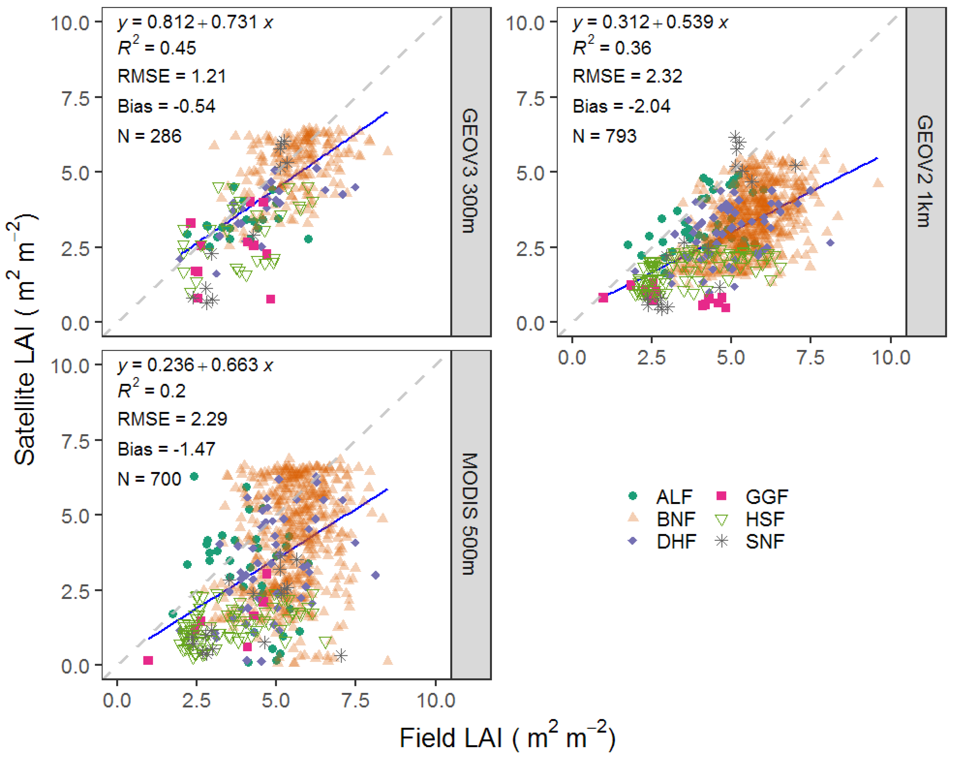
3.1. Accuracy of the LAI Products Magnitude

Satellite derived mean LAI estimates were typically lower than the field measurements, which varied between 3.2 and 5.6 m2 m−2 (Table 2). GEOV3 300 m estimates were 10% lower than field measurements (mean = 4.50 m2 m−2), MODIS 500m were 30% lower (mean = 3.6 m2 m−2 and GEOV2 1 km were 40% lower (mean = 3.07 m2 m−2) (Figure 2; Table 2). LAI mean and relative uncertainty increased with product resolution: GEOV3 300m (0.22, 7%) < MODIS 500 m (0.37, 10%) < GEOV2 1 km (0.56, 19%).
Field mean LAI was best captured by GEOV3 300 m (R2 = 0.45; Figure 3), followed by GEOV2 1 km (R2 = 0.36), and MODIS 500 m (R2 = 0.20) for all of these six forests in this region. This performance varied between forests and all of these products showed the highest R2 (Table 2) for the forests at SNF, which showed more LAI seasonal variation (Figure 2). GEOV3 300 m LAI also had the lowest RMSE and bias (RMSE = 1.21, bias = −0.41) compared with GEOV2 1 km LAI (RMSE = 2.32, bias = −2.04) and MODIS 500m LAI (RMSE = 2.29, bias = −1.47) (Figure 3, Table 2).

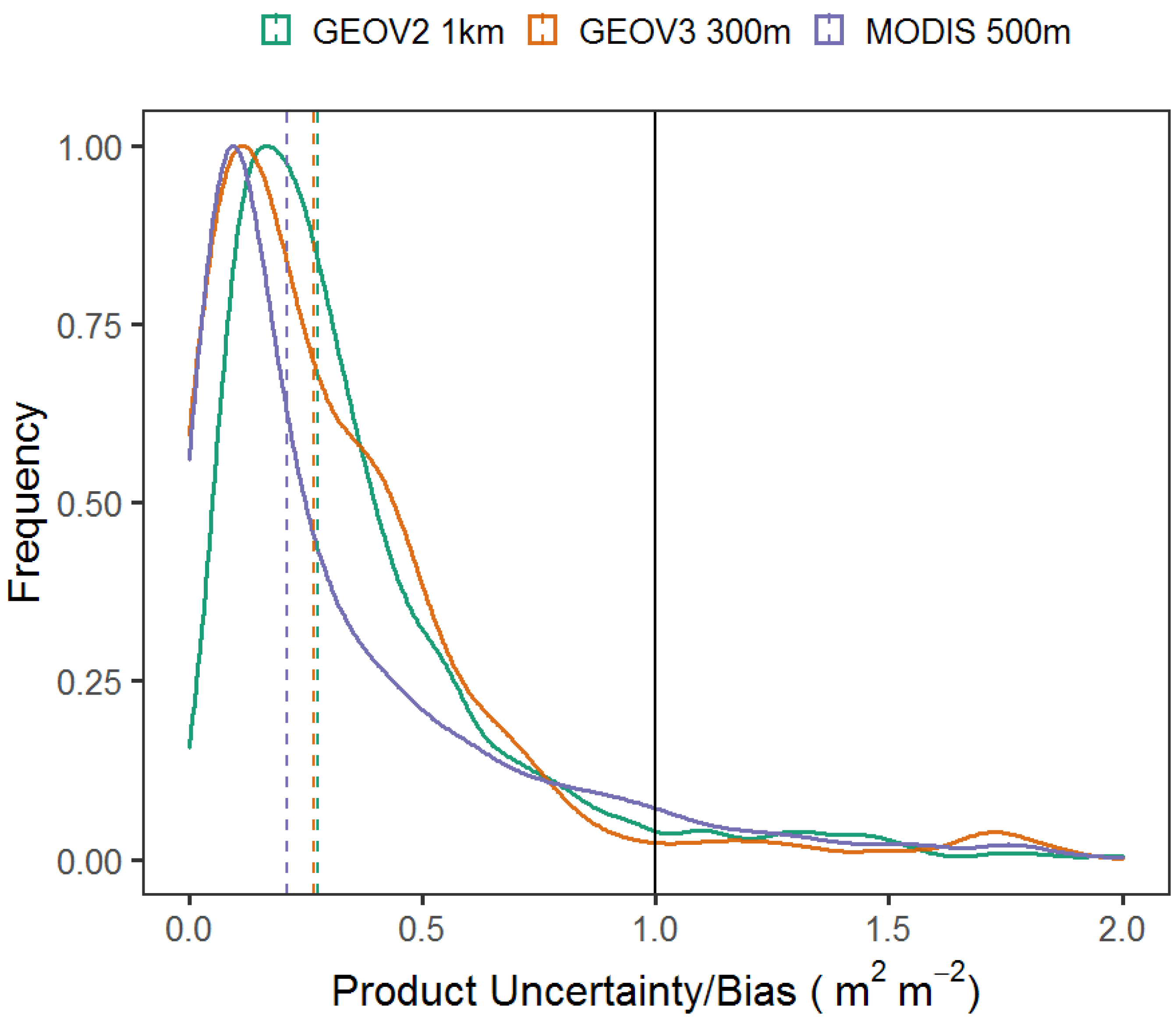
3.2. Robustness of the LAI Products Uncertainty

The magnitude of the reported EO LAI uncertainty is typically smaller than the bias to in situ estimates (Figure 4), here shown as the ratio of uncertainty and reported bias (r), and this result is consistent across forests (Figure S5, Table 2). GEOV3 300 m has the smallest proportion of EO uncertainty estimates below the observed bias (86%) while MODIS 500m LAI and GEOV2 1 km have 87% and 91% of uncertainty estimates below the reported bias. The median ratio indicated similar average skill between both GEOV3 300 m (0.26) and GEOV2 1km LAI products (0.28) and MODIS 500 m LAI products (0.21) (Figure 4, Table 2).

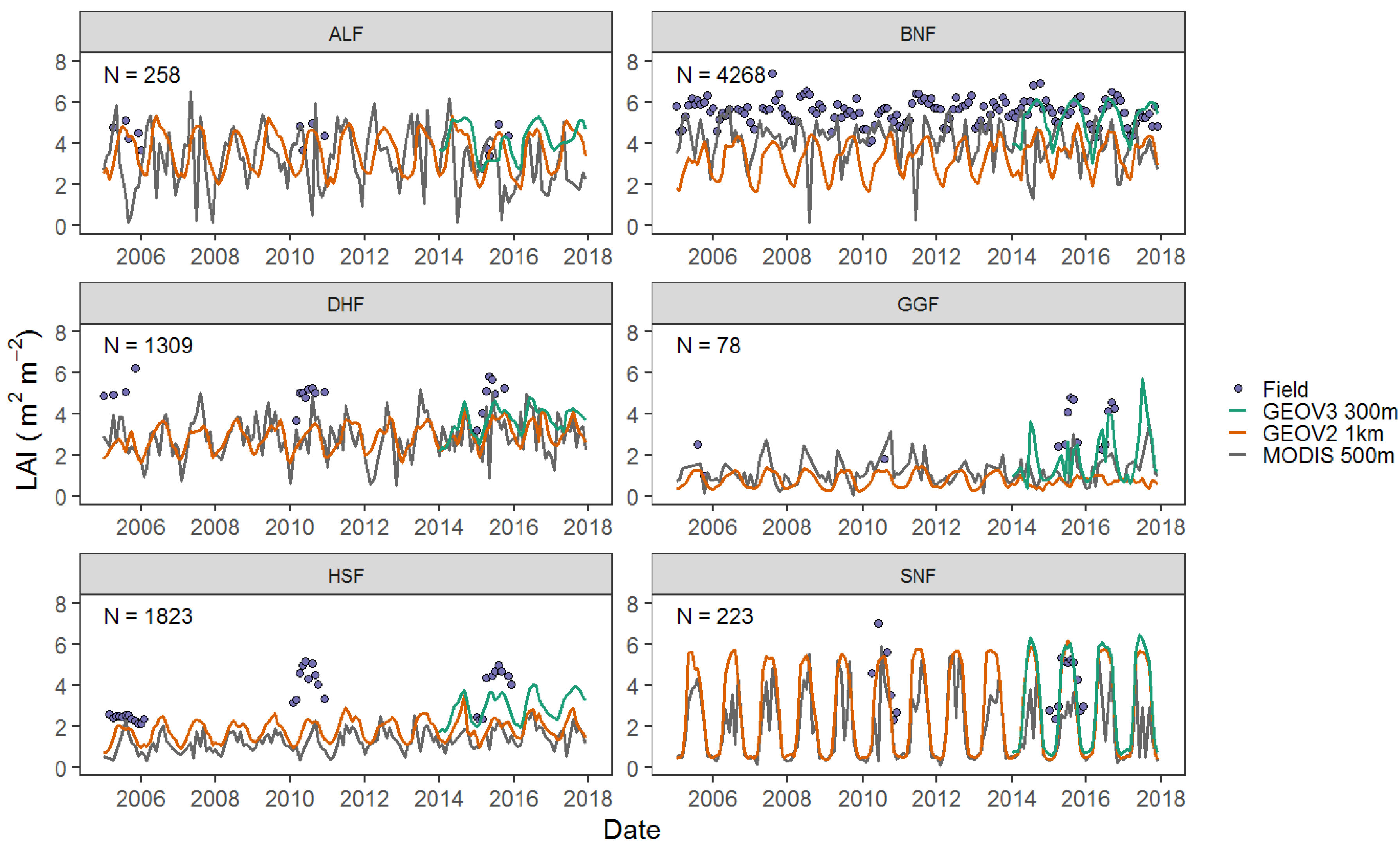
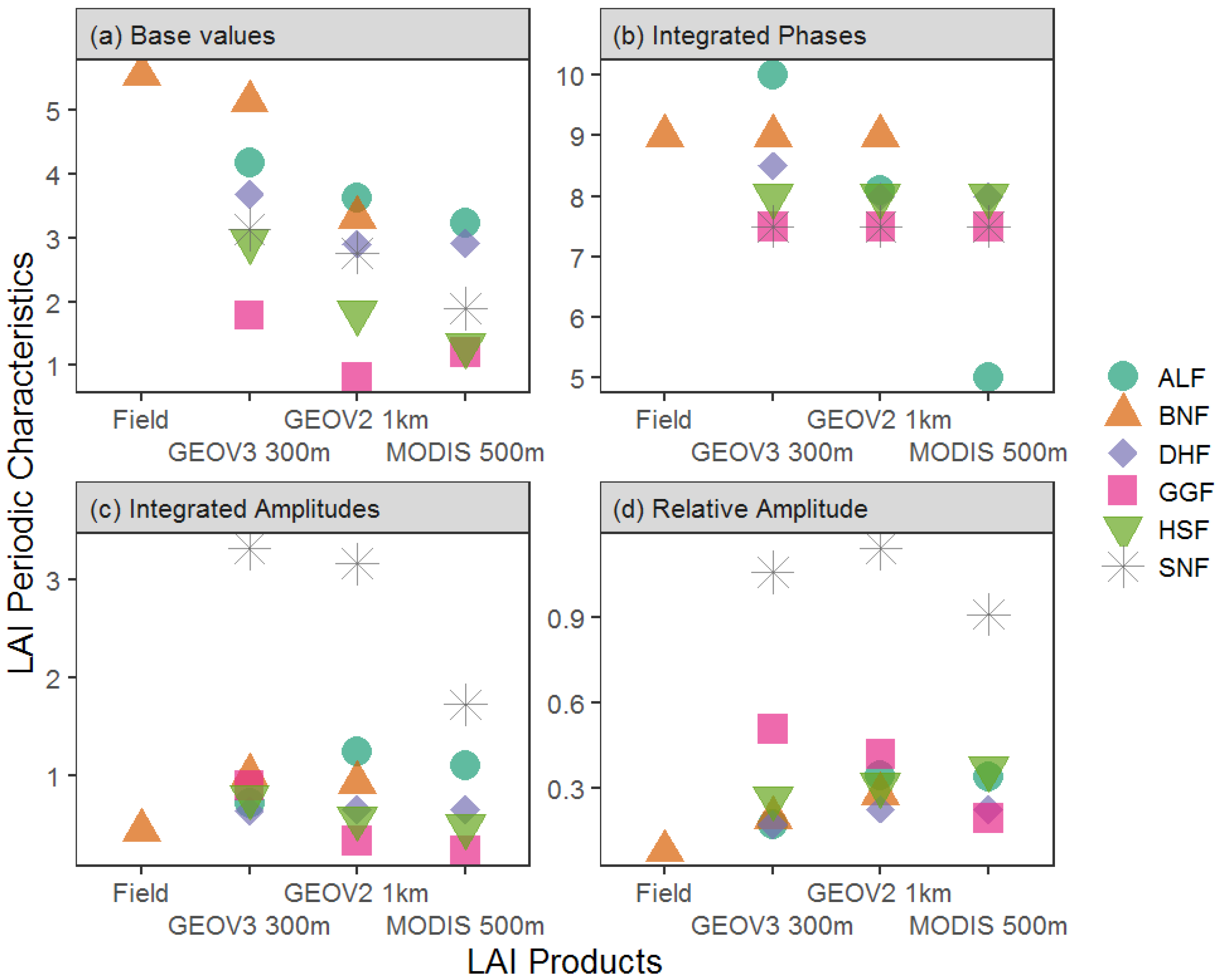
3.3. Validation of the LAI Products Temporal Dynamics

The metaCycle analysis showed that a statistically significant period of 12 months (p < 0.05) is present in the monthly field LAI time series at BNF and in all monthly satellite LAI time series at all sites, except for MODIS 500 m LAI, which showed no significant 12-month periodic characteristics at BNF. Overall, LAI retrieved from GEOV3 300 m showed very close values of the base, phase, amplitude and relative amplitude with the field LAI at BNF (Figure 5). LAI retrieved from GEOV2 1km showed a lower base and amplitude, similar phase, but larger relative amplitude compared with GEOV3 300 m LAI for most sites and the field at BNF (Figure 5). LAI retrieved from MODIS 500 m product showed the lower base values, but had a high variation of phases with one underestimated phase for the forest at ALF compared with the other two LAI products (Figure 5b). The relative amplitude of LAI retrieved from MODIS 500 m is lower for the forest at GGF and SNF, but higher at HSF compared with the other two LAI products (Figure 5c).

3.4. Evaluation of Landcover Heterogeneity

The Landsat data provide a more spatially consistent comparison of surface reflectance against field data of LAI. The results (Figure S6) show that there are significant correlations between NDVI/EVI and LAI across sites, but the effect sizes are small (R2 = 0.1). Thus, the relationships between remotely-sensed NDVI/EVI at the fine resolution and field-measured LAI are less significant than those between LAI products at the coarse resolution and field-measured LAI. The forest cover proportion at the pixel level varied between 38%–100% (Table S3). The landcover data show that LAI retrievals were degraded by the heterogeneity of landcover within product pixels. There was a clear pattern of LAI bias increasing with reductions in the proportions of forest cover at the pixel scale (Figure S7).

4. Discussion

The performance of three EO LAI products was evaluated at six forests across southern China. GEOV3 300 m LAI showed the best fit (R2 = 0.45) and the smallest bias (bias = −0.54) (Figure 3) and the most similar LAI time series seasonal dynamic variation (phase and amplitude) compared with in situ LAI measurements (Figure 5). For the GEOV2 1 km LAI product, its performance had larger bias (Figure 3) and seasonality but similar phases of the LAI time series with the in situ observations compared with GEOV3 300 m LAI products (Figure 3 and Figure 5).
The different performance of the two Copernicus products is likely due to the mismatch of the scaling between the EO pixel size and the field site. LAI is strongly non-linearly related to reflectance, making its estimation from remote sensing observations scale-dependent [76,77]. In contrast, the core operational algorithm (neural network techniques), data filtering and smoothing processes are similar for these two products. There are differences in the method used for temporal compositing, where temporal smoothing and gap filling using a climatology are used for GEOV2 1 km and interpolation applied in GEOV3 300 m) [78]. Differences in the applied gap-filling approach between these two products do not impact our conclusion that resolution is the primary driver of performance improvement at 300 m relative to 1 km, as all gap-filled and interpolated retrievals were removed in our study. The in situ measurements were usually conducted in protected mature forest areas with high plant densities, complex canopy stratums, and rich species diversities (Figure S1, Table S1). However, at coarser spatial resolutions, pixels integrate heterogeneity over a greater diversity of landscapes, habitats, and species, distributed across a variety of stages of growth and succession [79]. Thus, fine resolution GEOV3 300 m LAI product showed lower bias and similar seasonal dynamic variation to the in-situ measurements compared to the higher bias for the GEOV2 1 km LAI product.
For Collection 6 500 m MODIS LAI, our results indicate that this product does not capture the dynamics observed in situ, irrespective of the accuracy of estimated in situ LAI (Figure 3). Furthermore, it does not adequately capture the LAI seasonal dynamics (Figure 5). This result is consistent with two validation studies which both showed MODIS LAI had the poorest performance for the evergreen forests in the south of China [80,81]. The MODIS LAI values for tropical evergreen forests are severely impacted by atmospheric conditions, especially clouds during the growing season (around 42% data are influenced by the cloud in this study, Figure S8), which lead to strong noise in the input reflectance data and affect the retrieval [78]. Additionally, the reflectance saturation usually happened in dense canopies and the main algorithm is sensitive to uncertainties in atmospheric correction, particularly when red and NIR BRFs are saturated [82,83]. This means the reflectance does not contain sufficient information to estimate the LAI value [84] and leads to the instability of the LAI retrievals [14]. All of these may result in the poor performance of representation of evergreen forests in southern China for the MODIS 500 m LAI products. Furthermore, the product does not adequately capture LAI periodic characteristics in comparison to the field data and showed temporal inconsistency with GEOV2 and V3 products (Figure 5). Jiang (2017) also found the large temporal inconsistency between existing global LAI products at a longer time scale [85]. Cammalleri (2019) found GEOV2 fAPAR showed a systematic overestimation of the fAPAR anomalies compared with the MODIS fAPAR and proposed a two-step harmonization procedure to remove this discrepancy [86]. However, the homogenization may alter the magnitude of the original fAPAR time series in an undesirable way. These results highlight the need to validate the temporal consistency between different satellite products and explore more solutions to deal with such inconsistencies. In addition, geolocation uncertainty due to the spatial mismatch could also have influenced validation reliability, As our study sites are not homogeneous and sampling area is consistently smaller than the pixel of remote sensing data, mean or median remotely-sensed LAI values of surrounding 3 × 3 array of pixels [15,87,88] cannot be used for validation. To solve this problem, future field measurements should be conducted at a larger spatial scale and across more homogenous habitats.
Overall, the absolute and relative uncertainty of LAI products tends to be smaller for the fine resolution LAI products (Table 2). Collection 300 m GEOV3 has the smallest absolute uncertainty at around 0.22. Collection1 km GEOV2 has the largest absolute uncertainty at around 0.56. Uncertainty magnitude for Collection 6 500 m MODIS LAI is 0.37. This performance is consistent with the LAI relative uncertainty (Table 2). If compared with the absolute uncertainty requirements (±0.5) and relative uncertainty requirements (20%) set by the GCOS [12], all three products (Collection 300 m GEOV3, 0.22, 5%; Collection 6 500 m MODIS LAI, 0.37, 10%; Collection 1 km GEOV2 0.56, 18%) appear satisfactory. This is consistent with two global studies comparing different EO LAI products (MODIS, CYCLOPES, and GLOBCARBON) at two coarse spatial resolutions (5 km and 1 km). More pixels can meet the absolute uncertainty and relative uncertainty requirements at the spatial resolution of 1 km compared with the 5 km [19,34]. All of these results indicated that the LAI product uncertainty is scale-dependent. The algorithms will produce smaller uncertainty estimated for the LAI values at finer spatial scales. This could make the uncertainty estimates of the fine-resolution products become very conservative.
Changes in LAI error with spatial resolution could be due to vegetation heterogeneity, especially for the forests and scale-dependent reflectance values. However, it is still unclear how product uncertainty changes over different spatial scales. For MODIS, the product uncertainty is the standard deviation over all acceptable solutions of a look-up table (LUT) retrieval method [17]; for Collection 300 m GEOV3 and 1 km GEOV2 LAI products, the quantitative uncertainties (LAI_ERR) are computed as the RMSE between the final dekadal value and the daily NNTs estimates in the compositing period [12,62]. Standardizing different LAI products to the same spatial scale and averaging the LAI and uncertainty for different pixels during the upscaling and resampling process [19,89] could all generate errors [90]. When dealing with different spatial scales, the land surface properties (e.g., land cover proportion, soil properties) could change significantly. Thus, LAI retrieval algorithms are based on inherent empirical assumptions on the distribution of their parameters, which can depart significantly from the actual canopy and soil characteristics [14].
The ratio (r, in Equation (4)) of LAI product uncertainty to the bias of in situ measurements is dramatically lower than the reference value for all of these LAI products (Figure 4, Table 2). This result indicated that none of the three LAI uncertainty products tested here were able to provide a robust estimate for the in-situ measurements. The most promising product is the Collection 300 m GEOV3 LAI; however, while its accuracy is the best, its uncertainty is still too conservative to capture the offset from co-located field LAI measurements. This weakness reflects the complexity of this biome type and highlights that the algorithm used to generate the uncertainty information for these LAI products needs to be improved. For areas of high uncertainties, data producers may need to refine the algorithms and verify the information using additional data sources, particularly in situ data [34]. However, with respect to field data collection, more accurate measurements are also needed to test the results, such as destructive methods or using the litterfall traps. Direct measurement methods obtaining ‘true’ LAI values could also act as a reference to correct the bias and errors in indirect measurement techniques [31].
The accuracy of LAI data retrieved from remote sensing products is very important for a range of earth system models, for which LAI is a key internal variable. LAI uncertainty is particularly critical for model-data fusion in terrestrial carbon cycle studies [91]. The uncertainty produced for the existing remote sensing LAI products in the analysis would further lead to biases in vegetation productivity estimates [92,93,94]. For instance, the saturation of satellite-derived VIs generally results in an underestimation of GPP or NPP in areas with dense vegetation. Using finer resolution remote sensing data in carbon modeling studies could be an effective way to reduce the uncertainty in the estimates of C fluxes and/or stocks, but more robust errors are critical [95].
Uncertainty estimates of the observations are as important as the observations themselves because together they co-determine the outcome of the assimilation systems [96]. Bayesian approaches are commonly used data assimilation systems and the influence of observations are weighted by observational uncertainties. Uncertainties in data are critical as they often determine the outcome of analyses and forecasts [97]. The assimilation process requires clear error quantification for LAI to resolve model results and limit biases [98]. Besides, the presence of bias in a data stream will limit the utility of using multiple observation types in an assimilation framework. Therefore, it is imperative to characterize the error in the observations and understand better the error associated with the direct measurements of LAI to landscape pixel [99]. Our results indicated that none of these LAI uncertainty products are robust and therefore users should consider inflating the existing LAI product uncertainty when using these data sources in data assimilation frameworks [98,100,101] or in other studies for which the uncertainty of the product plays an important role.
One way of solving this spatial mismatch problem is to upscale the field measurements based on its relationship with the plant index retrieved from high-resolution images (e.g., 10–30 m resolution) [102], or using airborne Light Detection and Ranging (LiDAR) [103,104]. However, we failed to find a good relationship between the Landsat based EVI or NDVI and the field measurements (Figure S5). LAI-VI relationships are limited by a number of factors, including vegetation type, sun-surface-sensor geometry, leaf chlorophyll content, background reflectance, and atmospheric quality [31]. Geolocation uncertainties due to spatial mismatch and insufficient overlap data between in situ measurements and good quality Landsat scenes partly lead to this result. Saturation effects occur for both field measurement and spectral plant indices for very dense canopies, which also increases the challenge of upscaling field LAI to generate high-resolution LAI reference maps. In addition, the temporal mismatch between field and Landsat data also contributes to the poor relationship between field and Landsat data. This result may be also associated with the complex forest environments (such as terrain, tree densities, canopy structures, and species diversities) in southern China (Figure S4, Table S1). Thus, their LAI cannot be accurately modeled based on simple spectral indices, even with relatively high resolution (30 m) satellite data. More complex upscaling approaches or those utilizing very high-resolution sensors (e.g., LIDAR) to bridge the scaling gap may yield better results [102,105,106]. In particular, there is an exciting potential for unmanned aerial vehicles to provide critical upscaling information from field to satellite [21].
When using EO LAI products in the absence of reliable validation data, we recommend that the provided uncertainties are treated cautiously. Remote-sensing LAI products require improved algorithms with particular attention given to generating robust uncertainty estimates. New cloud and aerosol detection techniques based on time series and spatial analysis may help to improve the uncertainty products and LAI estimated for evergreen forests [107]. In addition, the new remote-sensing systems such as Global Ecosystem Dynamics Investigation (GEDI) [108], National Aeronautics and Space Administration’s (NASA’s) Ice, Cloud, and land Elevation Satellite-2 (ICESat-2) and Synthetic aperture radar (SAR) provide promising ways to solve cloud coverage issues [109]. Given the importance of data uncertainties (e.g., integration within terrestrial carbon modeling frameworks [92,93,94]), there is an urgent need for robust uncertainty characterization, based on links to in situ observations. The findings in this study are constrained to southern China. Future studies could explore the LAI and error products for other regions, or focus on the seasons where products show the largest uncertainties [19].

5. Conclusions

In this study, we validated three global LAI products and their uncertainty products using ~8000 in situ measurements of LAI from subtropical and tropical forests in the southern China region. The finest resolution product, Collection 300 m GEOV3, performed best, with the lowest RMSE and the lowest bias. It also best captured the temporal dynamics observed in the in-situ dataset, including the magnitude, amplitude, and phases of the LAI time series. Collection 6 500 m MODIS LAI showed the poorest performance and importantly it did not capture the temporal dynamics observed in situ for the forests in this specific region. Critically, for all three LAI products, the accompanying uncertainties were all far smaller than the bias compared to the in situ measurements, indicating that each product uncertainty estimate is not robust. Given the importance of LAI uncertainty in the context of constraining models of carbon cycling and other ecosystem processes, users should use the product’s uncertainty with caution and consider inflating the existing LAI product uncertainty when using it within data assimilation frameworks or other studies in which the uncertainty plays an important role.

Supplementary Materials

The following are available online at https://www.mdpi.com/2072-4292/12/19/3122/s1, Table S1: Detailed forest community information in the southern China region, Table S2: The detailed information for field LAI measurements at each site, Table S3: Distribution of the ratio of EO uncertainty estimates to bias, based on a comparison against in situ LAI measurements, Figure S1: Forest appearance for each forest in this study in the southern China region, Figure S2: TOPO30 DEM (1 km) in the China region. Figure S3: Location of the sampling subplots and the GEOV2 1 km LAI pixels showed on the Landsat EVI scenes for different sites, Figure S4: Location of the sampling subplots and the GEOV2 1km LAI pixels showed on the SARTM 90 m DEM images for different sites. Figure S5: Frequency distribution of the ratio of LAI products uncertainty with LAI products’ bias against the in situ measurements for different sites. Figure S6: Regression analyses between the Landsat EVI/NDVI values and the field observed LAI values at sampling subplots, Figure S7: Regression analyses between the proportion of forests cover (LAI pixel level) and the remotely sensed LAI bias against the field measured LAI for different LAI products, Figure S8: Summary of the dates for the MODIS LAI pixels which were influenced by the cloud in this study.

Author Contributions

Conceptualization, Y.Z. and M.W.; methodology, Y.Z., M.W., T.L.S., and D.T.M.; formal analysis, T.L.S. and S.F.-P. and D.T.M.; writing—original draft preparation, Y.Z. and M.W.; writing—review and editing, M.W., X.C., T.L.S., D.T.M., S.F.-P., and Y.Z. All authors have read and agreed to the published version of the manuscript.

Funding

This research was funded by the National Natural Science Foundation of China under grant number 41771049 and NCEO, CSSP Newton Fund, and China Scholarship Council.

Acknowledgments

The authors thank all the workers in the Chinese Ecosystem Research Network for field data collection and database establishment.

Conflicts of Interest

The authors declare no conflict of interest.

References

  1. Anav, A.; Murray-Tortarolo, G.; Friedlingstein, P.; Sitch, S.; Piao, S.; Zhu, Z. Evaluation of land surface models in reproducing satellite Derived leaf area index over the high-latitude northern hemisphere. Part II: Earth system models. Remote Sens. 2013, 5, 3637–3661. [Google Scholar] [CrossRef] [Green Version]
  2. Mahowald, N.; Lo, F.; Zheng, Y.; Harrison, L.; Funk, C.; Lombardozzi, D.; Goodale, C. Projections of leaf area index in earth system models. Earth Syst. Dynam. 2016, 7, 211–229. [Google Scholar] [CrossRef] [Green Version]
  3. Williams, M.; Richardson, A.D.; Reichstein, M.; Stoy, P.C.; Peylin, P.; Verbeeck, H.; Carvalhais, N.; Jung, M.; Hollinger, D.Y.; Kattge, J. Improving land surface models with FLUXNET data. Biogeosciences 2009, 6, 2785. [Google Scholar] [CrossRef] [Green Version]
  4. Asner, G.P.; Scurlock, J.M.; Hicke, A.J. Global synthesis of leaf area index observations: Implications for ecological and remote sensing studies. Glob. Ecol. Biogeogr. 2003, 12, 191–205. [Google Scholar] [CrossRef] [Green Version]
  5. Fang, H.; Liang, S.; Hoogenboom, G. Integration of MODIS LAI and vegetation index products with the CSM–CERES–Maize model for corn yield estimation. Int. J. Remote Sens. 2011, 32, 1039–1065. [Google Scholar] [CrossRef]
  6. Richardson, A.D.; Dail, D.B.; Hollinger, D. Leaf area index uncertainty estimates for model–data fusion applications. Agric. For. Meteorol. 2011, 151, 1287–1292. [Google Scholar] [CrossRef]
  7. Asaadi, A.; Arora, V.K.; Melton, J.R.; Bartlett, P. An improved parameterization of leaf area index (LAI) seasonality in the Canadian Land Surface Scheme (CLASS) and Canadian Terrestrial Ecosystem Model (CTEM) modelling framework. Biogeosciences 2018, 15, 6885–6907. [Google Scholar] [CrossRef] [Green Version]
  8. Tum, M.; Günther, K.P.; Böttcher, M.; Baret, F.; Bittner, M.; Brockmann, C.; Weiss, M. Global gap-free MERIS LAI time series (2002–2012). Remote Sens. 2016, 8, 69. [Google Scholar] [CrossRef] [Green Version]
  9. Gonsamo, A.; Chen, J.M. Improved LAI Algorithm Implementation to MODIS Data by Incorporating Background, Topography, and Foliage Clumping Information. IEEE Trans. Geosci. Remote Sens. 2014, 52, 1076–1088. [Google Scholar] [CrossRef]
  10. Myneni, R.; Knyazikhin, Y.; Park, T. MOD15A2H MODIS/Terra Leaf Area Index/FPAR 8-Day L4 Global 500 m SIN Grid V006 [Data set]. NASA EOSDIS Land Processes DAAC. 2015. Available online: https://doi.org/10.5067/MODIS/MCD15A2H.006 (accessed on 15 September 2020).
  11. Verger, A.; Baret, F.; Weiss, M. Near Real-Time Vegetation Monitoring at Global Scale. IEEE J. Sel. Top. Appl. Earth Obs. Remote Sens. 2014, 7, 3473–3481. [Google Scholar] [CrossRef]
  12. Baret, F.; Weiss, M.; Verger, A.; Smets, B. Atbd for Lai, Fapar and Fcover From Proba-V Products at 300m Resolution (Geov3); INRA: Paris, France, 2016. [Google Scholar]
  13. Williams, M.; Rastetter, E.B.; Shaver, G.R.; Hobbie, J.E.; Carpino, E.; Kwiatkowski, B.L. Primary production of an arctic watershed: An uncertainty analysis. Ecol. Appl. 2001, 11, 1800–1816. [Google Scholar] [CrossRef]
  14. Garrigues, S.; Lacaze, R.; Baret, F.; Morisette, J.; Weiss, M.; Nickeson, J.; Fernandes, R.; Plummer, S.; Shabanov, N.; Myneni, R. Validation and intercomparison of global Leaf Area Index products derived from remote sensing data. J. Geophys. Res. Biogeosci. 2008, 113. [Google Scholar] [CrossRef]
  15. Weiss, M.; Baret, F.; Garrigues, S.; Lacaze, R. LAI and fAPAR CYCLOPES global products derived from VEGETATION. Part 2: Validation and comparison with MODIS collection 4 products. Remote Sens. Environ. 2007, 110, 317–331. [Google Scholar] [CrossRef]
  16. Baret, F.; Hagolle, O.; Geiger, B.; Bicheron, P.; Miras, B.; Huc, M.; Berthelot, B.; Niño, F.; Weiss, M.; Samain, O.; et al. LAI, fAPAR and fCover CYCLOPES global products derived from VEGETATION: Part 1: Principles of the algorithm. Remote Sens. Environ. 2007, 110, 275–286. [Google Scholar] [CrossRef] [Green Version]
  17. Knyazikhin, Y. MODIS Leaf Area Index (LAI) and Fraction of Photosynthetically Active Radiation Absorbed by Vegetation (FPAR) Product (MOD 15) Algorithm Theoretical Basis Document. 1999. Available online: https://modis.gsfc.nasa.gov/data/atbd/atbd_mod15.pdf (accessed on 15 September 2020).
  18. Pinty, B.; Andredakis, I.; Clerici, M.; Kaminski, T.; Taberner, M.; Verstraete, M.; Gobron, N.; Plummer, S.; Widlowski, J.L. Exploiting the MODIS albedos with the Two-stream Inversion Package (JRC-TIP): 1. Effective leaf area index, vegetation, and soil properties. J. Geophys. Res. Atmos. 2011, 116. [Google Scholar] [CrossRef]
  19. Fang, H.; Jiang, C.; Li, W.; Wei, S.; Baret, F.; Chen, J.M.; Garcia-Haro, J.; Liang, S.; Liu, R.; Myneni, R.B.; et al. Characterization and intercomparison of global moderate resolution leaf area index (LAI) products: Analysis of climatologies and theoretical uncertainties. J. Geophys. Res. Biogeosci. 2013, 118, 529–548. [Google Scholar] [CrossRef]
  20. GCOS. Systematic Observation Requirements for Satellite-Based Products for Climate. 2011 Update Supplemetnatl Details to the Satellite 39 Based Component og the Implementation Plan for the Global Observing System for Climate in Support of the UNFCCC (2010 Update); Technical Report; World Meteorological Organisation (WMO) 7 bis: Geneva, Switzerland, 2011. [Google Scholar]
  21. Revill, A.; Florence, A.; MacArthur, A.; Hoad, S.; Rees, R.; Williams, M. Quantifying Uncertainty and Bridging the Scaling Gap in the Retrieval of Leaf Area Index by Coupling Sentinel-2 and UAV Observations. Remote Sens. 2020, 12, 1843. [Google Scholar] [CrossRef]
  22. Williams, M.; Bell, R.; Spadavecchia, L.; Street, L.E.; Van Wijk, M.T. Upscaling leaf area index in an Arctic landscape through multiscale observations. Glob. Chang. Biol. 2008, 14, 1517–1530. [Google Scholar] [CrossRef] [Green Version]
  23. Wang, Q.; Tenhunen, J.; Dinh, N.Q.; Reichstein, M.; Otieno, D.; Granier, A.; Pilegarrd, K. Evaluation of seasonal variation of MODIS derived leaf area index at two European deciduous broadleaf forest sites. Remote Sens. Environ. 2005, 96, 475–484. [Google Scholar] [CrossRef]
  24. Wang, J.; Wu, C.; Wang, X.; Zhang, X. A new algorithm for the estimation of leaf unfolding date using MODIS data over China’s terrestrial ecosystems. ISPRS J. Photogramm. Remote Sens. 2019, 149, 77–90. [Google Scholar] [CrossRef]
  25. Kou, W.; Liang, C.; Wei, L.; Hernandez, A.J.; Yang, X. Phenology-based method for mapping tropical evergreen forests by integrating of MODIS and landsat imagery. Forests 2017, 8, 34. [Google Scholar]
  26. Clark, D.A. Sources or sinks? The responses of tropical forests to current and future climate and atmospheric composition. Philos. Trans. R. Soc. Lond. B Biol. Sci. 2004, 359, 477–491. [Google Scholar] [PubMed] [Green Version]
  27. Miller, S.D.; Goulden, M.L.; Hutyra, L.R.; Keller, M.; Saleska, S.R.; Wofsy, S.C.; Figueira, A.M.S.; da Rocha, H.R.; de Camargo, P.B. Reduced impact logging minimally alters tropical rainforest carbon and energy exchange. Proc. Natl. Acad. Sci. USA 2011, 108, 19431–19435. [Google Scholar] [CrossRef] [PubMed] [Green Version]
  28. Tang, A.C.I.; Stoy, P.C.; Hirata, R.; Musin, K.K.; Aeries, E.B.; Wenceslaus, J.; Shimizu, M.; Melling, L. The exchange of water and energy between a tropical peat forest and the atmosphere: Seasonal trends and comparison against other tropical rainforests. Sci. Total Environ. 2019, 683, 166–175. [Google Scholar] [CrossRef]
  29. Heiskanen, J.; Korhonen, L.; Hietanen, J.; Pellikka, P.K.E. Use of airborne lidar for estimating canopy gap fraction and leaf area index of tropical montane forests. Int. J. Remote Sens. 2015, 36, 2569–2583. [Google Scholar] [CrossRef]
  30. Piao, S.; Liu, Q.; Chen, A.; Janssens, I.A.; Fu, Y.; Dai, J.; Liu, L.; Lian, X.; Shen, M.; Zhu, X. Plant phenology and global climate change: Current progresses and challenges. Glob. Chang. Biol. 2019, 25, 1922–1940. [Google Scholar]
  31. Fang, H.; Baret, F.; Plummer, S.; Schaepman-Strub, G. An overview of global leaf area index (LAI): Methods, products, validation, and applications. Rev. Geophys. 2019, 57, 739–799. [Google Scholar]
  32. Chhabra, A.; Panigrahy, S. Analysis of spatio-temporal patterns of leaf area index in different forest types of India using high temporal remote sensing data. Int. Arch. Photogramm. Remote Sens. Spat. Inf. Sci. 2011, 38, W20. [Google Scholar]
  33. Olivas, P.C.; Oberbauer, S.F.; Clark, D.B.; Clark, D.A.; Ryan, M.G.; O’Brien, J.J.; Ordonez, H. Comparison of direct and indirect methods for assessing leaf area index across a tropical rain forest landscape. Agric. For. Meteorol. 2013, 177, 110–116. [Google Scholar]
  34. Fang, H.; Wei, S.; Jiang, C.; Scipal, K. Theoretical uncertainty analysis of global MODIS, CYCLOPES, and GLOBCARBON LAI products using a triple collocation method. Remote Sens. Environ. 2012, 124, 610–621. [Google Scholar]
  35. Huete, A.R.; Didan, K.; Shimabukuro, Y.E.; Ratana, P.; Saleska, S.R.; Hutyra, L.R.; Yang, W.; Nemani, R.R.; Myneni, R. Amazon rainforests green-up with sunlight in dry season. Geophys. Res. Lett. 2006, 33. [Google Scholar] [CrossRef] [Green Version]
  36. Wagner, F.H.; Hérault, B.; Rossi, V.; Hilker, T.; Maeda, E.E.; Sanchez, A.; Lyapustin, A.I.; Galvão, L.S.; Wang, Y.; Aragao, L.E. Climate drivers of the Amazon forest greening. PLoS ONE 2017, 12, e0180932. [Google Scholar] [CrossRef] [PubMed] [Green Version]
  37. Wu, J.; Kobayashi, H.; Stark, S.C.; Meng, R.; Guan, K.; Tran, N.N.; Gao, S.; Yang, W.; Restrepo-Coupe, N.; Miura, T. Biological processes dominate seasonality of remotely sensed canopy greenness in an Amazon evergreen forest. New Phytol. 2018, 217, 1507–1520. [Google Scholar] [CrossRef] [PubMed] [Green Version]
  38. Wu, J.; Albert, L.P.; Lopes, A.P.; Restrepo-Coupe, N.; Hayek, M.; Wiedemann, K.T.; Guan, K.; Stark, S.C.; Christoffersen, B.; Prohaska, N. Leaf development and demography explain photosynthetic seasonality in Amazon evergreen forests. Science 2016, 351, 972–976. [Google Scholar] [CrossRef] [PubMed] [Green Version]
  39. Tang, H.; Dubayah, R. Light-driven growth in Amazon evergreen forests explained by seasonal variations of vertical canopy structure. Proc. Natl. Acad. Sci. USA 2017, 114, 2640–2644. [Google Scholar] [CrossRef] [Green Version]
  40. Yan, D.; Zhang, X.; Yu, Y.; Guo, W. A comparison of tropical rainforest phenology retrieved from geostationary (seviri) and polar-orbiting (modis) sensors across the congo basin. IEEE Trans. Geosci. Remote Sens. 2016, 54, 4867–4881. [Google Scholar] [CrossRef] [Green Version]
  41. Adole, T.; Dash, J.; Atkinson, P.M. A systematic review of vegetation phenology in Africa. Ecol. Inform. 2016, 34, 117–128. [Google Scholar] [CrossRef]
  42. Ryan, C.M.; Williams, M.; Grace, J.; Woollen, E.; Lehmann, C.E. Pre-rain green-up is ubiquitous across southern tropical Africa: Implications for temporal niche separation and model representation. New Phytol. 2017, 213, 625–633. [Google Scholar] [CrossRef] [Green Version]
  43. Piao, S.; Fang, J.; Zhou, L.; Ciais, P.; Zhu, B. Variations in satellite-derived phenology in China’s temperate vegetation. Glob. Chang. Biol. 2006, 12, 672–685. [Google Scholar] [CrossRef]
  44. Wu, C.; Hou, X.; Peng, D.; Gonsamo, A.; Xu, S. Land surface phenology of China’s temperate ecosystems over 1999–2013: Spatial–temporal patterns, interaction effects, covariation with climate and implications for productivity. Agric. For. Meteorol. 2016, 216, 177–187. [Google Scholar] [CrossRef]
  45. Liu, Q.; Fu, Y.H.; Zeng, Z.; Huang, M.; Li, X.; Piao, S. Temperature, precipitation, and insolation effects on autumn vegetation phenology in temperate China. Glob. Chang. Biol. 2016, 22, 644–655. [Google Scholar] [CrossRef] [PubMed]
  46. Ge, Q.; Dai, J.; Cui, H.; Wang, H. Spatiotemporal Variability in Start and End of Growing Season in China Related to Climate Variability. Remote Sens. 2016, 8, 433. [Google Scholar] [CrossRef] [Green Version]
  47. Zhu, H. The Tropical Forests of Southern China and Conservation of Biodiversity. Bot. Rev. 2017, 83, 87–105. [Google Scholar] [CrossRef]
  48. Wu, J.; Lin, W.; Peng, X.; Liu, W. A review of forest resources and forest biodiversity evaluation system in China. Int. J. Res. 2013, 2013. [Google Scholar] [CrossRef] [Green Version]
  49. Piao, S.; Fang, J.; Ciais, P.; Peylin, P.; Huang, Y.; Sitch, S.; Wang, T. The carbon balance of terrestrial ecosystems in China. Nature 2009, 458, 1009–1013. [Google Scholar] [CrossRef]
  50. Tang, X.; Zhao, X.; Bai, Y.; Tang, Z.; Wang, W.; Zhao, Y.; Wan, H.; Xie, Z.; Shi, X.; Wu, B. Carbon pools in China’s terrestrial ecosystems: New estimates based on an intensive field survey. Proc. Natl. Acad. Sci. USA 2018, 115, 4021–4026. [Google Scholar] [CrossRef] [PubMed] [Green Version]
  51. Justice, C.; Belward, A.; Morisette, J.; Lewis, P.; Privette, J.; Baret, F. 2000: Developments in the ‘validation’of satellite sensor products for the study of the land surface. Int. J. Remote Sens. 2000, 21, 3383–3390. [Google Scholar]
  52. Morisette, J.T.; Baret, F.; Privette, J.L.; Myneni, R.B.; Nickeson, J.E.; Garrigues, S.; Shabanov, N.V.; Weiss, M.; Fernandes, R.A.; Leblanc, S.G. Validation of global moderate-resolution LAI products: A framework proposed within the CEOS land product validation subgroup. IEEE Trans. Geosci. Remote Sens. 2006, 44, 1804–1817. [Google Scholar] [CrossRef] [Green Version]
  53. Post, H.; Hendricks Franssen, H.J.; Han, X.; Baatz, R.; Montzka, C.; Schmidt, M.; Vereecken, H. Evaluation and uncertainty analysis of regional-scale CLM4.5 net carbon flux estimates. Biogeosciences 2018, 15, 187–208. [Google Scholar] [CrossRef] [Green Version]
  54. Rüdiger, C.; Albergel, C.; Mahfouf, J.F.; Calvet, J.C.; Walker, J.P. Evaluation of the observation operator Jacobian for leaf area index data assimilation with an extended Kalman filter. J. Geophys. Res. Atmos. 2010, 115. [Google Scholar] [CrossRef]
  55. Viskari, T.; Hardiman, B.; Desai, A.R.; Dietze, M.C. Model-data assimilation of multiple phenological observations to constrain and predict leaf area index. Ecol. Appl. 2015, 25, 546–558. [Google Scholar] [CrossRef]
  56. Fu, B.; Li, S.; Yu, X.; Yang, P.; Yu, G.; Feng, R.; Zhuang, X. Chinese ecosystem research network: Progress and perspectives. Ecol. Complex. 2010, 7, 225–233. [Google Scholar] [CrossRef]
  57. Yu, G.; Chen, Z.; Piao, S.; Peng, C.; Ciais, P.; Wang, Q.; Li, X.; Zhu, X. High carbon dioxide uptake by subtropical forest ecosystems in the East Asian monsoon region. Proc. Natl. Acad. Sci. USA 2014, 111, 4910–4915. [Google Scholar] [CrossRef] [PubMed] [Green Version]
  58. Peel, M.C.; Finlayson, B.L.; McMahon, T.A. Updated world map of the Köppen-Geiger climate classification. Eur. Geosci. Union 2007, 4, 439–473. [Google Scholar]
  59. Li-Cor, I. LAI-2000 Plant Canopy Analyzer Instruction Manual; LI-COR Inc.: Lincoln, NE, USA, 1992. [Google Scholar]
  60. Wu, D.; Wei, W.; Zhang, S. Protocols for Standard Biological Observation and Measurement in Terrestrial Ecosystems; China Environmental Science Pres: Beijing, China, 2007. [Google Scholar]
  61. Knyazikhin, Y.; Martonchik, J.; Myneni, R.B.; Diner, D.; Running, S.W. Synergistic algorithm for estimating vegetation canopy leaf area index and fraction of absorbed photosynthetically active radiation from MODIS and MISR data. J. Geophys. Res. Atmos. 1998, 103, 32257–32275. [Google Scholar] [CrossRef] [Green Version]
  62. Verger, A.; Baret, F.; Weiss, M. Atbd for Lai, Fapar and Fcover from Proba-V Products Collection 1km Version 2; 2019, Issue I1.41. Available online: https://land.copernicus.eu/global/sites/cgls.vito.be/files/products/CGLOPS1_ATBD_LAI1km-V2_I1.41.pdf (accessed on 15 April 2020).
  63. Masek, J.G.; Vermote, E.F.; Saleous, N.E.; Wolfe, R.; Hall, F.G.; Huemmrich, K.F.; Gao, F.; Kutler, J.; Lim, T.-K. A Landsat surface reflectance dataset for North America, 1990–2000. IEEE Geosci. Remote Sens. Lett. 2006, 3, 68–72. [Google Scholar] [CrossRef]
  64. Vermote, E.; Justice, C.; Claverie, M.; Franch, B. Preliminary analysis of the performance of the Landsat 8/OLI land surface reflectance product. Remote Sens. Environ. 2016, 185, 46–56. [Google Scholar] [CrossRef]
  65. Zanter, K.; Department of the Interior, U.S. Geological Survey. Landsat 4-7 Surface Reflectance (LEDAPS) Product Guide. Version 2.0. 2019, EROS, Sioux Falls, South Dakota. Available online: https://www.usgs.gov/media/files/landsat-4-7-surface-reflectance-code-ledaps-product-guide (accessed on 15 September 2020).
  66. Zanter, K.; Department of the Interior, U.S. Geological Survey. Landsat 8 Surface Reflectance Code (LASRC) Product Guide. Version 2.0. 2019, EROS, Sioux Falls, South Dakota. Available online: https://www.usgs.gov/media/files/land-surface-reflectance-code-lasrc-product-guide (accessed on 15 September 2020).
  67. USGS. GTOPO30: Global 30 Arc-Seconds Digital Elevation Model [Data Set]. Available online: https://www.usgs.gov/centers/eros/science/usgs-eros-archive-digital-elevation-global-30-arc-second-elevation-gtopo30?qt-science_center_objects=0#qt-science_center_objects (accessed on 15 September 2020).
  68. Reuter, H.I.; Nelson, A.; Jarvis, A. An evaluation of void-filling interpolation methods for SRTM data. Int. J. Geogr. Inf. Sci. 2007, 21, 983–1008. [Google Scholar] [CrossRef]
  69. Jun, C.; Ban, Y.; Li, S. Open access to Earth land-cover map. Nature 2014, 514, 434. [Google Scholar] [CrossRef] [Green Version]
  70. Wu, G.; Anafi, R.C.; Hughes, M.E.; Kornacker, K.; Hogenesch, J.B. MetaCycle: An integrated R package to evaluate periodicity in large scale data. Bioinformatics 2016, 32, 3351–3353. [Google Scholar] [CrossRef] [Green Version]
  71. Yang, R.; Su, Z. Analyzing circadian expression data by harmonic regression based on autoregressive spectral estimation. Bioinformatics 2010, 26, i168–i174. [Google Scholar] [CrossRef] [PubMed] [Green Version]
  72. Hughes, M.E.; Hogenesch, J.B.; Kornacker, K. JTK_CYCLE: An efficient nonparametric algorithm for detecting rhythmic components in genome-scale data sets. J. Biol. Rhythms 2010, 25, 372–380. [Google Scholar] [CrossRef] [PubMed]
  73. Glynn, E.F.; Chen, J.; Mushegian, A.R. Detecting periodic patterns in unevenly spaced gene expression time series using Lomb–Scargle periodograms. Bioinformatics 2006, 22, 310–316. [Google Scholar] [CrossRef] [PubMed] [Green Version]
  74. R Core Team. R: A Language and Environment for Statistical Computing; R Foundation for Statistical Computing: Vienna, Austria, 2017; Available online: https://www.r-project.org/ (accessed on 3 December 2018).
  75. Hijmans, R.J.; Van Etten, J.; Cheng, J.; Mattiuzzi, M.; Sumner, M.; Greenberg, J.A.; Lamigueiro, O.P.; Bevan, A.; Racine, E.B.; Shortridge, A. Package ‘raster’. R package version 2.5-8 (2015).
  76. Weiss, M.; Baret, F.; Smith, G.; Jonckheere, I.; Coppin, P. Review of methods for in situ leaf area index (LAI) determination: Part II. Estimation of LAI, errors and sampling. Agric. For. Meteorol. 2004, 121, 37–53. [Google Scholar] [CrossRef]
  77. Garrigues, S.; Allard, D.; Baret, F.; Weiss, M. Influence of landscape spatial heterogeneity on the non-linear estimation of leaf area index from moderate spatial resolution remote sensing data. Remote Sens. Environ. 2006, 105, 286–298. [Google Scholar] [CrossRef]
  78. Fuster, B.; Sánchez-Zapero, J.; Camacho, F.; García-Santos, V.; Verger, A.; Lacaze, R.; Weiss, M.; Baret, F.; Smets, B. Quality Assessment of PROBA-V LAI, fAPAR and fCOVER Collection 300 m Products of Copernicus Global Land Service. Remote Sens. 2020, 12, 1017. [Google Scholar] [CrossRef] [Green Version]
  79. Nagendra, H. Using remote sensing to assess biodiversity. Int. J. Remote Sens. 2001, 22, 2377–2400. [Google Scholar] [CrossRef]
  80. Liu, Z.; Shao, Q.; Liu, J. The Performances of MODIS-GPP and -ET Products in China and Their Sensitivity to Input Data (FPAR/LAI). Remote Sens. 2015, 7, 135–152. [Google Scholar] [CrossRef]
  81. Li, X.; Lu, H.; Yu, L.; Yang, K. Comparison of the spatial characteristics of four remotely sensed leaf area index products over China: Direct validation and relative uncertainties. Remote Sens. 2018, 10, 148. [Google Scholar] [CrossRef] [Green Version]
  82. Shabanov, N.V.; Huang, D.; Yang, W.; Tan, B.; Knyazikhin, Y.; Myneni, R.B.; Ahl, D.E.; Gower, S.T.; Huete, A.R.; Aragão, L.E.O. Analysis and optimization of the MODIS leaf area index algorithm retrievals over broadleaf forests. IEEE Trans. Geosci. Remote Sens. 2005, 43, 1855–1865. [Google Scholar] [CrossRef] [Green Version]
  83. Yang, W.; Shabanov, N.; Huang, D.; Wang, W.; Dickinson, R.; Nemani, R.; Knyazikhin, Y.; Myneni, R. Analysis of leaf area index products from combination of MODIS Terra and Aqua data. Remote Sens. Environ. 2006, 104, 297–312. [Google Scholar] [CrossRef]
  84. Yan, K.; Park, T.; Yan, G.; Chen, C.; Yang, B.; Liu, Z.; Nemani, R.R.; Knyazikhin, Y.; Myneni, R.B. Evaluation of MODIS LAI/FPAR Product Collection 6. Part 1: Consistency and Improvements. Remote Sens. 2016, 8, 359. [Google Scholar] [CrossRef] [Green Version]
  85. Jiang, C.; Ryu, Y.; Fang, H.; Myneni, R.; Claverie, M.; Zhu, Z. Inconsistencies of interannual variability and trends in long-term satellite leaf area index products. Glob. Chang. Biol. 2017, 23, 4133–4146. [Google Scholar] [CrossRef] [PubMed]
  86. Cammalleri, C.; Verger, A.; Lacaze, R.; Vogt, J. Harmonization of GEOV2 fAPAR time series through MODIS data for global drought monitoring. Int. J. Appl. Earth Obs. Geoinf. 2019, 80, 1–12. [Google Scholar] [CrossRef] [PubMed]
  87. Pisek, J.; Chen, J.M.; Alikas, K.; Deng, F. Impacts of including forest understory brightness and foliage clumping information from multiangular measurements on leaf area index mapping over North America. J. Geophys. Res. Biogeosci. 2010, 115. [Google Scholar] [CrossRef] [Green Version]
  88. Verger, A.; Baret, F.; Weiss, M. Performances of neural networks for deriving LAI estimates from existing CYCLOPES and MODIS products. Remote Sens. Environ. 2008, 112, 2789–2803. [Google Scholar] [CrossRef]
  89. Claverie, M.; Vermote, E.F.; Weiss, M.; Baret, F.; Hagolle, O.; Demarez, V. Validation of coarse spatial resolution LAI and FAPAR time series over cropland in southwest France. Remote Sens. Environ. 2013, 139, 216–230. [Google Scholar] [CrossRef]
  90. Tian, Y.; Wang, Y.; Zhang, Y.; Knyazikhin, Y.; Bogaert, J.; Myneni, R.B. Radiative transfer based scaling of LAI retrievals from reflectance data of different resolutions. Remote Sens. Environ. 2003, 84, 143–159. [Google Scholar] [CrossRef]
  91. Bloom, A.A.; Exbrayat, J.-F.; Van Der Velde, I.R.; Feng, L.; Williams, M. The decadal state of the terrestrial carbon cycle: Global retrievals of terrestrial carbon allocation, pools, and residence times. Proc. Natl. Acad. Sci. USA 2016, 113, 1285–1290. [Google Scholar] [CrossRef] [Green Version]
  92. Raupach, M.R.; Rayner, P.J.; Barrett, D.J.; DeFries, R.S.; Heimann, M.; Ojima, D.S.; Quegan, S.; Schmullius, C.C. Model–data synthesis in terrestrial carbon observation: Methods, data requirements and data uncertainty specifications. Glob. Chang. Biol. 2005, 11, 378–397. [Google Scholar] [CrossRef]
  93. Xie, X.; Li, A.; Jin, H.; Tan, J.; Wang, C.; Lei, G.; Zhang, Z.; Bian, J.; Nan, X. Assessment of five satellite-derived LAI datasets for GPP estimations through ecosystem models. Sci. Total Environ. 2019, 690, 1120–1130. [Google Scholar] [CrossRef] [PubMed]
  94. Liu, Y.; Xiao, J.; Ju, W.; Zhu, G.; Wu, X.; Fan, W.; Li, D.; Zhou, Y. Satellite-derived LAI products exhibit large discrepancies and can lead to substantial uncertainty in simulated carbon and water fluxes. Remote Sens. Environ. 2018, 206, 174–188. [Google Scholar] [CrossRef]
  95. Xiao, J.; Chevallier, F.; Gomez, C.; Guanter, L.; Hicke, J.A.; Huete, A.R.; Ichii, K.; Ni, W.; Pang, Y.; Rahman, A.F. Remote sensing of the terrestrial carbon cycle: A review of advances over 50 years. Remote Sens. Environ. 2019, 233, 111383. [Google Scholar] [CrossRef]
  96. Scholze, M.; Buchwitz, M.; Dorigo, W.; Guanter, L.; Quegan, S. Reviews and syntheses: Systematic Earth observations for use in terrestrial carbon cycle data assimilation systems. Biogeosciences 2017, 14, 3401–3429. [Google Scholar] [CrossRef] [Green Version]
  97. Dietze, M.C. Ecological Forecasting; Princeton University Press: Princeton, NJ, USA, 2017. [Google Scholar]
  98. López-Blanco, E.; Exbrayat, J.-F.; Lund, M.; Christensen, T.R.; Tamstorf, M.P.; Slevin, D.; Hugelius, G.; Bloom, A.A.; Williams, M. Evaluation of terrestrial pan-Arctic carbon cycling using a data-assimilation system. Earth Syst. Dyn. 2019, 10, 233–255. [Google Scholar] [CrossRef] [Green Version]
  99. MacBean, N.; Peylin, P.; Chevallier, F.; Scholze, M.; Schuermann, G. Consistent assimilation of multiple data streams in a carbon cycle data assimilation system. Geosci. Model. Dev. 2016, 9, 3569–3588. [Google Scholar] [CrossRef] [Green Version]
  100. De Kauwe, M.G.; Disney, M.; Quaife, T.; Lewis, P.; Williams, M. An assessment of the MODIS collection 5 leaf area index product for a region of mixed coniferous forest. Remote Sens. Environ. 2011, 115, 767–780. [Google Scholar] [CrossRef]
  101. Chevallier, F. Impact of correlated observation errors on inverted CO2 surface fluxes from OCO measurements. Geophys. Res. Lett. 2007, 34. [Google Scholar] [CrossRef]
  102. Xu, B.; Li, J.; Park, T.; Liu, Q.; Zeng, Y.; Yin, G.; Zhao, J.; Fan, W.; Yang, L.; Knyazikhin, Y. An integrated method for validating long-term leaf area index products using global networks of site-based measurements. Remote Sens. Environ. 2018, 209, 134–151. [Google Scholar] [CrossRef]
  103. Stark, S.C.; Leitold, V.; Wu, J.L.; Hunter, M.O.; de Castilho, C.V.; Costa, F.R.; McMahon, S.M.; Parker, G.G.; Shimabukuro, M.T.; Lefsky, M.A. Amazon forest carbon dynamics predicted by profiles of canopy leaf area and light environment. Ecol. Lett. 2012, 15, 1406–1414. [Google Scholar] [CrossRef] [Green Version]
  104. Jucker, T.; Hardwick, S.R.; Both, S.; Elias, D.M.; Ewers, R.M.; Milodowski, D.T.; Swinfield, T.; Coomes, D.A. Canopy structure and topography jointly constrain the microclimate of human-modified tropical landscapes. Glob. Chang. Biol. 2018, 24, 5243–5258. [Google Scholar] [CrossRef] [PubMed] [Green Version]
  105. Li, X.; Liu, S.; Li, H.; Ma, Y.; Wang, J.; Zhang, Y.; Xu, Z.; Xu, T.; Song, L.; Yang, X. Intercomparison of six upscaling evapotranspiration methods: From site to the satellite pixel. J. Geophys. Res. Atmos. 2018, 123, 6777–6803. [Google Scholar] [CrossRef]
  106. Shi, Y.; Wang, J.; Qin, J.; Qu, Y. An upscaling algorithm to obtain the representative ground truth of LAI time series in heterogeneous land surface. Remote Sens. 2015, 7, 12887–12908. [Google Scholar] [CrossRef] [Green Version]
  107. Hilker, T.; Lyapustin, A.I.; Tucker, C.J.; Sellers, P.J.; Hall, F.G.; Wang, Y. Remote sensing of tropical ecosystems: Atmospheric correction and cloud masking matter. Remote Sens. Environ. 2012, 127, 370–384. [Google Scholar] [CrossRef] [Green Version]
  108. Dubayah, R.; Blair, J.B.; Goetz, S.; Fatoyinbo, L.; Hansen, M.; Healey, S.; Hofton, M.; Hurtt, G.; Kellner, J.; Luthcke, S. The Global Ecosystem Dynamics Investigation: High-resolution laser ranging of the Earth’s forests and topography. Sci. Remote Sens. 2020, 1, 100002. [Google Scholar] [CrossRef]
  109. Narine, L.L.; Popescu, S.C.; Malambo, L. Using ICESat-2 to Estimate and Map Forest Aboveground Biomass: A First Example. Remote Sens. 2020, 12, 1824. [Google Scholar] [CrossRef]
Figure 1. Map of the study sites in Southern China.
Remotesensing 12 03122 g001
Figure 2. Time series of the LAI for the field, GEOV3 300 m, GEOV2 1 km, and the MODIS 500 m for different sites. The timespan of the LAI time series is from 2005 to 2017. Each field data point represented the mean value of the measurements from the sample subplots in each month. “N” denoted the number of total sample measurements for each site, including the repeat measurements in each month at each subplot.
Remotesensing 12 03122 g002
Figure 3. Regression between the field LAI and the satellite retrieved LAI. Each point represents the monthly LAI field measurement against the satellite LAI retrieval. The blue solid lines represent the regression between the field LAI against the satellite LAI for all the sites combined on a monthly scale. Point colors and shapes represent different sites.
Remotesensing 12 03122 g003
Figure 4. Distribution of the ratio of EO uncertainty estimates to bias, based on a comparison against in situ LAI measurements. Dashed lines represent the median values and the color represents different EO products. The vertical black line is the reference line where the ratio is equal to 1. A ratio larger than 1 indicates the uncertainty estimate is larger than the bias and is therefore considered robust.
Remotesensing 12 03122 g004
Figure 5. Periodic characteristics of the LAI time series from 2005 to 2017 for different sites. (a): Baseline values of the LAI time series; (b): Phase of the LAI time series; (c): Amplitude of the LAI time series; (d): Relative amplitude of the LAI time series. Point colors and shapes represent different sites. A detailed description of the calculation can be found in the Methods section of this paper.
Remotesensing 12 03122 g005
Table 1. Background information for each site. MAT: mean annual temperature; AP: annual precipitation.
SitesLatitude
(N)
Longitude
(W)
Altitude
(m)
MAT
(°C)
AP
(mm)
GradientForest Types
BNF21.91101.273021.8150618–25°Tropical seasonal rainforest
HSF22.67112.897021.7176118–23°Mixed coniferous forest
DHF23.16112.5330021199625–35°Mixed coniferous forest
ALF24.54101.0124881119315–25°Natural wet evergreen broad-leaved forest
GGF29.57101.9831604.2217530–35°Subalpine Emei fir forest
SNF31.3110.47165010.6172210–70°Evergreen and deciduous mixed broad-leaved forest
Table 2. Mean site LAI values (m2 m−2) and their statistical metrics calculated using months which have both field and EO LAI values from 2005 to 2017. “r” is median of the ratio between product uncertainty and bias for all months and subplots. R2 was calculated from the linear regression between satellite products and field monthly measurements. “N” denotes the number of monthly values for all subplots at each site. All the statistics are calculated on a monthly scale.
LAI SourceMetric StaticsALFBNFDHFGGFHSFSNFOverall
Field (20~100 m)Mean4.185.554.903.183.444.115.1
Measurements error (std)0.460.580.890.50.510.570.59
Relative error (std/mean)0.110.110.180.160.150.140.12
N3857157149617793
GEOV3 300 mMean3.285.153.822.382.943.344.50
Product uncertainty (RMSE)0.130.200.120.040.550.300.22
Relative uncertainty (RMSE/Mean)0.040.040.030.020.190.090.07
Bias (mean)−0.58−0.40−0.89−1.18−0.94−0.66−0.54
r (median)0.170.240.090.650.450.360.26
R20.120.180.530.050.210.930.45
N2019123113011286
GEOV2 1 kmMean3.33.352.920.821.722.963.07
Product uncertainty (RMSE)0.540.600.600.270.330.770.56
Relative uncertainty (RMSE/Mean)0.160.180.210.330.190.260.19
Bias(mean)−0.88−2.20−1.97−2.36−1.72−1.16−2.04
r (median)0.560.280.370.160.220.580.28
R20.180.220.150.380.300.740.36
N3857157149617793
MODIS 500 mMean3.14.13.31.451.291.723.60
Product uncertainty (std)0.450.380.480.660.160.400.37
Relative uncertainty (std/mean)0.150.090.140.440.120.230.10
Bias (mean)−0.99−1.35−1.54−1.94−2.09−2.38−1.47
r (median)0.370.240.390.260.070.130.21
R20.030.120.100.470.160.250.20
N335065278517700

