Article

A Deep Learning Approach to the Detection of Gossans in the Canadian Arctic

by
Étienne Clabaut
1,*,
Myriam Lemelin
1,
Mickaël Germain
1,
Marie-Claude Williamson
2 and
Éloïse Brassard
1
1
Département de Géomatique Appliquée, Université de Sherbrooke, Sherbrooke, QC J1K 2R1, Canada
2
Natural Resources Canada, Ottawa, ON K1A 0E4, Canada
*
Author to whom correspondence should be addressed.
Remote Sens. 2020, 12(19), 3123; https://doi.org/10.3390/rs12193123
Submission received: 28 July 2020 / Revised: 11 September 2020 / Accepted: 16 September 2020 / Published: 23 September 2020
(This article belongs to the Section Remote Sensing in Geology, Geomorphology and Hydrology)

Abstract

:
Gossans are surficial deposits that form in host bedrock by the alteration of sulphides by acidic and oxidizing fluids. These deposits are typically a few meters to kilometers in size and they constitute important vectors to buried ore deposits. Hundreds of gossans have been mapped by field geologists in sparsely vegetated areas of the Canadian Arctic. However, due to Canada’s vast northern landmass, it is highly probable that many existing occurrences have been missed. In contrast, a variety of remote sensing data has been acquired in recent years, allowing for a broader survey of gossans from orbit. These include band ratioing or methods based on principal component analysis. Spectrally, the 809 gossans used in this study show no significant difference from randomly placed points on the Landsat 8 imageries. To overcome this major issue, we propose a deep learning method based on convolutional neural networks and relying on geo big data (Landsat-8, Arctic digital elevation model lithological maps) that can be used for the detection of gossans. Its application in different regions in the Canadian Arctic shows great promise, with precisions reaching 77%. This first order approach could provide a useful precursor tool to identify gossans prior to more detailed surveys using hyperspectral imaging.

Graphical Abstract

1. Introduction

Supergene weathering and oxidation of massive sulphide deposits often leads to the formation of iron caps between the surface and the water table (Figure 1). These gossans are dominated by the presence of silica, goethite, hematite and jarosite [1]. Depending on the relative abundance of these minerals, gossans are characterized by red to yellow hues [2,3].Gossans are of interest to geologists because they constitute vectors to economic mineral deposits (e.g., [4,5]). Also, the oxidation of oxide-sulphide gossans in permafrost constitutes an analogue for natural acid mine drainage [6,7]. Therefore, gossans provide valuable environmental proxies in areas currently affected by climate change (e.g., [8,9,10,11,12,13,14]) particularly in fragile ecosystems like the Arctic. Additionally, gossans located in the permafrost regions are used to characterize comparable deposits on Mars and their potential to harbour life [15].
Remote predictive mapping of gossans is widely used in mineral exploration surveys carried out in remote, sparsely vegetated areas. Some gossans have already been studied from a remote sensing perspective. Their identification is generally possible by the observation of absorption features in their reflectance spectra by assuming that they are characterized by yellowish or reddish colors. As gossans are Fe-oxides/hydroxides rich, the main absorption peaks are causes by electronic processes between 0.45 µm and 0.9 µm for Fe2+, between 0.9 µm and 1.2 µm for Fe3+, and vibrational processes for Fe-OH bond around 2.2 µm [16,17,18]. Mapping Fe rich formation or gossans has been done for over four decades using Landsat multispectral scanners [19,20], or more recently, using Landsat 7 [3] or Landsat 8 [18,21,22]. The methods used in these studies consist mostly of Principal Components Analysis and bands ratios. For example the ratio 660/490 nm (B3/B1) of Landsat 7 imagery clearly highlights the presence of the High Lake gossan in Canada [3]. The 1610/865 nm (B6/B5) of Landsat 8 imagery has also been successfully used to highlight gossans in Saudi Arabia [21]. This study also shows that gossans can be highlighted in Landsat 8 imagery following a principal component (PC) analysis, using a color composite of PC2 as red, PC3 as green, and PC4 as blue or by using the components 2, 3, and 4 of a minimum noise fraction (MNF) analysis. An iron feature depth (IFD) index, built on different ratios around Fe2+ and Fe3+ absorption features, was developed to map gossans [22,23].
However, while these different techniques have shown to be useful to detect gossans in specific settings, none of them appears suitable to identify gossans with various compositions or associated with different bedrock compositions. A test of these methods to detect gossans mapped in various locations across the Canadian Arctic yielded a very low success rate. Indeed, our experiments based on band ratioing and iron feature depth (IFD) index demonstrate that gossans are undistinguishable from randomly placed points (see Section 4).
On the other hand, machine learning techniques can perform a task without being explicitly programmed to do so. The most useful methods derive from neural networks, especially deep learning algorithms, that outperform other machine learning techniques. Convolutional neural networks (CNN) have been widely used ever since the initial successes obtained in computer vision [24]. CNNs can extract specific features from an image with very little supervision. This type of network has reached a success rate that even surpasses human recognition capacity [25]. Thanks to CNNs, companies have developed powerful applications in fields such as image recognition [25,26], object detection [27,28], semantic segmentation [27,29] amongst others. In remote sensing applications, CNNs has proved to be efficient to identify different object classes (e.g., roads, buildings, forest, or water bodies) or to segment those within images [30,31].
In this study, we propose a new method with a few steps to identify gossans of various compositions based on a simple CNN architecture and Landsat 8 data. A CNN is trained for binary image classification, and the result enables the user to determine if a gossan is present or absent in each Landsat 8 image. The method was tested using the locations of hundreds of gossans previously identified and mapped in the Canadian Arctic. Based on previous studies [18,21,32], Landsat 8 data may be used because of it is spectrally rich and there is broad coverage of Canada’s Arctic regions. The results demonstrate that geo big data [33] could be used to identify gossans in poorly-vegetated areas of the Canadian Arctic and other parts of the circum-Arctic landmass.

2. Materials and Methods

2.1. Region of Study

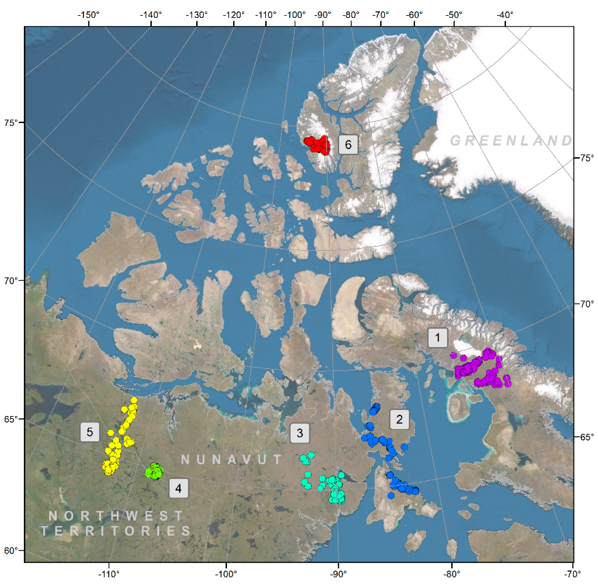
Natural Resources Canada has made considerable efforts to map Canada’s northern geology in the past decades. For example, since 2008, the geo-mapping for energy and minerals was developed to help to unlock the full mineral and energy potential in the North, and to promote responsible land development [34]. Consequently, geological mapping has been conducted in the field by various teams over the years, and abundant gossaneous exposures were identified. However, these gossaneous exposures are currently reported in different maps, reports, and scientific publications. The first step in our study was to identify the location of gossanous deposits in the Canadian Arctic that could be used to train and validate the model. This resulted in the identification of 809 exposures which had the most precise coordinates for our study. These exposures were either reported with coordinates in a publication, consisted of shapefiles in the GEOSCAN database, or they could be easily recognizable in Google Earth Pro or Earth Explorer based on the figures included in each geological report. The 809 gossans used in this study are grouped into six clusters as can be seen in Figure 2. The geological map of the Arctic bedrock compiled by [35] was selected to provide context for our study. This map shows that the gossans from our study can be found on 35 different lithologies. This wide variety of geological contexts is part of the difficulty to identify them. For instance, on the Axel Heiberg Island (cluster 6), most of the gossans are embedded in sandstones, shales, or anhydrites from the Mesozoic era. The gossans from the cluster 5 are mostly in Neoarchean mafic to intermediate volcanic flows and greywackes, some of them related to felsic intrusions. Most of the gossans from the cluster 1 are in metamorphosed siliciclastic rocks dated from the Paleoproterozoic. For more detailed geological settings, please read the description of the geological map from [35].

2.2. Satellite Imagery

Landsat 8 was launched on 11 February 2013. This satellite has 2 instruments called the Operational Land Imager (OLI) and the Thermal Infrared Sensor (TIRS). The OLI acquires data in nine spectral channels between 0.43 and 2.29 µm with a spatial resolution varying between 15 m (panchromatic channel) and 30 m (multispectral channels) per pixel (Table 1). The TIRS acquires data in two spectral channels between 10.60 and 12.51 µm with a spatial resolution of 100 m per pixel. The data acquired by OLI were preferred because of their higher spatial resolution.
All the OLI data used in our study belongs to the United States Geological Survey (USGS) Landsat 8 Surface Reflectance. The process to obtain surface reflectance images from raw data is described in the Landsat 8 Surface Reflectance Code (LASRC) product guide [36]. At high latitude, the atmospheric model used to correct the reflectance could be inappropriate because of high solar zenith angle. Consequently, objects with very high or very low reflectance can be affected and snow results in reflectance values higher than 1. It is a known computational artifact acknowledged by the USGS. Nonetheless, the spectra of other objects like rocks or vegetation seem correct. Landsat 8 was used as the data covered all our areas of study with no cloud and very small amount of snow. In Google Earth Engine (GEE), a script can be written to filter the dates of acquisition for the data. As the region of interest is far North, only images acquired between June 30 and September 30 from 2014 to 2019 were selected to minimize the presence of snow cover. A cloud filter allows to keep only the data with less than 2% of cloud cover. Finally, we chose 6 areas covering the 6 clusters of gossans. The smallest image (cluster 6) covers 9000 km2 and the largest (cluster 2) covers 97,000 km2. To highlight the need of a new method of gossaneous detection in our context, some results were compared with known examples of the literature [3,21]. Hence, we also downloaded OLI imageries of the High lake gossan in Canada and the Khunayqiyah gossans in Saudi Arabia.
A Digital Elevation Model of Canada from GEE provided by Natural Resources Canada [37] was also downloaded. This DEM was derived by integrating various sources of elevation products between 1945 and 2011. The spatial resolution depends on the latitude but is in the same order as the OLI data (~30 m). The vertical resolution varies between 2 and 16 m and is not always known.

2.3. Methodology

CNNs are built in layers, themselves made of neurons. The more the layers, the deeper the network. The training is the iterative adjustment of the weight and the bias for each neuron that minimizes the loss between the predicted output and the given label [38,39]. Each update is called an iteration and an epoch is all the iterations required to see every training samples. The number of epochs can vary depending on the obtained precision. The batch size controls the number of samples “seen” by the model at each iteration before it updates its parameters. The amount of change in the weights and biases at each iteration is called learning rate. In some cases, overfitting can occur during the training, especially with a small training dataset, so the model won’t generalize on new data. A way to prevent overfitting is by adding a dropout layer [40]. This method makes the layers be randomly treated-like layers with a different number of neurons and connectivity to the previous layers. The number of epochs, the learning rate, the batch size, and the probability for the dropout layer are some of the hyperparameters encountered in CNNs. The values for these hyperparameters must be empirically found because they are dependent of the task to be accomplished. Table 2 shows the range of values tested in the frame of our work.
The architecture used in this study, built on pytorch, is inspired from [41]. The latter obtained 95.13% of precision in the classification of the SAT-6 dataset (barren land, trees, grassland, roads, buildings, and water bodies). We chose 2-D convolutional layers with a kernel size of 3 and a stride of 1. Pooling layers lie after the first two convolution layer. After a third convolutional layer, a dropout layer is placed to mitigate overfitting during the training. After the flattening operation, 3 linear fully connected layers were used. The last one has a softmax binary exit for the presence or absence of gossan on the tile, so the output is a number between 0 and 1 for each case. All the other layers have a rectified linear unit (RELU) activation function that outputs directly the input value if positive or 0 if negative. The optimizer is the adaptative moment estimation (Adam) [39] which is a type of stochastic gradient descent algorithm and the loss criterion is the root mean squared error between predictions and labels. The architecture used in our study possesses 93.954 trainable parameters and is shown in the Figure 3.
To detect gossans in a variety of contexts, our goal was to develop a new and effective method involving few steps and a simple CNN architecture. As the quality of the output is dependent of the quality of the input, we decided to test four different datasets as inputs. Here we present the main steps that we undertook, following the method depicted in Figure 3. Our method was tested using iteratively four different datasets as input in the CNN. The first one is the multispectral OLI images converted into reflectance values by the USGS [36]. We kept 7 bands as the cirrus band and the panchromatic band were excluded. The second dataset is the OLI images stacked with the DEM, as gossans are more resistant to erosion if a ferricrete is preserved, than the surrounding terrains. This suggests that a DEM could provide a relevant information to discriminate the presence of gossans. The third dataset is an MNF dataset created from the 7 kept bands of the OLI images in ENVI (Environment for Visualizing Images). A MNF consists of two rotations of principal components analysis [42], which separate the information from the noise. A plot of the eigen values versus the eigen values numbers allows the user to select the number of significant bands that minimize noise and redundant information. Following a visual inspection, we decided to keep the first five MNF bands as the two others were noisy with eigen values close to one. The fourth dataset consists of an MNF dataset created from the OLI images and DEM. In this case, we also kept the first five bands for the same reason. All these data were masked for water and snow areas with ENVI.
To train a CNN, one must construct matrices with their associated labels (presence or absence of gossan). Hence, each OLI image has to be cut in tiles. [43] express how important the context could be to classify a tile extracted from high resolution satellite imagery. This is also discussed in [44] and [31]. The authors explain that a tile should be large enough to give a context to the target, but small enough to not have different objects in it. Gossans can greatly vary in size from a few meters to kilometers. We decided to cut our images in 28 × 28 non-overlapping tiles (840 × 840 m). This area should be large enough to cover a gossan and its immediate surroundings.
When a tile is built from the image, it is considered as positive if a known gossan is either on it or at less than 4 pixels from it. For instance, if a gossan is very close to the border of a tile, the neighboring one could present features corresponding to the presence of a gossan too. Not all the geographical range of the images is cut in tiles because they cover tens of thousands of squared kilometers. As 809 gossans are used, which represents a small fractional area of the OLI images, most of the tiles would be labeled as “negative”. For a balanced training dataset, an equal or nearly equal amount of positive and negative tiles should be identified. To achieve this, each time a positive tile is built, a negative tile is randomly built with no reported gossan on it (or closer than 4 pixels, or 120 m, from the tile). This method raises the question of the false negative tiles. Indeed, a gossan could be present and not being yet detected on a negative tile. We decided to test two approaches. The first approach considers that the chance to have a false negative is small. Indeed, the area covered by the images is large and gossans should be rare enough. Hence, the proportion of false negative in the training dataset should be acceptable and not confusing for the trained model. The second approach decreases the risk of false negative by using a lithological map. For the area of an image, all the known gossans are intersected with their underlying lithology. A histogram is built from the count of the gossans per lithology. Hence, all the negative tiles belonging to the lithology with the highest count are discarded. This should lower the risk of having false negative in the dataset. In the positive dataset, we noticed that gossans being often close to water bodies or sometimes snow, could be associated with no data values (masks). For this case, we also tried two approaches. The first approach considers that these cases occur rarely enough to not confuse the model. The second approach prevents tiles with more than a certain proportion of no data values to be included in the positive dataset. We tried different thresholds for the no data proportion accepted on a tile (25%, 50%, 100%) with and without lithological “filtering”.
The size of the dataset to train a model is of a crucial importance. Indeed, a neural network needs a lot of examples to “learn” the characteristic features of the object and limit overfitting. Different ways are often used to “artificially” increase the amount of data such as cropping, rotating and flipping [45]. In our study, flipped tiles were used (up and down, left, and right) and 180° rotated tiles to multiply by 4 our original dataset. No cropping was done as we thought that tiles of 28 × 28 pixels were already the lower limit.
The normalization is also a commonly used process for the data preparation. To do so, the absolute minimum of the matrix is first added, so there are no more negative values as encountered in MNF images. The matrix is then divided by its maximum value, resulting in a matrix that ranges from 0 to 1. It is then subtracted by its mean and divided by its standard deviation. Hence, the matrix has a mean of 0 and a unit variance.
Our entire dataset contains around 8000 (depending on filters choices) tiles after the augmentation. It is separated in 3 non equal datasets: the training, the validation, and the test datasets. The training dataset that is used to adjust the weights and the biases of the model. The validation dataset is used to evaluate the model between each epoch. The test dataset has never been seen by the model during the training. It allows, at the end of the training, an objective measure of the effectiveness of the obtained model to perform the assigned task. As these data are new to the model, it is equivalent to finding new gossans in unexplored areas never and verifying their presence or absence. It is like having the ground truth data collected before performing the prediction. In our study, we used 10%, 15%, and 20% of all the non-augmented data for the test dataset. The remaining tiles were separated as 80% and 20% for the training and the validation datasets respectively.
To evaluate the model, the precision metric only was used. Indeed, the recall or the F1 score need the false negatives to be accounted. As discussed in the methodology section, the false negatives cannot be identified so their use for evaluation could be misleading. Our method is summarized in the Figure 4.

3. Results

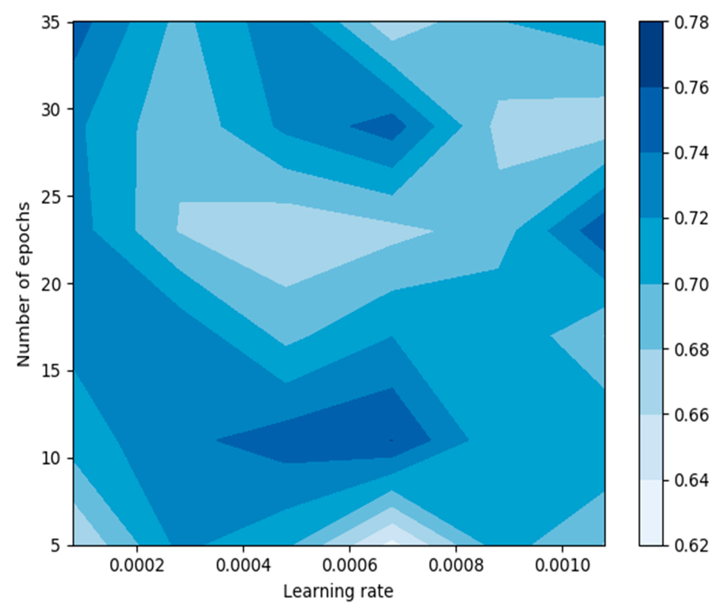
To explore the variability in the predictions based on different model configurations (the 4 datasets with the different filtering conditions), it was necessary to choose a relevant range for the number of epochs and the learning rates. Our trials showed that no significant improvement in the precision of the model could be achieved after ~30 to 40 epochs (Figure 4). For the learning rate, we note that values between 10 × 10−4 and 1.2 × 10⁻³ allowed to get better results (Figure 5). The batch size was set to 64 as greater values decreased precision and smaller values considerably increased the computing time. Consequently, we focus the rest of our analysis on the CNN results obtained using hyperparameter values within these ranges.
The Figure 5 presents an example of a CNN result obtained using hyperparameter values within the ranges mentioned above. This precise example concerns the MNF dataset used as input, without a lithological filter, for a “no data threshold” of 25%, a probability of 0.6 for the dropout layer, and a test dataset representing 10% of the non-augmented data (228 tiles). Indeed, augmented data in our test dataset would have been useless. Figure 6 shows the variability of the precisions, depending on the chosen hyperparameters.
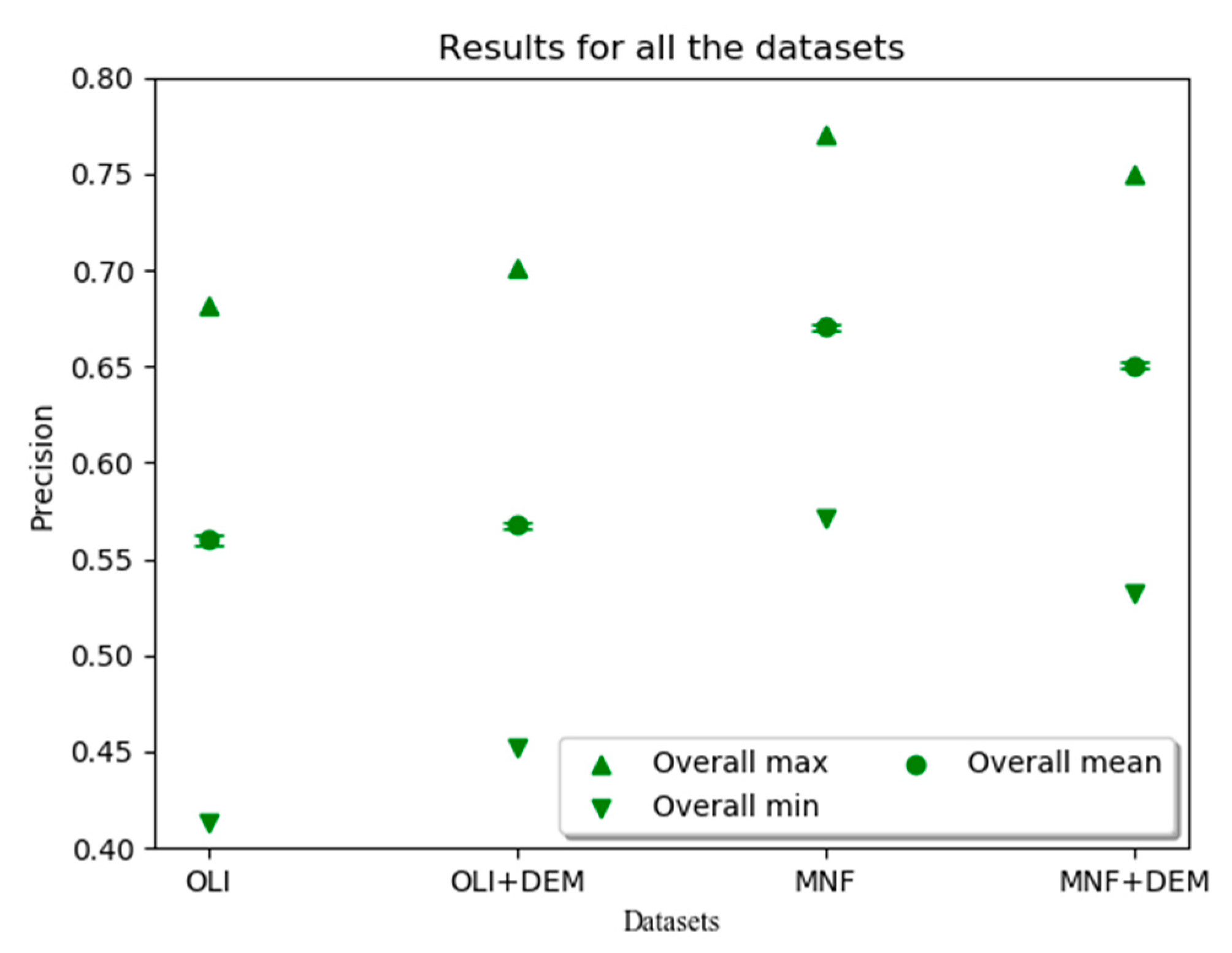
Overall, we produced 288 figures similar to Figure 6 in order to calculate the precisions obtained using each configuration for the datasets. These configurations represent the four different datasets used as input, the six filter configurations (no lithological filter, lithological filter each using no data threshold of 100%, no data threshold of 50%, and no data threshold of 25%), 36 combinations of numbers of epochs and learning rates, three sizes (10%, 15%, and 20% of the non-augmented data) of the test dataset and four values for the dropout layer (0.4, 0.5, 0.6, 0.7). To summarize this information, we present the best and the worst precision obtained for each dataset considering all the different configurations as a whole (Figure 7). This illustrates the variability in the precisions retrieved during the process. Figure 8 shows the same for the six different configurations.

4. Discussion

To detect gossans in the Canadian Arctic, a CNN was trained multiple times with four different datasets (OLI, OLI+DEM, MNF, MNF+DEM) with varying hyperparameters values (number of epochs, learning rates, dropout probabilities).
Figure 7 demonstrates that performing an MNF before training the model, significantly improves the results. Indeed, the best precisions obtained for the OLI and OLI+DEM datasets are respectively 68% and 70%. Concerning the MNF and MNF+DEM datasets, the precisions are 77% and 75% respectively. These results suggest that redundant spatial information may confuse the network. Consequently, further testing could be done with less than five MNF bands used herein. This figure also demonstrates that, contrary as expected, the DEM did not bring relevant information to detect gossans with a CNN. The increase of 2% for the highest precisions in the cases OLI and OLI+DEM should not be considered as significant. Moreover, considering only the mean results for these datasets (56% and 56.8%), the difference is negligible. This could be explained by the resolution of the DEM used, the spatial resolution (30 m), and the vertical resolution (2–16 m) not being enough to detect bumps associated with gossan presence. Still, the experiment should be conducted again with a DEM having a higher resolution.
There is no obvious trend that could be extracted from the tests with different configurations (Figure 8). It seems that no significant change occurs when applying or not a no data threshold. Most of our tiles contain lakes that were masked. We wanted to verify that a model would not associate gossans with no data on a general trend. With no threshold, the number of tiles used in our dataset was 2276. With the lowest threshold (25%), we still could use 1984 tiles. It appears that this difference, 292 tiles representing 13% of the original dataset, was not critical regarding other aspects discussed below. Hence, no influence of the no data has been demonstrated.
The use of a lithological filtering seems to decrease by a few percent the precision of our results. It is not what was expected as the idea was to decrease the risk of false negative in our dataset by avoiding tiles on lithologies associated with gossans. Two reasons to explain this result could be proposed. It is possible that avoiding large areas led to a set of tiles that was not representative of our whole data. Hence, the model could have been confused by a biased negative dataset. It is also possible that this unexpected result came from the way we chose the lithology to avoid. Indeed, we avoided tiles on lithologies where we found the highest count of gossans. We were aware that a bias could arise from this method: the larger the area, the higher the count. This way, we avoided lithologies not necessarily associated with gossans. So, we also tried to normalize these counts by the lithologies areas. Instead of having a gossan count “per lithology”, we obtained a gossan count “per lithology per surface unit”. But a huge artefact arose from this method. Some lithologies were present in small areas in our six clusters. Hence, even with a few gossans on these lithologies, their counts per unit of area were drastically exaggerated. So, this normalization was discarded.
In the literature, it is common to see precisions higher than 90% [31,44] with several classes. What could explain that our best model reached 77% with two classes?
Our first approach to detect the presence of gossans in the Canadian Arctic was using known bands ratios to highlight them. The band ratio the 660/490 nm (B4/B2 with Landsat 8) from [3] and the ratio 1610/865 nm (B6/B5) from [21] were tested. The use of the IFD index from [22,23] was also explored. This index highlights the absorption feature of iron in the near infrared (NIR) band (positive IFD values indicate an absorption). It is calculated by:
I F D = r i n t ( N I R ) r ( N I R )
where I F D denotes the iron feature depth index and r the reflectance. r i n t is the interpolated reflectance calculated by:
r i n t ( 900 n m ) = r ( 750 n m ) + r ( 1250 n m ) r ( 750 n m ) λ ( 900 n m )   λ ( 750 n m ) λ ( 1250 n m ) λ ( 750 n m )
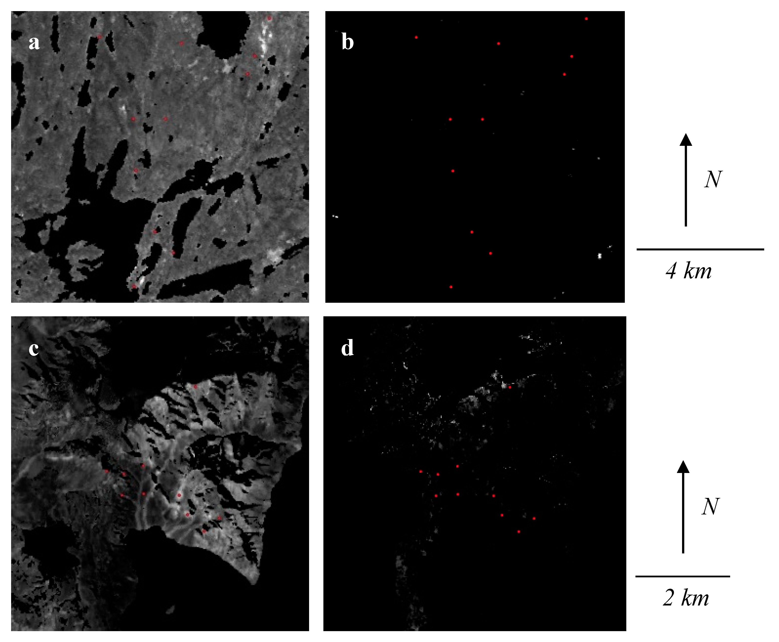
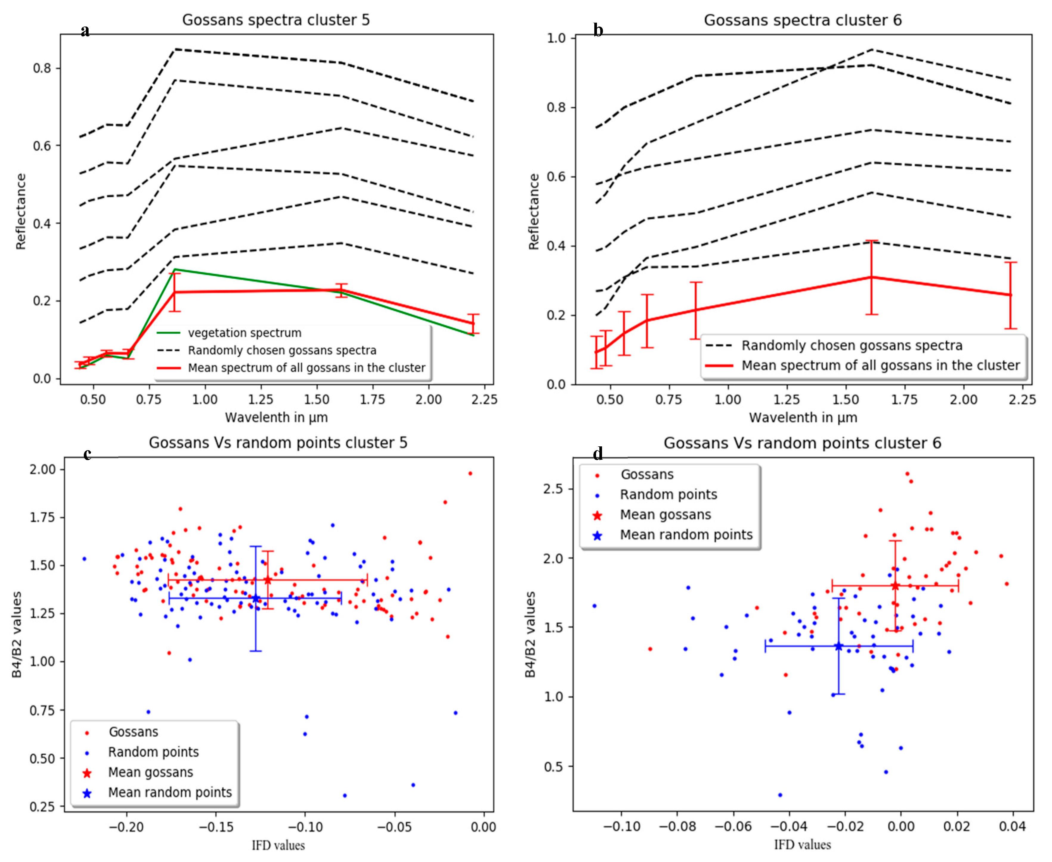
One can see on Figure 9 that these methods are highly effective in the two examples taken from the literature. Gossans are clearly visible on each case, particularly with the IFD index. However, the results on our six clusters are less convincing (Figure 10). Known gossans in our database seem to show no correlation with the band ratio or the IFD. To highlight this observation, we dispatched random points on the images and then extracted their ratio and IFD values. A scatter plot showing B4/B2 versus IFD values allows to compare the repartition of the gossans and the random points in a 2D space. On five of our six clusters, the gossans are undistinguishable from the randomly placed points. Only the cluster six offers a possible separability (Figure 11). Two explanations can be assumed. First, most of our gossans are covered by some vegetation. Second, the occurrences of the gossans are small compared to the spatial resolution, making their spectral contribution in a mixel (not spectrally pure pixel) too small to be detected by these methods. Indeed, spectra of some gossans randomly chosen show that some of them had a vegetation spectrum morphology (Figure 11). Low spatial resolution and vegetation cover could also explain why the band ratioing and the IFD index failed to highlight gossans in our region of study. Hence, the CNN must classify tiles despite showing no apparent spectral common features. Moreover, the non-augmented data represent 2276 tiles only. But training a CNN requires a big amount of labeled data. For a comparison, the SAT-4 dataset has 400,000 images [44]. Also, the tiles from SAT-4 have a high spatial resolution of 1 m per pixel showing detailed features that could be associated with the labels.
As most of the gossans presented in this work do not show recognizable patterns of iron oxides in their reflectance spectra and are undistinguishable from randomly placed points, we think that achieving 77% of precision is a substantial improvement compared to PCA and band ratioing.

5. Conclusions

The remote detection of gossans in the Canadian Artic region to prioritize targets is the utmost importance for different fields of study such as mineralogy, mining exploration, microbiology, or exobiology. In this endeavor, we used satellite imagery from the Landsat 8 sensor OLI and 809 known gossans occurrences to construct labeled tiles (presence or absence of gossan). These data were used to train a convolutional neural network to identify possible presence of a gossan in a tile.
Our work demonstrated that performing a minimum noise fraction before training the model was useful and increased the precision up to 77% on the test dataset (228 tiles). We showed that thresholding the no data proportion on tiles did not improve the precision. Results obtained from the literature were compared with our data. We showed that gossans, assumed as occurrences of yellow and red hues, was too restrictive to apply in our case. For example, a scatter plot of the values of different band ratios for gossans versus random points showed how challenging the detection of gossans could be in our region of study. For these reasons, achieving 77% precision is a success and the method deserves further attention.
The results obtained herein could potentially be refined by modifying the input datasets or the method. For example, higher spatial resolution imagery and digital elevation models could be used as inputs. Such heavy datasets could be processed using tools such as “Google Colab” that offer online GPUs computing capacity. Moreover, hyperspectral imagery is now available in certain regions since the launch of the Precursore Iperspettrale Della Missione Applicativa (PRISMA) mission in 2019 by the Italian Space Agency. This mission provides free hyperspectral imagery, in 237 spectral channels between 400 and 2505 nm, that could provide less redundant information than the OLI dataset for the minimum noise fraction transform used herein and could thus potentially increase the precision of the model. However, the spatial coverage of this dataset is currently limited. In a future study, we propose to use convolutional neural networks and evidential fusion on X data to increase the precision of the model.

Author Contributions

Conceptualization, É.C. and M.L.; methodology, É.C.; M.L. and M.G.; validation, É.C.; M.L.; M.G. and M.-C.W.; formal analysis, É.C.; investigation, É.C.; resources, É.C., M.L.; M.G. and M.-C.W.; data curation, É.C., É.B.; writing—original draft preparation, É.C.; writing—review and editing, É.C.; M.L.; M.G. and M.-C.W.; visualization, É.C., É.B.; supervision, M.L.; project administration, M.L.; funding acquisition, M.L. All authors have read and agreed to the published version of the manuscript.

Funding

This research was undertaken thanks to funding from the Université de Sherbrooke and from the Canada Research Chairs Program. Professor Lemelin is the Canada Research in Northern and Planetary Geological Remote Sensing (950-232175).

Acknowledgments

The authors are grateful to Mathieu Turgeon-Pelchat and the four anonymous reviewers for comments that improved the original manuscript. NRCan contribution no. 20200423.

Conflicts of Interest

The authors declare no conflict of interest. The funders had no role in the design of the study; in the collection, analyses, or interpretation of data; in the writing of the manuscript, or in the decision to publish the results.

References

  1. Velasco, F.; Herrero, J.M.; Suárez, S.; Yusta, I.; Alvaro, A.; Tornos, F. Supergene features and evolution of gossans capping massive sulphide deposits in the Iberian Pyrite Belt. Ore Geol. Rev. 2013, 53, 181–203. [Google Scholar] [CrossRef]
  2. West, L.; McGown, D.J.; Onstott, T.C.; Morris, R.V.; Suchecki, P.; Pratt, L.M. High Lake gossan deposit: An Arctic analogue for ancient Martian surficial processes? Planet. Space Sci. 2009, 57, 1302–1311. [Google Scholar] [CrossRef]
  3. Harris, J.R.; Williamson, M.-C.; Percival, J.B.; Behnia, P.; Macleod, R. Detecting and Mapping Gossans Using Remotely-Sensed Data. In Environmental and Economic Significance of Gossans; Geological Survey of Canada: Ottawa, ON, Canada, 2015; p. 7718. [Google Scholar]
  4. Essalhi, M.; Sizaret, S.; Barbanson, L.; Chen, Y.; Lagroix, F.; Demory, F.; Nieto, J.M.; Sáez, R.; Capitán, M.Á. A case study of the internal structures of gossans and weathering processes in the Iberian Pyrite Belt using magnetic fabrics and paleomagnetic dating. Min. Depos. 2011, 46, 981–999. [Google Scholar] [CrossRef] [Green Version]
  5. Hunt, J.; Lottermoser, B.G.; Parbhakar-Fox, A.; Van Veen, E.; Goemann, K. Precious metals in gossanous waste rocks from the Iberian Pyrite Belt. Miner. Eng. 2016, 87, 45–53. [Google Scholar] [CrossRef]
  6. Peterson, R.C.; Williamson, M.-C.; Rainbird, R.H. Gossan Hill, Victoria Island, Northwest Territories: An analogue for mine waste reactions within permafrost and implication for the subsurface mineralogy of Mars. Earth Planet. Sci. Lett. 2014, 400, 88–93. [Google Scholar] [CrossRef]
  7. Williamson, M.-C. Environmental and Economic Significance of Gossans; Comission Géologique du Canada: Ottawa, ON, Canada, 2015; p. 100. [CrossRef]
  8. Cruz, C.; Noronha, F.; Santos, P.; Mortensen, J.K.; Lima, A. Supergene gold enrichment in the Castromil-Serra da Quinta gold deposit, NW Portugal. Mineral. Mag. 2018, 82, S307–S320. [Google Scholar] [CrossRef]
  9. Valente, T.; Rivera, M.J.; Almeida, S.F.P.; Delgado, C.; Gomes, P.; Grande, J.A.; de la Torre, M.L.; Santisteban, M. Characterization of water reservoirs affected by acid mine drainage: Geochemical, mineralogical, and biological (diatoms) properties of the water. Environ. Sci. Pollut. Res. 2016, 23, 6002–6011. [Google Scholar] [CrossRef] [PubMed]
  10. Santos, E.S.; Abreu, M.M.; Macías, F.; de Varennes, A. Chemical quality of leachates and enzymatic activities in Technosols with gossan and sulfide wastes from the São Domingos mine. J. Soils Sediments 2016, 16, 1366–1382. [Google Scholar] [CrossRef]
  11. Santos, E.S.; Abreu, M.M.; Macías, F.; Magalhães, M.C.F. Potential environmental impact of technosols composed of gossan and sulfide-rich wastes from São Domingos mine: Assay of simulated leaching. J. Soils Sediments 2017, 17, 1369–1383. [Google Scholar] [CrossRef]
  12. Santos, E.S.; Abreu, M.M.; Macías, F. Rehabilitation of mining areas through integrated biotechnological approach: Technosols derived from organic/inorganic wastes and autochthonous plant development. Chemosphere 2019, 224, 765–775. [Google Scholar] [CrossRef]
  13. Shuster, J.; Reith, F.; Izawa, M.; Flemming, R.; Banerjee, N.; Southam, G. Biogeochemical Cycling of Silver in Acidic, Weathering Environments. Minerals 2017, 7, 218. [Google Scholar] [CrossRef]
  14. Hedrich, S.; Schippers, A. Distribution of Acidophilic Microorganisms in Natural and Man-made Acidic Environments. Curr. Issues Mol. Biol. 2020, 25–48. [Google Scholar] [CrossRef] [Green Version]
  15. Floyd, M.A.M.; Williams, A.J.; Grubisic, A.; Emerson, D. Metabolic Processes Preserved as Biosignatures in Iron-Oxidizing Microorganisms: Implications for Biosignature Detection on Mars. Astrobiology 2019, 19, 40–52. [Google Scholar] [CrossRef] [PubMed] [Green Version]
  16. Clark, R.N. Spectroscopy of Rocks and Minerals, and Principles of Spectroscopy. In Manual of Remote Sensing; Remote Sensing for the Earth Sciences; Andrew, N.R., Ed.; John Wiley and Sons: New York, NY, USA, 1999; Volume 3, pp. 3–58. [Google Scholar]
  17. Laakso, K.; Rivard, B.; Rogge, D. Enhanced detection of gossans using hyperspectral data: Example from the Cape Smith Belt of northern Quebec, Canada. ISPRS J. Photogramm. Remote Sens. 2016, 114, 137–150. [Google Scholar] [CrossRef]
  18. Beiranvand Pour, A.; S Park, T.Y.; Park, Y.; Hong, J.K.; M Muslim, A.; Läufer, A.; Crispini, L.; Pradhan, B.; Zoheir, B.; Rahmani, O.; et al. Landsat-8, Advanced Spaceborne Thermal Emission and Reflection Radiometer, and WorldView-3 Multispectral Satellite Imagery for Prospecting Copper-Gold Mineralization in the Northeastern Inglefield Mobile Belt (IMB), Northwest Greenland. Remote Sens. 2019, 11, 2430. [Google Scholar] [CrossRef] [Green Version]
  19. Abrams, M.J.; Ashley, R.P.; Rowan, L.C.; Goetz, A.F.H.; Kahle, A.B. Mapping of hydrothermal alteration in the Cuprite mining district, Nevada, using aircraft scanner images for the spectral region 0.46 to 2.36 µm. Geology 1977, 5, 713–718. [Google Scholar] [CrossRef]
  20. Abrams, M.J.; Brown, D.; Lepley, L.; Sadowski, R. Remote sensing for porphyry copper deposits in southern Arizona. Econ. Geol. 1983, 78, 591–604. [Google Scholar] [CrossRef]
  21. Gahlan, H.; Ghrefat, H. Detection of Gossan Zones in Arid Regions Using Landsat 8 OLI Data: Implication for Mineral Exploration in the Eastern Arabian Shield, Saudi Arabia. Nat. Resour. Res. 2018, 27, 109–124. [Google Scholar] [CrossRef]
  22. Mielke, C.; Muedi, T.; Papenfuss, A.; Boesche, N.K.; Rogass, C.; Gauert, C.D.K.; Altenberger, U.; de Wit, M.J. Multi- and hyperspectral spaceborne remote sensing of the Aggeneys base metal sulphide mineral deposit sites in the Lower Orange River region, South Africa. S. Afr. J. Geol. 2016, 119, 63–76. [Google Scholar] [CrossRef]
  23. Mielke, C.; Boesche, N.; Rogass, C.; Kaufmann, H.; Gauert, C.; de Wit, M. Spaceborne Mine Waste Mineralogy Monitoring in South Africa, Applications for Modern Push-Broom Missions: Hyperion/OLI and EnMAP/Sentinel-2. Remote Sens. 2014, 6, 6790–6816. [Google Scholar] [CrossRef] [Green Version]
  24. Krizhevsky, A.; Sutskever, I.; Hinton, G.E. ImageNet classification with deep convolutional neural networks. Commun. ACM 2017, 60, 84–90. [Google Scholar] [CrossRef]
  25. He, K.; Zhang, X.; Ren, S.; Sun, J. Deep Residual Learning for Image Recognition. In Proceedings of the 2016 IEEE Conference on Computer Vision and Pattern Recognition (CVPR), Las Vegas, NV, USA, 27–30 June 2016; pp. 770–778. [Google Scholar]
  26. Lin, M.; Chen, Q.; Yan, S. Network in Network. Available online: https://arxiv.org/pdf/1312.4400.pdf (accessed on 4 March 2014).
  27. Girshick, R.; Donahue, J.; Darrell, T.; Malik, J. Rich Feature Hierarchies for Accurate Object Detection and Semantic Segmentation. In Proceedings of the 2014 IEEE Conference on Computer Vision and Pattern Recognition, Columbus, OH, USA, 23–28 June 2014; pp. 580–587. [Google Scholar]
  28. Ren, S.; He, K.; Girshick, R.; Sun, J. Faster R-CNN: Towards Real-Time Object Detection with Region Proposal Networks. IEEE Trans. Pattern Anal. Mach. Intell. 2017, 39, 1137–1149. [Google Scholar] [CrossRef] [PubMed] [Green Version]
  29. Dai, J.; He, K.; Sun, J. Instance-Aware Semantic Segmentation via Multi-task Network Cascades. In Proceedings of the 2016 IEEE Conference on Computer Vision and Pattern Recognition (CVPR), Las Vegas, NV, USA, 27–30 June 2016; pp. 3150–3158. [Google Scholar]
  30. Cheng, G.; Yang, C.; Yao, X.; Guo, L.; Han, J. When Deep Learning Meets Metric Learning: Remote Sensing Image Scene Classification via Learning Discriminative CNNs. IEEE Trans. Geosci. Remote Sens. 2018, 56, 2811–2821. [Google Scholar] [CrossRef]
  31. Liu, Q.; Basu, S.; Ganguly, S.; Mukhopadhyay, S.; DiBiano, R.; Karki, M.; Nemani, R. DeepSat V2: Feature augmented convolutional neural nets for satellite image classification. Remote Sens. Lett. 2020, 11, 156–165. [Google Scholar] [CrossRef] [Green Version]
  32. Ducart, D.F.; Silva, A.M.; Toledo, C.L.B.; Assis, L.M. de Mapping iron oxides with Landsat-8/OLI and EO-1/Hyperion imagery from the Serra Norte iron deposits in the Carajás Mineral Province, Brazil. Braz. J. Geol. 2016, 46, 331–349. [Google Scholar] [CrossRef]
  33. Li, S.; Dragicevic, S.; Castro, F.A.; Sester, M.; Winter, S.; Coltekin, A.; Pettit, C.; Jiang, B.; Haworth, J.; Stein, A.; et al. Geospatial big data handling theory and methods: A review and research challenges. ISPRS J. Photogramm. Remote Sens. 2016, 115, 119–133. [Google Scholar] [CrossRef] [Green Version]
  34. GEM: Geo-mapping for Energy and Minerals. Available online: https://www.nrcan.gc.ca/earth-sciences/resources/federal-programs/geomapping-energy-minerals/18215 (accessed on 22 April 2019).
  35. Harrison, J.; St-Onge, M.; Petrov, O.; Strelnikov, S.; Lopatin, B.; Wilson, F.; Tella, S.; Paul, D.; Lynds, T.; Shokalsky, S.; et al. Geological Map of the Arctic; Geological Survey of Canada: Ottawa, ON, Canada, 2011. [CrossRef]
  36. Zanter, K. Landsat 8 Surface Reflectance Code (LASRC) Product Guide; USGS: Sioux Falls, SD, USA, 2019; p. 39.
  37. Canadian Digital Elevation Model, 1945–2011. Available online: https://open.canada.ca/data/en/dataset/7f245e4d-76c2-4caa-951a-45d1d2051333 (accessed on 29 January 2020).
  38. Bottou, L. Large-Scale Machine Learning with Stochastic Gradient Descent. In Proceedings of the COMPSTAT’2010, Paris, France, 22–27 August 2010; Lechevallier, Y., Saporta, G., Eds.; Physica-Verlag HD: Heidelberg, Germany; pp. 177–186. [Google Scholar]
  39. Kingma, D.P.; Ba, J. Adam: A Method for Stochastic Optimization. In Proceedings of the 3rd International Conference on Learning Representations, San Diego, CA, USA, 7–9 May 2015. [Google Scholar]
  40. Srivastava, N.; Hinton, G.; Krizhevsky, A.; Sutskever, I.; Salakhutdinov, R. Dropout: A Simple Way to Prevent Neural Networks from Overfitting. J. Mach. Learn. Res. 2014, 15, 1929–1958. [Google Scholar]
  41. Adivarekar, B. Simple Keras CNN with 95.3% Accuracy. Available online: https://www.kaggle.com/bhumitadivarekar/simple-keras-cnn-with-95-13-accuracy (accessed on 15 January 2020).
  42. Green, A.A.; Berman, M.; Switzer, P.; Craig, M.D. A transformation for ordering multispectral data in terms of image quality with implications for noise removal. IEEE Trans. Geosci. Remote Sens. 1988, 26, 65–74. [Google Scholar] [CrossRef] [Green Version]
  43. Hutchison, D.; Kanade, T.; Kittler, J.; Kleinberg, J.M.; Mattern, F.; Mitchell, J.C.; Naor, M.; Nierstrasz, O.; Pandu Rangan, C.; Steffen, B.; et al. Learning to Detect Roads in High-Resolution Aerial Images. In Computer Vision – ECCV 2010; Daniilidis, K., Maragos, P., Paragios, N., Eds.; Lecture Notes in Computer Science; Springer: Berlin/Heidelberg, Germany, 2010; Volume 6316, pp. 210–223. ISBN 978-3-642-15566-6. [Google Scholar]
  44. Basu, S.; Ganguly, S.; Mukhopadhyay, S.; DiBiano, R.; Karki, M.; Nemani, R. DeepSat: A learning framework for satellite imagery. In Proceedings of the 23rd SIGSPATIAL International Conference on Advances in Geographic Information Systems - GIS ’15, Seattle, WA, USA, 3–6 November 2015; ACM Press: New York, NY, USA; pp. 1–10. [Google Scholar]
  45. Perez, L.; Wang, J. The Effectiveness of Data Augmentation in Image Classification using Deep Learning. Available online: https://arxiv.org/pdf/1712.04621.pdf (accessed on 13 December 2017).
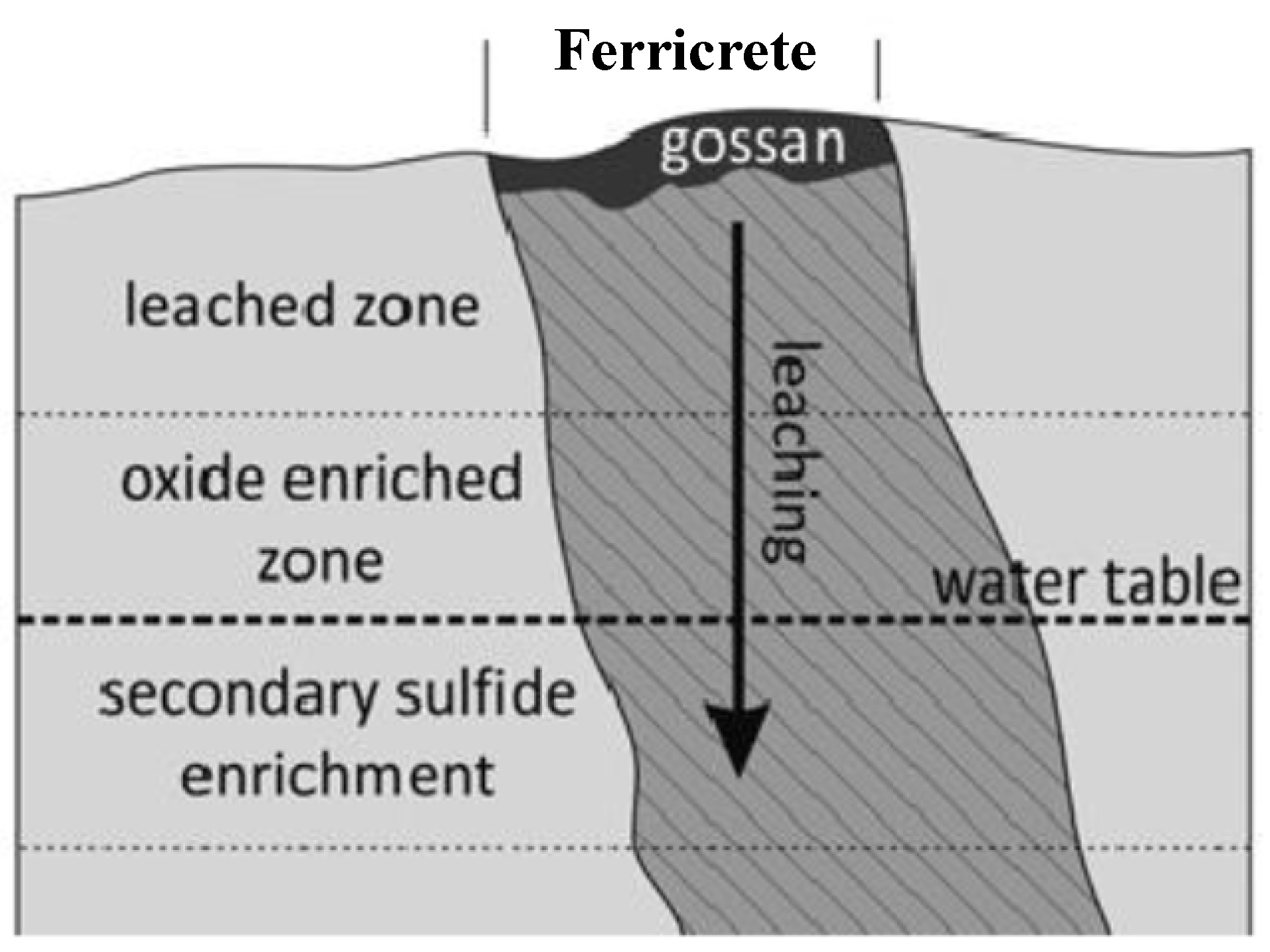
Figure 1. Illustration of a simplified gossan structure adapted from [3].
Remotesensing 12 03123 g001
Figure 2. Location of the gossans used in this study with their associate cluster number to highlight their geographical repartition (colors used for better visualization).
Remotesensing 12 03123 g002
Figure 3. Representation of the convolutional neural network architecture used in this work. This architecture comprises 93.954 training parameters. See main text for details (colors used for better visualization).
Remotesensing 12 03123 g003
Figure 4. Flow chart summarizing the methodology followed in this study.
Remotesensing 12 03123 g004
Figure 5. Variability in the precision of the model using different configurations. (a) When the trained model is applied on the test dataset, one can see that there is no significant improvement in the precision after ~30 to 40 epochs. (b) The same is done while varying the learning rate values. The best results are obtained between 10−4 and 1.2−3.
Remotesensing 12 03123 g005
Figure 6. Example of the overall CNN precisions obtained using number of epochs and lerning rates values within the optimal ranges identified.
Remotesensing 12 03123 g006
Figure 7. Precision obtained for each input dataset considering all the different model configurations as a whole. “Overall max” is the highest precision obtained. “Overall mean” is the mean precision obtained with its standard deviation. “Overall min” is the lowest precision obtained.
Remotesensing 12 03123 g007
Figure 8. Precisions obtained for each input dataset using six different filter configurations. “Overall max” is the highest Precision obtained. “Overall mean” is the mean precision obtained with its standard deviation. “Overall min” is the lowest precision obtained. NLF: no lithological filter, LF: lithological filter, 1: no data threshold 100%, 0.5: no data threshold 50%, 0.25: no data threshold 25%. (a) Precisions obtained on the OLI dataset only. (b) Precisions obtained when the OLI dataset is stacked with a DEM. (c) Precisions obtained on the OLI dataset after using an MNF transform. (d) Precisions obtained on the OLI dataset stacked with a DEM after performing an MNF transform.
Remotesensing 12 03123 g008
Figure 9. B4/B2 band ratio (a) and IFD (b) applied on the Khunayqiyah gossans in Saudi Arabia (long: 45.0794653; lat: 24.2805029). B4/B2 band ratio (c) and IFD (d) applied on the High Lake gossan in Canada (bottom; long: −110.8473047; lat: 67.3826313). The gossans are highlighted by the brightest pixels in both band ratio and IFD.
Remotesensing 12 03123 g009
Figure 10. B4/B2 band ratio (a) and IFD (b) applied on a part of our cluster 5 (top; long: −112.2914268; lat: 66.59684054). B4/B2 band ratio (c) and IFD (d) applied on a part of our cluster 6 (Bottom; long: −93.5884; lat: 79.3667). The red dots represent the known gossans locations. For the band ratio and the IFD, the brightest pixels should have highlighted the gossans.
Remotesensing 12 03123 g010
Figure 11. Mean spectrum of all gossans with 6 randomly chosen spectra for the clusters 5 (a) and 6 (b) (Offset for clarity). Vegetation spectrum added for comparison on the subfigure (a). Scatter plot of IFD values versus band ratio values for the gossans and randomly placed points for the clusters 5 (c) and 6 (d). A slight separation is possible on the latter.
Remotesensing 12 03123 g011
Table 1. Summary of the OLI bands from Landsat 8.
Spectral RangeSpatial Resolution
Band 1 Costal aerosol0.43–0.45 µm30 m
Band 2 Blue0.450–0.51 µm30 m
Band 3 Green0.53–0.59 µm30 m
Band 4 Red0.64–0.67 µm30 m
Band 5 Near-Infrared0.85–0.88 µm30 m
Band 6 SWIR 11.57–1.65 µm30 m
Band 7 SWIR 22.11–2.29 µm30 m
Band 8 Panchromatic0.50–0.68 µm15 m
Band 9 Cirrus1.36–1.38 µm30 m
Table 2. Hyperparameters values tested in the frame of our work.
Min Values TestedKept ValuesMax Values Tested
Number of epochs15–35500
Learning rate10−510−4–10−310−1
Batch size1664256
Dropout probability0.10.4–0.70.9