OLCI A/B Tandem Phase Analysis, Part 3: Post-Tandem Monitoring of Cross-Calibration from Statistics of Deep Convective Clouds Observations

Abstract

This study is a follow-up of a full methodology for the homogenisation and harmonisation of the two Ocean and Land Colour Instrument (OLCI) payloads based on the OLCI-A/OLCI-B tandem phase analysis. This analysis provided cross-calibration factors between the two instruments with a very high precision, providing a ‘truth’ from the direct comparison of simultaneous and collocated acquisitions. The long-term monitoring of such cross-calibration is a prerequisite for an operational application of sensors harmonisation along the mission lifetime, no other tandem phase between OLCI-A and OLCI-B being foreseen due to the cost of such operation. This article presents a novel approach for the monitoring of the OLCI radiometry based on statistics of Deep Convective Clouds (DCC) observations, especially dedicated to accurately monitor the full across-track dependency of the cross-calibration of OLCI-A and OLCI-B. Specifically, the inflexion point of DCC reflectance distributions is used as an indicator of the absolute calibration for each subdivision of the OLCI Field-of-View. This inflexion point is shown to provide better precision than the mode of the distributions which is commonly used in the community. Excess of saturation in OLCI-A high radiances is handled through the analysis of interband relationships between impacted channels and reference channels that are not impacted by saturation. Such analysis also provides efficient insights on the variability of the target’s response as well as on the evolution of the interband calibration of each payload. First, cross-calibration factors obtained over the tandem period allows to develop and validate the approach, notably for the handling of the saturated pixels, based on the comparison with the ‘truth’ obtained from the tandem analysis. Factors obtained out of (and far from) the tandem period then provides evidence that the cross-calibration reported over the tandem period (1–2% bias between the instruments) as well as inter-camera calibration residuals persist with very similar proportions, to the exception of the 400 nm channel and with slightly less precision for the 1020 nm channel. For all OLCI channels, relative differences between the cross-calibration factors obtained from the tandem analysis and the factors obtained over the other period are below 1% from a monthly analysis, even below 0.5% from a multi-monthly analysis). This opens the way not only to an accurate long-term monitoring of the OLCI radiometry but also, and precisely targeted for this study, to the monitoring of the cross-calibration of the two sensors over the mission lifetime. It also provides complementary information to the tandem analysis as the calibration indicators are traced individually for each sensor across-track, confirming and quantifying inter-camera radiometric biases, independently for both sensors. Assumptions used in this study are discussed and validated, also providing a framework for the adaptation of the presented methodology to other optical sensors.

1. Introduction

A meaningful long-term environmental monitoring can only be ensured by the highest quality information. To provide this quality, the Copernicus Space Component (CSC) is continuously provided a fleet of dedicated satellites, the Sentinels, for the retrieval of essential climate variables. Sentinel-3, of the European Space Agency, is one of these satellites [1], providing data continuity for the historical European Remote Sensing (ERS), Environmental Satellite (ENVISAT), and elements of the Project for On-Board Autonomy (PROBA) and Système Probatoire d’Observation de la Terre (SPOT) satellites, owing to state-of-the-art payloads: the Ocean and Land Colour Instrument (OLCI, [2]), the Sea and Land Surface Temperature Radiometer (SLSTR), the SAR Radar Altimeter, and the MicroWave Radiometer (MWR). Sentinel-3 includes two identical satellites flying on-orbit with 140° phase separation to provide global observations daily at the same equator crossing time and meet requirements. At the time of writing Sentinel-3A and Sentinel-3B have been launched and replacement Sentinel-3C and Sentinel-3D satellites are completing their development.

A few weeks after its launch in April 2018, the European Commission Copernicus Sentinel-3B satellite was manoeuvred into a tandem configuration with its identical operational twin Sentinel-3A satellite already in orbit. A dedicated tandem calibration phase was conducted in which both satellites were flown only thirty seconds apart on the same orbit ground track. This approach limits the impact of ocean and atmosphere variability and results in acquisitions over the same targets with the same geometrical conditions. The Sentinel-3A/B tandem phase lasted from early June to mid-October 2018 and provides a unique opportunity to increase knowledge of payload differences, homogenise datasets by defining appropriate adjustments, and to reduce uncertainties when comparing data [3]. It was followed by a short drift phase during which the Sentinel-3B satellite was progressively moved to a specific orbit phasing of 140° separation from the sentinel-3A satellite.

This study bases on the results of a homogenisation and harmonisation methodology for the two OLCI-A and OLCI-B payloads developed through the Sentinel-3 for Climate Study (S3TC), an ESA-funded project (s3tandem.eu), and described in [4]. Homogenisation first adjusts the slight spectral and spatial differences of the two sensors. The comparison of homogenised L1 reflectances acquired during the tandem phase provides evidence of radiometric biases of 1 to 2% between the two sensors, OLCI-A being found brighter than OLCI-B. The quantification of the biases are then used to harmonise the two sensors.

Validation of this harmonisation has been conducted at Level 1 [4] and its full benefits assessed at Levels 2 and 3 for both Land and Water products [5,6]. Among the output of these analyses, the five OLCI cameras have shown residual calibration differences which can be as high as 2%, remarkably consistently between the two payloads. Such residuals cannot be directly monitored from tandem acquisitions.

Cross-comparisons of the two sensors have proven very stable over the tandem period [4]. Throughout the Sentinel-3 mission duration, as no other tandem phase is foreseen, the harmonisation of the sensors would however only rely on the individual in-flight calibration of the two sensors and notably through their temporal stability relating the calibration at the time of acquisition to the calibration at the time of tandem cross-comparisons. As the biases revealed by the tandem configuration were not expected from the in-flight calibration, we have all latitude to think that the root cause of the calibration differences between OLCI-A and OLCI-B may not have the same impact over the mission lifetime. Therefore, it is of high interest to search for a method that could provide the best achievable accuracy in the monitoring of such unexpected calibration differences.

The precision obtained from the tandem phase comparisons (better than 0.5%) is hardly achieved by traditional radiometric validation techniques [7]. However, the precision obtained in the tandem comparisons provide a cross-calibration “truth” against which such traditional techniques can be tested, validated, and eventually improved. This makes the tandem phase dataset a very valuable tool for the calibration/validation community, and presently for our purpose.

We take this opportunity to develop a methodology for the monitoring of the OLCI-A and OLCI-B cross-calibration through statistics of Deep Convective Clouds (DCCs) observations. DCCs are the largest, brightest, and most opaque clouds which can be found on earth’s atmosphere. Their top altitude usually reaches the tropical tropopause (about 16–18 km) which acts as a physical barrier for convection and the formation of water and ice clouds. Tropical convection provides constant formation of DCCs throughout the tropical belt, over land and over water (e.g., [8]), roughly following the slow latitudinal shift of the solar zenith angle across the seasons.

DCCs are widely used for long-term calibration monitoring (e.g., [9,10,11]) and interband monitoring of medium- and high-resolution. optical payloads (e.g., [12,13]), notably owing to the whiteness of their reflectance spectrum from the visible to the near-infrared. The fact that they are white, bright, and opaque provides the best conditions to avoid the propagation of modelling assumptions and associated uncertainties in the analysis as much as possible. We explicitly avoid the use of radiative transfer models to the exception of the modelling of gaseous absorption which is used to convert top-of-atmosphere (TOA) reflectance to gas-corrected ‘DCC reflectance’. This reflectance corresponds to the one that would be measured at top of the cloud, however neglecting slight Rayleigh scattering that could occur. The rationale for using DCC reflectance instead of TOA reflectance is notably to avoid discrepancies between individual acquisitions due to different gas contents. As the approach is statistical, DCC reflectance has more relevance than TOA reflectance.

In a first section, we present the instruments and the selection of the DCC observations, notably from the synergy with SLSTR, a companion S3 payload with thermal channels. Then, the methodology is presented, first by describing gas corrections and the handling of the saturation excess that could damage the analysis, then by presenting the statistical approach along with the metric used to trace the absolute calibration of the instruments.

The across-track (ACT) dependency of the DCC reflectance indicator is exploited to monitor the differences between the two OLCI sensors, benefiting from their similar design and geometry of acquisition as well as the statistical stability of DCC optical properties over the considered sampling period (basically one month). Absolute comparisons are first shown over the tandem duration for verification purpose and proof of concept, and then out of the tandem for a validation of the approach in operational conditions where the two payloads acquire on separate tracks. Comparisons to the tandem reference provides accuracy figures for assessing the performance of the method.

Finally, a sensitivity analysis discusses the assumptions and limitations of the method and provides the requirements to perform this method for future OLCI sensors as well as for other optical sensors.

2. Instruments, Datasets, and Selection of DCC Observations

The selection of DCC observations, among other cloudy targets, relies notably on an estimation of the altitude of the cloud, which can either be obtained from strong absorption features (O₂, H₂O absorption channels) or by thermal information. A common selection criterion of DCC targets employs the 10–12 µm window region brightness temperature [9], an alternative in [12] uses an empirical threshold on the strong water vapour absorption channel at 1375 nm.

Although the objective of this study is focused on OLCI, the provision of 10–12 µm brightness temperature is provided by the synergetic use of SLSTR on-board Sentinel-3, both instruments are briefly described below along with the datasets provision and criteria for the selection of DCC observations.

2.1. Instruments

OLCI [2] is a multi-spectral imaging spectrometer acquiring in the visible (VIS) to near-infrared (NIR) domain (400–1020 nm) dedicated to ocean and land colour science at medium resolution (300 m full resolution, 1.2 km reduced resolution). In the continuity of ESA’s MEdium Resolution Imaging Spectrometer (MERIS), it is a good candidate to become a reference instrument for the radiometry in the VNIR, owing to its advanced on-board calibration devices, wide swath, and medium spectral resolution [2]. More description of the instrument and its calibration are provided in [4], we only recall that OLCI measurements are provided across-track (ACT) owing to the combination of five independent cameras totalizing a field-of-view (FOV) of about 1270 km from a tilted geometry of acquisition covering viewing angles from 46.5° on the west of the FOV to 22.1° on the east.

SLSTR [14] is a high accuracy infrared radiometer inheriting from the previous AATSR and ATSR-1/2 instruments which have flown respectively on Envisat and ERS-1/2 ESA missions. It provides continuity and improvement of these missions with larger swaths (750 km in dual view and 1400 km in single view) allowing a global coverage of sea and land surface temperature measurements with daily revisit, with 1 km spatial resolution in infrared channels. We only make use of the nadir acquisitions of the SLSTR ‘S8’ infrared band at 10.85 µm. These acquisitions cover the entire OLCI FOV, resulting in no observation gaps and complementarity for the analysis of OLCI measurements.

2.2. Datasets

As in [4], the tandem phase datasets used in this work were collected in the frame of the Sentinel-3 Tandem for Climate project. The project data archive contains Sentinel-3A and Sentinel-3B data for all instruments, collected one day per week (Monday) between 25 June 2018 and 18 March 2019. This includes tandem (6 June 2018 to 15 October 2018), drift (22 October 2018 to 19 November 2018) and post-tandem phases. More details on the project can be found in [4]. These ‘baseline’ products were collected from the Payload Data Ground Segment (PDGS, Land and Marine centres). For our purpose, we use OLCI L1B Full Resolution (FR) products from which the harmonisation methodology in [4] has been developed. SLSTR S8 brightness temperatures (BT) are provided from the L1 products available over the same period. We only make use of tandem data from this archive.

More recent data are taken from the rolling archive of the Sentinel-3 Mission Performance Centre [15], it covers the months of November 2019 as well as January, March, and May 2020. Preliminary choice has indeed been made to analyse one month over two.

None of these datasets are provided with the radiometric alignment of OLCI-A and OLCI-B performed in [4] as the objective of this work is to assess the ability to retrieve the cross-calibration information extracted from the tandem analysis but, in fine, without the use of the tandem configuration. All OLCI and SLSTR acquisitions are taken at Full Resolution (FR), it is however convenient to consider blocks of 20 × 20 pixels (in the following called ‘macropixels’) instead of individual pixels, all the more as it facilitates the handling of a very large volume of data.

2.3. Data Preparation, Selection of DCC Observations, Saturation Tagging

OLCI L1 radiances and SLSTR L1 BT products are subdivided into granules, elements of orbits corresponding to three minutes of acquisition (about 1000 km along-track). As in [4], it is most useful and relevant to reproject acquisitions over the same grid prior analysis (see [4] for details), discarding pixels for which any considered sensor is missing. This reprojection is performed similarly for all useful parameters, owing to the L1B geolocation information: radiance measurements, auxiliary data (ozone content, solar irradiance, geometry of acquisition, detector indices).

For tandem phase products, OLCI-A, OLCI-B, and SLSTR-A are coregistered through such reprojection. Out of tandem, OLCI-A and SLSTR-A (resp. OLCI-B and SLSTR-B) are coregistered similarly, individually per pair of Sentinel-3 instruments as the Sentinel-3A and Sentinel-3B platforms are on separated orbital tracks.

The selection of pixels containing DCCs is first performed on the tropical band 25 °N–25 °S, not excluding any geographical region, with BT < 225 K, which leaves ability for post-processing selection and sensitivity analysis. Example of a beautiful DCC, acquired on 3 September 2018 (OLCI-A granule ‘20180903T081702_20180903T082002’), is shown in Figure 1 with OLCI-A top-of-atmosphere (TOA) reflectance at 412 nm on the left and SLSTR 10.85 µm BT on the right. This DCC covers a circular area whose diameter is about 200 km, overshooting convection (left-hand side of the cloud with lowest BTs) and wide cirrus anvil (most of the cloud) appear nicely. It is striking to see the structural effects triggered by overshooting, progressively smoothed out as we progress out of the convection core. The corresponding reflectance is much more dispersed over the overshooting area where three-dimensional effects provide values as different as between 0.5 and 1.2.

DCCs are among the brightest targets on earth, as shown above it is not uncommon to spot reflectance higher than unity induced by optical effects. Consequently, saturation may occur at detector level when the input radiance exceeds the energy flux allowed by the detector sensitivity. It is worth mentioning that such radiance levels can be considered for optical sensors as upper limits for the dynamic range allowed in sensors design.

In OLCI, most differences in the sensitivity to high radiances are found between the spectral bands as each band is designed with a sensitivity that depends on its dedicated application. One reference band is considered at 412 nm (band Oa02) where saturation very seldom occurs.

Saturation shows up with very abnormal values (see Figure 2) which are traced within the OLCI processing chain from raw data packets up to the next levels.

Figure 2 highlights the difference between OLCI-A and OLCI-B, the latter being much less affected by saturation. Indeed, a statistics of the saturated pixels is provided below in Figure 3 per spectral channel and detector index from a large number of DCC observations for OLCI-A (left) and OLCI-B (right).

The figures obtained for OLCI-B are relevant to the expectation of the mission design: all bands seldom saturate to the exception of the bands with strongest absorption (Oa14 for O₂ and Oa20 for H₂O) which are designed to be sensitive to absorption in clear atmospheres. Compared to OLCI-B, OLCI-A shows a much larger rate of saturated pixels, which can somehow be related to the fact that OLCI-A is brighter than OLCI-B, corroborating that the difference in radiometry is independent of the detecting unit (coupled charge devices in this case) and is rather unexpected. The eastern part of the FOV is also more prone to saturation as the geometrical configuration is that of sun reflecting more directly at the clouds surface, providing higher reflected radiance, camera 1 (on the left-hand side) is the least affected.

The relatively high saturation occurrence of OLCI-A is a major constraint for an accurate monitoring of its calibration using DCC observations. To overcome this issue, we base on the whiteness of DCCs to reconstruct the saturated pixels from the interband relationships (i.e., the ratio of the reflectance) between the bands impacted by saturation and its closest reference channel(s). Reference channels are taken as those least affected by saturation, i.e., Oa01 (412 nm), Oa06 (560 nm), Oa09 (674 nm), Oa18 (885 nm), and Oa19 (900 nm).

When DCC pixels are selected from their original context and tagged with respect to saturation, a very large database is gathered from which our methodology is deployed as presented in the next section.

3. Methodology

Our methodology is based on the exploitation of the DCC reflectance statistics from OLCI-A and OLCI-B individually. Solar irradiance and gaseous absorption correction are first performed to convert the L1 TOA radiance products into gaseous-corrected reflectance, interband relationships are found between bands affected by saturation and reference bands for an empirical correction of the saturated measurements.

Then, reflectance statistics are performed keeping the ACT dependency of the sampling. Whereas most methods using DCC observations exploit the mode of the corresponding probability distributions, we propose a novel approach by exploiting the position of the maximum gradient (an inflexion point), which is shown to provide better precision in this context.

3.1. Conversion of TOA Radiances Into Gas-Corrected Reflectances

The next step in preparing the data consists in first converting TOA radiances into TOA reflectances and then in handling the two-way gaseous transmission to correct the TOA reflectances for the gaseous absorption occurring above the clouds.

As in [4], the radiance-to-reflectance conversion handles the normalisation of the upcoming radiance arising from the target to the sensor by the incoming solar illumination received by the target and convolved with the instrument spectral response function. In the radiance-to-reflectance formulation the radiance $L\left(\lambda \right)$ is converted to the reflectance $\rho \left(\lambda \right)$ through

$$\rho \left(\lambda \right)=\frac{\pi L\left(\lambda \right)d^2}{F_0\left(\lambda \right)\cos {\theta }_s}$$

(1)

The solar illumination $F_0\left(\lambda \right)$ is scaled by the solar zenith angle ${\theta }_s$ seen by the target (0° corresponding to maximum illumination with Sun at zenith) and $d^2$ the Earth–Sun distance in astronomical units. $F_0\left(\lambda \right)$ is taken from Thuillier [16] and its convolution with the instrument spectral response function (ISRF) is performed from the spectral characterisation per detector and included in each L1B product. The conversion to reflectance is coherent with the absolute calibration methodology which uses a reflectance reference.

The gaseous correction is performed in a way similar as in [12]: radiative transfer simulations are performed within the ARTDECO (Atmospheric Radiative Transfer Database for Earth and Climate Observation) framework (http://www.icare.univ-lille1.fr/projects/artdeco). Gaseous transmissions are simulated every 1 nm across the complete OLCI spectrum using the standard tropical atmosphere profile of McClatchey [17] between TOA and a cloud whose top altitude is taken at 16 km to represent a mean DCC. H₂O, NO₂, O₃, and O₂ are considered as these are the most absorbing gases within the OLCI channels. Simulations are tabulated for various ozone contents for interpolation by the actual ozone content delivered in the OLCI product (originally provided by reanalyses from the European Centre for Medium-Range Weather Forecasts). Indeed, ozone variability must be taken into account to remove its varying impact on TOA reflectance, which may bring noise and/or bias in a statistical approach. The correction of the absorption from the other gases has no real impact as a typical DCC scenario and a similar tropical atmospheric profile are considered for all acquisitions, these are provided for the sake of completeness. However, H₂O and O₂ absorption corrections at (very) high spectral resolution would benefit for channels impacted by smile over strong absorption spectral regions.

The nadir-zenith two-way transmission at wavelength $\lambda$ $T_{gas}\left(0, 0, \lambda \right)$ is converted to the transmission in the geometry of acquisition $T_{gas}\left({\theta }_s,{\theta }_v,\lambda \right)$ using the total airmass $m$ as:

$$T_{gas}\left({\theta }_s,{\theta }_v,\lambda \right)=T_{gas}{\left(0, 0, \lambda \right)}^{m/2}$$

(2)

$$m=\frac{1}{\cos {\theta }_s}+\frac{1}{\cos {\theta }_v}$$

(3)

where ${\theta }_s$ and ${\theta }_v$ are respectively the illumination and viewing zenith angles. Then the gaseous-corrected reflectance ${\rho }_{DCC}$ is derived from the TOA reflectance ${\rho }_{TOA}$ as

$${\rho }_{DCC}\left({\theta }_s,{\theta }_v,{\mathsf{\Delta }}_{\phi },\lambda \right)=\frac{{\rho }_{TOA}\left({\theta }_s,{\theta }_v,\mathsf{\Delta }\phi ,\lambda \right)}{T_{gas}\left({\theta }_s,{\theta }_v,\lambda \right)}$$

(4)

The resulting spectrum is the one of a DCC, possibly with slight Rayleigh scattering residuals in the blue part of the spectrum as well as slight uncertainties in the estimation of ozone absorption as the top of the cloud is fixed average at 16 km whereas it can take various values in reality. As we shall see, this will not impact the analysis.

3.2. DCC Interband Statistics, Reconstruction of Saturated Pixels

In this study, we do not intend to investigate the spectral consistency of the OLCI calibration, although it could be performed similarly as in [9] by comparing the shape of DCC reflectance spectra against reference spectra from cloud models. Interband relationships however provide very valuable information in our context, first to empirically correct saturated pixels, and second to detect slight calibration residuals, specific to some channels, which can only be apprehended by comparisons between channels over a white and bright target.

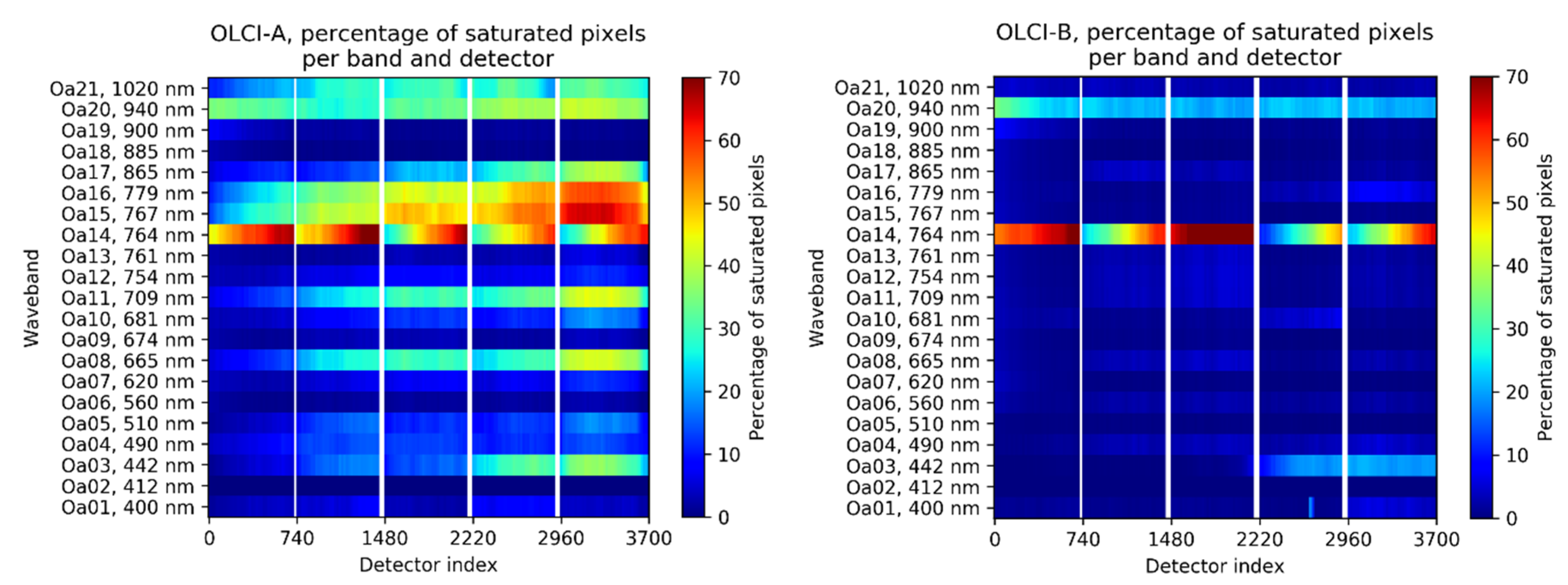
As most OLCI channels are affected by saturation, the idea is first to compute the mean interband relationships against the reference channels Oa02, Oa06, Oa09, Oa18, and Oa19 from the measurements that are not affected by saturation, statistics being computed between each channel and the closest reference channel. Interband relationships $I\left(\lambda ,{\lambda }_{ref}\right)$ then simply consist in the ratios between the two reflectances as:

$$I\left(\lambda ,{\lambda }_{ref}\right)=\frac{{\rho }_{DCC}\left(\lambda \right)}{{\rho }_{DCC}\left({\lambda }_{ref}\right)}$$

(5)

Then, assuming that the interband relationships hold for the saturated pixels, the reflectance from the affected channel is reconstructed from the one of the reference channel and the interband relationship. As we shall see, $I\left(\lambda ,{\lambda }_{ref}\right)$ is also found depending on the reference reflectance and will be further apprehended through a polynomial formulation of this reflectance.

Table 1. OLCI band affected by saturation and reference band used for the computation of interband relationships over DCCs, spectral distance added for information. Oa01 (400 nm) to Oa12 (753.75 nm). OLCI band affected by saturation and reference band used for the computation of interband relationships over DCCs, spectral distance added for information. Oa13 (761.25 nm) to Oa21 (1020 nm).

Band (nm)	Oa01 (400)	Oa03 (442.5)	Oa04 (490)	Oa05 (510)	Oa07 (620)	Oa08 (665)	Oa10 (681.25)	Oa11 (708.75)	Oa12 (753.75)	Oa13 (761.25)	Oa14 (764.375)	Oa15 (767.5)	Oa16 (778.75)		Oa17 (865)	Oa20 (940)	Oa21 (1020)
Reference (nm)	Oa02 (412.5)	Oa02 (412.5)	Oa06 (560)	Oa06 (560)	Oa06 (560)	Oa09 (673.75)	Oa09 (673.75)	Oa09 (673.75)	Oa09 (673.75)	Oa09 (673.75)	Oa09 (673.75)	Oa09 (673.75)	Oa09 (673.75)	Oa18 (885)	Oa18 (885)	Oa18 (885)	Oa18 (885)
Spectral distance	−12.5	30	−70	−50	60	−8.75	7.5	45	80	87.5	90.625	93.75	105	−106.25	−20	55	135

first recaps the correspondence between the OLCI channels affected by saturation and the closest reference channel(s) used for the saturated reflectance reconstruction. As Oa16 (779 nm) lies between Oa09 (674 nm) and Oa18 (885 nm), interband relationships are sought against those two channels independently. For Oa20 and Oa21, we choose Oa18 (885 nm) as the reference instead of Oa19 (900 nm) as the latter is impacted by water vapour absorption (although much attenuated considering DCC altitude and opacity) and the interband relationships gets slightly less precise (not shown). Spectral distance is also mentioned, the larger this latter is the noisier may be the interband relationship. Indeed, in [9] larger discrepancies were found in such relationships for channels farther from the considered reference channel.

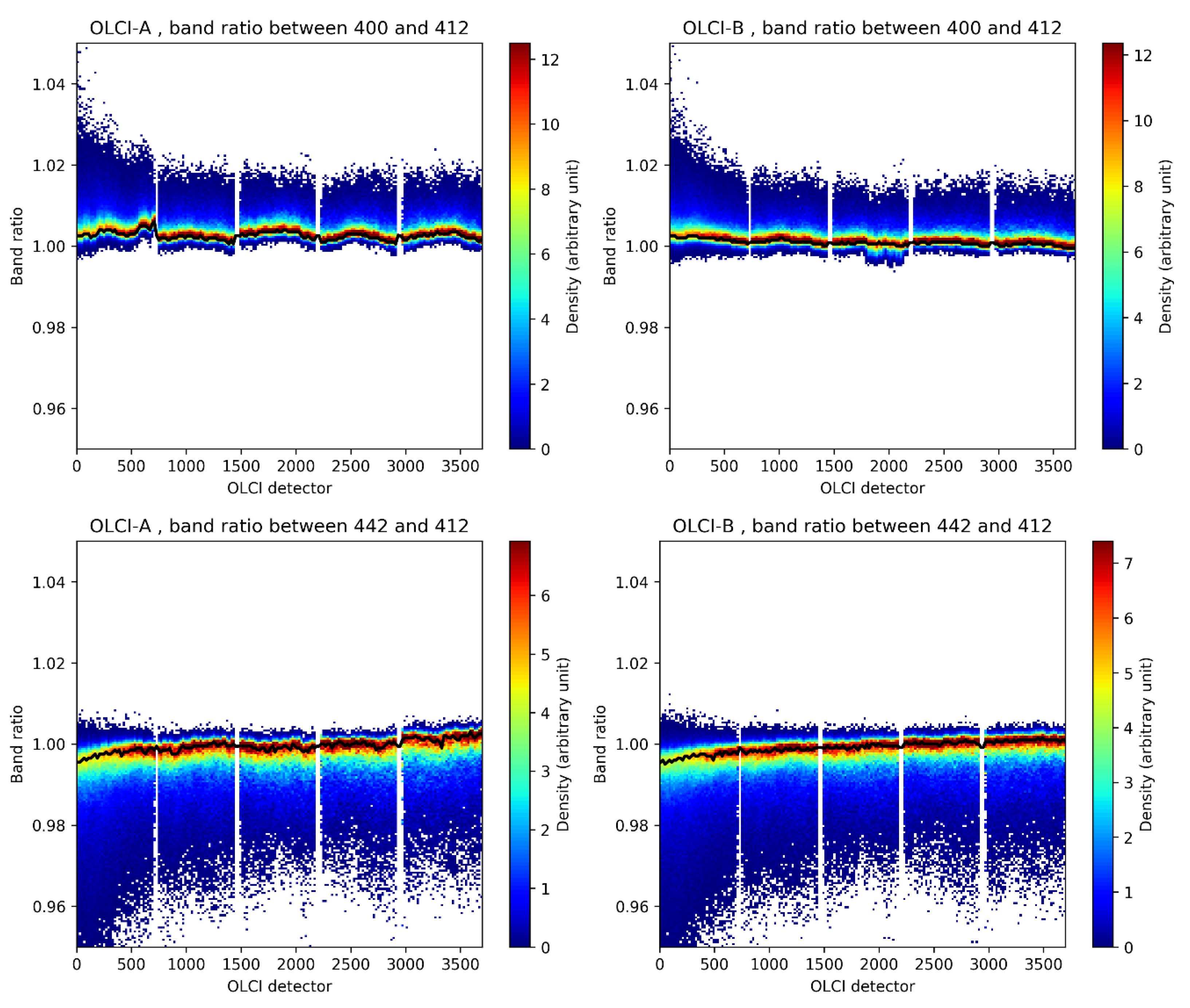
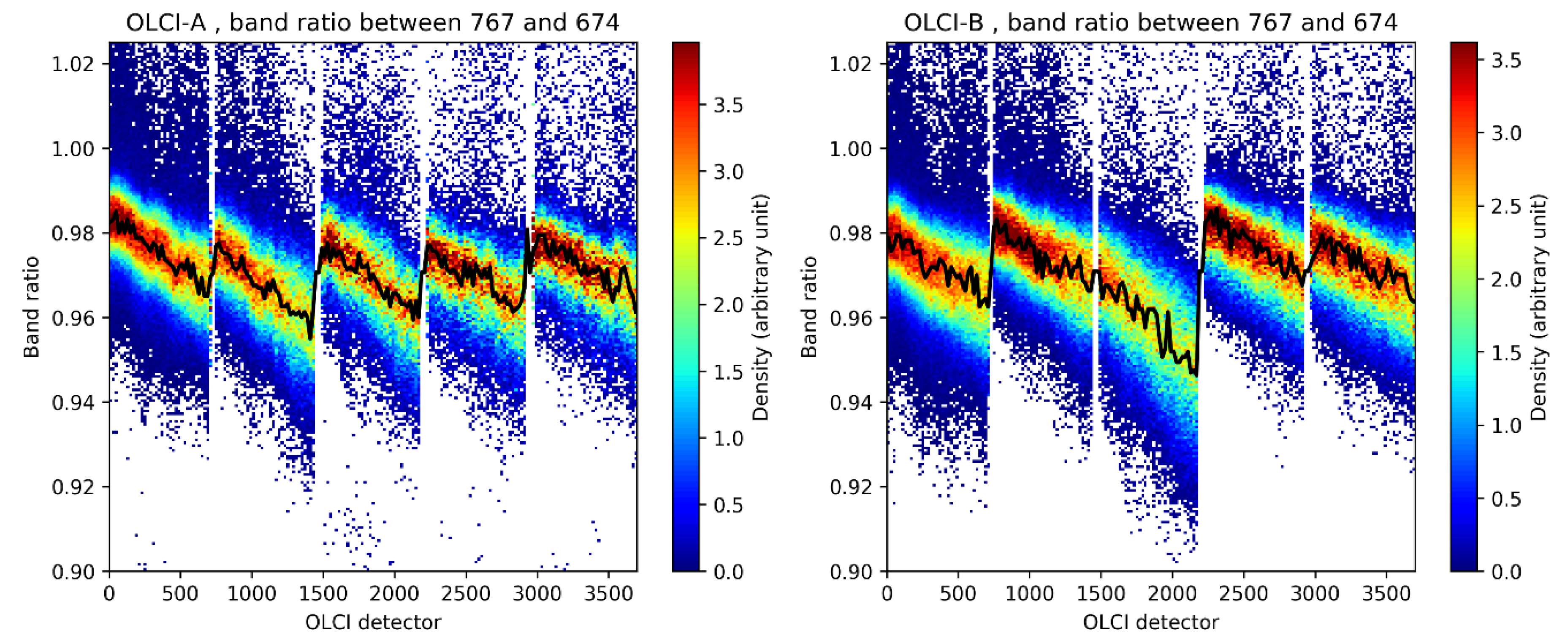
Density plots of $I\left(\lambda ,{\lambda }_{ref}\right)$ are first displayed in Figure 4 and Figure 5 from statistics over the tandem phase dataset, individually for OLCI-A (left) and OLCI-B (right). Black lines indicate the median in each OLCI detector bin. Between cameras, gaps stand for the detector indices that correspond to measurements made by two adjacent cameras and which are not used in the nominal products, the average relationship is however used to fill the gaps visually. Completing results are displayed in Supplement Figures S1 to S3 showing very stable interband relationships ACT both for OLCI-A and OLCI-B.

As the sampled DCCs, by nature, exhibit microphysical and macrophysical variability, variability in their reflectance spectrum produces noise in these figures, whose amplitude qualitatively depends on the spectral distance between the two considered wavebands.

Results for Oa01 (400 nm) in Figure 4 exhibit an unexpected behaviour (broken lines) for OLCI-A on the right-hand side of camera 1 (detector indices approximately between 550 and 740). Such behaviour can be distinguished in the tandem comparisons [4], Figure 8, and has not been considered in the computation of the cross-calibration factors aligning OLCI-A and OLCI-B, the present figure proves that it is caused only by a calibration residual in the OLCI-A radiometry. As Oa03 (442 nm) also uses Oa02 (412 nm) as reference, we see that there is no such behaviour between Oa03 and Oa02 which consequently confirms that it is not related to measurements in Oa02.

Variability ACT is found in the interband between Oa03 and Oa02 (about 0.995 on the left-hand side, about 1.0 on the right-hand side), which is possibly related to residual Rayleigh scattering above the cloud, correlated with the airmass (much larger for camera 1), and accentuated by the spectral distance between the two bands (30 nm between Oa03 and Oa02 against 12 nm between Oa01 and Oa02 where such discrepancies may also appear). This residual Rayleigh may also be responsible of additional asymmetrical noise in the interband relationships in the blue-green region (depending on the position of the considered band against the reference, this noise tends to be more pronounced on one or the other side of the mean relationship).

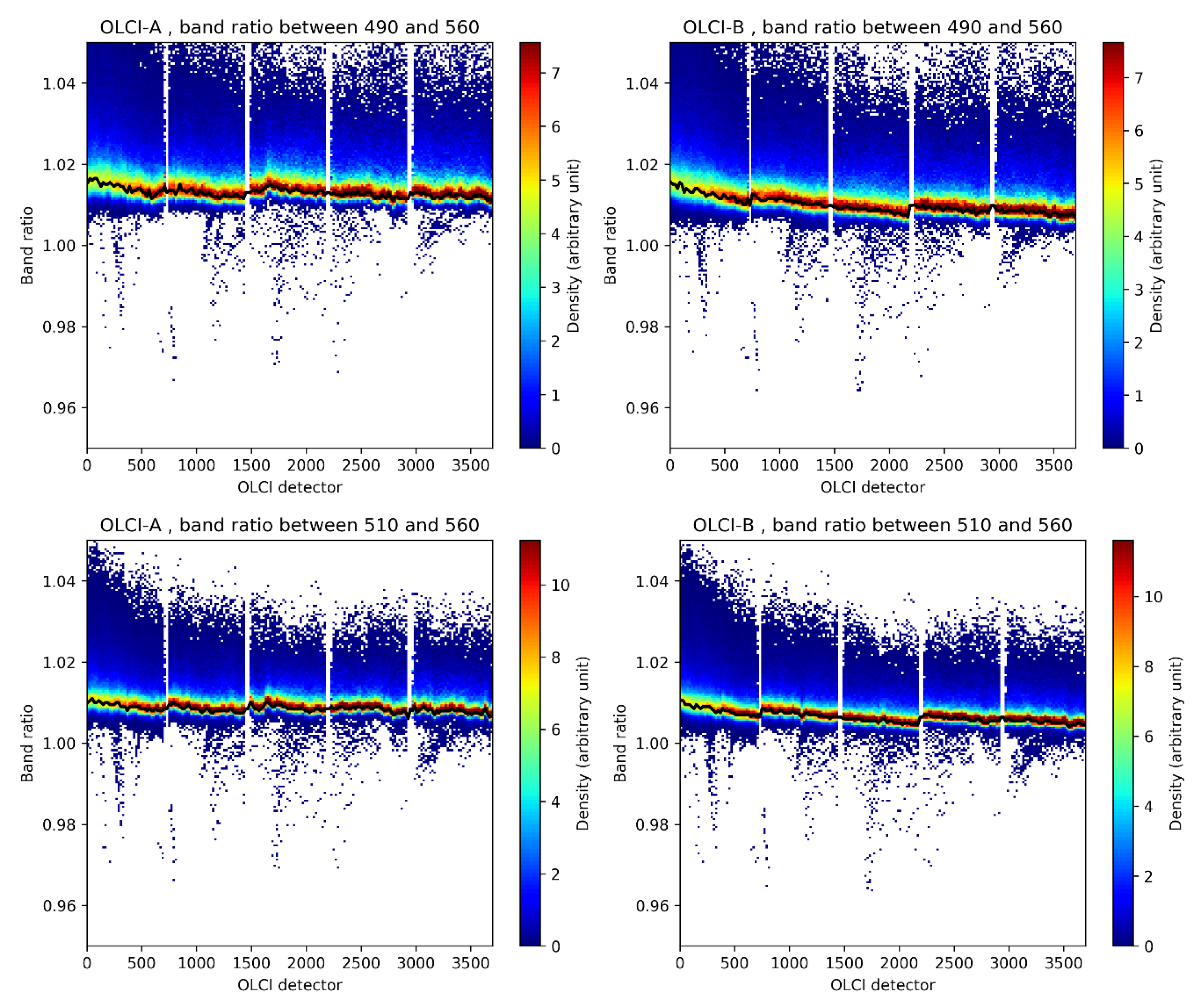
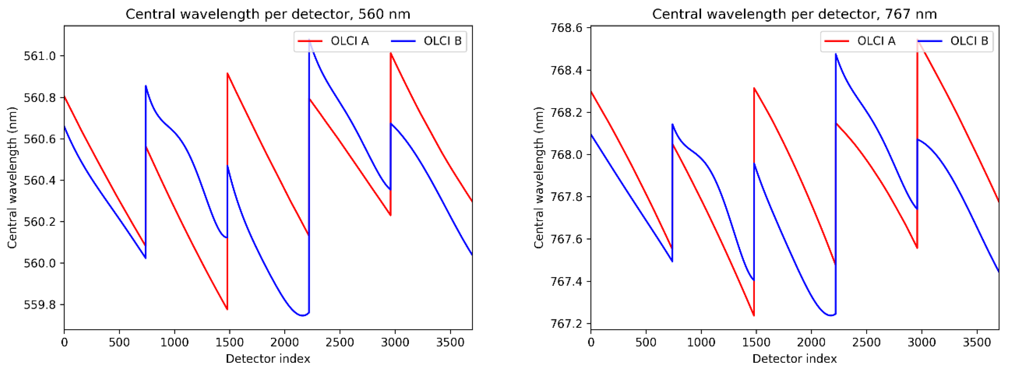
Between Oa04 (490 nm) or Oa05 (510 nm) and their same reference Oa06 (560 nm) in Figure 5 we see broken lines at camera interfaces which are most probably due to the handling of ozone absorption originally performed at a spectral resolution of 1 nm, which is insufficient to resolve tiny variations of the absorption due to spectral smile (i.e., the variability of the wavelength of acquisition through a camera FOV) as shown in Figure 6 for Oa06 (left) and Oa15 (right, see rationale below). It is indeed interesting to see that a visual continuity of the spectral characterisation of OLCI-B (contrary to OLCI-A) occurs between cameras 2 and 3 as well as between cameras 4 and 5, corresponding to the continuity of the interband relationships between the same cameras and in Figure 5.

Another drawback of having a relatively coarse spectral resolution in the gaseous transmission computation is the inability to account for strong and fine absorption lines, which is necessary to convert TOA reflectance to DCC reflectance in the specific O₂ and H₂O (water vapour) absorption bands Oa14, Oa15, Oa16, and Oa20. Would high spectral resolution be achieved, the knowledge of O₂ and H₂O content above (and within) the top of the cloud however requires an accurate knowledge of the cloud altitude and its opacity as well as of the actual O₂ and H₂O contents that effectively absorb. Nevertheless, the interband relationships between an absorption band and a reference, not absorbing, band allows, for Oa15 where absorption is relatively weaker (see Figure 7), to spot intra-camera variability coherent with the spectral characterisation of OLCI, which proves the correlation between the spectral position in the absorbing region and the TOA reflectance. Indeed, the DCC reflectance being presently corrected for absorption at low spectral resolution, we can reasonably extrapolate the relationships in Figure 7 to TOA reflectance. Remarkably, OLCI-B does not behave similarly as OLCI-A in camera 3, which is not coherent with its spectral characterisation as shown in Figure 6 (right). This shows the potential of using measurements over DCCs to highlight spectral issues in such bands.

Last but not least, the relationships found between the band Oa21 (1020 nm) and the reference band Oa18 (885 nm) highlight two unexpected behaviours in Figure 8: first, strong variability is found in the distributions of the interband ratios; second, OLCI-A and OLCI-B do not behave similarly although over the tandem phase the sampled targets can be considered similar thirty seconds apart.

This is due to the combination of two facts: first, the sampling of non-saturated reflectance is limited in OLCI-A compared to OLCI-B; second, there is strong variability of the interband ratio with the level of reflectance (here roughly between 0.85 and 1.0). Such variability can be apprehended through comparing the interband ratio to the reference reflectance and to brightness temperature in Figure 9.

Clearly, there is a smooth, yet strong, variation of the ratio against the reference reflectance which is cut at lower values for OLCI-A than for OLCI-B due to saturation in OLCI-A. The variation against temperature also shows that two regimes of the ratio appears for either “cold” (below 205 K) or “warm” (above 210 K) temperatures, possibly related to the optical response of different microphysical and macrophysical composition of the DCC targets.

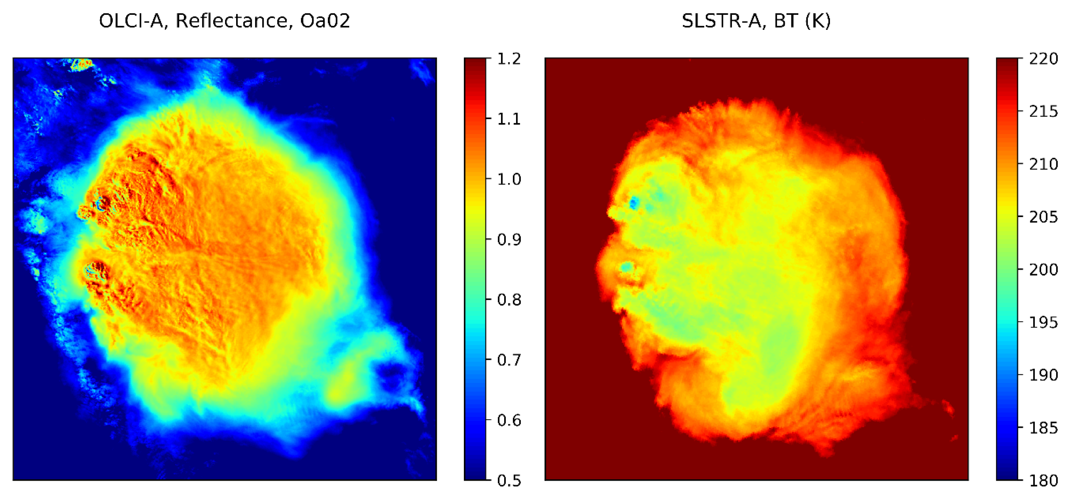
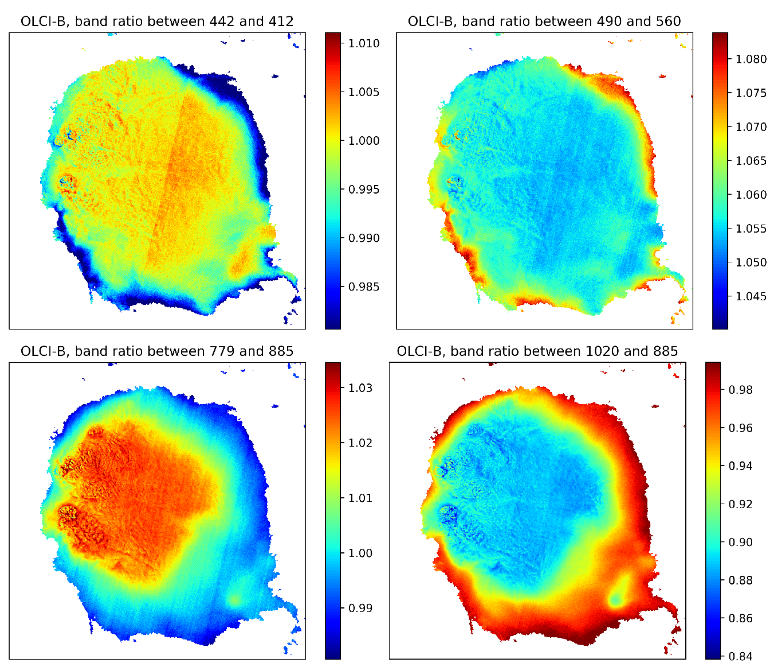
To this respect, the mapping of such interband ratios computed over the observation case presented in Figure 1 is most instructive (below in Figure 10 for OLCI-B only). Indeed, such observation case provides an example of a DCC with a large convection core (on the left of the cloud with two overshooting tops), and a warmer large cirrus anvil spread all around the core and slightly more on the right-hand side. It is assumed that the cloud microphysical and macrophysical compositions varies much from the core to the outside within the cirrus anvil. Two examples in the VIS (Oa03 and Oa04, resp. 442 and 490 nm), and two examples in the NIR (Oa16 and Oa21, resp. 779 and 1020 nm) are presented. Note that a camera interface can be spotted as the cloud is located right within the footprint of two adjacent cameras.

In the VIS, it appears clearly that the interband ratios are only slightly dependent of the position (and composition) in the cloud. Rather, stronger boundary effects appear at the border of the cloud, which are representative of what causes the noise sampled in Figure 4 and Figure 5.

In the NIR, there are stronger differences according to the position in the cloud and hence to temperature (see again Figure 1 for BT map) as reported in Figure 9.

The expression of the interband ratios against the reference reflectance is found smoother and less noisy than the expression against the position in the OLCI FOV. All channels exhibit such variability, however stronger for NIR channels (see Supplementary Figures S4 to S7). This provides a very convenient and necessary way to handle the variability of the ratios corresponding to various cloud compositions.

For most channels, the relationship is smooth enough to relate the missing saturated reflectance values to the continuity of a polynomial fit as computed and represented in the figures. For the NIR bands Oa16 (779 nm) and Oa21 (shown above), the relationships are too affected by missing reflectance values for OLCI-A, which is to be compared to the relationships found for OLCI-B. Consequently, the relationships found for OLCI-B are considered for use in OLCI-A for reconstructing the saturated reflectance of these two bands. This is made possible because of the spectral and radiometric consistency between OLCI-A and OLCI-B, however, very slight differences may bring a lack of precision, especially for Oa21 as the end of the distributions (excluding the unavailable saturated values for OLCI-A) in Figure 9 seem slightly different.

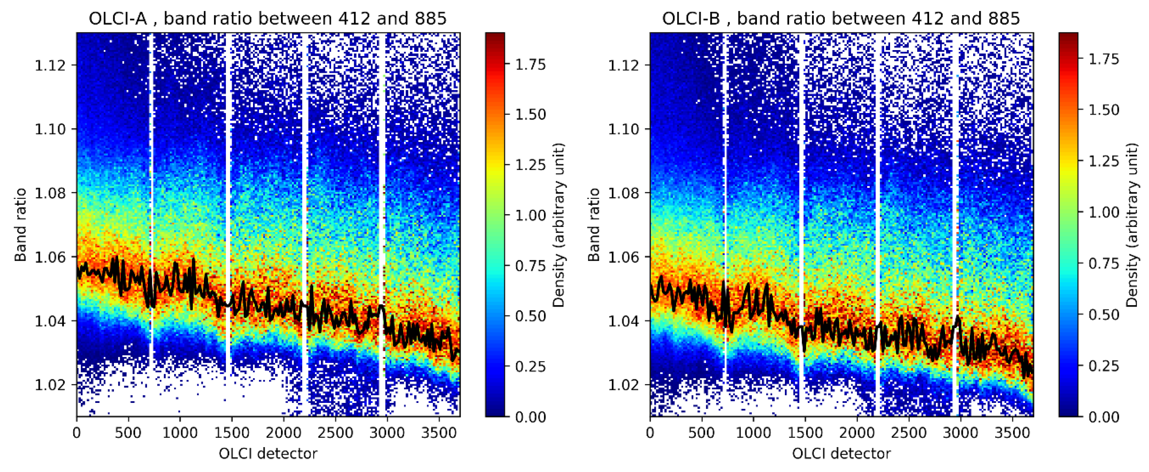
For information, statistics of the interband relationships between the two reference bands Oa02 (412 nm) and Oa18 (885 nm) in Figure 11 show that, over the OLCI spectral range (excluding 400 and ≥900 nm bands) a difference of about 1% can be appreciated between OLCI-A (interbands being roughly between 1.06 and 1.03) and OLCI-B (interband ratios being roughly between 1.05 and 1.02), corroborating results from the tandem analysis [4] which has shown a decrease of the radiometric differences between the two sensors from about 2% in the blue to about 1% in the NIR. When channels are closer to each other, such differences become less impacting. For Oa21, the spectral distance is however the largest.

Concluding this section, these analyses show that interband ratios and their relationship with the reference reflectance can be used for correcting the DCC reflectance of saturated pixels. Empirical polynomial relationships $P_{\lambda ,{\lambda }_{ref}}\left({\rho }_{{\lambda }_{ref}}\right)$ are used to compute the ratio $I\left(\lambda ,{\lambda }_{ref}\right)$ so that the saturated reflectance is reconstructed through

$${\rho }_{\lambda }=I\left(\lambda ,{\lambda }_{ref}\right).{\rho }_{{\lambda }_{ref}}=P_{\lambda ,{\lambda }_{ref}}\left({\rho }_{{\lambda }_{ref}}\right).{\rho }_{{\lambda }_{ref}}$$

(6)

These relationships handle both the natural variability of the target and the inter-calibration of each pair of channels, individually for each OLCI. Their computation is performed on a monthly basis to eventually cover changes in the inter-calibration of the channels.

The validation of this approach is provided below owing to the results of the full methodology obtained over the tandem period.

3.3. DCC Reflectance Statistics and Reflectance Indicator

Statistics of DCC reflectance are performed across the FOV per bins of the OLCI detector index (every 20 values) for a compromise between the precision of the results and their statistical representativity (larger bins providing more statistics per bin but less precision in the variability ACT). Because of the fact that the orbit of Sentinel-3 is sun-synchronous, and due to the occurrence of DCCs restricted within the inter-tropical convergence zone (ITCZ), the geometry of acquisition and illumination are relatively stable on a monthly-basis (see Figure 12).

As a consequence, most variability of the DCC reflectance is provided by the nearly linear variability of the OLCI viewing angle ACT. We do not intend to adjust this variability using a DCC BRDF model. The use of such model would be most useful in the case of combining all measurements of ACT but we stress that we are most interested in finding indicators of the absolute calibration of the OLCI sensors over full ACT dependency. As we shall see, an empirical BRDF will be obtained from the ACT description of the DCC reflectance indicators.

Within a DCC statistics provided for one OLCI detector bin, the main variation of the DCC reflectance is induced by the geophysical sampling of the targets, first due to the strong dependency in the cloud optical thickness and second to the variability of the cloud microphysical and macrophysical composition [9]. On a DCC reflectance PDF, this variability shows up with values typically ranging between 0.5 and 1.2 with a peak frequency (or ‘mode’) near unity and skewness towards low reflectance values. This skewness is due to the inclusion of cirrus clouds in the statistics, the latter being erroneously detected as DCCs (e.g., [18]) because of their low temperatures and sometimes relatively high optical thickness. Because of the vicinity of cirrus clouds and convective cores there is no clear-cut detecting threshold (either in reflectance or in brightness temperature) for the distinction of the two types of clouds, this can have consequences in the definition of the DCC itself as well as in the retrieval of a value representative of the DCC reflectance distribution (mean, median, or mode of the distribution). Recommendations have been elaborated, notably through the Global Space-based Inter-Calibration System (GSICS), for the selection of the DCC convective cores [9] being ‘the most reflective portion of the cloud’ and the ‘best suited for transferring calibration’.

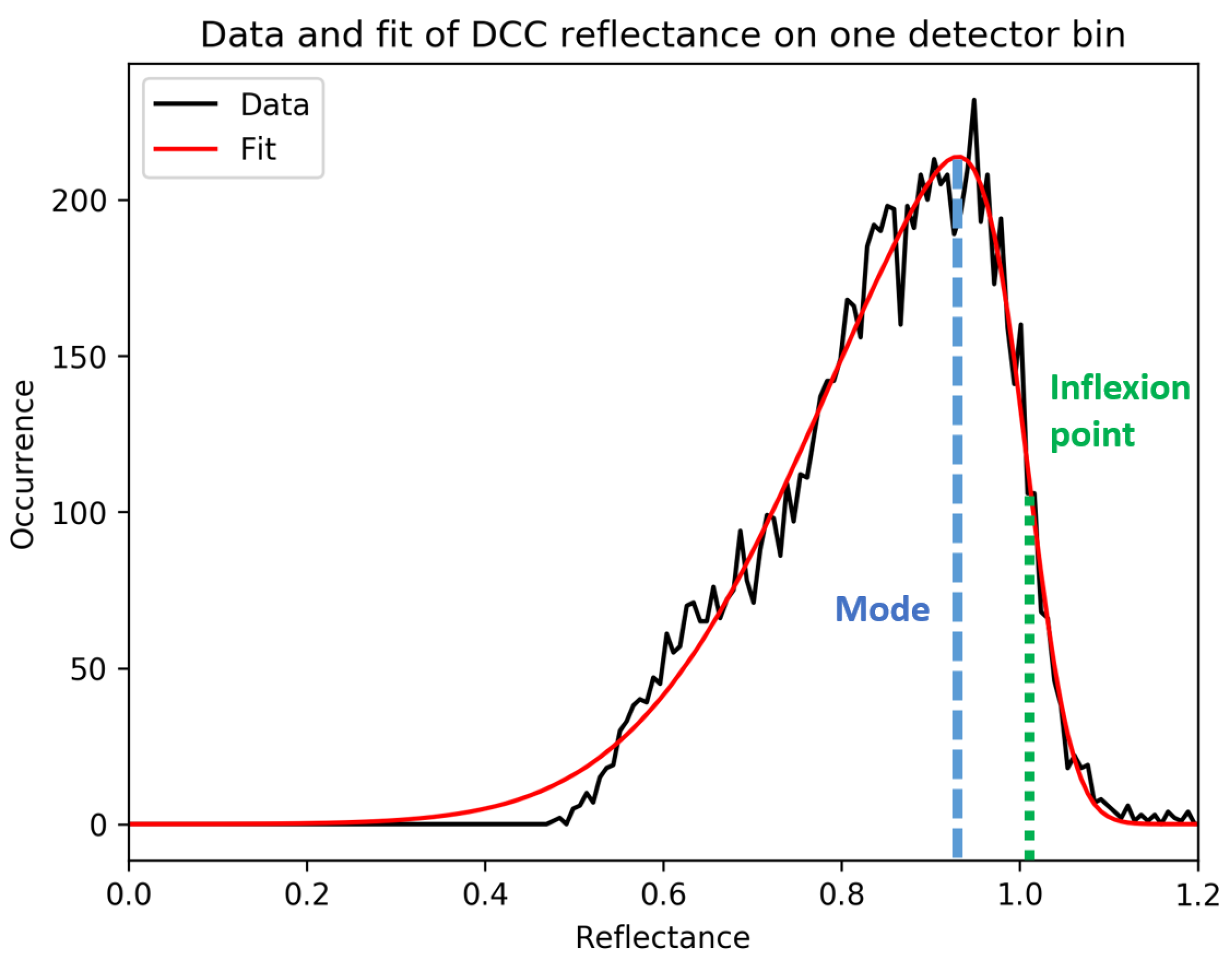
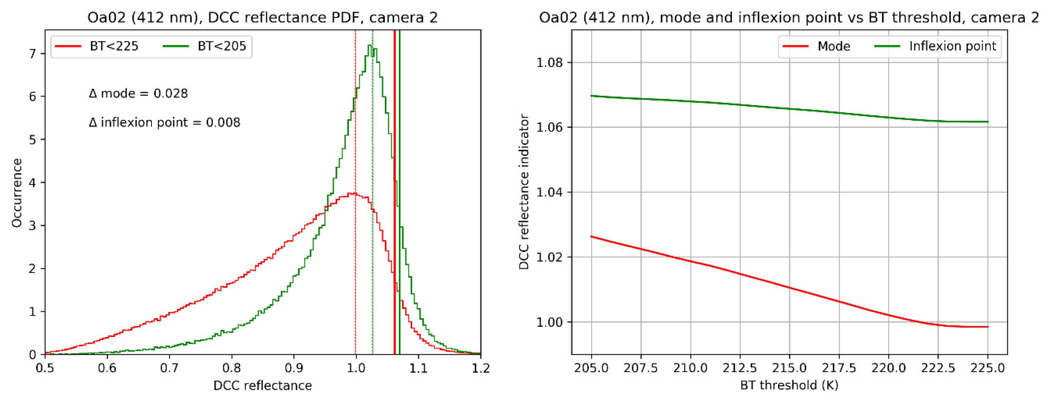
In this study, we propose a rather unusual approach by not considering any other criterion than the selection of low temperature clouds in the Tropics with preliminary threshold at 225 K. Moreover, we make use of the reflectance corresponding to the post-mode inflexion point of the PDF to be used as an indicator for the DCC reflectance distribution instead of the mode. This point should be more representative to conditions of high reflectivity and less sensitive to the sampling of the clouds. Sensitivity analyses are however conducted within the discussion section to validate this approach.

The inflexion point lies in the decreasing slope of the PDF and corresponds to a higher reflectance value than the mode of the distribution. The difference between mode and inflexion point is represented in Figure 13 showing an example distribution, obtained from OLCI for a given detector index, with indication of the positions of the mode and the inflexion point respectively. As it appears, this inflexion point is the strongest gradient in the distribution and is a feature very easy to detect.

To get this inflexion point with best accuracy, each DCC reflectance PDF is modelled as a skewed gaussian distribution [19] with amplitude $\alpha$, center $\mu$, dispersion $\sigma$ and skewness $\gamma$. Such distribution is likely to be the distribution that would be obtained from an ideally large statistics. This has the advantage of removing statistical noise from the original data histograms. Let $\rho$ being the DCC reflectance, the PDF model then writes:

$$f\left(\rho ,\alpha ,\mu ,\sigma ,\gamma \right)=\frac{\alpha }{\sigma \sqrt{2\pi }}{e}^{-\frac{{\left(\rho -\mu \right)}^2}{2{\sigma }^2}}\left(1+\mathrm{erf}\left(\frac{\gamma \left(\rho -\mu \right)}{\sigma \sqrt{2}}\right)\right)$$

(7)

where $\mathrm{erf}$ is the error function [20].

The PDF fit is first performed numerically from a numerical library, then the position of the mode and the inflexion point are retrieved analytically from the retrieved parameters $\left(\alpha ,\mu ,\sigma ,\gamma \right)$. For the sake of legibility, the details of the calculation are provided in the Appendix A.

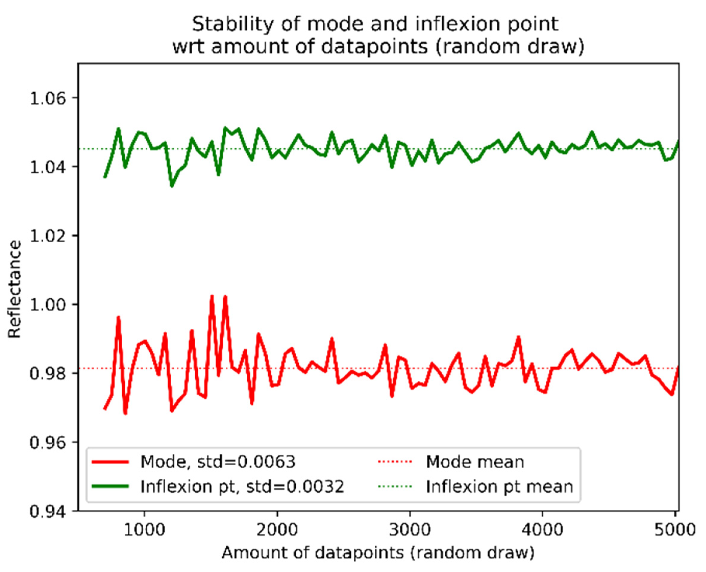
The benefit of using the inflexion point instead of the mode is first validated by performing a random draw on a sample of about 5000 DCC observations. Iteratively, using an increasing number of datapoints from about 500 to 5000, a random sub-sample of this dataset is selected. For each sub-sample a PDF model is fitted on the selected dataset and its mode and inflexion point are retrieved. The variation of their corresponding reflectance values against the number of datapoints is plotted below in Figure 14 in red for the mode and in green for the inflexion point, in the legend are also added the corresponding standard deviations computed from the collection of all individual results, giving an idea of the dispersion around the mean value.

As we can see, the inflexion point provides about half of the dispersion of the mode, which directly translates into a factor two improvement in the precision (i.e., half the uncertainty) on the determination of the DCC reflectance indicator. This will be further validated in the discussion.

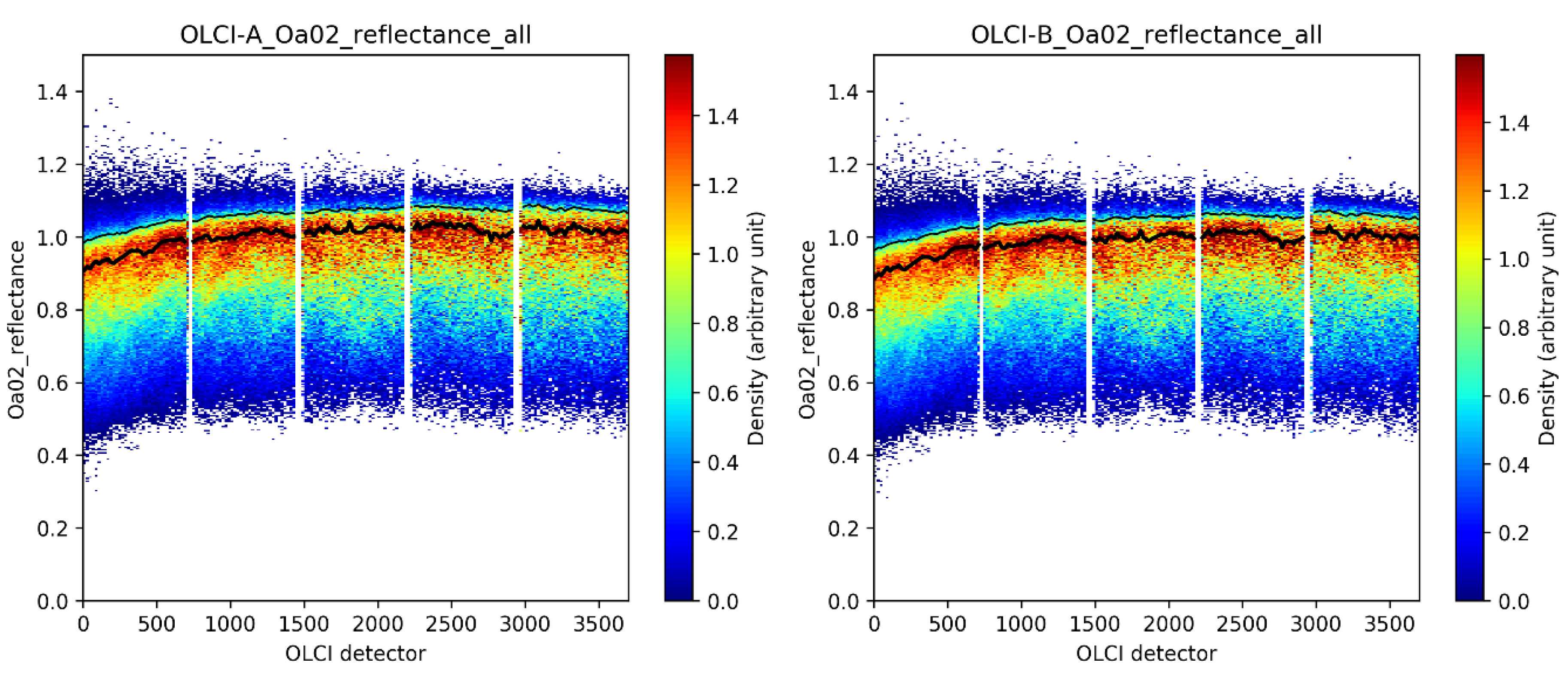
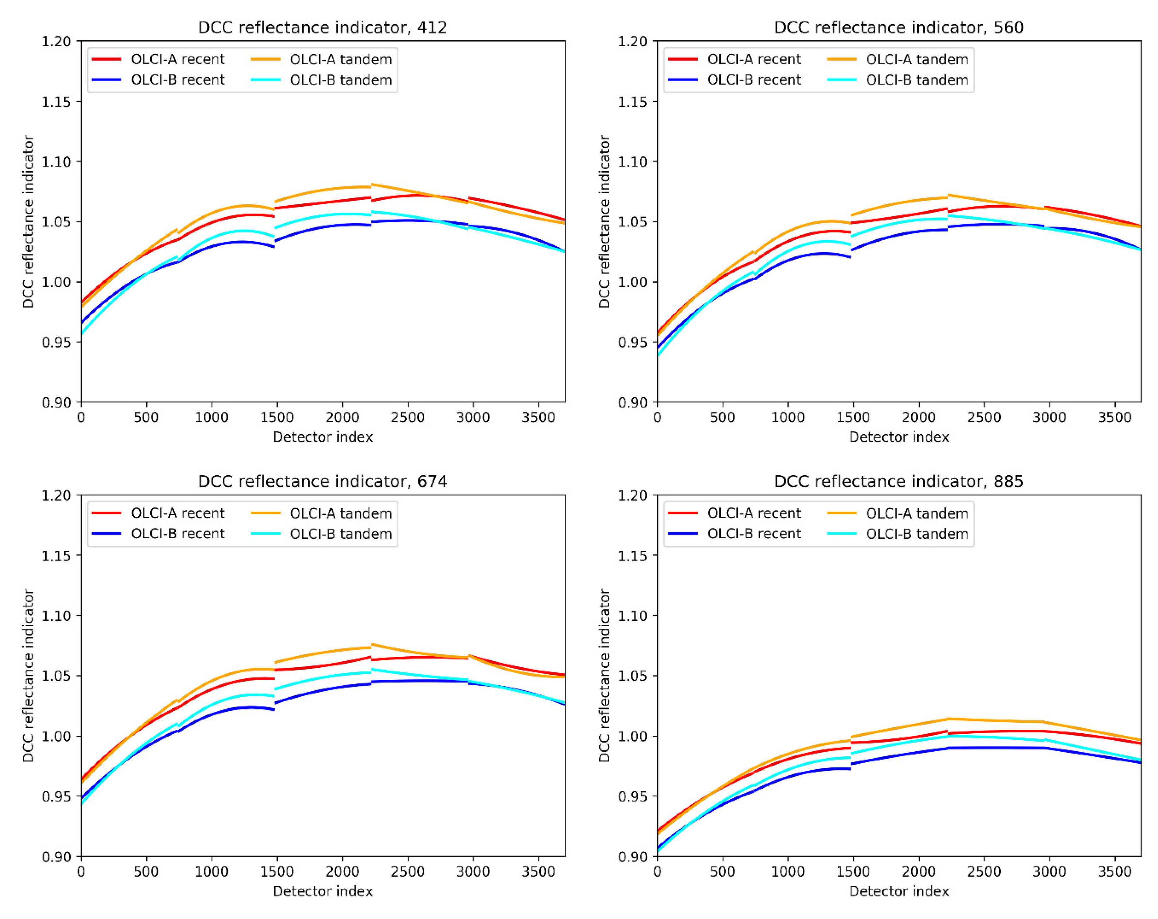
Visual evidence is also shown below when looking at the density of DCC reflectance measurements per OLCI detector index (i.e., the colour scale represents the PDF per detector bin). Figure 15 shows this density for the reference band Oa02 (412 nm) for OLCI-A (left) and OLCI-B (right) obtained from the tandem period along with the corresponding mode (thick line) and inflexion point (thin line corresponding to higher values than the mode). It indeed appears that the inflexion point shows less noise than the mode. At this scale we can only slightly distinguish OLCI-A being slightly brighter than OLCI-B, corroborating the tandem analysis [4]. The other OLCI channels display very similar figures, Supplement Figure S8 provides the visuals corresponding to Figure 15 for the other reference bands Oa06, Oa09 and Oa18.

In the following, we base our analysis directly on the inflexion point values, as reported in the thin lines of Figure 15, for all OLCI bands to the exception of the strong absorption bands. Differences across-track, within and between cameras, are investigated for comparisons with the results of the tandem analysis from [4]. Over the tandem period, the methodology benefits from OLCI-A and OLCI-B sampling exactly the same targets, which helps tuning and validating the method. Out of the tandem, monthly and multi-monthly statistics provide insights on different degrees of precision that can be obtained when the sensors are set on their different orbits and do not acquire the same targets.

4. Results

DCC observations are collected separately over the tandem period and over the more recent period. Results are therefore first presented for the tandem period, then for the other period.

Over any of the two periods, DCC reflectance indicators are computed from all DCC reflectance PDFs obtained per detector index bin, for all bands to the exception of the strong absorption ones, independently for OLCI-A and OLCI-B over three data post-selections:

• Only data without saturated pixels;
• All data, including those saturated pixels, without saturation correction;
• All data, including saturation correction.

4.1. Results from the Tandem Period

Over the tandem period, OLCI-A and OLCI-B collect reflectance from the same DCC targets, only thirty seconds apart. This makes the tandem phase an ideal framework for testing our methodology and especially for assessing the precision of the saturation correction all the more as it does not impact the two sensors with the same magnitude. Cross-calibration between OLCI-A and OLCI-B obtained from the ratio of the individual absolute reflectance indicators can moreover be compared to the “truth” obtained from the tandem analysis in [4]. We recall that such “truth” corresponds to the cross-calibration factors obtained by direct comparisons of homogenised reflectance of OLCI-A and OLCI-B flying in tandem formation with full ACT dependency.

For the sake of brevity, results are first provided in Figure 16 for Oa02 (412, top) and Oa03 (442, bottom) only to highlight the quality of the method in the VIS range, without or with saturated pixels, after correction. The number of saturated pixels per detector bin is mentioned with a black line for OLCI-A and a grey line for OLCI-B.

In the left-hand side, OLCI-A and OLCI-B reflectance indicators clearly exhibit three main characteristics: first, OLCI-A is clearly brighter than OLCI-B; second, the variability ACT exhibits an empirical BRDF highlighting the need to consider OLCI detector indices (i.e., viewing angles) as independently as possible; three, inter-camera differences show up notably with about 2% differences between camera 4 (detectors 2220 to 2959) and camera 5 (detectors 2960 to 3700) consistently with the observations made in [4,5], further providing evidence of inter-camera calibration differences for both OLCI sensors.

In the right-hand side, the relative differences between OLCI-A and OLCI-B indicators (per detector and average per camera) are shown to be equivalent to the results obtained from the tandem analysis which we recall are provided by a statistical analysis of individual ratios of collocated measurements of the two sensors. For Oa03, the correction of the saturated pixels is shown to be very efficient, even for camera 5 where the number of saturated cases is the highest.

Figure 17 now shows the same results for the NIR bands Oa16 (779 nm, top) and Oa17 (865 nm, bottom). The results become less consistent with the tandem results when saturation occurs more often and also as larger uncertainty arise from the interband relationships applied to correct the saturated pixels. We can expect this to be improved for non-saturating sensors and we therefore recommend that sensors are calibrated to avoid saturation over DCCs as much as possible.

Results for all bands are displayed in the Supplement Figures S9 to S14. A synthesis is built up in Figure 18 by displaying the per-camera mean relative differences between OLCI-A and OLCI-B (i.e., as the symbols in the right-hand side of the above figures) along with the associated dispersion obtained from all independent results of a same camera. The left figure shows the absolute values while the right figure shows the difference to the cross-calibration factors of the tandem analysis.

As we can see, most results perfectly match the results from the tandem analysis with differences (sometimes much) lower than 0.5% and very small dispersion. In the NIR, the bands with most uncertainty in the interband relationships used to correct the saturated pixels compare to the tandem analysis with slightly less accuracy, especially at camera 5 where highest saturation rates occur. Results at 1020 nm are the ones with lowest precision and accuracy following the preliminary conclusions on the interband relationships.

However, the very high accuracy (closeness to 0% difference to tandem) and precision (very small dispersion) of these comparisons are mainly because, in tandem formation, both sensors acquire measurements of exactly the same targets. A fortiori, any data selection, applied similarly on both sensors would provide differences only attributable to the difference in calibration and would precisely match the cross-calibration factors obtained from the tandem analysis of [4]. However, with this methodology, it is first interesting to see that applying a statistical analysis of data samples allows to indeed reproduce the result of the tandem analysis. Even more useful, the comparison allows to validate the correction of the saturated pixels, a lack of such correction would indeed cause biases for bands affected by saturation.

Finally, and complementary to the tandem analysis, this methodology allows to trace the ACT variations of an absolute calibration indicator, providing further evidence of calibration residuals between the OLCI cameras, both for OLCI-A and for OLCI-B, as suggested from the analyses at L1 [4] and at L2 [5].

Indeed, the discontinuities between cameras in the ACT profiling of the DCC reflectance indicators are very unlikely to be due to a natural cause. Similarly as in [4], the ratios between the reflectance indicators at each camera interface provide scaling coefficients for each camera to be aligned to its adjacent camera(s). Taking camera 3 as reference allows to propagate these coefficients from camera 3 to camera 2 and then to camera 1 on one side (resp. to camera 4 and to camera 5 on the other side) and obtain flat-fielding factors that compensates the inter-camera calibration differences. Figure 19 shows these factors are derived for OLCI-A (left) and OLCI-B (right).

As we can see, the shape of these factors is similar for both sensors, with somehow more spectral continuity for OLCI-B. As suggested from previous analysis [4] cameras 1 and 5 are the most biased compared to camera 3 taken as reference (although there is no indication to trust more one camera or another), OLCI-B showing the largest bias of about 2% between cameras 4 and 5. Compared to [4] this analysis also provides more detail in the spectral dependency of the factors.

Applying these factors to the ACT profiles of DCC inflexion points in Figure 20 (comparable to e.g., Figure 16) shows how this adjustment provides much more continuity in the profile, exhibiting a much smoother curve now resembling more to what can be expected as an empirical BRDF of the DCCs capturing the average dependency with the viewing angle. We show only the results for the reference bands Oa02, Oa06 and Oa19. It is striking to see the relative differences between OLCI-A and OLCI-B per camera perfectly aligning to a mean bias which depends on the waveband, corroborating the conclusions in [4].

As a full validation of this methodology requires independent measurements from the two sensors, and as the cross-calibration ‘truth’ has been obtained (and shown to be stable in [4]) over the tandem period of acquisition, it would be advantageous to perform an assessment of this method over the tandem period but based on separate acquisitions (e.g., by taking one day over two for each sensor, iteratively). However, only one day of data per week of tandem has been made available for the analysis, only totalising 17 days across the period 25th June 2–15th October. This is rather small to provide a relevant convergence of the method, results of such tests are however provided for information in the Supplement Figure S15, providing only agreement with the tandem analysis better than 1%, sometimes better than 0.5%.

Results obtained out of (even far from) tandem now provide more insights all the more as their investigation is motivated by the long-term monitoring of the cross-calibration factors.

4.2. Results from Out of Tandem Period

We now present results over the recent period (November 2019–May 2020), far from the tandem period. Results are first provided independently for the different months that were collected (one every two months) in order to investigate the variability and uncertainty that can be obtained on a monthly basis.

Interband relationships are inferred from and applied for each month of OLCI products independently to correct the saturated measurements. Most interband ratios obtained over this period are very similar to the ones obtained over the tandem period for each OLCI sensor (see Supplement Figures S16 and S17 for a selection of most interesting cases, and Supplement Figures S18 to S19 for differences to results obtained from the tandem period), to the strong exception of the Oa01 band (400 nm) exhibiting temporal differences principally at camera 3 (individually for OLCI-A and for OLCI-B with opposite signs and amplitude about 0.25%).

These observations highlight the sensitivity of the calibration of the 400 nm band, corroborating the analysis performed in [4], as the solar irradiance gradient is the steepest over this region. As a consequence, the cross-calibration factors obtained over the recent period for Oa01 at camera 3 may differ from the ones obtained over the tandem period.

Indeed, statistics of saturation-corrected DCC observations are shown in Figure 21 through their difference with the cross-calibration factors obtained over the tandem period. Although most channels are packed together per camera, a systematic outlier for Oa01 at camera 3 stands out with an amplitude corresponding to the contributions of both OLCI-A and OLCI-B calibration ‘updates’ as their opposite signs doubles the individual effects of about 0.25% to an outlying 0.5% between Oa01 and (e.g.) Oa02.

Also, the result for Oa21 (1020 nm) is nearly always outlying for all cameras, we suspect that this is rather due to the lack of precision in the reconstruction of the saturated pixels of OLCI-A.

The results for 2019/11 (Figure 21, top-left) provide a remarkably good accuracy with comparisons to tandem analysis lower than 0.5%. Results from the other months of observations appear to be less accurate but also slightly less precise. This may be due to the amount of observations that were found available within the datasets, as shown below in

Table 2. Amount of DCC observations selected for OLCI-A and OLCI-B over the tandem period, each of the four months of analysis, and total of the four months.

	Tandem Period	2019/11	2020/01	2020/03	2020/05	2019/11 to 2020/05
OLCI-A	634 061	1402 281	833 937	929 503	622 865	3788 586
OLCI-B	634 061	1294 497	805 925	966 583	658 691	3725 696

. For instance, the amount of observations for 2019/11 is more than twice the one of 2020/05. The fact that such amounts differ so much between the collected months is rather due to the availability of the data (missing products, temporary unavailability etc.,) than due to the actual variability in the DCC natural geophysical occurrence.

It is to be noted that the figures in Table 2 are representative of the complete OLCI FOV. As this latter is decomposed in 185 bins of 20 detectors, the figures of Table 2 must be interpreted with an average minimum of 3367 datapoints for 2020/05 and an average maximum of 7580 datapoints for 2019/11.

These results show that the method requires a lot of observations to converge as it must cover a large range of the inherent variability of the DCC targets through geographical and temporal sampling. A higher amount of data indeed ensures a better geographical sampling of the natural variability of DCCs. Example differences among two distinct geographical regions are presented in the discussion section, the magnitude of the differences being between about 0.3% for the inflexion point and about 1.5% for the mode.

By comparing to the tandem values, we make the hypothesis that the cross-calibration factors found from the tandem period are still valid far from the tandem, which may however not be the case for Oa01 as revealed from the interband comparisons and for Oa21 because of a lack of accuracy and precision. The observed variability may be due to a combination of the variation in the sensors calibration and different sampling by the two payloads while in operational phase. However, it is striking to see how the result obtained by gathering all observations over the considered period, now in Figure 22, gets much closer to the cross-calibration factors of the tandem analysis with nearly all differences below 0.5% in absolute (still with the exceptions of Oa01 and Oa21), sometimes very close to 0% (cameras 1 and 4).

Although there is no comparison possible with a ‘truth’ obtained over this recent period, this tends to show that radiometric biases between OLCI-A and OLCI-B, with order of magnitude ranging from 2% in the blue to 1% in the NIR, persist even far from the tandem period, even with slight evolution of the calibrations of Oa01 in camera 3, and with less reliability for Oa21.

As obtained from the tandem period, flat-fielding coefficients can also be extracted from the ACT profiles of the DCC inflexion points as shown in Figure 23 (top) along with the differences against the values over the tandem period (bottom). As over the tandem period, camera 3 is brighter than the other cameras, to the exception of few channels. Differences to the tandem values can be as high as 1% but with roughly similar patterns for OLCI-A and OLCI-B.

As for the tandem data, applying the flat-fielding coefficients to the ACT profiles of the DCC inflexion points provides more continuity in the profiles. Partial results are provided in Supplement Figure S20. It is however of better interest to compare these profiles to the ones obtained from the tandem period, which is shown in Figure 24 for the reference channels Oa02 (412 nm), Oa06 (560 nm), Oa09 (674 nm) and Oa18 (885 nm) (Supplement Figure S21 shows the same results for the raw analysis per detector, i.e., without performing flat-fielding, conclusions are similar).

As we can see, the DCC inflexion points show maximum differences of 1% between the two periods, which may be more attributable to variations in the properties of the sampled DCCs rather than to changes in the calibration of OLCI-A and OLCI-B. Indeed, the shape of the profiles for OLCI-A and OLCI-B evolve similarly between the two periods although, after tandem, the two sensors acquire different targets as measuring from different orbital phases. For camera 1 and camera 5 the temporal stability is found better (with or without applying flat-fielding) than for other cameras, which may be attributable to more favourable geometrical conditions, camera 1 being on the edge of the FOV thus looking at clouds from the side, camera 5 rather being in “glint” conditions.

5. Discussion: Sensitivity Analysis and Applicability of the Method to Other Optical Sensors

We discuss here the various assumptions and methodology points that have been employed. First, we have mentioned a preliminary brightness temperature threshold of 225 K for a preselection of DCC pixels. Whereas different thresholds can be used depending on the subject of study (see for instance [21] for a discussion on this matter), the GSICS recommends a threshold of 205 K for selecting convective cores [1]. All results presented above have however sticked to the 225 K threshold, the rationale being the need for wide statistics to handle the sampling into bins of detector index values. We have first tested applying the 205 K criterion without obtaining better results (see Supplement Figure S22 (left panel) corresponding to Figure 22 but restricting to BT < 205 K).

Second, we have made the hypothesis that most variability in the DCC BRDF would be brought by the variation of the sensor viewing angle rather than by the (smaller) variation of the solar zenith angle (SZA). Analyses have all been conducted using binning of the viewing angle ACT but including all possible SZAs. We have tested to down-sample the analysis through the selection of a range of most common SZAs for both OLCI-A and OLCI-B so as to reduce the possible dependency of the clouds BRDF with SZA. Again, we have not found any significant improvement in the results (see Supplement Figure S22, right panel).

More importantly, we have proposed a novel approach by defining the inflexion point of the DCC reflectance PDFs as indicators of the absolute calibration of the OLCI sensors. A preliminary sensitivity analysis has shown that the precision obtained in this indicator is about twice the precision obtained on the mode of the PDFs, i.e., that the dispersion is smaller by a factor 2. Supplement Figure S23 confirms that not only the precision (i.e., the dispersion) is worse but also the accuracy (i.e., the closeness to 0%).

To further highlight the benefit of this approach let us first consider the complete statistics from the recent period of analysis and compute PDFs of the DCC reflectance in the reference band Oa02. Figure 25 below (left-hand side) shows such PDF for a region of the FOV corresponding to the centre of camera 2 when applying either 205 K (green line) or 225 K (red line) BT thresholds. We have added the mode and inflexion points corresponding to each of the two PDFs (resp. dashed and plain vertical lines with colours similar to the corresponding PDF). Clearly, the inflexion point provides more stability with respect to the BT threshold: reported difference between the two PDFs is 0.008 whereas for the modes it is 0.028. Supplement Figures S24 and S25 show similar results for the reference bands as well as for Oa21.

Figure 25 (now right-hand side) also provides the variability of the mode and inflexion points retrieved for each selection of DCC pixels provided by varying the BT threshold between 205 and 225 K. As we see, the variation is smooth and confirms the relative stability of the inflexion point against the mode. Also, when the BT is higher than 222.5 K, the mode and inflexion point reflectance indicators are stable, indicating BT-independence when the BT is higher than 222.5 K. Supplement Figure S26 shows similar results for the same set of bands for (e.g.,) camera 3.

All our analyses are made over the entire globe without restricting to any specific geolocation. Thus, it is of strong interest to reproduce the investigations above but selecting two very different convection areas: Africa (mostly land) and the Tropical Warm Pool (‘Indonesia’, mostly water). Results are provided in Figure 26 similarly as in Figure 25 for the two areas, for the centres of respectively camera 1 (left) and camera 3 (right) which provide most quantitatively different results.

It is striking to see that, for both cameras, the inflexion points (plain vertical lines) are packed with smaller dispersion than the modes (dashed vertical lines). We indicate the differences in modes or inflexion points between the two regions (‘Δ mode’ and ‘Δ inflexion point’) for each of the two BT thresholds. This means that the inflexion point of the distributions is less sensitive to the natural variability of the target. Supplement Figure S27 shows similar results for the same set of bands as above and restricted to (e.g.,) camera 1. Slightly higher sensitivity is found for cameras 2 and 3 (not shown) which can (at least partly) explain the largest discrepancies between monthly results in Figure 21.

In both figures of Figure 26, applying the 205 K threshold provides less dispersion on the modes than applying the 225 K threshold. This becomes advantageous when considering the lack of precision in the reconstruction of the saturated pixels in Oa21: the estimation of the mode relies less on the high values of the reflectance which are more prone to saturation.

Therefore, a final comparison is drawn below in Figure 27 between the results obtained from the inflexion points and BT threshold of 225 K against the results obtained from the mode and BT threshold of 205 K.

Both results are now very similar, to the exception of camera 4 (however still with differences against the tandem lower than 0.5%). Remarkably, and corroborating the previous observations, the alignment of Oa21 is now better (except camera 5) when using the mode and a BT threshold of 205 K. The drawback is however a larger dispersion in the individual results obtained within each camera and leading to a lower precision (see the associated error bars).

As a conclusion, we strongly recommend using the inflexion point technique for OLCI and to test the relevance of this technique to other sensors. The use of the mode, combined to the 205 K BT threshold, however, provides a backup solution for the Oa21 channel when affected by saturation, which may be a recurring matter for the next OLCI sensors.

One other asset of the inflexion point technique is a least sensitivity to the selection of DCC pixels from a BT criterion. All optical sensors do not have access to simultaneous acquisitions of thermal information (e.g., Sentinel-2) and a rough selection of the target could be the sole possibility. For OLCI, it may also be useful to get independent from the selection of DCCs from SLSTR BT measurements at 10.85 µm. An alternative way of getting a proxy for the clouds altitude (and then a sufficient criterion for the method) is given by using the signal from strong absorption bands. From the direct synergy of OLCI and SLSTR Supplement Figure S28 shows the relationships between the TOA reflectance from the two most absorbing bands of OLCI (O₂ band Oa13, 761 nm and H₂O band Oa20, 940 nm) and the BT at 10.85 µm of SLSTR. This shows that the O₂ band provides a rather more linear relationship between TOA reflectance and BT, from which we can say that a threshold of 0.4 on the TOA reflectance provides a selection criterion corresponding to BT < 225 K (resp. 0.6 for BT < 205 K). Similarly, but less precise, a threshold on the H₂O band TOA reflectance of 0.6 can be used (resp. 0.85 for BT < 205 K).

For applicability to other sensors we finally recommend that saturation must be avoided by allowing sufficient dynamics on the detecting devices, notably through designing the sensors to be robust to TOA radiances corresponding to a reflectance up to 1.2. Also, as on-board cloud detection and removal may be considered for data volume reduction of future optical missions, we recommend that DCCs be considered as important targets for radiometric validation and therefore should not be completely removed from the acquisition plan.

6. Conclusions

Throughout this article we have developed and validated a methodology for assessing the cross-calibration of the OLCI sensors (presently OLCI-A and OLCI-B) based on observations of deep convective clouds. The OLCI-A/OLCI-B tandem phase has provided a unique and extremely useful framework for the development and validation of the method, notably regarding the careful handling of saturated pixels impacting more OLCI-A than OLCI-B. Adjustments have been performed from the analysis of interband relationships between bands affected by saturation and reference bands which are not impacted (or are much less impacted) by saturation.

Our method is based on a statistical analysis over monthly to multi-monthly DCC observations datasets with a sampling along the OLCI FOV as this latter provides the largest geometrical variability. No specific selection criterion has been employed for the selection of DCC targets to the exception of a threshold on the 10.85 µm brightness temperatures provided by synergetic measurements from SLSTR. The main finding of this method, leading to better precision and accuracy (at least in our context), is the use of the inflexion point of the DCC PDFs as DCC reflectance indicators for the monitoring of the OLCI-A and OLCI-B radiometry.

This indicator allows to monitor the cross-calibration of the two sensors with accuracy better than 1% on a monthly basis, even better than 0.5% from multi-monthly statistics. More data allowing to more widely sample the natural variability of DCCs that occurs on earth, presently at OLCI observation times. In addition, and complementary to the tandem analysis, this method provides a confirmation as well as a quantification of inter-camera radiometric biases affecting both OLCI-A and OLCI-B.

The results indicate that the cross-calibration of OLCI-A and OLCI-B is temporally stable (within the precision of the method) between the two periods tested in this work (about a year and a half between the two) to the exception of the Oa01 (400 nm) channel and inferred with less precision for the Oa21 (1020 nm) channel. This opens a path toward an operational monitoring and compensation of these calibration differences in the production of the OLCI data, allowing a harmonisation of the ensemble OLCI mission.

We have discussed and validated the assumptions used in this study and made recommendations for applying this method to other optical sensors. Indeed, its basic concepts can be generalised to other OLCI sensors as well as series of optical sensors, currently in the visible and near-infrared spectral domains. It can also be used to improve the precision of the long-term monitoring of the calibration of optical sensors.

Outlooks of this method, among many other opportunities, consider the cross-calibration of the complete Sentinel-3 OLCI mission (from OLCI-A to OLCI-D) when available, the cross-calibration of OLCI and SLSTR visible channels as well as the continuity of calibration between MERIS and OLCI (two very similar instruments yet separated by few years).

For the sake of completeness, a deeper analysis of the regional and temporal variability of the DCCs sampled from OLCI shall provide more insights and possibly even better precision for this method. This is left for future investigations.

References

1. Donlon, C.; Berruti, B.; Buongiorno, A.; Ferreira, M.-H.; Féménias, P.; Frerick, J.; Goryl, P.; Klein, U.; Laur, H.; Mavrocordatos, C.; et al. The global monitoring for environment and security (gmes) sentinel-3 mission. Remote Sens. Environ. 2012, 120, 37–57. [Google Scholar] [CrossRef]
2. Nieke, J.; Borde, F.; Mavrocordatos, C.; Berruti, B.; Delclaud, Y.; Riti, J.-B.; Garnier, T. The Ocean and Land Colour Imager (OLCI) for the Sentinel 3 Gmes Mission: Status and First Test Results. Proc. SPIE 8528, Earth Observing Missions and Sensors: Development, Implementation, and Characterization II, 85280C. Available online: https://www.spiedigitallibrary.org/conference-proceedings-of-spie/8528/85280C/The-Ocean-and-Land-Colour-Imager-OLCI-for-the-Sentinel/10.1117/12.977247.short?SSO=1 (accessed on 30 May 2020).
3. Clerc, S.; Donlon, C.; Borde, F.; Lamquin, N.; Hunt, S.E.; Smith, D.; McMillan, M.; Mittaz, J.; Woolliams, E.; Hammond, M.; et al. Benefits and lessons learned from the sentinel-3 tandem phase. Remote Sens. 2020, 12, 2668. [Google Scholar] [CrossRef]
4. Lamquin, N.; Clerc, S.; Bourg, L.; Donlon, C. OLCI A/B tandem phase analysis, part 1: Level 1 homogenisation and harmonisation. Remote Sens. 2020, 12, 1804. [Google Scholar] [CrossRef]
5. Lamquin, N.; Déru, A.; Clerc, S.; Bourg, L.; Donlon, C. OLCI A/B tandem phase analysis, part 2: Benefits of sensors harmonisation for Level 2 products. Remote Sens. 2020, 12, 2702. [Google Scholar] [CrossRef]
6. Hammond, M.L.; Henson, S.A.; Lamquin, N.; Clerc, S.; Donlon, C. Assessing the effect of Tandem Phase Sentinel 3 OLCI sensor uncertainty on the estimation of potential ocean chlorophyll trends. Remote Sens. 2020, 12, 2522. [Google Scholar] [CrossRef]
7. Lamquin, N.; Woolliams, E.; Bruniquel, V.; Gascon, F.; Gorroño, J.; Govaerts, Y.; Leroy, V.; Lonjou, V.; Alhammoud, B.; Barsi, J.; et al. An inter-comparison exercise of Sentinel-2 radiometric validations assessed by independent expert groups. Remote Sens. Environ. 2019, 233, 111369. [Google Scholar] [CrossRef]
8. Aumann, H.H.; Ruzmaikin, A. Frequency of deep convective clouds in the tropical zone from 10 years of AIRS data. Atmos. Chem. Phys. 2013, 13, 10795–10806. [Google Scholar] [CrossRef] [Green Version]
9. Doelling, D.; Morstad, D.; Bhatt, R.; Scarino, B. Algorithm Theoretical Basis Document (ATBD) for Deep Convective Cloud (DCC) Technique of Calibrating GEO Sensors with Aqua-MODIS for GSICS. Available online: http://gsics.atmos.umd.edu/pub/Development/AtbdCentral/GSICS_ATBD_DCC_NASA_2011_09.pdf (accessed on 30 May 2020).
10. Fougnie, B.; Bach, R. Monitoring of radiometric sensitivity changes of space sensors using deep convective clouds: Operational application to PARASOL. IEEE Trans. Geosci. Remote Sens. 2009, 47, 851–861. [Google Scholar] [CrossRef]
11. Wang, W.; Cao, C. Monitoring the NOAA operational VIIRS RSB and DNB calibration stability using monthly and semi-monthly deep convective clouds time series. Remote Sens. 2016, 8, 32. [Google Scholar] [CrossRef] [Green Version]
12. Lamquin, N.; Bruniquel, V.; Gascon, F. Sentinel-2 L1C radiometric validation using deep convective clouds observations. Eur. J. Rem. Sens. 2017, 51, 11–27. [Google Scholar] [CrossRef]
13. Revel, C.; Lonjou, V.; Marcq, S.; Desjardins, C.; Fougnie, B.; Coppolani-Delle Luche, C.; Guilleminot, N.; Lacamp, A.-S.; Lourme, E.; Miquel, C.; et al. Sentinel-2A and 2B absolute calibration monitoring. Eur. J. Rem. Sens. 2019, 52, 122–137. [Google Scholar] [CrossRef] [Green Version]
14. Coppo, P.; Ricciarelli, B.; Brandani, F.; Delderfield, J.; Ferlet, M.; Mutlow, C.; Munro, G.; Nightingale, T.; Smith, D.; Bianchi, S.; et al. SLSTR: A high accuracy dual scan temperature radiometer for sea and land surface monitoring from space. J. Mod. Opt. 2010, 57, 1815–1830. [Google Scholar] [CrossRef]
15. Bruniquel, J.; Labroue, S.; Féménias, P.; Goryl, P.; Bourg, L.; Rouffi, F.; Smith, D.; Quartly, G.; Bonekamp, H. The Sentinel-3 Mission Performance Center. In Proceedings of the “Sentinel-3 for Science Workshop”, Venice, Italy, 2–5 June 2015. (ESA SP-734, December 2015). [Google Scholar]
16. Thuillier, G.; Hersé, M.; Labs, D.; Foujols, T.; Peetermans, W.; Gillotay, D.; Simon, P.C.; Mandel, H. The solar spectral irradiance from 200 to 2400 nm as measured by the SOLSPEC spectrometer from the ATLAS and EURECA missions. Sol. Phys. 2003, 214, 1–22. [Google Scholar] [CrossRef]
17. McClatchey, R.A.; Fenn, R.W.; Selby, J.E.A.; Volz, F.E.; Garing, J.S. Optical properties of the atmosphere. In Environmental Research Paper, 3rd ed.; Air Force Cambridge Research Laboratory: Bedford, UK, 1972; Volume 411, p. 110. [Google Scholar]
18. Lee, Y.; Ahn, M.-H.; Kang, M. The new potential of deep convective clouds as a calibration target for a geostationary uv/vis hyperspectral spectrometer. Remote Sens. 2020, 12, 446. [Google Scholar] [CrossRef] [Green Version]
19. Azzalini, A. A class of distributions which includes the normal ones. Scand. J. Stat. 1985, 12, 171–178. [Google Scholar]
20. Glaisher, J.W.L. On a class of definite integrals. Lond. Edinb. Dublin Philos. Mag. J. Sci. 1871, 4, 294–302. [Google Scholar] [CrossRef]
21. Yuan, T.; Li, Z. General Macro- and microphysical properties of deep convective clouds as observed by MODIS. J. Clim. 2010, 23, 3457–3473. [Google Scholar] [CrossRef] [Green Version]
Figure 1. Example of a Deep Convective Cloud with collocated OLCI and SLSTR measurements. (Left): OLCI-A reflectance at 412 nm (granule “20180903T081702_20180903T082002”). (Right): SLSTR brightness temperature in S8 channel (10.85 microns).
Remotesensing 12 03105 g001
Figure 2. Close-up on the overshooting region of DCC reflectance at Oa02 (412 nm, left), and Oa03 (442 nm) before (middle) and after masking saturated pixels plus selecting low temperature pixels (right). In the case of OLCI-A (top), saturated pixels (middle image) exhibit very abnormal values in Oa03 (unlike OLCI-B at the bottom).
Remotesensing 12 03105 g002
Figure 3. Average percentage occurrence of saturated pixels from a large sampling of DCC observations per spectral channel and as a function of the detector index within the OLCI FOV. OLCI-A (left) and OLCI-B (right).
Remotesensing 12 03105 g003
Figure 4. Interband statistics and median values (black lines) per OLCI detector for OLCI-A (left) and OLCI-B (right) from the tandem acquisition period. Oa01 (top), Oa03 (bottom).
Remotesensing 12 03105 g004
Figure 5. Interband statistics and median values (black lines) per OLCI detector for OLCI-A (left) and OLCI-B (right) from the tandem acquisition period. Oa04 (top), Oa05 (bottom).
Remotesensing 12 03105 g005
Figure 6. OLCI-A (red) and OLCI-B (blue) spectral characterisation ACT for Oa06 (560 nm) and Oa15 (767 nm).
Remotesensing 12 03105 g006
Figure 7. Interband statistics and median values (black lines) per OLCI detector for OLCI-A (left) and OLCI-B (right) between Oa15 (767 nm) and Oa09 (674 nm) from the tandem acquisition period.
Remotesensing 12 03105 g007
Figure 8. Interband statistics and median values (black lines) per OLCI detector for OLCI-A (left) and OLCI-B (right) between Oa21 (1020 nm) and Oa18 (885 nm) from the tandem acquisition period.
Remotesensing 12 03105 g008
Figure 9. For OLCI-A (left) and OLCI-B (right): Interband relationships between Oa21 (1020 nm) and Oa18 (885 nm) from Figure 8 but as function of the reference reflectance at Oa18 (top) and as function of brightness temperature (bottom) in K. Medians are computed from density histograms, a model applied on the top figures.
Remotesensing 12 03105 g009
Figure 10. Interband relationships for Oa03 (442 nm, top left), Oa04 (490 nm, top right), Oa16 (779 nm, bottom left), and Oa21 (1020 nm, bottom right).
Remotesensing 12 03105 g010
Figure 11. Interband statistics and median values (black lines) per OLCI detector for OLCI-A (left) and OLCI-B (right) from the tandem acquisition period. Oa01 against Oa18.
Remotesensing 12 03105 g011
Figure 12. Statistics of the viewing angle (VZA in degrees, left) and solar zenith angle (SZA in degrees, right) over the tandem phase.
Remotesensing 12 03105 g012
Figure 13. Example probability distribution function of the DCC reflectance (black line) from OLCI DCC observations along with its fit using a skewed-gaussian function (red line). Statistical mode and inflexion point of the distribution are represented.
Remotesensing 12 03105 g013
Figure 14. Mode (red) and inflexion point (green) values obtained over iterative sub-samples of random DCC observation samples of increasing number of datapoints as function of this number. Mean values and standard deviation added in the legend highlighting the better precision of using the inflexion point as a DCC reflectance indicator.
Remotesensing 12 03105 g014
Figure 15. OLCI-A (left) and OLCI-B (right) DCC reflectance (Oa02, 412 nm) distributions per detector index bin (the colour indicates the density of the values) across the FOV. In each detector bin, the fit provides mode (thick black line) and inflexion point (thin black line) of the distribution.
Remotesensing 12 03105 g015
Figure 16. (Left): OLCI-A (orange to deep red) and OLCI-B (light to deep green) DCC reflectance indicators for bands Oa02 (412 nm) and Oa03 (442 nm) for the three data selections. (Right): corresponding relative differences between OLCI-A and OLCI-B for the three data selections (full dependency ACT and mean) with comparisons to tandem analysis results from [4]. In both left and right panels, black (OLCI-A) and grey (OLCI-B) lines indicate the amount of macropixels which are partially saturated.
Remotesensing 12 03105 g016
Figure 17. (Left): OLCI-A (orange to deep red) and OLCI-B (light to deep green) DCC reflectance indicators for bands Oa16 (779 nm) and Oa17 (865 nm) for the three data selections. (Right): corresponding relative differences between OLCI-A and OLCI-B for the three data selections (full dependency ACT and mean) with comparisons to tandem analysis results from [4]. In both left and right panels, black (OLCI-A) and grey (OLCI-B) lines indicate the amount of macropixels which are partially saturated.
Remotesensing 12 03105 g017
Figure 18. (Left): per-camera mean and associated standard deviation of the DCC methodology for all OLCI bands. (Right): same but relative to the tandem analysis cross-calibration factors. DCC results obtained over the tandem period.
Remotesensing 12 03105 g018
Figure 19. Flat-fielding factors obtained for OLCI-A (left) and OLCI-B (right) over the tandem period.
Remotesensing 12 03105 g019
Figure 20. Same as Figure 16 and Figure 17 but for reference bands Oa02 (412 nm), Oa06 (560 nm) and Oa19 (900 nm), after empirical alignment of the cameras.
Remotesensing 12 03105 g020
Figure 21. Per-camera mean and associated standard deviation of the cross-calibration factors obtained from the DCC methodology for all OLCI bands, differences to the tandem analysis cross-calibration factors. Top-left: period 2019/11, top-right: period 2020/01, bottom-left: period 2020/03, bottom-right: period 2020/05.
Remotesensing 12 03105 g021
Figure 22. Left: per-camera mean and associated standard deviation of the DCC methodology for all OLCI bands. Right: same but comparisons to the tandem analysis cross-calibration factors. Results obtained over the recent period (all months combined).
Remotesensing 12 03105 g022
Figure 23. Flat-fielding factors (top) obtained for OLCI-A (left) and OLCI-B (right) over the recent period (all months combined) along with their difference to the same factors obtained over the tandem period (bottom).
Remotesensing 12 03105 g023
Figure 24. OLCI-A (red over the recent period, orange over the tandem period) and OLCI-B (blue over the recent period, cyan over the tandem period) DCC reflectance indicators for bands Oa02 (412 nm), Oa06 (560 nm), Oa09 (674 nm) and Oa18 (885 nm) after flat-fielding adjustment.
Remotesensing 12 03105 g024
Figure 25. (Left): Oa02 DCC reflectance PDFs for one region of the FOV (centre of camera 2) for the two BT thresholds (205 and 225 K) with corresponding mode and inflexion points reported in (resp.) dashed and plain lines. (Right): variation of the mode and inflexion points retrieved in similar conditions but varying the BT threshold between 205 and 225 K.
Remotesensing 12 03105 g025
Figure 26. Same as Figure 25 but separating the analysis into Africa and Indonesia convective regions. (left): camera 1; (right): camera 3.
Remotesensing 12 03105 g026
Figure 27. Comparison between the results from Figure 22 (i.e., obtained from inflexion point statistics and a BT threshold of 225 K) and the results obtained from using mode statistics and a BT threshold of 205 K.
Remotesensing 12 03105 g027