Article

Using Machine Learning for Estimating Rice Chlorophyll Content from In Situ Hyperspectral Data

1
School of Resources and Environment, University of Electronic Science and Technology of China, Chengdu 611731, China
2
Center for Information and Geoscience, University of Electronic Science and Technology of China, Chengdu 611731, China
3
Department of Geography, Western University, London, ON N6A 5C2, Canada
4
Applied Geosolutions, 15 Newmarket Road, Durham, NH 03824, USA
5
Ottawa Research and Development Centre, Agriculture and Agri-Food Canada, 960 Carling Avenue, Ottawa, ON K1A 0C6, Canada
6
Crop Research Institute, Sichuan Academy of Agricultural Sciences, Chengdu 610066, China
*
Author to whom correspondence should be addressed.
Remote Sens. 2020, 12(18), 3104; https://doi.org/10.3390/rs12183104
Submission received: 6 August 2020 / Revised: 19 September 2020 / Accepted: 20 September 2020 / Published: 22 September 2020
(This article belongs to the Special Issue Remote Sensing for Precision Agriculture)

Abstract

:
Chlorophyll is an essential pigment for photosynthesis in crops, and leaf chlorophyll content can be used as an indicator for crop growth status and help guide nitrogen fertilizer applications. Estimating crop chlorophyll content plays an important role in precision agriculture. In this study, a variable, rate of change in reflectance between wavelengths ‘a’ and ‘b’ (RCRWa-b), derived from in situ hyperspectral remote sensing data combined with four advanced machine learning techniques, Gaussian process regression (GPR), random forest regression (RFR), support vector regression (SVR), and gradient boosting regression tree (GBRT), were used to estimate the chlorophyll content (measured by a portable soil–plant analysis development meter) of rice. The performances of the four machine learning models were assessed and compared using root mean square error (RMSE), mean absolute error (MAE), and coefficient of determination (R2). The results revealed that four features of RCRWa-b, RCRW551.0–565.6, RCRW739.5–743.5, RCRW684.4–687.1 and RCRW667.9–672.0, were effective in estimating the chlorophyll content of rice, and the RFR model generated the highest prediction accuracy (training set: RMSE = 1.54, MAE =1.23 and R2 = 0.95; validation set: RMSE = 2.64, MAE = 1.99 and R2 = 0.80). The GPR model was found to have the strongest generalization (training set: RMSE = 2.83, MAE = 2.16 and R2 = 0.77; validation set: RMSE = 2.97, MAE = 2.30 and R2 = 0.76). We conclude that RCRWa-b is a useful variable to estimate chlorophyll content of rice, and RFR and GPR are powerful machine learning algorithms for estimating the chlorophyll content of rice.

Graphical Abstract

1. Introduction

In recent years, precision agriculture has been gaining momentum [1]. Rice is one of the three major food crops in the world and covers the largest planting area in China [2]. Therefore, monitoring the phenotypic information of rice plays an important role in precision agriculture. In the photosynthesis process, chlorophyll is an essential pigment whose content is related to the phenology and health status of crops [3]. Besides, the chlorophyll content is close to the nitrogen nutritional status of crops, since most part of nitrogen was contained in chlorophyll [4]. As a result, crop chlorophyll content can indirectly predict soil nitrogen conditions and guide the application strategy of nitrogen fertilizer, which can increase the overall crop profitability.
Previous studies have revealed that remote sensing is a reliable and effective technology for obtaining crop biophysical and biochemical information [5,6,7]. In particular, hyperspectral remote sensing has narrow and continuous spectral bands, providing almost continuous spectra, which is more sensitive to specific vegetation properties such as nitrogen status, canopy biomass, and chlorophyll content [5,8]. Many studies have developed a large number of spectral indices to estimate the chlorophyll content of crops based on hyperspectral remote sensing reflectance [9,10,11]. Although most of these spectral indices perform well in estimating crop chlorophyll content, it is difficult to interpret their physical meanings as most of them are in normalized radio or normalized difference form. In addition, the first derivative of a spectrum, having physical interpretability that can indicate the rate of change in reflectance, was widely used to evaluate crop chlorophyll content [12,13]. However, the first derivative of a spectrum can only reflect the rate of change in reflectance near a specific wavelength on the micro level. Some other information, such as the rate of change of reflectance within a wavelength range, is ignored, which may provide more sensitive information for the chlorophyll content estimation. As a result, the rate of change in reflectance between wavelengths ‘a’ and ‘b’ (RCRWa-b), proposed in this study, is the promotion of first derivative of spectrum, which can not only reflect the rate of change in reflectance at a certain wavelength, but also the rate of change in reflectance between any two wavelengths.
The processing techniques used for retrieving vegetation characteristics can be divided into two broad groups: physically-based algorithms and empirically-based algorithms [14,15]. Compared with physically-based algorithms, such as PROSAIL [16] and N-PROSAIL [17], empirically-based algorithms have low complexity, high computational efficiency, fewer required variables, and provide reliable results [15,18]. Empirically-based algorithms, especially machine learning algorithms, including random forest (RF) [19], support vector regression (SVR) [20,21], neural networks (NNs) [22,23], and the Gaussian process (GP) [24,25], have been widely used to evaluate chlorophyll content of vegetation. However, few studies have investigated and compared the performance of different machine learning algorithms in estimating the chlorophyll content of vegetation. In addition, the optimization process of some key hyperparameters that can greatly affect the performance of machine learning algorithms, was not deep studied or ignored in previous study.
Therefore, this study has two major objects: (1) investigating the potential of the rate of change in reflectance between wavebands in estimating the chlorophyll content of rice; and (2) comparing the performance of four advanced machine learning technology, GP, RF, SVR and gradient boosting regression tree (GBRT), in estimating the chlorophyll content of rice.

2. Materials

2.1. Experimental Site and Experimental Design

Field experiments were conducted at the Modern Agricultural Science and Technology Innovation Demonstration Park of Sichuan Academy of Agricultural Sciences, Chengdu, Sichuan, China (Figure 1a). Multi-temporal field campaigns were conducted between 12 July and 17 September in 2019 (Table 1). In this study, two rice fields (marked as 1, 2 in Figure 1b and labeled as Field1 and Field2, respectively) were selected. There are hundreds of plots in Field1, and each plot was planted with a different rice cultivar. Field2 is a replication of Field1, and the two fields had the same planting density (26.67 cm × 20.00 cm) and received the same irrigation, and field managements. The spatial distribution of sample plots is illustrated in Figure 1b.

2.2. Data Acquisition

In this study, spectral measurements of rice plants were collected using a PSR 3500 spectroradiometer (Spectral Evolution Inc., Lawrence, MA, USA) at 0.2 m above the top of the canopy. Before each measurement, a white reference panel with a reflectance of 99% was used for calibration. The spectroradiometer used covers the wavelength of 350–2500 nm, and the spectral resolutions are 3 nm at 700 nm, 8 nm at 1500 nm, and 6 nm at 2100 nm. Besides, after the spectroradiometer completed one set of measurements, the instrument resamples the spectra by 1.3 nm at 350–1000 nm, 3.5 nm at 1000–1800 nm and 2.5 nm at 1800–2500 nm. Within each sample plot, three sampling points were random selected. At each sampling point, ten reflectance spectra were measured resulting in a total of 30 spectra; the average of the thirty reflectance spectra was then used to represent the reflectance spectra of the sample plot. To minimize atmospheric perturbations and BRDF effects, all spectral measurements were measured on clear sunny days between 11:30 a.m. and 2:00 p.m. [5]. Previous studies have demonstrated the capability of soil–plant analysis development (SPAD) value for plant chlorophyll content estimation [5,26,27,28]. In this study, a non-destructive and portable SPAD meter (SPAD-502 Plus, Konica Minolta Sensing Inc., Osaka, Japan) was used to collect measurements of light absorptions of the leaf at two wavelengths (650nm and 940 nm) [1]. At each sample plot, three leaves of the top layer were randomly selected, and two measurements were taken at the middle and top of each leaf. As a result, the average of the six measured SPAD values was used as the final measurement representing that sample plot.

3. Methodology

3.1. Theoretical Background

3.1.1. Gaussian Process Regression

Gaussian process regression (GPR) is a powerful machine learning algorithm and has been widely used in remote sensing community, including estimating aboveground forest biomass [29] and soil salinity [30]. GPR is suitable for solving problems with a small sample size; when the sample size is large or has high dimensional features it becomes inefficient. In the GPR model, a relationship was established between the input variables x i = [ x ( 1 ) , x ( 2 ) , , x ( B ) ] and output variable y R using the following equation [31]:
y = f ( x ) = i = 1 n α i K ( x i , x )
where x i is the explanatory variable used at the training stage; n is the number of samples; α i is the weight coefficient, and K is the radial basis kernel function (RBF), whose equation is as follows:
K ( x i , x j ) = β exp ( b = 1 B ( x i ( b ) x j ( b ) ) 2 / ( 2 σ b 2 ) )
where β is a scaling factor, B is the number of input explanatory variables (B was set at 4 in this study, see Section 4.1), and σ b is a dedicated parameter controlling the spread of the relations for each particular input variable [31]. Three model parameters ( β , α i , σ b ) can be automatically optimized by maximizing the marginal likelihood in the training set [31,32].

3.1.2. Random Forest Regression

Random forest (RF) is an ensemble learning method based on multiple decision trees, which combines Breiman’s idea of "bagging" and random selection of features [33,34]. The following steps are needed to build a RF model. Firstly, based on the training dataset, a homogeneous subset is generated by bootstrap aggregation algorithm. Then, by selecting random samples and variables from the calibration dataset, each sub decision tree is grown to its maximum depth, and this process can be executed in parallel. Finally, all of the sub decision trees are put together to generate a random forest model [30,33]. When building a random forest model, it is necessary to determine two parameters, the number of decision trees in the bagging framework and the number of variables in the decision tree framework [30]. RF algorithm has a strong anti-over-fitting capability without losing information, and can always lead to the convergence of generalization error, which has been used in many previous studies on chlorophyll [33]. Random forest regression (RFR) is the regression version of RF.

3.1.3. Support Vector Regression

Support vector regression (SVR) is the regression version of the support vector machine, which has been developed on the basis of statistical learning theory [35]. It fits an optimized hyper-plane to a set of input features to establish a linear dependency between n-dimensional input variables and a one-dimensional target variable. Kernel function maps training samples to high-dimensional features that are nonlinearly related to the original feature space and enables the new data distribution to fit into a linear model [36]. In SVR, there are four kinds of kernels: linear, polynomial, Gaussian, and sigmoid [37]. In the field of remote sensing, the Gaussian kernel has been widely used [33,36] and was selected in this study. In SVR, the kernel parameter (gamma) and regulation parameter (C) can affect the performance of the model [31]. Therefore, the two parameters C and gamma should be correctly determined.

3.1.4. Gradient Boosting Regression Tree

The gradient boosting algorithm, a machine learning technique, is an optimization algorithm based on the error function and can be used to solve classification and regression problems [38]. It can generate a strong prediction model by integrating weak prediction models, such as the decision tree [38]. The gradient boosting regression tree (GBRT) is an iterative decision tree algorithm composed of multiple decision trees, which makes GBRT difficult for parallel computing. The core idea of the GBRT is that each calculation is done by a basic model, and the subsequent calculation is undertaken to reduce the residual of previous model and to create a new basic model in the direction of gradient with reduced residuals [38,39]. Therefore, a strong prediction model can be obtained by adjusting the weight of the weak prediction model. In the meanwhile, the loss function can be minimized [38]. Typical parameters of GBRT include learning rate (a contribution extent of each decision tree), n-estimators (the number of sub-decision tree), and max depth (the maximum depth of a sub-decision tree) et al.

3.1.5. Cross Validation and Parameter Optimization

Cross validation (CV) is a statistical analysis method to test the performance of the regression model. The basic idea is to group the original sample data, and take one set of data samples as validation set and the other as training set. K-fold cross validation is a common cross validation method. In this study, K was set as 8.
Grid search (GS) is a parameter adjustment algorithm. For each combination in the parameter combination list, the GS instantiates the given model, performs K cross validation, and takes the parameter combination with the highest average score as the best choice. In the regression problem, mean square error (MSE) is normally used to evaluate the model performance and was selected in this study. In general, the smaller the MSE, the better the performance of the model.
In this study, GS combined with CV, labeled GS-CV, was used to select optimal parameters.

3.1.6. Performance Assessment

The performance of four machine leaning algorithms, GPR, RFR, SVR and GBRT, were assessed and compared using statistical metrics including root mean square error (RMSE; Equation (3)), mean absolute error (MAE; Equation (4)) and the coefficient of determination (R2; Equation (5)).
RMSE is considered a standard metric for measuring errors of regression models. It is significantly influenced by large values and outliers of the input data [31,40]. Therefore, RMSE and MAE were combined to evaluate the variation of model errors. The higher R2, lower RMSE, and lower MAE indicate a better model. Furthermore, the smaller the difference between RMSE and MAE, the smaller the variance between the errors [31].
RMSE = i = 1 n ( y i ^ - y i ) 2 n
MAE = 1 n i = 1 n | y i - y i |
R 2 = 1 - i = 1 n ( y i - y i ) 2 i = 1 n ( y i - y ¯ ) 2
where y i and y i are the computed and measured SPAD values of the i - t h sample respectively; y ¯ is the mean values of the measured SPAD values; and n is the total number of samples used.

3.2. The Rate of Change in Reflectance between Wavelengths ‘a’ and ‘b’

To estimate rice chlorophyll content, rate of change in reflectance between wavelengths ‘a’ and ‘b’ (labeled as RCRWa-b) was defined as the slope ( w ) of the straight line:
y = w x + c
where the equation of w is:
w = i = 1 m y i ( x i x ¯ ) i = 1 m x i 2 1 m ( i = 1 m x i 2 ) 2
where x i is the i t h wavelength between wavelength ‘a’ and ‘b’, y i is the reflectance corresponding to x i , and m is the number of wavelength between wavelength ‘a’ and ‘b’.
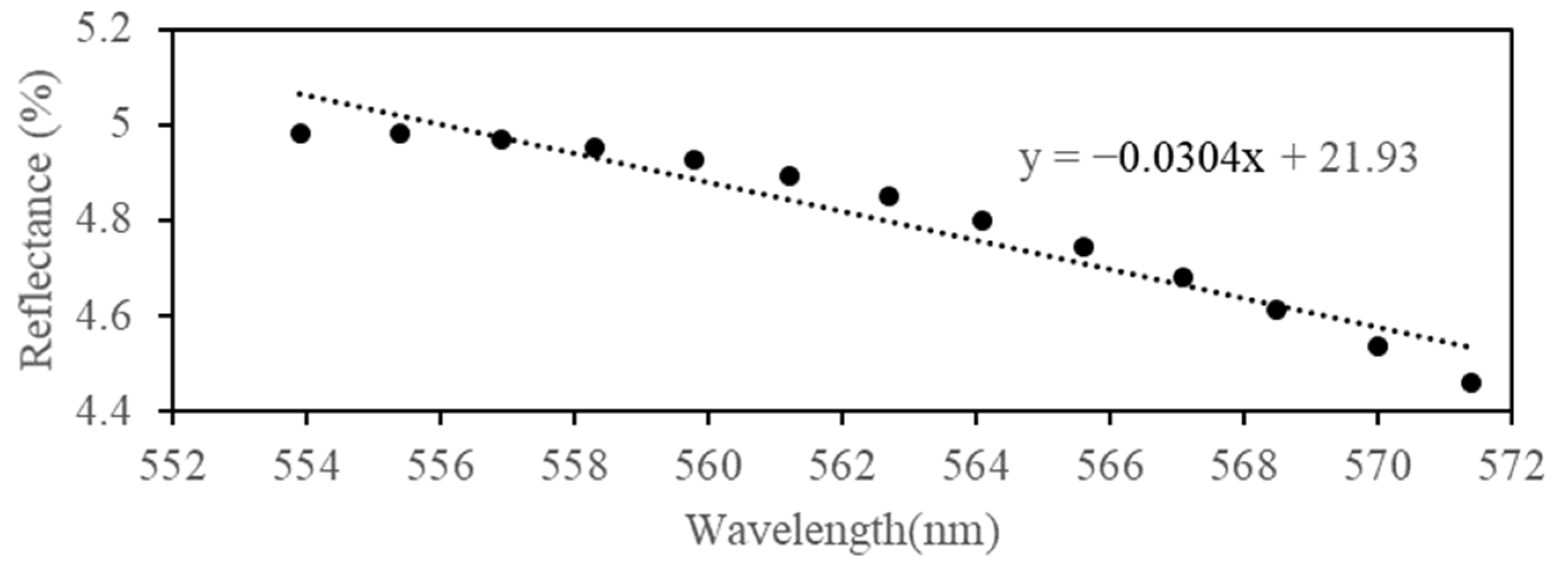
In other words, RCRWa-b is the slope of one straight line that obtained by linear fitting the wavelengths (from ‘a’ to ‘b’) and reflectance corresponding to wavelengths (from ‘a’ to ‘b’). For example, Figure 2 shows the rate of change in reflectance between wavelengths 553.9 nm and 571.4 nm (labeled as RCRW553.9–571.4), which is −0.0304.

3.3. Analytical Framework

Figure 3 gives the workflow of the proposed methodology used in this study for estimating the chlorophyll content of rice plants. Firstly, features of RCRWa-b were obtained by preprocessing the in situ hyperspectral data. Secondly, the coefficient between RCRWa-b and SPAD value was calculated. Thirdly, four features of RCRWa-b were selected according to the correlation coefficient between RCRWa-b and SPAD value. Then, the rice SPAD estimation database was divided into training and validation sets. Next, four machine learning models were established based on GS-CV and the training set. Finally, the performances of the four models were assessed and compared. Section 4.1 and Section 4.2 show the details.

4. Results

4.1. Features Selection

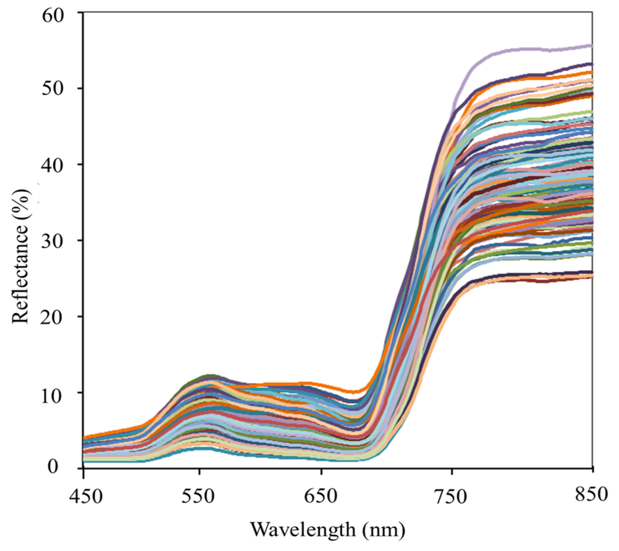
Previous studies have shown that there is a strong correlation between the first derivative reflectance of plants at 500 nm to 750 nm and the chlorophyll content of plants [12,13]. In addition, some vegetation indices (see in Table 2, [41,42]), derived from the green, red, red-edge, and near infrared (NIR) bands were used to estimate the chlorophyll content of vegetation. Moreover, spectral wavebands in the green band (500–580 nm), red band (630–690 nm), and red age band (700–750 nm) region are considered to be the useful range for estimating chlorophyll content [4,43,44,45,46]. Therefore, the reflectance between 500 nm and 800 nm is the preferred wavelength range to estimate the chlorophyll content of plants. Figure 4 shows all of the spectra measured between 450 nm and 850 nm (500–800 nm are useful range).
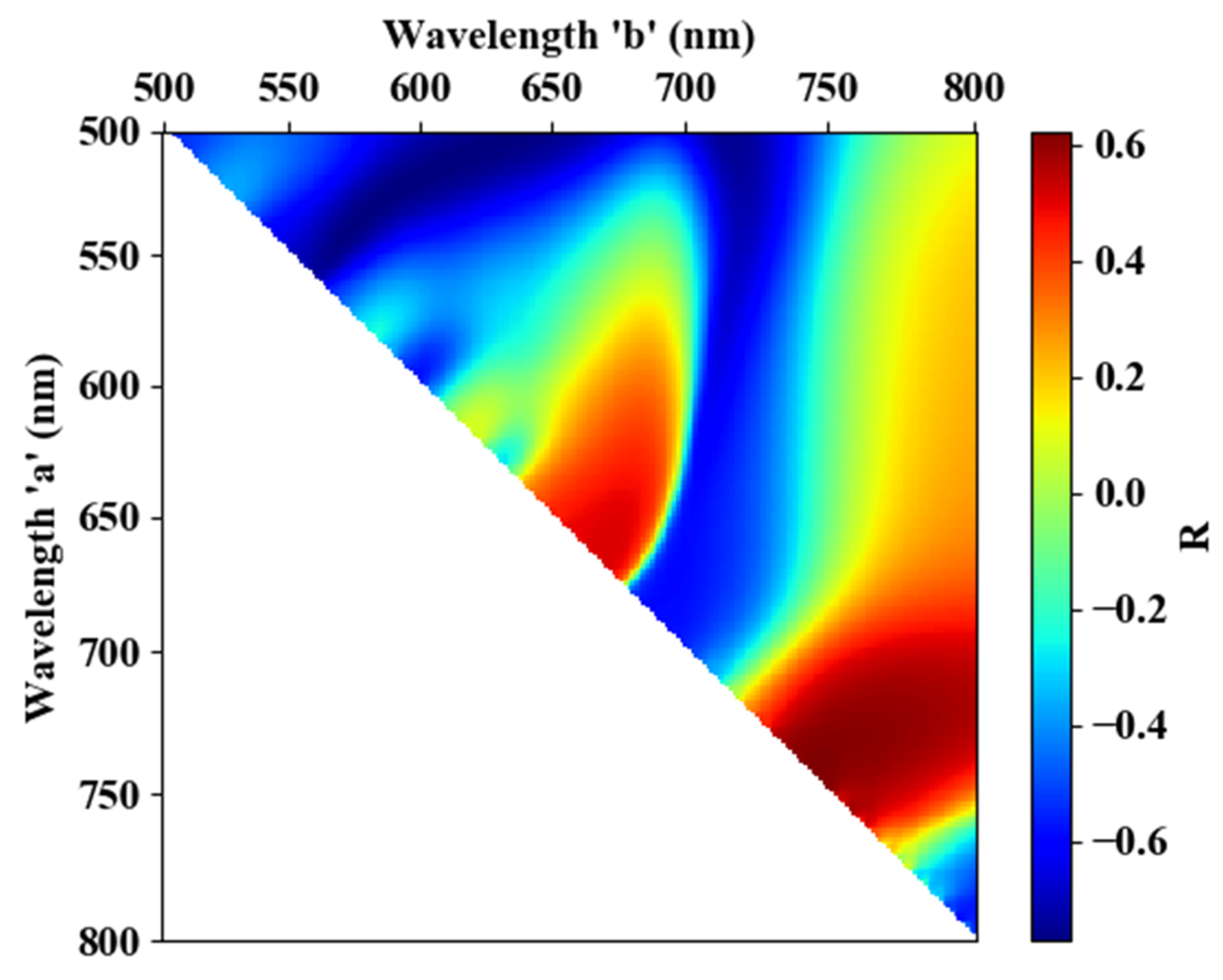
In this study, the correlation coefficient (R) between RCRWa-b and SPAD value was calculated, and the correlogram is shown in Figure 5. In Figure 5, the ranges of ‘a’ and ‘b’ are both from 500nm to 800 nm with ‘b’ > ’a’. According to Figure 5, there is a strong correlation between RCRWa-b and SPAD value when ‘a’ and ‘b’ are: (1) both in green bands; (2) both in red bands; (3) both in red edge bands; or (4) both in NIR bands.
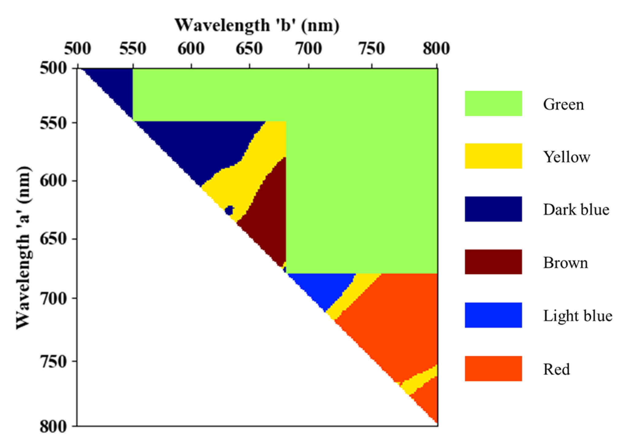
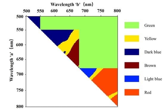
However, there are some features of RCRWa-b that do not have obvious physical significance. For example, when the ‘a’ and ‘b’ of RCRWa-b are 520 nm and 640 nm respectively (See in Figure 6a), there is a peak reflectance between 520 nm and 640 nm where the reflectance rises firstly and then falls. In this case, the RCRWa-b cannot reflect the change rate of reflectance between 520 nm and 640 nm. When ‘a’ and ‘b’ of RCRWa-b are 600 and 700 nm respectively (see in Figure 6b), RCRWa-b also does not have obvious physical significance, because there is a trough between 600 nm and 700 nm. Therefore, the features of RCRWa-b were not considered when both ‘a’ and ‘b’ fell under the following conditions (there is a crests or troughs in Condition 1 and Condition 2): Condition 1: a < 550 nm and b > 550 nm; Condition 2: 550 nm < a < 680 nm and b > 680 nm. The range of wavelength ‘a’ and ‘b’ corresponding to these two conditions are shown in Figure 7 in green.
In addition, although some RCRWa-b have obvious physical significance, they were removed because the correlation between SPAD and they are poor (abs(R) < 0.2), and the range of wavelength ‘a’ and ‘b’ of these RCRWa-b were shown in Figure 7 in yellow.
To choose effective features and reduce data redundancy, we calculated the correlation coefficient between the features of adjacent wavelengths. Figure 8 depicts that there is a strong correlation between two RCRWa-b with adjacent wavelengths (in Figure 8a, 536.3 nm is close to 540.7 nm and 543.7 nm is close to 549.5 nm; in Figure 8b, 658.2 nm is close to 662.3 nm, and 665.1 nm is close to 670.6 nm). Therefore, it was necessary to remove redundant features and select only a few features.
In this study, some RCRWa-b that have no obvious physical significance were removed. Besides, since there is multicollinearity between two RCRWa-b with adjacent ‘a’ or ‘b’, we select one feature with the strongest correlation with SPAD in each of the following four conditions (from Condition (1) to Condition (4), the correlation between SPAD and RCRWa-b alternated between positive correlation and negative correlation):
  • Condition (1): the range of wavelength ‘a’ and ‘b’ of RCRWa-b is shown in Figure 7 in dark blue;
  • Condition (2): the range of wavelength ‘a’ and ‘b’ of RCRWa-b is shown in Figure 7 in brown;
  • Condition (3): the range of wavelength ‘a’ and ‘b’ of RCRWa-b is shown in Figure 7 in light blue;
  • Condition (4): the range of wavelength ‘a’ and ‘b’ of RCRWa-b is shown in Figure 7 in red;
As a result, four features were selected, which are RCRW551–565.6, RCRW739.5–743.5, RCRW684.4–687.1, and RCRW667.9–672, and the four selected RCRWa-b were labeled as Four-RCRWa-b. The scatter plots between SPAD readings and the four selected RCRWa-b are shown in Figure 9.

4.2. Model Configuration and Training

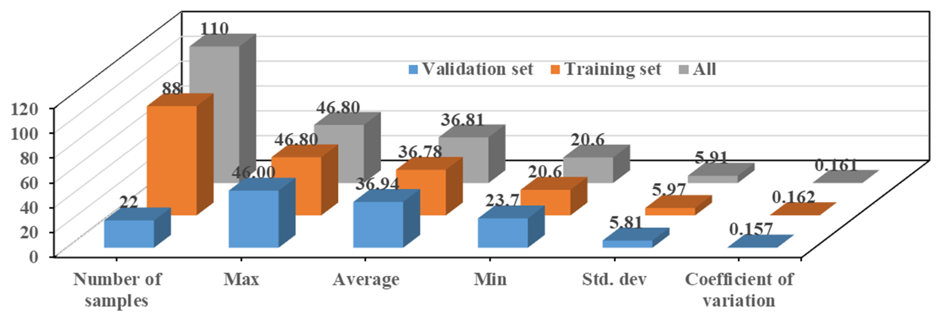
In this study, the random stratified sampling method was used to divide the dataset into a training set (80%) and a validation set (20%). In addition, a fixed seed of random numbers was used to make the training dataset and validation dataset of all generated models fixed. The statistical characteristics of the dataset are shown in Figure 10. As can be seen in Figure 10, some statistical characteristics such as, mean (36.94 and 36.78), max (46.00 and 46.80), min (23.7 and 20.6), standard deviation (5.81 and 5.97), and coefficient of variation (0.157 and 0.162), of the validation set and training set are close. Moreover, the data distribution of the training and validation set, a significant factor influencing the model performance, is consistent with the total data set, since the statistical characteristics of them is close.
Using the training set and GS-CV, configurations of those four machine learning models were optimized.
For the Gaussian process regression model, the hyper parameters: β , α i , and σ b (see in Section 3.1.1) were automatically optimized during the training process and the generated Gaussian Process Regression Model was referred to GPR-M.
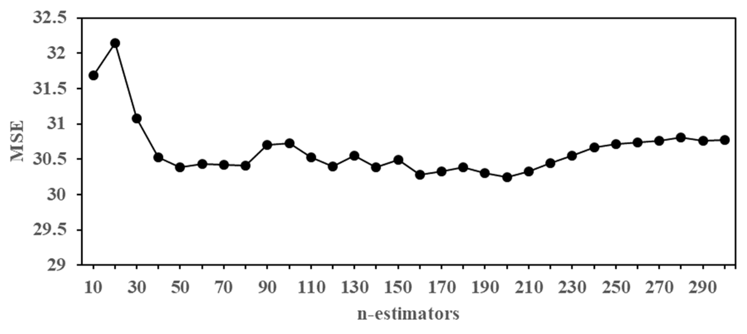
For the random forest regression model, the number of features was set to four, which is equal to the number of input features when establishing the sub-decision trees. Another parameter, the number of sub-decision trees (n-estimators), was determined based on GS-CV. In addition, some parameters such as the max depth of sub-decision trees, the minimum number of samples for leaf nodes and other parameters are the default value from the “sklearn.ensemble.RandomForestRegressor” of the Python toolkit: scikit-learn 0.22. The MSE of models with different n-estimators is shown in Figure 11. According to Figure 11, when n-estimator is 200, the generated RFR model referred to as RFR-M achieves the smallest MSE. Besides, the importance of the four features were obtained by RFR, with RCRW551.0–565.6 identified as the most important feature. Meanwhile, the correlation between SPAD value and RCRW551.0–565.6 is the highest, therefore, RCRW551.0–565.6 is considered the most useful feature.
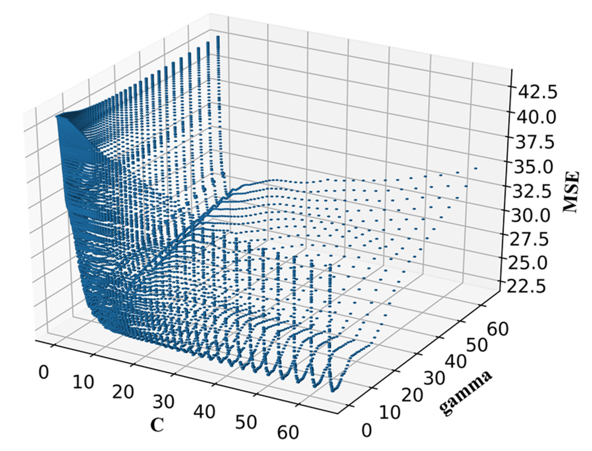
For the support vector regression model, the MSE of models with different C and gamma are shown in Figure 12. When C is 25.4 and gamma is 21.2, the gendered SVR model, referred to as SVR-M, achieves the smallest MSE.
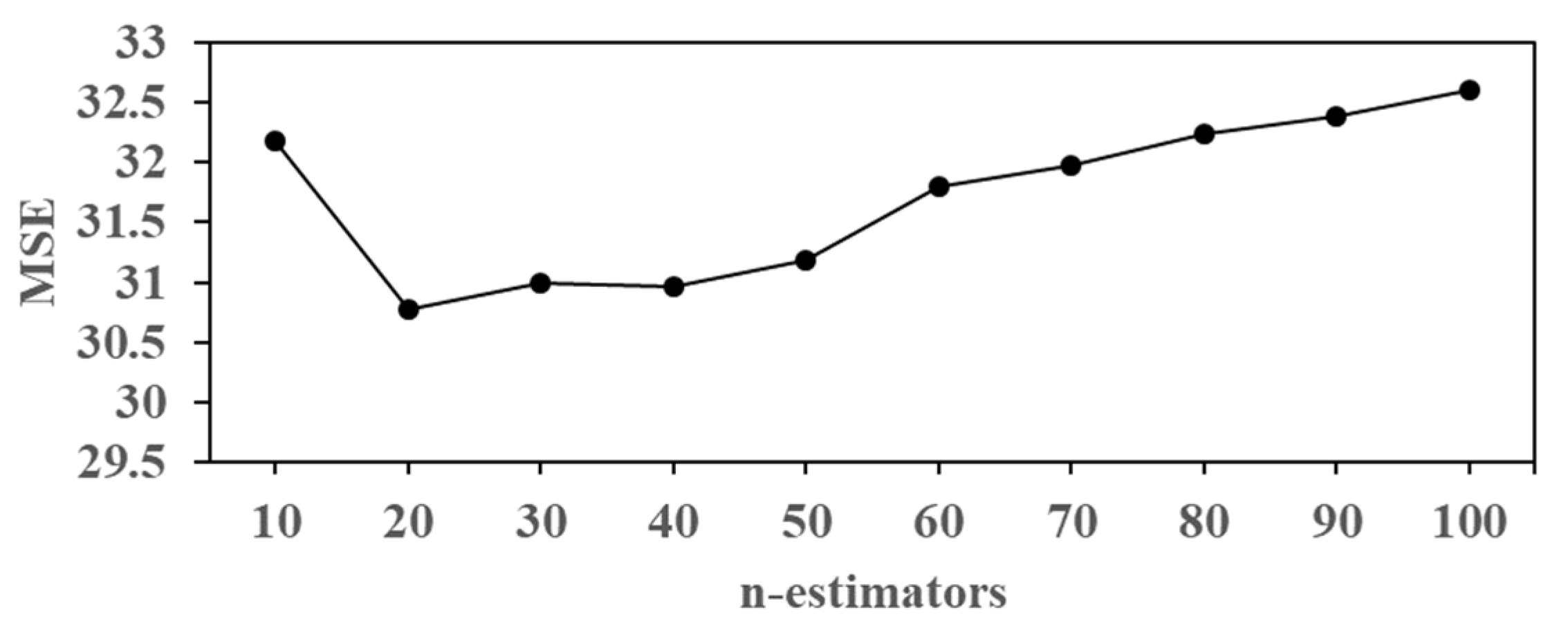
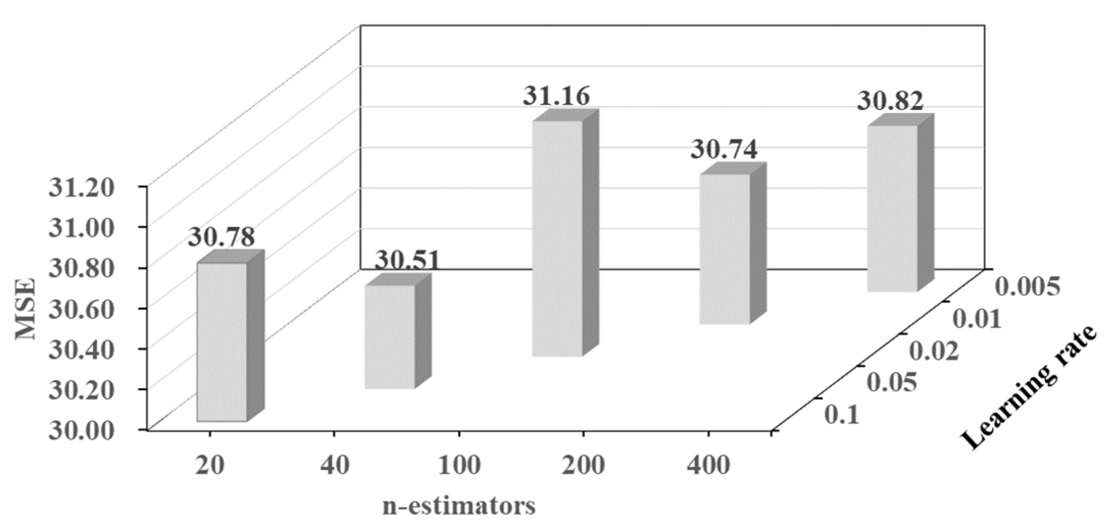
For the gradient boosting regression tree model, the number of features during establishing sub-decision tree, the max depth of sub-decision trees, the minimum number of samples for leaf nodes and other parameters use the default values from “sklearn.ensemble GradientBoostingRegressor.” of the Python toolkit: scikit-learn 0.22. The learning rate was initialized to an empirical value of 0.1. The number of sub-decision trees, marked as n-estimators, was optimized by GS-CV, and the MSE of models with different n-estimators is shown in Figure 13. According to Figure 13, when the n-estimators is 20, the generated GBRT model gets the smallest MSE. Since the parameter learning rate can also affect the performance of the GBRT model along with n-estimators, after getting an appropriate n-estimator the two parameters, n-estimator and learning rate, need to be tuned together. Meanwhile, the product of n-estimator and learning rate should not change. Therefore, several groups of parameter values were used to tune the performance of the GBRT model, and the MSE of models with different groups of parameters are shown in Figure 14. According to Figure 14, when the n-estimator is 40 and the learning rate is 0.05, the generated gradient boosting regression tree model(GBRT-M) gets the smallest MSE.

4.3. Performance of Four Machine Learning Algorithoms

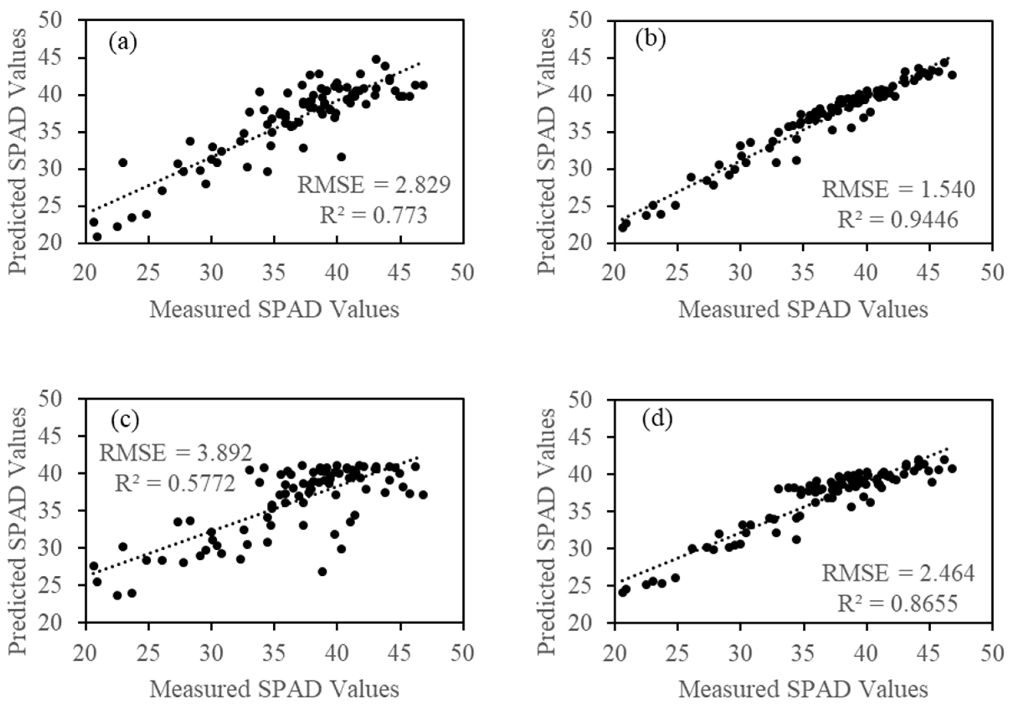
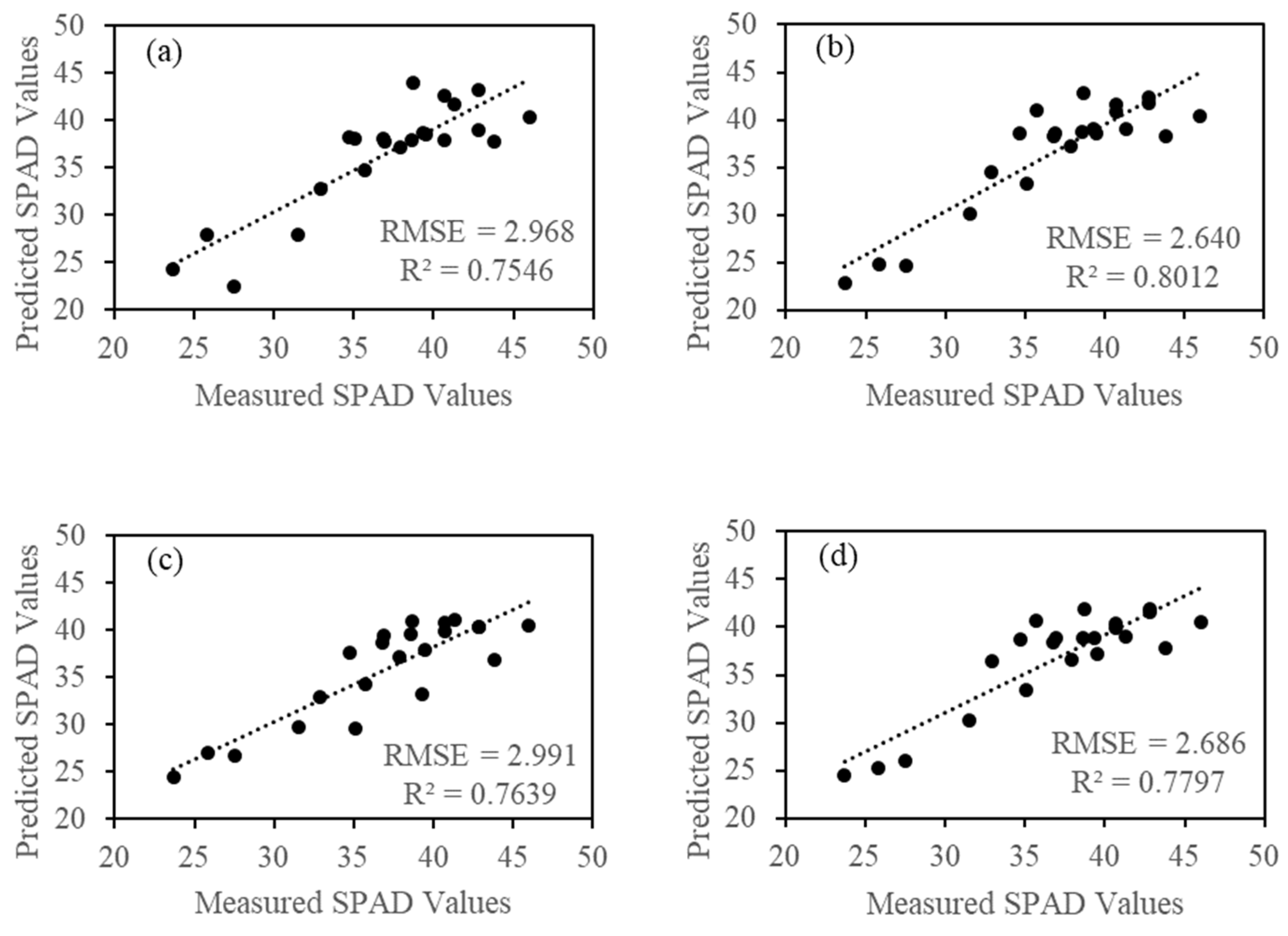
In this study, the optimal parameters of four machine learning algorithms for estimating rice SPAD were determined by GS-CV. To compare and assess the performance of the four generated machine learning models, training set, validation set and selected parameters were used. The final training and validating results of the four generated machine learning models, GPR-M, RFR-M, SVR-M, and GBRT-M, are shown in Table 3, Figure 15 and Figure 16.
It can be seen in Table 3 and Figure 15 that only three models, GPR-M, RFR-M, and GBR-M had an acceptable goodness-of-fit to the training set. The highest fit was achieved by the RFR-M (the RMSE, MAE, and R2 are 1.54, 1.23 and 0.95, respectively), followed by GBR-M (the RMSE, MAE, and R2 are 2.46, 2.02 and 0.87, respectively) and GPR-M (the RMSE, MAE and R2 are 2.83, 2.16 and 0.77, respectively). In contrast to the three models, SVR-M had the worst fit using the training set, the RMSE, MAE, and R2 are 3.89, 2.78, and 0.58, respectively.
Regarding the validating results (shown in Table 3 and Figure 16), the RFR-M had the highest prediction performance (RMSE = 2.64, MAE = 1.99 and R2 = 0.80), followed by the GBRT-M (RMSE = 2.69, MAE = 2.11 and R2 = 0.78). The differences between the performance of GPR-M (RMSE= 2.97, MAE = 2.30 and R2 = 0.76) and SVR-M (RMSE= 2.99, MAE = 2.23 and R2 = 0.76) is small, but both of them are slightly worse than the validation result of GBRT-M.
Previous studies have developed some vegetation indices to examine the chlorophyll content of plants (see Table 2). In addition, the correlation between the spectra’s first derivative and SPAD value was calculated and the spectra’s first derivative at 556.9 nm (labeled as FD556.9) had the strongest correlation with SPAD value. To further investigate the potential of the selected four RCRWa-b in estimating the SPAD value of rice, the predicted results (see in Table 4) of these vegetation indices and FD556.9 were obtained based on four machine learning algorithms and GS-CV. According to Table 4, four selected RCRWa-b generated higher accuracy than these vegetation indexes and FD556.9.

4.4. Changes of Rice Chlorophyll content during growing periods

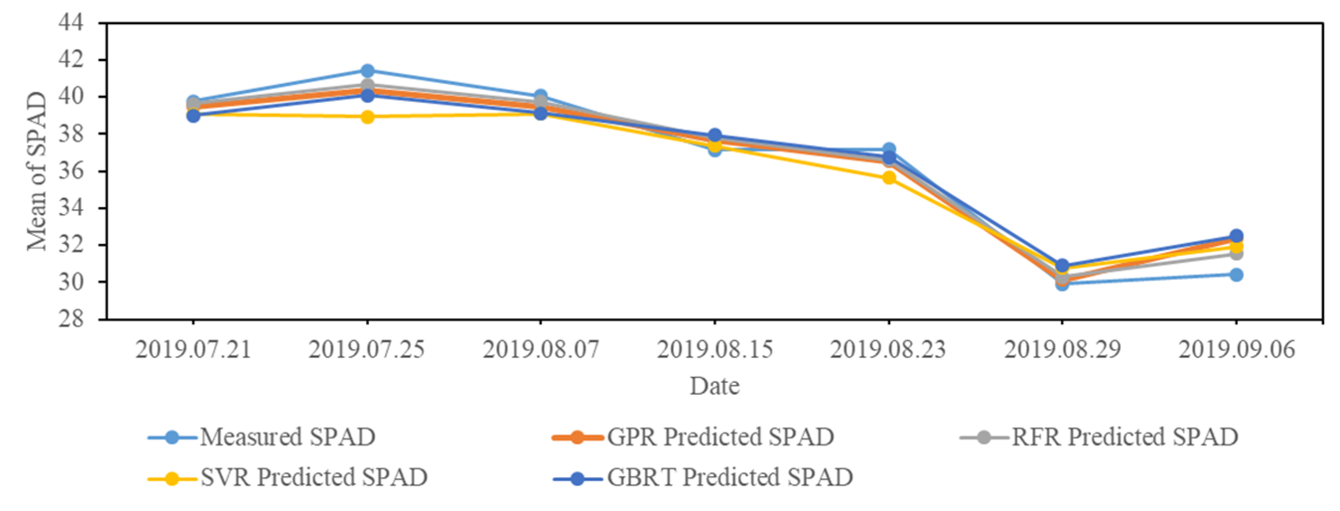
There were five sample plots on July 12, and 15 sample plots on all other dates. To improve the standardization, only the SPAD values collected from 21 July 2019 to 6 September 2019 were considered. Figure 17 shows how the mean of SPAD value (15 sample plots) change during these growing periods. According to Figure 17, the mean of the SPAD value first rose and then decreased.

5. Discussion

There have been, in the literature, many studies on estimating the chlorophyll content of the rice plant using machine learning methods. However, few studies have compared the performance of various machine learning algorithms in estimating the chlorophyll content of rice. In addition, the parameter optimization process of machine learning has been described in detail in a few studies. In this study, four machine learning models, GPR-M, RFR-M, SVR-M, and GBRT-M, were optimized and established based on in situ hyperspectral data and GS-CV parameter optimization algorithms. In addition, the performances of RCRWa-b, first derivative of spectra, and some indices for rice chlorophyll content estimation were compared. According to the selected features and the prediction results, the following outcomes were observed.
The RCRWa-b proposed in this study has apparent physical significance, which reflects the rate of change, either fast or slow, of reflectance between two wavelengths. There are redundant data between two RCRWa-b with adjacent ‘a’ or ‘b’ since collinearity exists between these two RCRWa-b. In this study, the RCRWa-b with the strongest correlation with SPAD value was selected from each wavelength range (four wavelength distribution ranges in total, see in Section 4.1) and four RCRWa-b were selected finally, which were RCRW551.0–565.6, RCRW739.5–743.5, RCRW684.4–687.1, and RCRW667.9–672. The performances of the four machine leaning techniques show that RCRWa-b is a potential variable for estimate the chlorophyll content of rice, and the predicted result indicates that these four features selected are effective to estimate the chlorophyll content of rice using machine learning algorithms.
Among the four generated machine learning models, the RFR-M yielded the highest accuracy in either the training set or validation set. However, the result of the training set is better than the result of the validation set, which indicates that the generalization of RFR-M is relatively poor. This may be due to the natural limitation of this algorithm, which often requires a relatively large data set, otherwise it could lead to an over-fitting problem [30].
The performance of the GBRT-M was the second best after RFR-M, and the performance characteristic of GBRT-M was similar to RFR-M, that is, although the GBRT-M showed an excellent goodness-of-fit, it provided relatively poor prediction results. However, in contrast to the RMSE and MAE of the results of RFR-M, the MAE of the training set and validation set of GBRT-M were very close, and the RMSE of the training set and validation set of GBRT-M were also very close. Therefore, compared to the RFR-M, the GBRT-M is more generalized and shows a stronger stability.
Regarding the SVR-M, this model had difficulties in learning from high SPAD values and lacked the sensibility to the high SPAD values, and the model showed under fitting, hence resulting in poor generalization, which mainly manifested in the R2 of predicted value using the training set is small and lower than the validation set, and the RMSE and MAE of predicted result of the training set were high, and higher than the validation set. The poor prediction using the training dataset and the large difference between the performance of the training set and the performance of the validation could be attributed to the fact that: (1) the parameters (C and gamma) selected by CV-GS are not optimal; (2) SVR has low potential to estimate SPAD values of rice by using the variable of RCRWa-b; or (3) both (1) and (2). Therefore, new machine learning parameter optimization algorithms should be considered to find the optimized values of the two parameters or new variable need be developed when using SVR algorithm for estimating the SPAD values of rice.
For the GPR-M, this model shows great generalization and robustness in estimating the SPAD value of rice by using four selected RCRWa-b when the data set is not large enough, which is mainly manifested in the R2, MAE, and RMSE of the predicted result for the training set being close to the R2, MAE, and RMSE of the predicted result for the validation set, respectively. Besides, although the performance of GPR-M is not the best, it is very close to the best one. Overall, GPR is a powerful machine leaning technique in estimating the SPAD value of rice.
By comparing the predicted results of Four-RCRWa-b, FD556.9 and some vegetation indices based on four machine learning algorithms (see Table 4), we found that: (1) no matter which algorithm is used, CI-green gives the worst result; (2) Four-RCRWa-b, FD556.9, MTCI and Re-NDVI show similar performance when using GPR; (3) the R2 of FD556.9 and Four-RCRWa-b are similar when using SVR, but the RMSE of the two show a relatively large difference; and (4) comparing with vegetation indices and FD556.9, Four-RCRWa-b gives the best results when using RFR, SVR, or GBRT. Therefore, when comparing with FD556.9 and certain vegetation indices, Four-RCRWa-b shows greater potential in estimating rice chlorophyll content, which is likely because Four-RCRWa-b considers more including the green, red, and red edge bands that are more chlorophyll sensitive.
Given the potential of Four-RCRWa-b in estimating rice chlorophyll content, its application to satellite data faces a big challenge because of the coarser spectral resolution of satellite sensors. The method is expected to work well when applying to unmanned aerial vehicle (UAV)-based hyperspectral imagery.
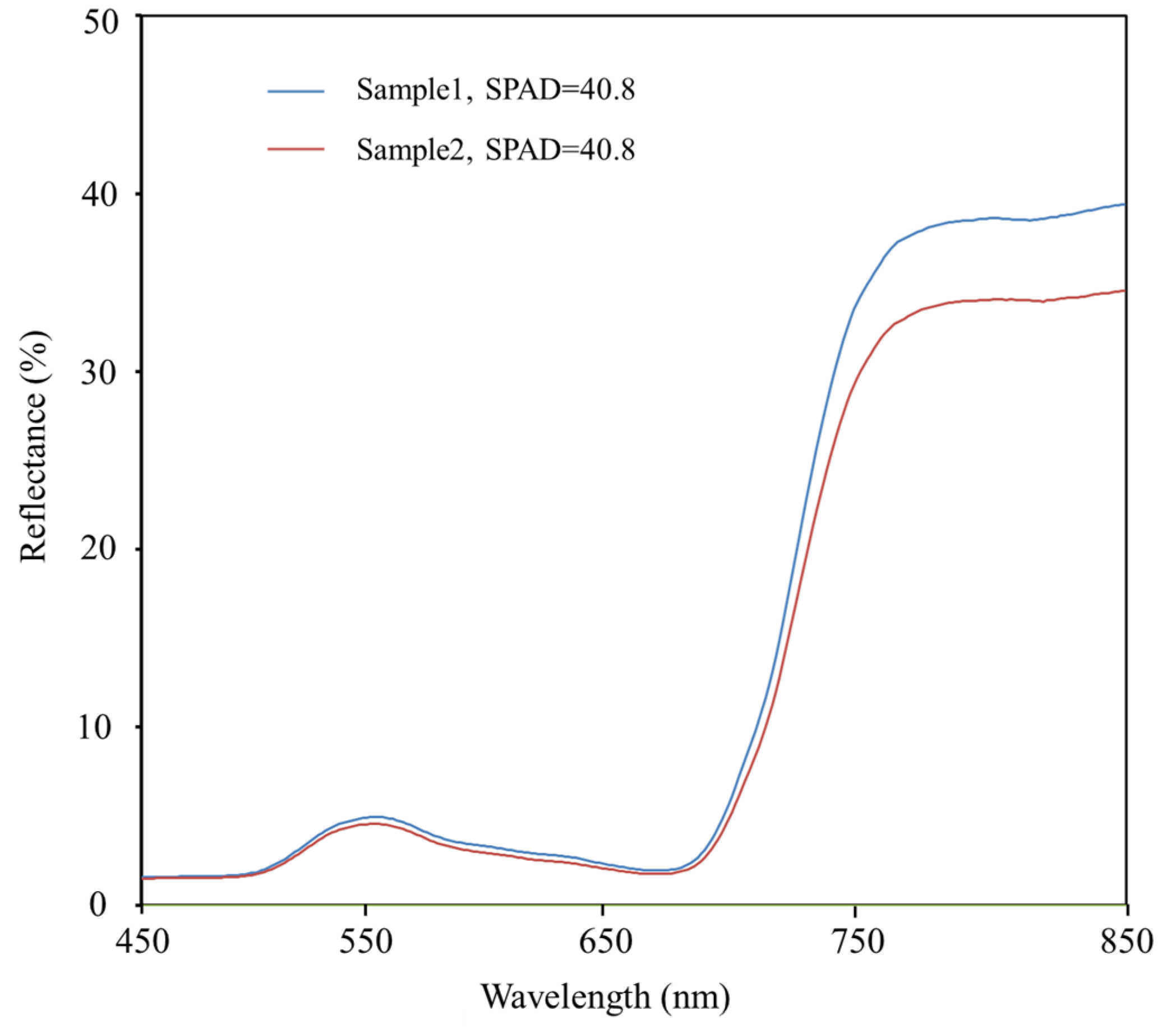
As the spectra measurements were performed on sunny clear days between 11:30 a.m. and 2:00 p.m., there may be some minor BRDF effects caused by the change of sunlight direction. Therefore, two sample plots (measured in different time) with the same SPAD value on 21 July 2019 (labeled as Sample1 and Sample2, and the solar altitude angle of Sample1 is greater than Sample2) were selected to investigate the influence of the BRDF effects caused by the change of sunlight direction on SPAD estimation. The spectra of Sample1 and Sample2 are shown in Figure 18. When the solar altitude angle was large, the reflectance in the near-infrared bands showed a significant increase than in visible bands. In addition, the RCRWa-b of Sample1 and Sample2 are also compared (Table 5). As shown in Table 5, when the solar altitude angle increased, the positive RCRWa-b values slightly increased, and the negative values slightly decreased. Table 6 shows the predicted results of Sample1 and Sample2 based on four generated machine learning methods. As seen in Table 6, the difference in predicted results between Sample1 and Sample2 is small. Therefore, we conclude that between 11:30 a.m. and 2:00 p.m., the BRDF effect caused by the change of solar altitude angle has little influence on SPAD estimation.

6. Conclusions and Recommendations

This study investigated the potential of RCRWa-b for estimating the chlorophyll content of rice plants using in situ hyperspectral data. Results of four advanced machine learning methods, including GPR, RFR, SVR, and GBRT, were investigated and compared. Based on the findings in this study, we conclude that:
  • The RCRWa-b has high potential in the estimation of the rice chlorophyll content.
  • RCRW551–565.6, RCRW739.5–743.5, RCRW684.4–687.1, and RCRW667.9–672 are effective features for estimating the rice chlorophyll content.
  • Compared to FD556.9 and some vegetation indices (MTCI, Re-NDVI, CI-green), Four-RCRWa-b generated better results.
  • Among the four machine learning techniques, GPR-M, RFR-M, SVR-M, and GBRT-M, RFR-M showed the best accuracy, and GPR-M showed the best generalization in estimating the chlorophyll content of rice.
Given the encouraging results from this study, limitations exist and should be addressed in future research. The field measurements cover only a portion of the rice growing period. In future studies, chlorophyll measurements covering the whole growing season should be collected and analyzed to evaluate the validity range of the proposed method. Furthermore, the method should be tested on other crop types to see if it will produce the same results.

Author Contributions

Data curation, G.A. and H.K.; Investigation, G.A., and M.X.; Methodology, M.X. and G.A; Supervision, B.H.; Validation, G.A. and M.X.; Writing—original draft, G.A. and M.X.; Writing—review & editing, G.A., M.X., B.H., C.L., J.S., X.H., and H.K. All authors have read and agreed to the published version of the manuscript.

Funding

This work was supported by the National Key R&D Program of China, grant number 2018YFD0200301; Sichuan Science and Technology Program, grant number 2020YFG0048;National Natural Science Foundation of China, grant number 41601373; the Open Fund of State Key Laboratory of Remote Sensing Science, grant number OFSLRSS201712; the Fundamental Research Funds for the Central Universities, grant number ZYGX2019J070; Department of Science and Technology of Sichuan Province, grant number 2020YFS0058.

Acknowledgments

The authors would like to appreciate Hongguo Zhang, Chunquan Fan, Shilei Feng, Yongqin Zhang, Yanxi Li, and Hao Tu in Quantitative remote sensing team at University of Electronic Science and Technology of China for their help of the data collection.

Conflicts of Interest

The authors declare no conflict of interest.

References

  1. Deng, L.; Mao, Z.; Li, X.; Hu, Z.; Duan, F.; Yan, Y. UAV-based multispectral remote sensing for precision agriculture: A comparison between different cameras. ISPRS J. Photogramm. Remote Sens. 2018, 146, 124–136. [Google Scholar] [CrossRef]
  2. Xu, X.; Lu, J.; Zhang, N.; Yang, T.; He, J.; Yao, X.; Cheng, T.; Zhu, Y.; Cao, W.; Tian, Y. Inversion of rice canopy chlorophyll content and leaf area index based on coupling of radiative transfer and Bayesian network models. ISPRS J. Photogramm. Remote Sens. 2019, 150, 185–196. [Google Scholar] [CrossRef]
  3. Moharana, S.; Dutta, S. Spatial variability of chlorophyll and nitrogen content of rice from hyperspectral imagery. ISPRS J. Photogramm. Remote Sens. 2016, 122, 17–29. [Google Scholar] [CrossRef]
  4. Gitelson, A.A.; Gritz, Y.; Merzlyak, M.N. Relationships between leaf chlorophyll content and spectral reflectance and algorithms for non-destructive chlorophyll assessment in higher plant leaves. J. Plant Physiol. 2003, 160, 271–282. [Google Scholar] [CrossRef]
  5. Darvishzadeh, R.; Skidmore, A.; Schlerf, M.; Atzberger, C.; Corsi, F.; Cho, M. LAI and chlorophyll estimation for a heterogeneous grassland using hyperspectral measurements. ISPRS J. Photogramm. Remote Sens. 2008, 63, 409–426. [Google Scholar] [CrossRef]
  6. Song, S.; Gong, W.; Zhu, B.; Huang, X. Wavelength selection and spectral discrimination for paddy rice, with laboratory measurements of hyperspectral leaf reflectance. ISPRS J. Photogramm. Remote Sens. 2011, 66, 672–682. [Google Scholar] [CrossRef]
  7. Li, L.; Ren, T.; Ma, Y.; Wei, Q.; Wang, S.; Li, X.; Cong, R.; Liu, S.; Lu, J. Evaluating chlorophyll density in winter oilseed rape (Brassica napus L.) using canopy hyperspectral red-edge parameters. Comput. Electron. Agric. 2016, 126, 21–31. [Google Scholar] [CrossRef]
  8. Hansen, P.; Schjoerring, J. Reflectance measurement of canopy biomass and nitrogen status in wheat crops using normalized difference vegetation indices and partial least squares regression. Remote Sens. Environ. 2003, 86, 542–553. [Google Scholar] [CrossRef]
  9. Le Maire, G.; Francois, C.; Dufrene, E. Towards universal broad leaf chlorophyll indices using PROSPECT simulated database and hyperspectral reflectance measurements. Remote Sens. Environ. 2004, 89, 1–28. [Google Scholar] [CrossRef]
  10. Dash, J.; Curran, P. The MERIS terrestrial chlorophyll index. Int. J. Remote Sens. 2004, 25, 5403–5413. [Google Scholar] [CrossRef]
  11. Delegido, J.; Alonso, L.; González, G.; Moreno, J. Estimating chlorophyll content of crops from hyperspectral data using a normalized area over reflectance curve (NAOC). Int. J. Appl. Earth Obs. Geoinf. 2010, 12, 165–174. [Google Scholar] [CrossRef]
  12. Xue, L.; Yang, L. Deriving leaf chlorophyll content of green-leafy vegetables from hyperspectral reflectance. ISPRS J. Photogramm. Remote Sens. 2009, 64, 97–106. [Google Scholar] [CrossRef]
  13. Liu, B.; Yue, Y.-M.; Li, R.; Shen, W.-J.; Wang, K.-L. Plant leaf chlorophyll content retrieval based on a field imaging spectroscopy system. Sensors 2014, 14, 19910–19925. [Google Scholar] [CrossRef] [PubMed] [Green Version]
  14. Van Cleemput, E.; Vanierschot, L.; Fernández-Castilla, B.; Honnay, O.; Somers, B. The functional characterization of grass-and shrubland ecosystems using hyperspectral remote sensing: Trends, accuracy and moderating variables. Remote Sens. Environ. 2018, 209, 747–763. [Google Scholar] [CrossRef]
  15. Verrelst, J.; Camps-Valls, G.; Muñoz-Marí, J.; Rivera, J.P.; Veroustraete, F.; Clevers, J.G.; Moreno, J. Optical remote sensing and the retrieval of terrestrial vegetation bio-geophysical properties–A review. ISPRS J. Photogramm. Remote Sens. 2015, 108, 273–290. [Google Scholar] [CrossRef]
  16. Casa, R.; Jones, H. Retrieval of crop canopy properties: A comparison between model inversion from hyperspectral data and image classification. Int. J. Remote Sens. 2004, 25, 1119–1130. [Google Scholar] [CrossRef]
  17. Li, Z.; Jin, X.; Yang, G.; Drummond, J.; Yang, H.; Clark, B.; Li, Z.; Zhao, C. Remote sensing of leaf and canopy nitrogen status in winter wheat (Triticum aestivum L.) based on N-PROSAIL model. Remote Sens. 2018, 10, 1463. [Google Scholar] [CrossRef] [Green Version]
  18. Marshall, M.; Thenkabail, P. Advantage of hyperspectral EO-1 Hyperion over multispectral IKONOS, GeoEye-1, WorldView-2, Landsat ETM+, and MODIS vegetation indices in crop biomass estimation. ISPRS J. Photogramm. Remote Sens. 2015, 108, 205–218. [Google Scholar] [CrossRef] [Green Version]
  19. Cavallo, D.P.; Cefola, M.; Pace, B.; Logrieco, A.F.; Attolico, G. Contactless and non-destructive chlorophyll content prediction by random forest regression: A case study on fresh-cut rocket leaves. Comput. Electron. Agric. 2017, 140, 303–310. [Google Scholar] [CrossRef]
  20. Yang, X.; Huang, J.; Wu, Y.; Wang, J.; Wang, P.; Wang, X.; Huete, A.R. Estimating biophysical parameters of rice with remote sensing data using support vector machines. Sci. China Life Sci. 2011, 54, 272–281. [Google Scholar] [CrossRef] [Green Version]
  21. Liu, H.; Li, M.; Zhang, J.; Gao, D.; Sun, H.; Yang, L. Estimation of chlorophyll content in maize canopy using wavelet denoising and SVR method. Int. J. Agric. Biol. Eng. 2018, 11, 132–137. [Google Scholar] [CrossRef] [Green Version]
  22. Kalacska, M.; Lalonde, M.; Moore, T. Estimation of foliar chlorophyll and nitrogen content in an ombrotrophic bog from hyperspectral data: Scaling from leaf to image. Remote Sens. Environ. 2015, 169, 270–279. [Google Scholar] [CrossRef]
  23. Delloye, C.; Weiss, M.; Defourny, P. Retrieval of the canopy chlorophyll content from Sentinel-2 spectral bands to estimate nitrogen uptake in intensive winter wheat cropping systems. Remote Sens. Environ. 2018, 216, 245–261. [Google Scholar] [CrossRef]
  24. Verrelst, J.; Alonso, L.; Camps-Valls, G.; Delegido, J.; Moreno, J. Retrieval of vegetation biophysical parameters using Gaussian process techniques. IEEE Trans. Geosci. Remote Sens. 2011, 50, 1832–1843. [Google Scholar] [CrossRef]
  25. Paul, S.; Poliyapram, V.; İmamoğlu, N.; Uto, K.; Nakamura, R.; Kumar, D.N. Canopy Averaged Chlorophyll Content Prediction of Pear Trees Using Convolutional Autoencoder on Hyperspectral Data. IEEE J. Sel. Top. Appl. Earth Obs. Remote Sens. 2020, 13, 1426–1437. [Google Scholar] [CrossRef]
  26. Markwell, J.; Osterman, J.C.; Mitchell, J.L. Calibration of the Minolta SPAD-502 leaf chlorophyll meter. Photosynth. Res. 1995, 46, 467–472. [Google Scholar] [CrossRef]
  27. Yang, W.-H.; Peng, S.; Huang, J.; Sanico, A.L.; Buresh, R.J.; Witt, C. Using leaf color charts to estimate leaf nitrogen status of rice. Agron. J. 2003, 95, 212–217. [Google Scholar]
  28. Vos, J.; Bom, M. Hand-held chlorophyll meter: A promising tool to assess the nitrogen status of potato foliage. Potato Res. 1993, 36, 301–308. [Google Scholar] [CrossRef]
  29. Fassnacht, F.E.; Hartig, F.; Latifi, H.; Berger, C.; Hernández, J.; Corvalán, P.; Koch, B. Importance of sample size, data type and prediction method for remote sensing-based estimations of aboveground forest biomass. Remote Sens. Environ. 2014, 154, 102–114. [Google Scholar] [CrossRef]
  30. Hoa, P.V.; Giang, N.V.; Binh, N.A.; Hai, L.V.H.; Pham, T.-D.; Hasanlou, M.; Tien Bui, D. Soil salinity mapping using SAR sentinel-1 data and advanced machine learning algorithms: A case study at Ben Tre Province of the Mekong River Delta (Vietnam). Remote Sens. 2019, 11, 128. [Google Scholar] [CrossRef] [Green Version]
  31. Vafaei, S.; Soosani, J.; Adeli, K.; Fadaei, H.; Naghavi, H.; Pham, T.D.; Tien Bui, D. Improving accuracy estimation of Forest Aboveground Biomass based on incorporation of ALOS-2 PALSAR-2 and Sentinel-2A imagery and machine learning: A case study of the Hyrcanian forest area (Iran). Remote Sens. 2018, 10, 172. [Google Scholar] [CrossRef] [Green Version]
  32. Rasmussen, C.E. Gaussian processes in machine learning. In Summer School on Machine Learning; Springer: Berlin/Heidelberg, Germany, 2003; pp. 63–71. [Google Scholar]
  33. Singhal, G.; Bansod, B.; Mathew, L.; Goswami, J.; Choudhury, B.; Raju, P. Chlorophyll estimation using multi-spectral unmanned aerial system based on machine learning techniques. Remote Sens. Appl. Soc. Environ. 2019, 15, 100235. [Google Scholar] [CrossRef]
  34. Breiman, L. Random forests. Mach. Learn. 2001, 45, 5–32. [Google Scholar] [CrossRef] [Green Version]
  35. Wu, X.; Kumar, V.; Quinlan, J.R.; Ghosh, J.; Yang, Q.; Motoda, H.; Mclachlan, G.J.; Ng, A.S.K.; Liu, B.; Yu, P.S. Top 10 algorithms in data mining. Knowl. Inf. Syst. 2007, 14, 1–37. [Google Scholar] [CrossRef] [Green Version]
  36. Mountrakis, G.; Im, J.; Ogole, C. Support vector machines in remote sensing: A review. ISPRS J. Photogramm. Remote Sens. 2011, 66, 247–259. [Google Scholar] [CrossRef]
  37. Sun, J.; Yang, J.; Shi, S.; Chen, B.; Du, L.; Gong, W.; Song, S. Estimating rice leaf nitrogen concentration: Influence of regression algorithms based on passive and active leaf reflectance. Remote Sens. 2017, 9, 951. [Google Scholar] [CrossRef] [Green Version]
  38. Wei, L.; Yuan, Z.; Zhong, Y.; Yang, L.; Hu, X.; Zhang, Y. An Improved Gradient Boosting Regression Tree Estimation Model for Soil Heavy Metal (Arsenic) Pollution Monitoring Using Hyperspectral Remote Sensing. Appl. Sci. 2019, 9, 1943. [Google Scholar] [CrossRef] [Green Version]
  39. Wang, S.; Chen, Y.; Wang, M.; Li, J. Performance Comparison of Machine Learning Algorithms for Estimating the Soil Salinity of Salt-Affected Soil Using Field Spectral Data. Remote Sens. 2019, 11, 2605. [Google Scholar] [CrossRef] [Green Version]
  40. Chai, T.; Draxler, R.R. Root mean square error (RMSE) or mean absolute error (MAE)?–Arguments against avoiding RMSE in the literature. Geosci. Model Dev. 2014, 7, 1247–1250. [Google Scholar] [CrossRef] [Green Version]
  41. Barnes, E.; Clarke, T.; Richards, S.; Colaizzi, P.; Haberland, J.; Kostrzewski, M.; Waller, P.; Choi, C.; Riley, E.; Thompson, T. Coincident detection of crop water stress, nitrogen status and canopy density using ground based multispectral data. In Proceedings of the Fifth International Conference on Precision Agriculture, Bloomington, MN, USA, 16–19 July 2000. [Google Scholar]
  42. Gitelson, A.A.; Keydan, G.P.; Merzlyak, M.N. Three-band model for noninvasive estimation of chlorophyll, carotenoids, and anthocyanin contents in higher plant leaves. Geophys. Res. Lett. 2006, 33. [Google Scholar] [CrossRef] [Green Version]
  43. Gitelson, A.A.; Buschmann, C.; Lichtenthaler, H.K. The chlorophyll fluorescence ratio F735/F700 as an accurate measure of the chlorophyll content in plants. Remote Sens. Environ. 1999, 69, 296–302. [Google Scholar] [CrossRef]
  44. Zarco-Tejada, P.J.; Miller, J.R.; Noland, T.L.; Mohammed, G.H.; Sampson, P.H. Scaling-up and model inversion methods with narrowband optical indices for chlorophyll content estimation in closed forest canopies with hyperspectral data. IEEE Trans. Geosci. Remote Sens. 2001, 39, 1491–1507. [Google Scholar] [CrossRef] [Green Version]
  45. Tian, Y.; Yao, X.; Yang, J.; Cao, W.; Hannaway, D.; Zhu, Y. Assessing newly developed and published vegetation indices for estimating rice leaf nitrogen concentration with ground-and space-based hyperspectral reflectance. Field Crops Res. 2011, 120, 299–310. [Google Scholar] [CrossRef]
  46. Blackburn, G.A. Spectral indices for estimating photosynthetic pigment concentrations: A test using senescent tree leaves. Int. J. Remote Sens. 1998, 19, 657–675. [Google Scholar] [CrossRef]
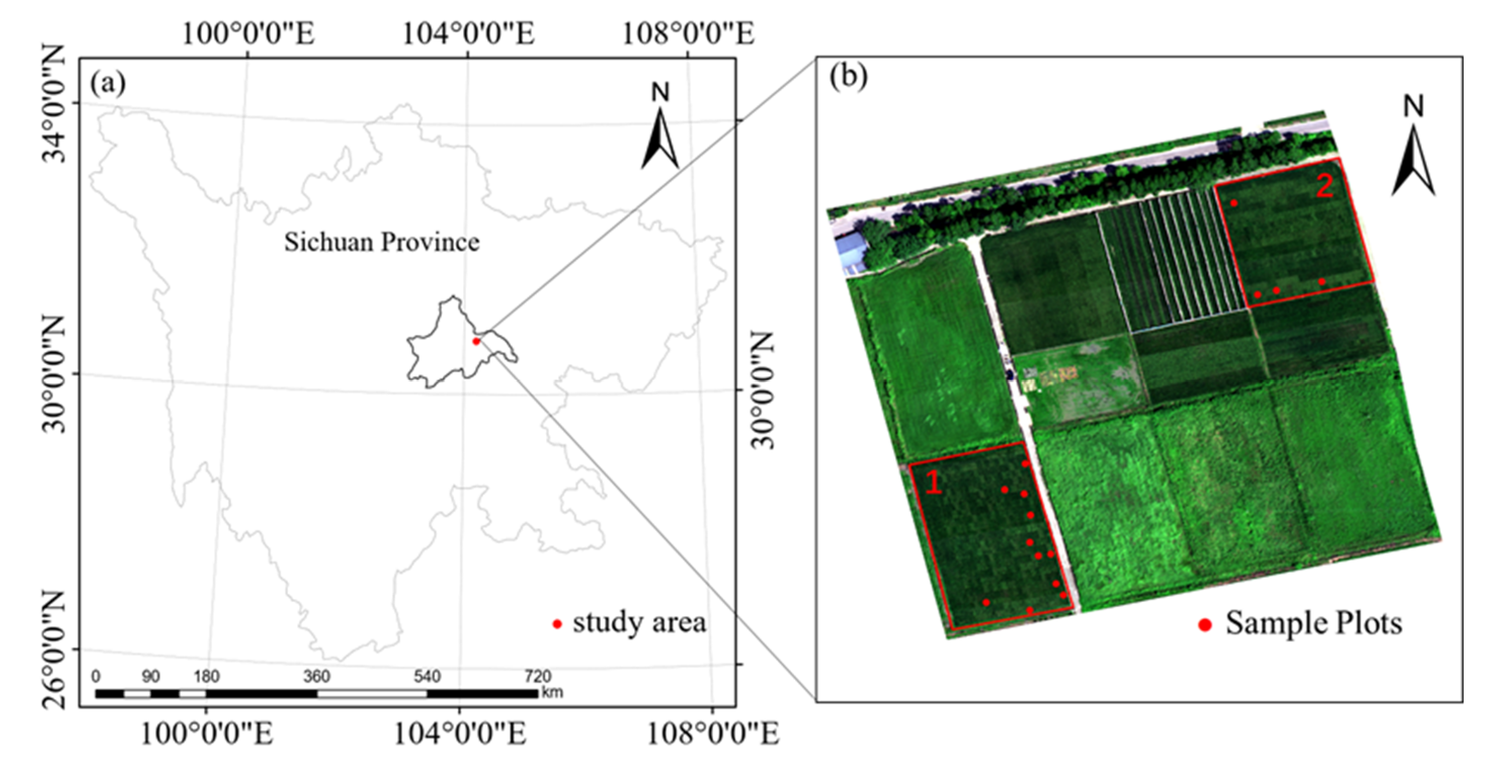
Figure 1. (a) Location of the field experimental site. (b) The spatial distribution of sample plots.
Remotesensing 12 03104 g001
Figure 2. The straight line obtained by linear fitting the reflectance value and the corresponding wavelengths.
Remotesensing 12 03104 g002
Figure 3. Proposed workflow for this study.
Remotesensing 12 03104 g003
Figure 4. The measured spectra of rice plants between 450 nm and 850 nm.
Remotesensing 12 03104 g004
Figure 5. Correlogram between rate of change in reflectance between wavelengths ‘a’ and ‘b’ (RCRWa-b) and soil–plant analysis development (SPAD) value.
Remotesensing 12 03104 g005
Figure 6. (a) The reflectance and wavelength corresponding to RCRW520–640; (b) the reflectance and wavelength corresponding to RCRW600–700.
Remotesensing 12 03104 g006
Figure 7. The range of wavelength ‘a’ and ‘b’ under some restrictions.
Remotesensing 12 03104 g007
Figure 8. (a) The correlation coefficient between RCRW536.3–543.7 and RCRW540.7–549.5; (b) the correlation coefficient between RCRW658.2–665.1 and RCRW662.3–670.6.
Remotesensing 12 03104 g008
Figure 9. Scatter plots between (a) SPAD and RCRW551.0–565.6, (b) SPAD and RCRW739.5–743.5, (c) SPAD and RCRW684.4–687.1, (d) SPAD and RCRW667.9–672.0.
Remotesensing 12 03104 g009
Figure 10. The statistics characteristics of dataset.
Remotesensing 12 03104 g010
Figure 11. The mean square error (MSE) of random forest regression model of different n-estimator. Note: the range of n-estimator is from 10 to 300 and the step length is 10.
Remotesensing 12 03104 g011
Figure 12. The MSE of the support vector regression (SVR)model with different C and gamma. Note: The range of parameter C is from 2M to 2N and M is −6, N is 6 and the step length between M and N is 0.1; The range of parameter gamma is from 2M to 2N and M is −6, N is 6 and the step length between M and N is 0.1;.
Remotesensing 12 03104 g012
Figure 13. The MSE of gradient boosting regression tree model(GBRT-M) with different n-estimators. Note: the range of n-estimators is from 10 to 100, and the step length is 10.
Remotesensing 12 03104 g013
Figure 14. The MSE of the GBRT-M with different n-estimators and learning rate.
Remotesensing 12 03104 g014
Figure 15. Scatterplots between the measured SPAD value and the predicted SPAD value using the training set. Note: (a) GPR-M; (b) RFR-M; (c) SVR-M; (d) GBRT-M.
Remotesensing 12 03104 g015
Figure 16. Scatterplots between the measured SPAD value and the predicted SPAD value using the validation set. Note: (a) GPR-M; (b) RFR-M; (c) SVR-M; (d) GBRT-M.
Remotesensing 12 03104 g016
Figure 17. Dynamics of mean of SPAD value during July 21 to 6 September 2019.
Remotesensing 12 03104 g017
Figure 18. The spectra of Sample1 and Sample2.
Remotesensing 12 03104 g018
Table 1. Dates of measuring and the number of sample plots.
Date of MeasuringThe Number of Sample Plots in Field1The Number of Sample Plots in Field2The Total Number of Sample Plots
12 July 2019505
21 July 201911415
25 July 201911415
7 August 201911415
15 August 201911415
23 August 201911415
29 August 201911415
6 September 201911415
Table 2. Vegetation indices examined for chlorophyll content estimation.
IndexEquationReference
MTCI R 753.75 R 708.75 R 708.75 R 681.25 [10]
RE-NDVI R 790 R 720 R 790 + R 720 [41]
CI-green R 780 R 550 1 [42]
Table 3. Performance of the four machine learning models using the training set and validation set.
SPAD Estimation ModelTraining SetValidation Set
RMSEMAER2RMSEMAER2
Gaussian Process Regression Model (GPR-M)2.83 2.16 0.77 2.97 2.30 0.76
Random Forest Regression Model (RFR-M)1.54 1.26 0.95 2.64 1.99 0.80
Support Vector Regression Model (SVR-M)3.89 2.78 0.58 2.99 2.23 0.76
Gradient Boosting Regression Tree Model (GBRT-M)2.46 2.02 0.87 2.69 2.11 0.78
Table 4. Predicted results of some indexes using four machine learning algorithms and grid search-cross validation (GS-CV).
IndexMachine Learning AlgorithmsRMSEMAER2
Four-RCRWa-bGaussian Process Regression2.972.300.76
Random Forest Regression2.641.990.80
Support Vector Regression2.992.300.76
Gradient Boosting Regression Tree2.872.110.78
FD556.9Gaussian Process Regression2.701.890.77
Random Forest Regression3.943.550.60
Support Vector Regression3.402.640.76
Gradient Boosting Regression Tree3.112.500.71
MTCIGaussian Process Regression2.942.280.75
Random Forest Regression3.292.450.70
Support Vector Regression3.182.280.71
Gradient Boosting Regression Tree2.962.30.78
RE-NDVIGaussian Process Regression2.952.300.76
Random Forest Regression4.093.060.61
Support Vector Regression3.082.120.73
Gradient Boosting Regression Tree3.612.620.68
CI-greenGaussian Process Regression4.313.020.64
Random Forest Regression4.012.810.54
Support Vector Regression3.862.480.57
Gradient Boosting Regression Tree3.552.400.61
Table 5. The Four-RCRWa-b values of Sample1 and Sample2.
SampleRCRW551–565.6RCRW739.5–743.5RCRW684.4–687.1RCRW667.9–672
Sample1−0.0170.5780.079−0.007
Sample2−0.0160.5170.066−0.005
Table 6. The training results of Sample1 and Sample2 based on four generated machine leaning models.
SampleGPR-MRFR-MSVR-MGBRT-M
Sample139.3240.5040.6539.40
Sample241.0539.9740.7039.13