Abstract
L-band brightness temperature () is one of the key remotely-sensed variables that provides information regarding surface soil moisture conditions. In order to harness the information in observations, a radiative transfer model (RTM) is investigated for eventual inclusion into a data assimilation framework. In this study, estimates from the RTM implemented in the NASA Goddard Earth Observing System (GEOS) were evaluated against the nearly four-year record of daily observations collected by L-band radiometers onboard the Aquarius satellite. Statistics between the modeled and observed were computed over North America as a function of soil hydraulic properties and vegetation types. Overall, statistics showed good agreement between the modeled and observed with a relatively low, domain-average bias (0.79 K (ascending) and −2.79 K (descending)), root mean squared error (11.0 K (ascending) and 11.7 K (descending)), and unbiased root mean squared error (8.14 K (ascending) and 8.28 K (descending)). In terms of soil hydraulic parameters, large porosity and large wilting point both lead to high uncertainty in modeled due to the large variability in dielectric constant and surface roughness used by the RTM. The performance of the RTM as a function of vegetation type suggests better agreement in regions with broadleaf deciduous and needleleaf forests while grassland regions exhibited the worst accuracy amongst the five different vegetation types.
1. Introduction
Soil moisture is a crucial component in hydrologic, meteorologic, and land surface processes [1,2,3]. Soil moisture interacts with the overlying atmosphere via evapotranspiration and precipitation recycling [4,5] and plays a substantial role in the water and energy balances by acting as a first-order control on the partitioning of surface energy and precipitation fluxes [6,7,8,9,10,11,12,13]. In addition, soil moisture–precipitation feedback plays an important role in controlling weather patterns, which is evident particularly in transitional climate zones [5,14,15].
Soil moisture can be inferred from microwave (MW) measurements collected by passive microwave radiometers (typically provided as brightness temperature, ). The emitted from the Earth’s surface is a function of the physical temperature of the land surface times the land surface emissivity [16,17]. Microwave emissivity of soil is largely dependent on the dielectric constant of the soil, which is a strong function of the amount of water within the soil matrix [18,19]. The large contrast between the dielectric constant of water at L-band (about 80) and dry soil (about 3.5) results in a large difference between the emissivities from wet and dry soil (roughly 0.6 and 0.95, respectively) [20,21], which fundamentally forms the basis for passive microwave remote sensing of soil moisture.
Several space-based, L-band (1–2 GHz) microwave radiometers have been launched in the past decade in order to retrieve soil moisture. The European Space Agency launched the Soil Moisture Ocean Salinity (SMOS) mission in November 2009, which provides global retrievals of surface soil moisture over land and surface salinity over oceans with an approximate three-day repeat cycle [22,23,24]. The multi-angular, dual-polarized L-band radiometer on-board SMOS provides observations at a nominal horizontal resolution of 40 km with a soil moisture retrieval accuracy of 0.04 m3/m3 [24] yielding reasonable agreement with in-situ soil moisture observations [25,26,27,28,29]. The National Aeronautics and Space Administration (NASA) launched the Soil Moisture Active–Passive (SMAP) mission on 31 January 2015 in order to provide observations of surface soil moisture and freeze–thaw products with a spatial and temporal resolution of ∼40 km and ∼3 days, respectively [30]. The main difference between the SMOS and SMAP radiometers is that SMAP observes at a single incidence angle with increased accuracy and improved mitigation of radio frequency interference (RFI) whereas SMOS observes at multiple incidence angles.
The Aquarius mission, which was launched on 10 June 2011 and ended on 8 June 2015, also carries three L-band radiometers with its primary design objective to monitor sea surface salinity [31]. In general, observed from SMOS and Aquarius showed strong correlation and similar climatology over land [32,33]. Piepmeier et al. [33] compared the concurrent SMOS and Aquarius observations worldwide with SMOS observations rescaled into the incidence angles and footprints of Aquarius. Statistical comparison of Aquarius and SMOS revealed strong correlation (>0.97) over the land across the polarizations and incidence angles with a warmer bias (approximately 8 K and 6 K for horizontal and vertical polarization, respectively) for Aquarius compared to SMOS . Pablos et al. [32] also revealed a strong correlation between the Aquarius and SMOS observations with similar seasonal variation over land. However, the relatively coarse temporal and spatial resolution (i.e., seven-day revisit frequency and 390 of native spatial footprint) impose some limitations during the application of Aquarius in the estimation of soil moisture [34].
Recent studies have demonstrated the benefit of merging L-band with a land surface model in order to improve soil moisture estimates [35,36,37,38,39,40,41,42]. Such a merger typically involves a data assimilation (DA) system that uses a Radiative Transfer Model (RTM) to map the geophysical model states (e.g., soil moisture) into observation (i.e., ) space [43]. For instance, De Lannoy et al. [44] coupled a zero-order tau–omega model to the GEOS Catchment Land Surface Model (Catchment) in order to produce global estimates of L-band . Inputs to the GEOS RTM include variable estimates derived from the Catchment model [45]. The most sensitive parameters in the RTM were calibrated using SMOS observations [44].
The main objective of this study is to investigate the performance of the GEOS RTM through a comparison with observations collected by the Aquarius L-band radiometer over North America. More specifically, multi-year SMOS observations were utilized in the calibration of RTM parameters because SMOS provides a multi-year record of multi-angular observations with ∼2-day global repeat frequency at ∼40 km resolution. Further, the utilization of SMOS enables an independent evaluation of RTM-derived with Aquarius across the entire Aquarius observational record, as opposed to a direct comparison against SMOS , which is much more limited in spatio-temporal coverage owing to the limited number of common overpass times and locations. Even though the Aquarius mission ended in 2015, Aquarius observations are still valuable (along with SMAP and SMOS observations) to develop a long-term, L-band record, which is helpful to fill spatial or temporal gaps in the SMOS and SMAP records as well as improve the accuracy of observed through calibration with one another. Moreover, such comparisons will help improve the RTM-derived estimates, and hence, lead to potential improvements in soil moisture estimates using a data assimilation framework as part of a land surface reanalysis.
The performance of the RTM was investigated as a function of soil type and overlying vegetation type. Exploring the performance of the RTM as a function of soil hydraulic parameters (SHPs) and vegetation type helps better understand the RTM’s capability across different portions of the globe. An eventual goal in the future is to merge Aquarius observations and RTM-derived estimates within an ensemble-based data assimilation framework. However, prior to conducting L-band assimilation in a follow-on study, it is critical to first examine and evaluate the observation operator (i.e., the RTM) in order to assess its capabilities and error characteristics.
2. Microwave Radiative Transfer Theory
Microwave radiative transfer theory applied to soil moisture, in general, provides a framework to estimate at the top of the atmosphere, [46]. This consists of upward and downward atmospheric radiation along with surface and vegetation components. Here, we focus on the description of at the top of the vegetation, , as the Aquarius observations have already undergone atmospheric correction. The tau-omega model simplifies calculation at polarization as:
where [K] is the surface soil temperature, and [K] is the canopy temperature that is assumed to equal [44]. [-] is the rough surface soil reflectivity, [-] is the scattering albedo, and [-] is the vegetation attenuation.
Vegetation attenuation, , is calculated through the vegetation opacity model [47] as:
where [rad] is the incidence angle and is the vegetation opacity at nadir. is a function of the vegetation structure parameter, [-], and the vegetation water content, [kg m−2]. is calculated as the product of leaf equivalent water thickness, [kg m−2], and leaf area index, [m−2 m−2]. The rough surface reflectivity, , in Equation (1) is calculated as a function of smooth surface reflectivity, , via:
where Q [-] is the polarization mixing factor (assumed to be 0 for L-band) due to surface roughness, N [-] is the angular dependence, and q indicates polarizations when . h [-] is the effective roughness height parameterized as a stepwise function where:
where [m3 m−3] represents porosity and [m3 m−3] is the transitional soil moisture calculated as a function of wilting point [48]. The parameters and represent the roughness height when soil moisture is less than transitional soil moisture and at saturation, respectively. The smooth surface reflectivity, , is computed from the Fresnel equations, which is dependent on the soil dielectric constant that varies with soil moisture [49]. The dielectric constant formulation used in the RTM is based on Wang and Schmugge [48].
From Equation (1), the vegetation attenuates the microwave emission from the soil and simultaneously adds its own contribution to the measured microwave . In addition, precipitation interception by overlying vegetation and ground litter also affects microwave emission from the soil [50]. The RTM employed in this study neglects interception and littering effects [44]. Details on the calibration procedure of the GEOS RTM are found in Section 3.2.
3. Data and Methods
3.1. Aquarius Satellite Mission
The Aquarius instrument was part of the Aquarius/Satéllite de Aplicaciones Científicas (SAC-D) mission, which was launched on 10 June 2011 and ended on 8 June 2015 [31]. The mission is a joint collaboration between NASA and the Argentinian space agency, Comisión Nacional de Actividades Espaciales (CONAE), with participation from Brazil, Canada, France, and Italy. The Aquarius instrument is a combination of an active scatterometer and passive radiometers that measure L-band (1.4 GHz) radiation. The observations employed in this study are derived only from the passive radiometers.
Even though the Aquarius mission was launched with the main goal of measuring sea surface salinity, the L-band observations discussed here are used in the context of soil moisture remote sensing over non-frozen land. Three passive radiometers provide observations at a spatial resolution (i.e., approximate field-of-view) of , with incidence angles of , , and , respectively. These incidence angles are denoted by beam #1, beam #2, and beam #3, respectively. The minor axis of each beam is in the along-track direction while the major axis is aligned in the cross-track direction. Each radiometer is directed toward the night side of the Earth in order to avoid Sun glint. Aquarius is a sun-synchronous, polar-orbiting satellite with a global repeat interval of ∼7 days. Aquarius underwent pre-launch and post-launch calibration activities [33]. Pre-launch calibration included receiver and antenna switch-matrix calibration. Post-launch calibration included the correction of diode noise, antenna patterns, RFI, and cold-sky calibration [51]. Note that Aquarius observations were not calibrated to the SMOS observations.
Data provided by the Aquarius mission during the study period from 25 August 2011 to 7 June 2015 were obtained from the NASA Jet Propulsion Laboratory (JPL) in the Hierarchical Data Format (HDF5) at ftp://podaac.jpl.nasa.gov. Level-2, version-4 Aquarius data products used in this study provide observations for both ascending (∼6 a.m. local time) and descending (∼6 p.m. local time) overpasses at both horizontal and vertical polarizations.
3.2. GEOS Radiative Transfer Model Implementation
The GEOS RTM considers several variables (e.g., surface soil moisture, surface soil temperature, and vegetation water content) from the NASA Catchment Land Surface Model [45] for the purpose of calibration along with SMOS as well as producing RTM-derived . Among the various RTM parameters, microwave effective roughness height (h), scattering albedo (), and the vegetation structure parameter () were selected for calibration using multi-angular SMOS observations in order to compute estimates at the top of vegetation at both horizontal and vertical polarizations [37,38,44]. During the calibration using a particle swarm optimization search algorithm, the difference in the long-term temporal mean and temporal standard deviation of between SMOS and RTM were minimized, which helps minimize the climatological difference between the different datasets [44]. Where SMOS observations are unavailable for calibration, these RTM parameters were filled in by using an average of calibrated parameters for other regions with the same vegetation class. Uncalibrated RTM parameters (e.g., leaf equivalent water thickness (LEWT) and angular dependence ()) were assigned literature-based lookup table values associated with each vegetation class.
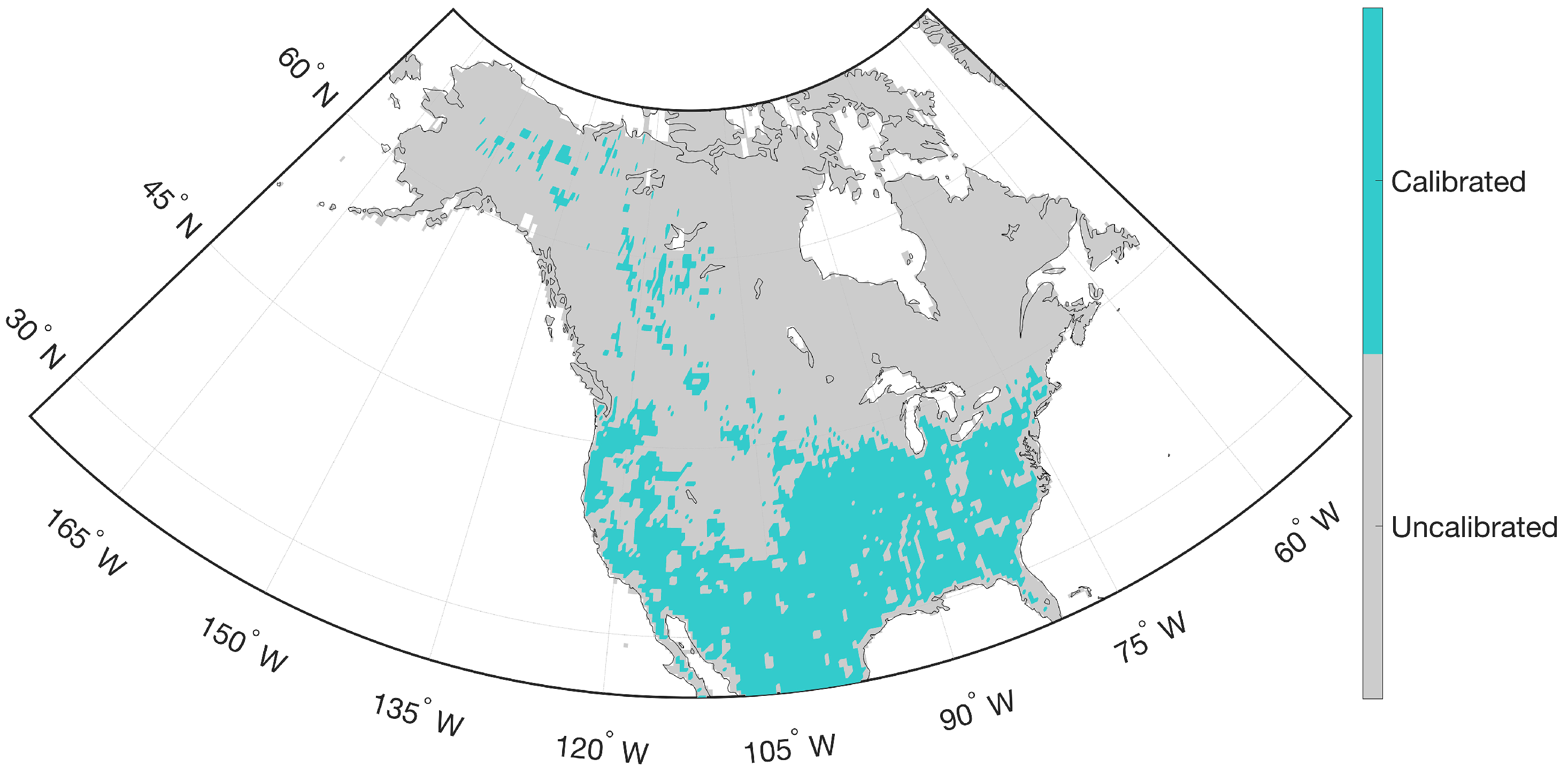
RTM-derived estimates were generated globally every 3 h on the 36-km Equal Area Scalable Earth (EASE) grid [52] in terrestrial areas with non-frozen soil conditions. RTM-derived estimates were locally calibrated using SMOS Level 1 version 504 observations to obtain climatologically unbiased estimates [44,53]. Prior to calibration, the available SMOS observations underwent extensive quality control. L-band microwave signals are often prone to contamination by RFI [54] that arises from a variety of transmitters used in communication applications, and were masked out accordingly. During the RTM calibration process using SMOS, further quality control was applied during frozen soil conditions when the model-based land surface temperature was less than K because the tau–omega model used here [44] is only applicable with non-frozen soils. Furthermore, SMOS observations collected near water bodies, during intense precipitation events (i.e., precipitation > 10 mm/h), or in the presence of snow cover (i.e., snow water equivalent kg/m2) were also excluded from calibration. Accordingly, the map of the calibrated and uncalibrated pixels over the North America study domain as illustrated in Figure 1 showed that most of the northern part of the study domain was not calibrated.
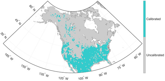
Figure 1.
Map of calibrated and uncalibrated areas across the North American study domain.
3.3. Aquarius Preprocessing
In order to collocate the GEOS RTM output with the corresponding Aquarius observations in space and time, the individual Aquarius overpasses were re-gridded (using a nearest neighbor approach) onto the 36-km Equal-Area Scalable Earth (EASE) grid, which is the same grid used for the processed SMOS observations as well as for the RTM simulations. For a given orbital track, the individual Aquarius observations that covered a given set of EASE grid cells were identified and then used to compute a mean value for that track on the corresponding EASE grid cells. If more than one Aquarius observation (over a collection period of a few seconds) fell within a single EASE grid cell, then the arithmetic average was applied to that entire cell. In addition, the value applied at a single cell center was also applied to the relevant neighboring cells (as a function of look angle) such that the approximate field-of-view for each of the three beams was correspondingly approximated on the relatively fine-scale 36-km EASE grid. The process was repeated for each of the three beams for every Aquarius overpass during the period 25 August 2011 through 7 June 2015, which represents the entire Aquarius measurement record. After preprocessing was complete, both the RTM-derived estimates (for all three beams) and the Aquarius observations (for all three beams) were matched in space and time for subsequent statistical analysis.
For quality assessment and quality control purposes, the time series of the RTM estimates and Aquarius observations were examined at each grid cell prior to statistical analysis. In order to focus on land-based estimates, 36-km EASE grid cells with a water fraction greater than 0.05 were excluded from the analysis because the observed Aquarius ’s did not represent the same physical processes as the RTM output (i.e., the RTM does not account for microwave emission from open water surfaces). In addition, grid cells with fewer than 40 pairs of Aquarius and RTM-derived observations collected over the course of the four-year study period were excluded from the analysis in order to yield statistically meaningful results.
3.4. Soil Classification and Hydraulic Properties
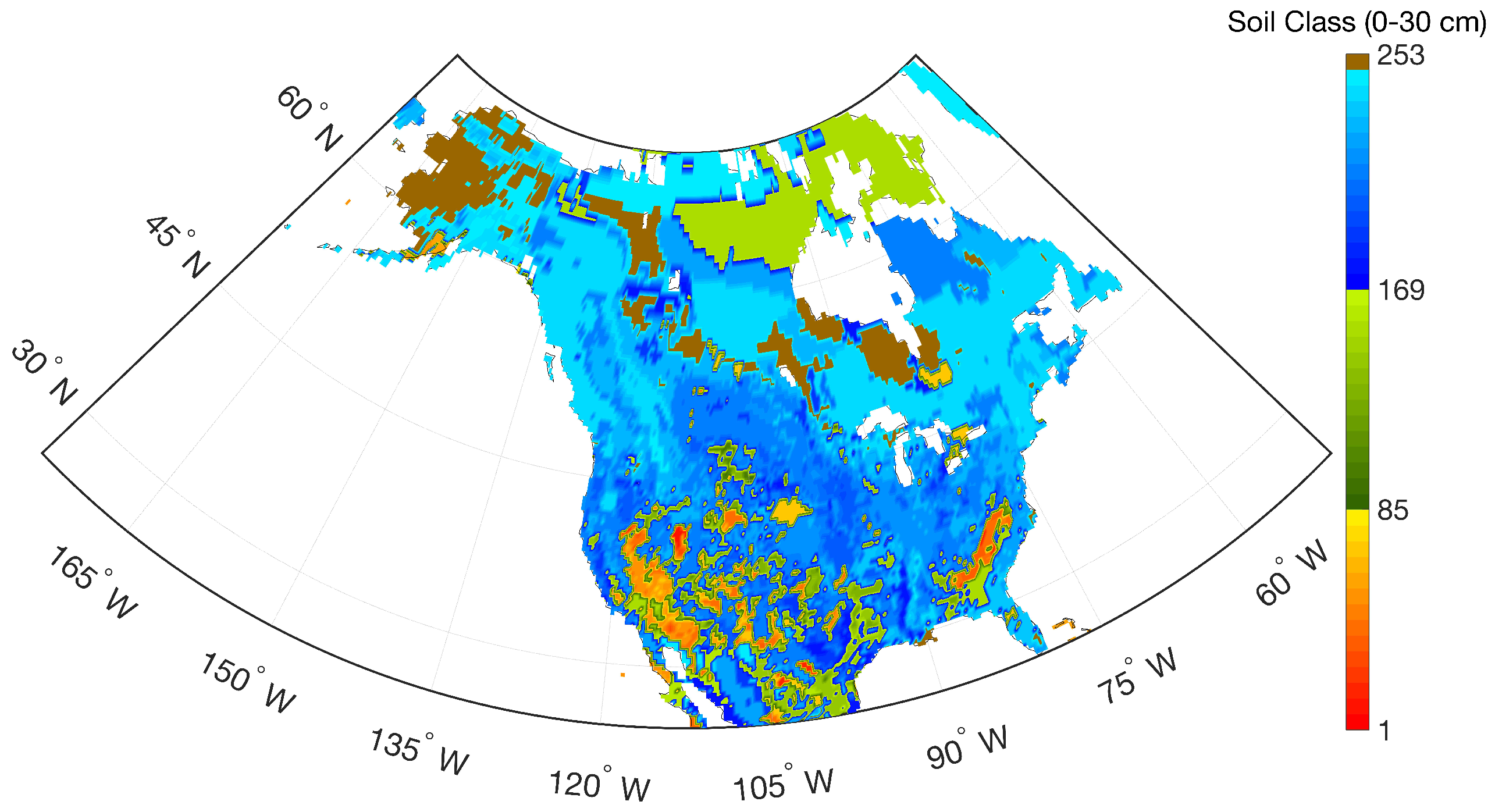
Soil classification used in this paper was based on the refined soil classification scheme introduced in De Lannoy et al. [53]. Data from the Harmonized World Soil Database and the State Soil Geographic Projects were used as a basis to derive the soil hydraulic properties and the soil organic content with a gridded resolution of . The classification of De Lannoy et al. [53] contains 253 soil classes, including 252 classes from three sets of low to moderate organic carbon categories, each with 84 different mineral classes defined from the refined soil texture triangle, plus one additional class (i.e., peat) with a very high organic content (Figure 2).

Figure 2.
Distribution of soil classes across North America for the top 30 cm of soil used in the radiative transfer model (RTM).
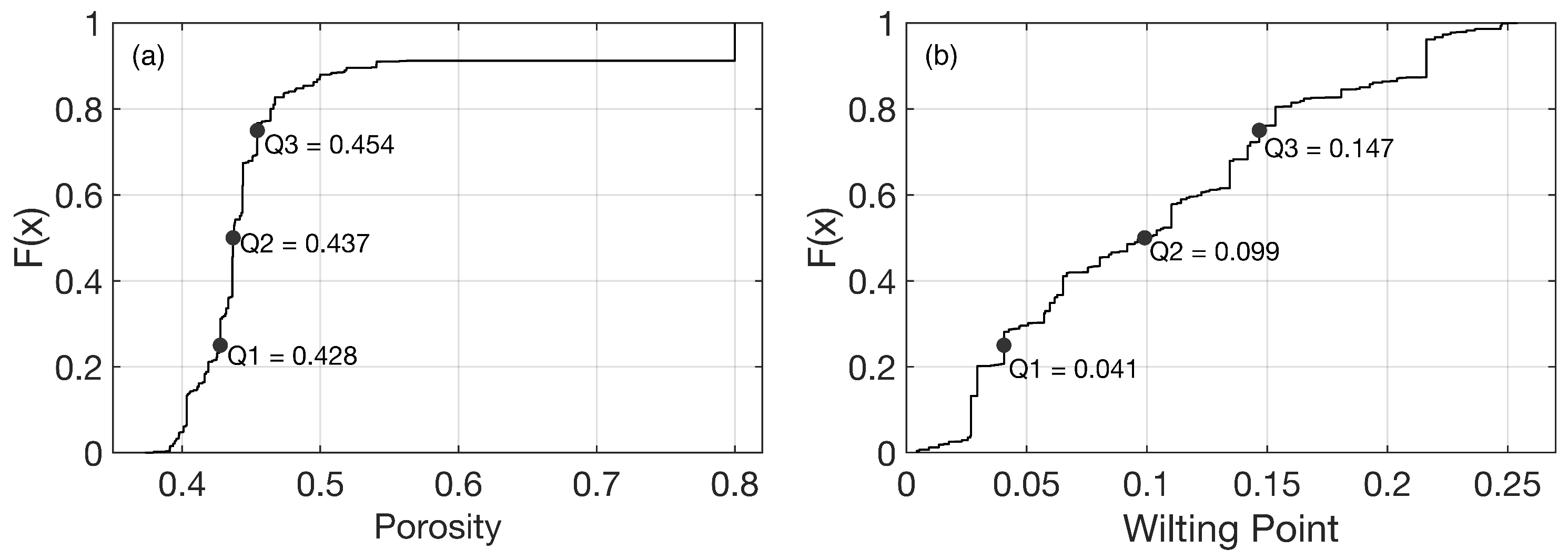
Based on the updated soil classification scheme, soil hydraulic parameters (SHPs) were determined through the pedotransfer functions suggested by Wosten et al. [55] using the percentage of clay, silt, and organic matter [53]. Among the SHPs, porosity and wilting point are selected for investigation in this paper as these parameters directly influence the dielectric constant and surface roughness variables that are used within the RTM. For the analysis, porosity and wilting point were divided into four different categories based on the quartile values drawn from the cumulative distribution function of each variable across the study domain (Figure 3). For example, Category I collects the value within the range of the zeroth to first quartile (0% to 25%) while Category IV collects the value from third to fourth quartile (75% to 100%).
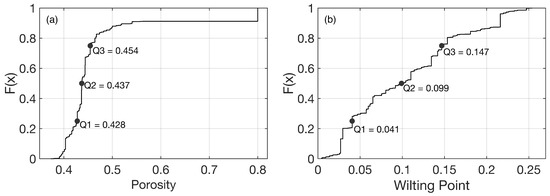
Figure 3.
Cumulative Distribution Function of (a) porosity and (b) wilting point within the study area. Q1 to Q3 represent the end points of the first to third quartile, respectively, and define the four categories used in Figures 8 and 9.
3.5. Vegetation and Irrigation Data
The vegetation classes utilized in this study are based on the Moderate Resolution Imaging Spectroradiometer (MODIS: 500 m MOD12Q1V004) International Geosphere–Biosphere Programme (IGBP) classification scheme [56]. For the analysis represented here, we mapped the 16 global IGBP classes into six dominant land cover classes across North America (i.e., evergreen and deciduous needleleaf forests merged into “needleleaf”; open and closed shrublands merged into “shrublands”) following the land cover schemes used for the Catchment model [57]. As the broadleaf evergreen forest accounts for less than 5% across the study area, it was excluded from the analysis. Accordingly, subsequent analyses presented in Section 4 as a function of vegetation type are discretized based on the five classes shown in Figure 4a and outlined in Table 1.
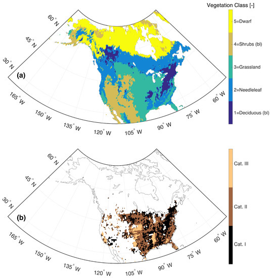
Figure 4.
Distribution of (a) lumped vegetation classes used in Section 4.3 and Table 1 and (b) irrigation categories based on the percentage of irrigated area relative to the total area based on the GMIA dataset [58].

Table 1.
Five lumped vegetation classes based on the International Geosphere–Biosphere Programme (IGBP) classification and used for the analysis in Section 4.3.
Furthermore, as cropland is lumped into the grassland category in the Catchment model, the Global Map of Irrigation Area (GMIA; Siebert et al. [58]) dataset is used to illustrate the percentage of area with actual irrigation relative to the total area in order to analyze the influence of irrigation over the grassland regions in the RTM-derived . As the GMIA dataset has a spatial resolution of 5 arc min by 5 arc min, it is resampled onto the 36 km EASE grid in order to coincide with the Catchment model. Further, the GMIA dataset was discretized into three sub-categories (i.e., 0–0.1%, 0.1–10%, 10–100%) (Figure 4b) based on the derived CDF (figure not shown).
3.6. Statistical Analysis
In this paper, bias and root mean square error (RMSE) are selected to evaluate the RTM-derived and are calculated as:
where n is the number of colocated (in space and time) brightness temperature observations and predictions, [K] is the brightness temperature predicted by the RTM, and [K] is the brightness temperature observed by Aquarius. In general, is a measure of systematic error that indicates the over- or under-prediction of the observation while RMSE accounts for both systematic and non-systematic (random) errors [59]. Additionally, unbiased root mean square error (ubRMSE) [60] was computed, which is the after first removing the bias.
4. Results and Discussion
4.1. Comparison between RTM, SMOS, and Aquarius Brightness Temperatures
Prior to analyzing the RTM-derived estimates, Aquarius observations were compared to both SMOS Level 1 version 504 and RTM-derived s colocated in space and time. This analysis is valuable, in that different behavior, as a function of incidence angle, influences the soil moisture retrieval as well as the structure of error covariance between the Catchment model and RTM-derived [37,61]. Figure 5 highlights the angular dependency of the spatiotemporal mean brightness temperatures across North America from co-located values among SMOS-, RTM-, and Aquarius-based ’s. The SMOS incidence angles that were closest to the corresponding Aquarius incidence angles were selected for comparison. In general, the mean at horizontal polarization decreases with increasing incidence angle for the RTM-derived and the observed estimates. Conversely, the mean at vertical polarization generally increases with increasing incidence angle for all estimates. However, from both SMOS and Aquarius showed little sensitivity (i.e., less than 1 K) from to at vertical polarization, in contrast to the corresponding RTM-derived .
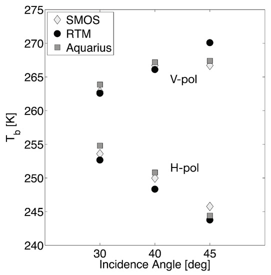
Figure 5.
Spatio-temporally averaged across the study period (from 25 August 2011 to 7 June 2015) over North America as a function of incidence angle from Soil Moisture Ocean Salinity (SMOS), radiative transfer model (RTM), and Aquarius.
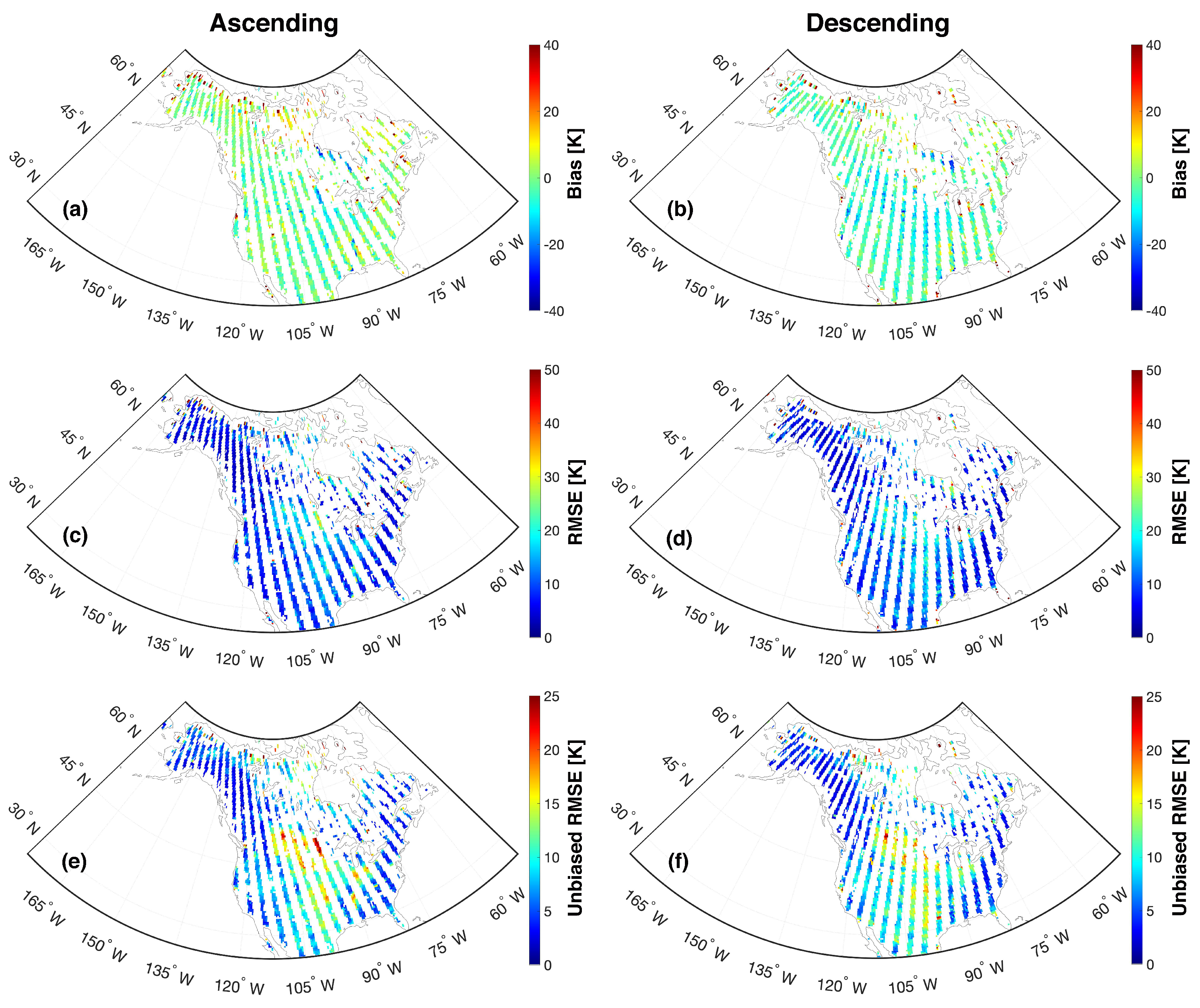
Figure 6 highlights the statistical skill of the RTM-derived estimates for beam #1 at horizontal polarization (relative to Aquarius) using ascending and descending overpasses across North America. The bias map in Figure 6a,b shows that computed bias (represented to three significant digits) ranged from −8.13 K to 8.58 K (ascending overpasses) and −11.7 K to 4.55 K (descending overpasses) with domain-averaged biases of 0.79 K and −2.79 K for ascending and descending overpasses, separately. The majority of observations in northern Canada were excluded during quality control based on an insufficient number of available observations during non-frozen soil conditions. This screening was needed because the RTM only predicts during non-frozen soil conditions (see Section 2). The same behavior was witnessed for both horizontal and vertical polarizations but only results for horizontal polarization are presented here. For beam #2 (figure not shown) the bias ranges from −12.8 K to 8.85 K while for beam #3 (figure not shown), the bias ranges from −14.1 K to 8.40 K collectively for the ascending and descending overpasses. The results for vertical polarization bias are comparable to that of horizontal polarization with values ranging predominantly from −9.14 K to 8.96 K (figure not shown). The regions in the northern part of Canada near Lake Winnipeg and Hudson Bay have a relatively high magnitude of negative bias (i.e., exceeding −13.3 K) across the different beams and polarization. Locations immediately next to water bodies near Lake Winnipeg, Hudson Bay, Great Lakes, and the Great Salt Lake have anomalously large, positive biases (approximately 40 K). In addition, some large areas in and around the boreal forest regions in northern Canada show higher bias (18.6 K and 12.7 K for ascending and descending overpasses, respectively), which is also likely due to the presence of a significant number of sub-grid scale lakes. These phenomena are further exacerbated by the resampling of the Aquarius onto a relatively finer scale grid. That is, Aquarius was rescaled (a.k.a. oversampled) onto the 36-km EASE grid in order to facilitate the comparison with RTM-derived . However, when the footprint of the Aquarius includes open water bodies that extend beyond a particular 36-km EASE grid cell, the regridded neighboring pixels will still contain information partially contaminated by the nearby open water bodies. Additionally, the lack of a module for open water in the current RTM also resulted in some strongly biased simulation result.
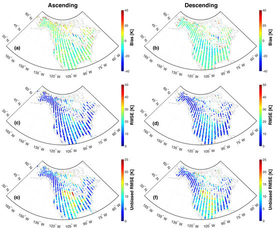
Figure 6.
Statistical maps of bias (a,b), root mean square error (RMSE) (c,d), and unbiased RMSE (e,f) between Aquarius and RTM-derived during the study period (25 August 2011 to 7 June 2015) over North America for beam #1 at H-polarization. The Left and right columns represent the ascending and descending overpasses, respectively.
Similar patterns are seen in the RMSE (Figure 6c,d) and ubRMSE (Figure 6e,f) statistics for ascending and descending overpasses for beam #1 at horizontal polarization. Nearly identical patterns are witnessed for the other beam and polarization combinations (not shown). The computed RMSEs are within the range of 4.13 K to 18.9 K for both ascending and descending overpasses across the study domain for all three beams at horizontal polarization. However, vertical polarization RMSE results are, in general, smaller than their horizontal polarization counterparts with RMSE values generally ranging from 3.99 K to 16.4 K, 4.14 K to 15.2 K, and 3.83 K to 14.8 K for beams #1, #2, and #3, respectively (not shown). Large RMSE values are found in the northern part of Canada and near large water bodies associated with correspondingly large bias values (see Figure 6a,b) Unbiased RMSE results are shown in Figure 6e,f for beam #1 at horizontal polarization, and typically range from 0 K to 14.2 K, except in the central United States and Canada, where values typically range from 12.0 K to 17.7 K for both ascending and descending overpasses. Similar ranges of unbiased RMSE were found for beams #2 and #3 at horizontal polarization. The ubRMSE values are slightly smaller at vertical polarization and typically range between 10.1 K to 15.2 K in the Central United States and between 1.39 K to 5.43 K everywhere else.
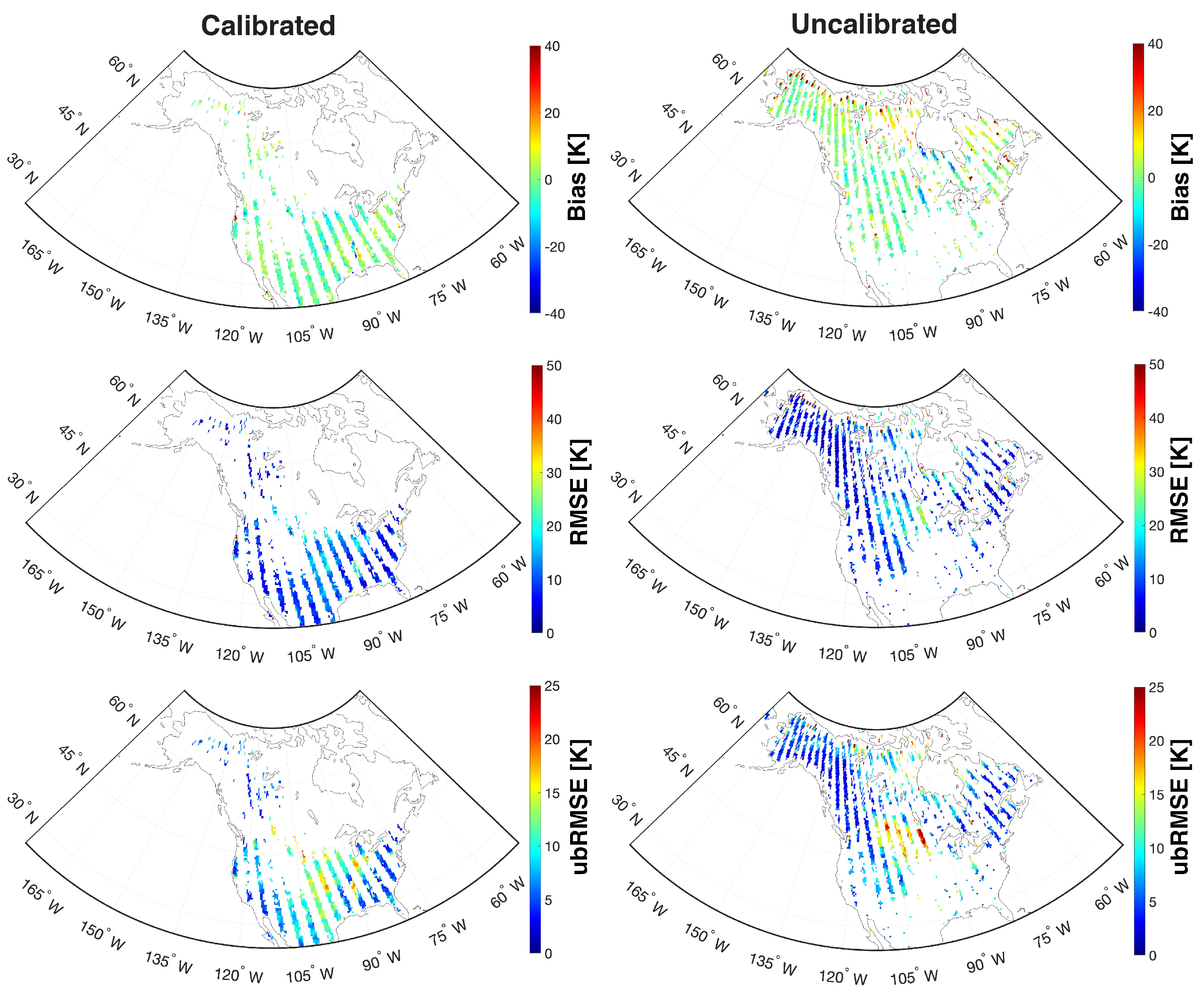
Statistical performance of calibrated and uncalibrated pixels with ascending overpasses are shown in Figure 7. Note that the majority of the northern portion of the study domain was not selected for calibration as discussed in Section 3.2. The overall results confirmed that calibrated pixels showed better performance than uncalibrated pixels. Computed bias ranged from −7.03 K to 4.00 K (calibrated pixels) and −7.48 K to 8.33 K (uncalibrated pixels) with domain-averaged bias of 0.79 K and 2.17 K for calibrated and uncalibrated pixels, respectively. The descending overpasses also showed similar behavior as the ascending overpasses with the calculated bias ranging from −10.1 K to 0.92 K and −9.73 to 3.43 K for calibrated and uncalibrated pixels, respectively. Similar behavior was observed for RMSE and ubRMSE in that calibrated pixels fall within the range of 3.31 K to 18.2 K (RMSE) and 2.45 K to 14.3 K (ubRMSE) while uncalibrated pixels yielded a RMSE range from 3.77 K to 20.1 K and ubRMSE range from 2.86 K to 15.1 K across the combination of ascending and descending overpasses. As most of the regions near the water bodies and the northern boreal forest were excluded from the calibration (Figure 1), they exhibited a relatively high magnitude of bias, RMSE, and ubRMSE as compared to other regions. Focusing on the middle part of the study area where there is a high percentage of irrigation (Figure 4b), both calibrated and uncalibrated pixels showed relatively high bias, RMSE, and ubRMSE (Figure 7). Detailed discussion about RTM performance over irrigated areas is further discussed in Section 4.3.
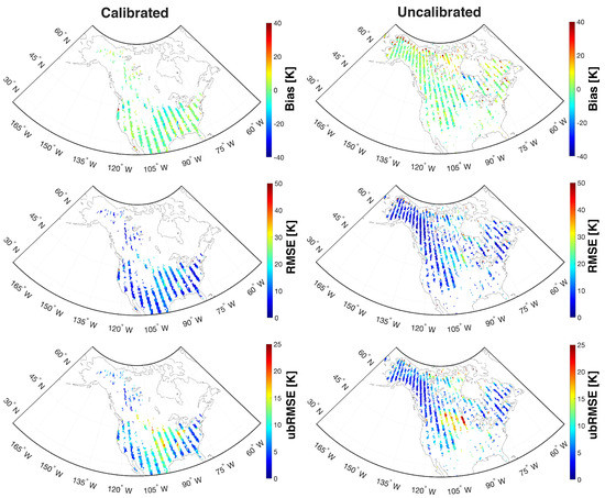
Figure 7.
Statistical maps of bias (top row), RMSE (middle row), and unbiased RMSE (bottom row) between Aquarius and RTM-derived during the study period (25 August 2011 to 7 June 2015) over North America for beam #1 at H-polarization. The Left and right columns represent the calibrated and uncalibrated pixels, respectively. Note that the majority of the northern portions of the study domain were excluded from the calibration exercise due to significant periods of time with frozen surface soil conditions and/or the presence of significant amounts of sub-grid scale lakes (Section 3.2).
4.2. Performance as a Function of Soil Hydraulic Parameters
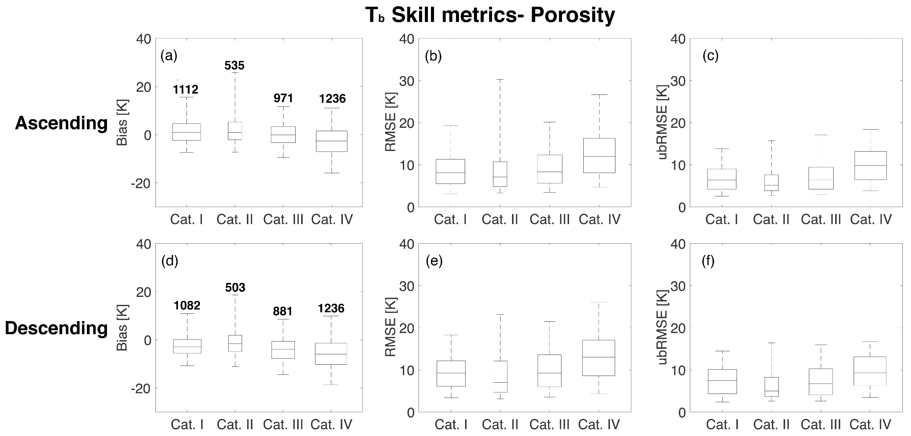
Figure 8 and Figure 9 show the statistical results of the comparison of RTM and Aquarius as a function of porosity and wilting point, respectively. The whisker ranges from the 5th to 95th percentiles of the computed statistics whereas the boxplot highlights the 75th, 50th, and 25th percentiles. Figure 8 suggests that the highest porosity (Category IV) corresponds to the poorest agreement between the RTM-derived estimates and the Aquarius observations for both ascending (−2.62 K) and descending (−5.94 K) overpasses. The median bias (i.e., 50th percentile of the boxes shown in the leftmost column of the subplots) is lowest in Category III for ascending overpasses with a value of −0.05 K and Category II for descending overpasses with a value of −1.58 K. RMSE and ubRMSE plots presented in the second and third columns of Figure 8 also revealed that the highest porosity category showed the highest median values of 11.9 K (RMSE) and 9.83 K (ubRMSE) for ascending overpasses and 13.0 K (RMSE) and 9.31 K (ubRMSE) for descending overpasses. Similar to the behavior of porosity, a higher wilting point, in general, corresponds to a weaker agreement between the RTM-derived estimates and the Aquarius observations (Figure 9). Median bias for the four wilting point categories are 1.41 K, 0.50 K, −0.40 K, and −2.67 K for ascending overpasses and −1.98 K, −2.89 K, −4.29 K, and −5.80 K for descending overpasses, respectively. RMSE and ubRMSE for the different wilting point categories also suggest more RTM uncertainty in the highest wilting point category (Category IV) with values of 11.7 K (RMSE) and 9.32 K (ubRMSE) for ascending overpasses and 12.7 K (RMSE) and 9.15 K (ubRMSE) for descending overpasses, respectively.

Figure 8.
Statistical comparison for different porosity categories based on the CDF (Figure 3a) for beam #1 at H-polarization. The different rows show the results for ascending and descending overpasses. The different columns represent the results of bias, RMSE, and unbiased RMSE. The upper and lower whiskers represent 95th and 5th percentiles, respectively, whereas the boxes show the median line along with 75th and 25th percentiles. The number over the boxes in the first column indicates the number of samples for each category.
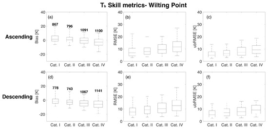
Figure 9.
Statistical comparison for different wilting point categories based on the CDF (Figure 3b) for beam #1 at H-polarization. The different rows show results for ascending and descending overpasses. The different columns represent the results of bias, RMSE, and unbiased RMSE. The upper and lower whiskers represent 95th and 5th percentiles, respectively, whereas the boxes show the median line along with 75th and 25th percentiles. The number over the boxes in the first column indicates the number of samples for each category.
High values of uncertainty for soils with large porosity or large wilting point can be explained through their influence on the surface roughness and dielectric constant. Soils with higher porosity or wilting point tend to have a higher fraction of clay [48]. As clay has a large surface-to-volume ratio (relative to other soil types), it has an affinity for binding a greater percentage of water molecules, which causes a variation in the dielectric constant [18]. Additionally, an increase in wilting point or porosity will influence the calculation of surface roughness in the RTM when the soil moisture falls between the transition point and porosity [44]. Another reason is related to the lack of SMOS observations for use during calibration over regions parameterized as peat, which features high porosity values (approximately 0.8). Because peatlands are typically also water-rich, the screening of SMOS data for open water fractions less than 0.05 yielded a limited number of observations in these areas.
4.3. Performance as a Function of Vegetation Type
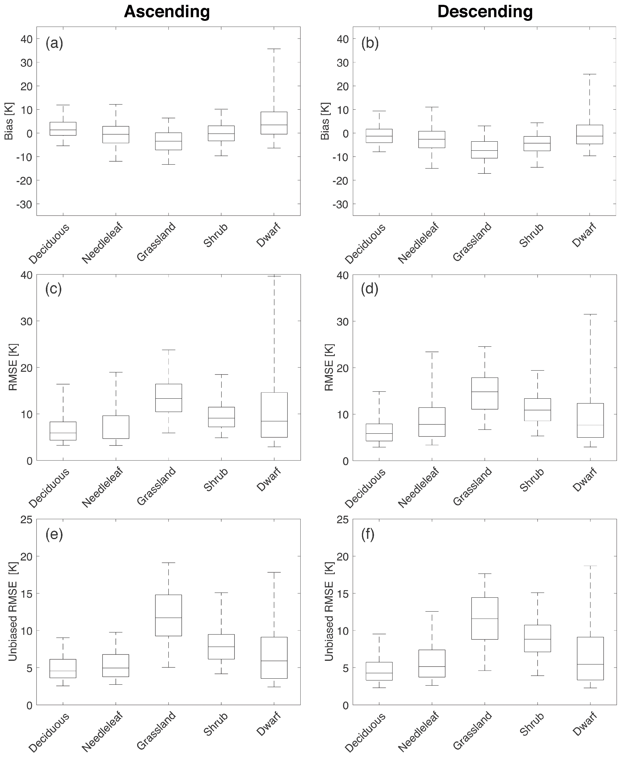
In a similar manner as conducted for soil hydraulic parameters, a statistical evaluation of predicted performance was conducted as a function of vegetation type separately over ascending and descending overpasses. Statistical comparisons for horizontal polarization are shown in Figure 10. Broadleaf deciduous and needleleaf forest suggest better agreement (i.e., lower median bias, RMSE, and ubRMSE) between the RTM and the observations relative to other vegetation classes. Median bias, RMSE, and ubRMSE ranged from −2.63 K to 1.37 K, 5.84 K to 7.82 K, and 4.29 K to 5.16 K, respectively, for broadleaf deciduous and needleleaf forest classes for beam #1 at H-polarization. In terms of the range between the 5th and 95th percentile values of bias and RMSE, the grassland and shrub vegetation types showed a narrower range than dwarf vegetation. However, the RMSE and ubRMSE plots showed poor performance in estimation in grasslands (median RMSE between 6.40 K to 14.8 K and median ubRMSE between 6.80 K to 11.7 K) across the different overpasses at both polarizations.
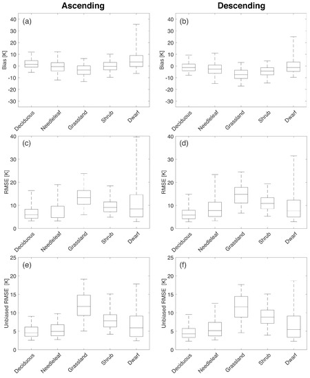
Figure 10.
Statistical comparisons over the dominant vegetation classes (Table 1 and Figure 4a) for beam #1 at H-polarization. The different rows show the results of bias, RMSE, and unbiased RMSE. The different columns show results for ascending and descending overpasses. The upper and lower whiskers represent 95th and 5th percentiles, respectively, whereas the boxes show the median line along with 75th and 25th percentiles.
De Lannoy et al. [44] also revealed similar behavior in that estimates from the RTM exhibited low uncertainties over dense vegetation while large uncertainties were observed over regions with grassland vegetation type. Poor performance in grassland regions might result from poorly parameterized agricultural croplands, which is included in the category of grassland (Table 1). Statistical comparison of Aquarius and RTM-derived in accordance with the different percentages of irrigated areas within a pixel revealed that pixels with more than 10% of the irrigated area showed the most negative bias for ascending and descending overpasses (Table 2). Moreover, according to Figure 4, irrigation-dominated regions including parts of Nebraska, the Lower Mississippi River Basin, and the California Central Valley [62] are classified as grassland even though they are intensively irrigated croplands. De Lannoy and Reichle [37] and Rains et al. [63] showed the potential capability of SMOS observations to reflect irrigation. This result suggests that predicted will likely be less accurate due to a lack of an explicit irrigation scheme in the land surface model (and hence not considered in the RTM) [64].

Table 2.
Statistical comparison of RTM-derived for beam #1 horizontal polarization as a function of the percentage of pixel area with irrigation (I) as estimated by the GMIA dataset. Units for bias, RMSE, and ubRMSE are K.
Irrigation, in general, makes soil wetter and lowers the physical temperature via adding relatively cool water to warm soil, in conjunction with evaporative cooling, which leads to a lower . RTM-derived accounts for microwave emission from the soil surface as well as the overlying vegetation (Equation (1)). Since the Catchment model lacks an explicit irrigation module and generally underestimates soil moisture in irrigated regions, the effective microwave roughness height (Equation (5)) and surface reflectivity (Equation (4)) tend to be overestimated, which, in turn, results in an overestimation of the microwave emission from the soil surface (or a warm bias in ). At the same time, however, the lack of an irrigation scheme along with the misclassification of cropland vegetation as grassland vegetation, also leads to errors in the modeled vegetation properties. For example, vegetation-related RTM parameters (e.g., vegetation structure parameter, vegetation attenuation, and vegetation water content) tend to be underestimated, which in turn, results in an underestimation of microwave emission from the vegetation (or a cold bias in ). Additionally, the monthly-varying, climatological LAI estimates utilized in the Catchment model do not reflect inter-annual crop rotations. The combination of these different factors can result in the underestimation of RTM-derived estimates when compared against Aquarius observations.
5. Conclusions
L-band estimates from an RTM calibrated using SMOS observations were evaluated against Aquarius observations in order to examine the applicability of multi-year SMOS , which exhibited similar climatology as Aquarius [32,33], in order to simulate Aquarius . This experimental setting allows for an independent evaluation of RTM-derived against the Aquarius observations. The evaluation process was conducted across a range of soil hydraulic parameters and vegetation types for the period from 25 August 2011 to 7 June 2015. Analyses were performed at all three incidence angles (, , and , a.k.a., beams #1, #2, and #3) from Aquarius at both horizontal and vertical polarizations, and for ascending and descending overpasses.
Bias, RMSE, and ubRMSE were calculated to investigate the degree of agreement between the RTM and Aquarius . Areas near to, or with, dynamic ponding or static lakes exhibited relatively large uncertainties due to the oversampling of Aquarius as well as lack of an open water module in the current RTM. Statistics computed over different soil hydraulic parameters (e.g., porosity and wilting point) revealed that higher porosity and higher wilting point corresponded to poorer performance due to the variation in surface roughness and dielectric constant.
Among the vegetation classes, broadleaf deciduous and needleleaf forest yielded the best statistics in terms of bias, RMSE, and ubRMSE. The RTM exhibited better performance in regions of dwarf vegetation as compared to the shrub land and grassland vegetation types. The RTM exhibited the lowest accuracy in the grassland class among the five different vegetation classes, which is largely attributed to regions of agricultural irrigation and a lack of local irrigation schemes as well as a lack of inter-annual crop rotations in the land surface model that serves as the input to the RTM.
In summary, it was shown that SMOS observations serve as an effective calibration dataset for the RTM-derived estimates of Aquarius . RTM-derived as evaluated in this study does a reasonable job reproducing observations from Aquarius over different soil hydraulic properties and vegetation types across North America. Better agreement between the RTM-derived estimates and the Aquarius-derived observations was witnessed at lower porosity and wilting point values. The RTM-derived yielded reasonable statistics for most vegetation types while further consideration of cropland (which is classified as grasslands in this study) could improve the accuracy of the RTM. These findings can be leveraged for the eventual inclusion of Aquarius L-band in a follow-on study using a data assimilation framework for the purpose of improving model-derived estimates of soil moisture. For example, as most of the northern portions of the study domain were not calibrated due to the presence of abundant sub-grid scale lakes, relaxing the constraints of SMOS with regards to the distance to open water bodies could assure more SMOS observations for use during calibration. Furthermore, an update of the current RTM by including a module for open water should also be considered. In terms of error characterization, larger observation errors need to be assigned for grassland areas as well as for regions with high porosity soil and high wilting points.
Author Contributions
J.P. and B.A.F. designed and conducted the experiments and analyzed results with help of B.A.F., R.H.R., G.D.L. and S.B.T.; R.H.R. and G.D.L. prepared initial setup of the Catchment land surface model and RTM simulation; J.P. and B.A.F. wrote the paper, and all other authors contributed to improving the paper. All authors have read and agreed to the published version of the manuscript.
Funding
R.H.R. was supported by the NASA SMAP mission and the SMAP Science Team. G.D.L. was supported by the Research Foundation Flanders (FWO-1512817N) and KU Leuven C1 internal fund C14/16/045.
Acknowledgments
Aquarius data were obtained as a Level-2 (single orbit) product produced at the NASA Jet Propulsion Laboratory and available at http://podaac.jpl.nasa.gov/aquarius. The GEOS source code is available under the NASA Open-Source Agreement at http://opensource.gsfc.nasa.gov/projects/GEOS-5. Computational resources were provided by the NASA High-End Computing program through the NASA Center for Climate Simulation. Additional high-performance computing support was provided by the Division of Information Technology (DIT) at the University of Maryland.
Conflicts of Interest
The authors declare no conflict of interest.
References
- Qiu, J.; Mo, X.; Liu, S.; Lin, Z.; Yang, L.; Song, X.; Zhang, G.; Naeimi, V.; Wagner, W. Intercomparison of microwave remote-sensing soil moisture data sets based on distributed eco-hydrological model simulation and in situ measurements over the North China Plain. Int. J. Remote Sens. 2013, 34, 6587–6610. [Google Scholar] [CrossRef]
- Su, C.H.; Ryu, D.; Young, R.I.; Western, A.W.; Wagner, W. Inter-comparison of microwave satellite soil moisture retrievals over the Murrumbidgee Basin, southeast Australia. Remote Sens. Environ. 2013, 134, 1–11. [Google Scholar] [CrossRef]
- Wang, T.; Franz, T.E.; Li, R.; You, J.; Shulski, M.D.; Ray, C. Evaluating climate and soil effects on regional soil moisture spatial variability using EOFs. Water Resour. Res. 2017, 53, 242–253. [Google Scholar] [CrossRef]
- Guillod, B.P.; Orlowsky, B.; Miralles, D.G.; Teuling, A.J.; Seneviratne, S.I. Reconciling spatial and temporal soil moisture effects on afternoon rainfall. Nat. Commun. 2015, 6, 6443. [Google Scholar] [CrossRef] [PubMed]
- Koster, R.D.; Dirmeyer, P.A.; Guo, Z.; Bonan, G.; Chan, E.; Cox, P.; Gordon, C.T.; Kanae, S.; Kowalczyk, E.; Lawrence, D.; et al. Regions of strong coupling between soil moisture and precipitation. Science 2004, 305, 1138–1140. [Google Scholar] [CrossRef] [PubMed]
- Brubaker, K.L.; Entekhabi, D. An Analytic Approach to Modeling Land-Atmosphere Interaction: 1. Construct and Equilibrium Behavior. Water Resour. Res. 1995, 31, 619–632. [Google Scholar] [CrossRef]
- Corradini, C. Soil moisture in the development of hydrological processes and its determination at different spatial scales. J. Hydrol. 2014, 516, 1–5. [Google Scholar] [CrossRef]
- Delworth, T.; Manabe, S. The influence of soil wetness on near-surface atmospheric variability. J. Clim. 1989, 2, 1447–1462. [Google Scholar] [CrossRef]
- Entekhabi, D.; Rodriguez-Iturbe, I.; Castelli, F. Mutual interaction of soil moisture state and atmospheric processes. J. Hydrol. 1996, 184, 3–17. [Google Scholar] [CrossRef]
- Harrison, K.W.; Kumar, S.V.; Peters-Lidard, C.D.; Santanello, J.A. Quantifying the change in soil moisture modeling uncertainty from remote sensing observations using Bayesian inference techniques. Water Resour. Res. 2012, 48, W11514. [Google Scholar] [CrossRef]
- Moradkhani, H. Hydrologic remote sensing and land surface data assimilation. Sensors 2008, 8, 2986–3004. [Google Scholar] [CrossRef] [PubMed]
- Reichle, R.H.; McLaughlin, D.B.; Entekhabi, D. Hydrologic Data Assimilation with the Ensemble Kalman Filter. Mon. Weather Rev. 2002, 130, 103–114. [Google Scholar] [CrossRef]
- Xia, Y.; Sheffield, J.; Ek, M.B.; Dong, J.; Chaney, N.; Wei, H.; Meng, J.; Wood, E.F. Evaluation of Multi-Model Simulated Soil Moisture in NLDAS-2. J. Hydrol. 2014, 512, 107–125. [Google Scholar] [CrossRef]
- Koster, R.D.; Suarez, M.J.; Higgins, R.W.; Van den Dool, H.M. Observational evidence that soil moisture variations affect precipitation. Geophys. Res. Lett. 2003, 30, 1241. [Google Scholar] [CrossRef]
- Seneviratne, S.I.; Corti, T.; Davin, E.L.; Hirschi, M.; Jaeger, E.B.; Lehner, I.; Orlowsky, B.; Teuling, A.J. Investigating soil moisture—Climate interactions in a changing climate: A review. Earth Sci. Rev. 2010, 99, 125–161. [Google Scholar] [CrossRef]
- Berkhuijsen, E.M. A consistent scheme of definitions of polarisation brightness temperature and brightness temperature. Astron. Astrophys. 1975, 40, 311–316. [Google Scholar]
- Matzler, C. On the determination of surface emissivity from satellite observations. IEEE Geosci. Remote Sens. Lett. 2005, 2, 160–163. [Google Scholar] [CrossRef]
- Njoku, E.G.; Entekhabi, D. Passive microwave remote sensing of soil moisture. J. Hydrol. 1996, 184, 101–129. [Google Scholar] [CrossRef]
- Schmugge, T.J. Remote sensing of soil moisture: Recent advances. IEEE Trans. Geosci. Remote Sens. 1983, 21, 336–344. [Google Scholar] [CrossRef]
- Schmugge, T.; Jackson, T.J. Mapping surface soil moisture with microwave radiometers. Meteorol. Atmos. Phys. 1994, 54, 213–223. [Google Scholar] [CrossRef]
- Schmugge, T.J.; Kustas, W.P.; Ritchie, J.C.; Jackson, T.J.; Rango, A. Remote sensing in hydrology. Adv. Water Resour. 2002, 25, 1367–1385. [Google Scholar] [CrossRef]
- Kerr, Y.H.; Waldteufel, P.; Wigneron, J.P.; Martinuzzi, J.; Font, J.; Berger, M. Soil moisture retrieval from space: The Soil Moisture and Ocean Salinity (SMOS) mission. IEEE Trans. Geosci. Remote Sens. 2001, 39, 1729–1735. [Google Scholar] [CrossRef]
- Kerr, Y.H.; Wigneron, J.P.; Delwart, S.; Cabot, F.; Boutin, J.; Escorihuela, M.J.; Font, J.; Reul, N.; Gruhier, C.; Juglea, S.E.; et al. The SMOS Mission: New Tool for Monitoring Key Elements of the Global Water Cycle. Proc. IEEE 2010, 98, 666–687. [Google Scholar] [CrossRef]
- Leroux, D.J.; Kerr, Y.H.; Wood, E.F.; Sahoo, A.K.; Bindlish, R.; Jackson, T.J. An Approach to Constructing a Homogeneous Time Series of Soil Moisture Using SMOS. IEEE Trans. Geosci. Remote Sens. 2014, 52, 393–405. [Google Scholar] [CrossRef]
- Al Bitar, A.; Leroux, D.; Kerr, Y.H.; Merlin, O.; Richaume, P.; Sahoo, A.; Wood, E.F. Evaluation of SMOS soil moisture products over Continental U.S. using the SCAN/SNOTEL network. IEEE Trans. Geosci. Remote Sens. 2012, 50, 1572–1586. [Google Scholar] [CrossRef]
- Al-Yaari, A.; Wigneron, J.P.; Dorigo, W.; Colliander, A.; Pellarin, T.; Hahn, S.; Mialon, A.; Richaume, P.; Fernandez-Moran, R.; Fan, L.; et al. Assessment and inter-comparison of recently developed/reprocessed microwave satellite soil moisture products using ISMN ground-based measurements. Remote Sens. Environ. 2019, 224, 289–303. [Google Scholar] [CrossRef]
- Jackson, T.J.; Bindlish, R.; Cosh, M.H.; Zhao, T.; Starks, P.J.; Bosch, D.D.; Seyfried, M.; Moran, M.S.; Goodrich, D.C.; Kerr, Y.H.; et al. Validation of Soil Moisture and Ocean Salinity (SMOS) Soil Moisture Over Watershed Networks in the U.S. IEEE Trans. Geosci. Remote Sens. 2012, 50, 1530–1543. [Google Scholar] [CrossRef]
- Pan, M.; Sahoo, A.K.; Wood, E.F.; Al Bitar, A.; Leroux, D.; Kerr, Y.H. An initial assessment of SMOS derived soil moisture over the continental United States. IEEE J. Sel. Top. Appl. Earth Obs. Remote Sens. 2012, 5, 1448–1457. [Google Scholar] [CrossRef]
- Schaefer, G.L.; Cosh, M.H.; Jackson, T.J. The USDA Natural Resources Conservation Service Soil Climate Analysis Network (SCAN). J. Atmos. Ocean. Technol. 2007, 24, 2073–2077. [Google Scholar] [CrossRef]
- Entekhabi, D.; Njoku, E.G.; O’Neill, P.E.; Kellogg, K.H.; Crow, W.T.; Edelstein, W.N.; Entin, J.K.; Goodman, S.D.; Jackson, T.J.; Johnson, J.; et al. The Soil Moisture Active Passive (SMAP) Mission. Proc. IEEE 2010, 98, 704–716. [Google Scholar] [CrossRef]
- Le Vine, D.M.; Lagerloef, G.S.E.; Colomb, F.R.; Yueh, S.H.; Member, S.; Pellerano, F.A. Aquarius: An Instrument to Monitor Sea Surface Salinity From Space. IEEE Trans. Geosci. Remote Sens. 2007, 45, 2040–2050. [Google Scholar] [CrossRef]
- Pablos, M.; Piles, M.; González-Gambau, V.; Vall-llossera, M.; Camps, A. Inter-comparison of SMOS and aquarius brightness temperatures at L-band over selected targets. In Proceedings of the 2013 IEEE International Geoscience and Remote Sensing Symposium—IGARSS, Melbourne, Australia, 21–26 July 2013; pp. 386–389. [Google Scholar] [CrossRef]
- Piepmeier, J.; Brown, S.; Gales, J.; Hong, L.; Lagerloef, G.; Le Vine, D.; de Matthaeis, P.; Meissner, T.; Bindlish, R.; Jackson, T.; et al. Aquarius Radiometer Post-Launch Calibration for Product Version 2; Technical Report; National Aeronautics and Space Administration: Washington, DC, USA, 2013.
- Bindlish, R.; Jackson, T.; Cosh, M.; Zhao, T.; O’Neill, P. Global Soil Moisture From the Aquarius/SAC-D Satellite: Description and Initial Assessment. IEEE Geosci. Remote Sens. Lett. 2015, 12, 923–927. [Google Scholar] [CrossRef]
- Carrera, M.L.; Bilodeau, B.; Bélair, S.; Abrahamowicz, M.; Russell, A.; Wang, X. Assimilation of Passive L-band Microwave Brightness Temperatures in the Canadian Land Data Assimilation System: Impacts on Short-Range Warm Season Numerical Weather Prediction. J. Hydrometeorol. 2019, 20, 1053–1079. [Google Scholar] [CrossRef]
- Crow, W.T.; Wood, E.F. The assimilation of remotely sensed soil brightness temperature imagery into a land surface model using Ensemble Kalman filtering: A case study based on ESTAR measurements during SGP97. Adv. Water Resour. 2003, 26, 137–149. [Google Scholar] [CrossRef]
- De Lannoy, G.J.M.; Reichle, R.H. Assimilation of SMOS brightness temperatures or soil moisture retrievals into a land surface model. Hydrol. Earth Syst. Sci. 2016, 20, 4895–4911. [Google Scholar] [CrossRef]
- Lievens, H.; Reichle, R.H.; Liu, Q.; De Lannoy, G.J.M.; Dunbar, R.S.; Kim, S.B.; Das, N.N.; Cosh, M.; Walker, J.P.; Wagner, W. Joint Sentinel-1 and SMAP data assimilation to improve soil moisture estimates. Geophys. Res. Lett. 2017, 44, 6145–6153. [Google Scholar] [CrossRef]
- Reichle, R.H.; De Lannoy, G.J.M.; Liu, Q.; Ardizzone, J.V.; Colliander, A.; Conaty, A.; Crow, W.; Jackson, T.J.; Jones, L.A.; Kimball, J.S.; et al. Assessment of the SMAP Level-4 Surface and Root-Zone Soil Moisture Product Using In Situ Measurements. J. Hydrometeorol. 2017, 18, 2621–2645. [Google Scholar] [CrossRef]
- Reichle, R.H.; De Lannoy, G.J.M.; Liu, Q.; Koster, R.D.; Kimball, J.S.; Crow, W.T.; Ardizzone, J.V.; Chakraborty, P.; Collins, D.W.; Conaty, A.L.; et al. Global Assessment of the SMAP Level-4 Surface and Root-Zone Soil Moisture Product Using Assimilation Diagnostics. J. Hydrometeorol. 2017, 18, 3217–3237. [Google Scholar] [CrossRef]
- Reichle, R.H.; Liu, Q.; Koster, R.D.; Crow, W.T.; De Lannoy, G.J.; Kimball, J.S.; Ardizzone, J.V.; Bosch, D.; Colliander, A.; Cosh, M.; et al. Version 4 of the SMAP Level-4 Soil Moisture Algorithm and Data Product. J. Adv. Model. Earth Syst. 2019, 11. [Google Scholar] [CrossRef]
- Sabater, J.M.; Lawrence, H.; Albergel, C.; Rosnay, P.; Isaksen, L.; Mecklenburg, S.; Kerr, Y.; Drusch, M. Assimilation of SMOS brightness temperatures in the ECMWF Integrated Forecasting System. Q. J. R. Meteorol. Soc. 2019, 145, 2524–2548. [Google Scholar] [CrossRef]
- Jia, B.; Tian, X.; Xie, Z.; Liu, J.; Shi, C. Assimilation of microwave brightness temperature in a land data assimilation system with multi-observation operators. J. Geophys. Res. Atmos. 2013, 118, 3792–3985. [Google Scholar] [CrossRef]
- De Lannoy, G.J.M.; Reichle, R.H.; Pauwels, V.R.N. Global Calibration of the GEOS-5 L-Band Microwave Radiative Transfer Model over Nonfrozen Land Using SMOS Observations. J. Hydrometeorol. 2013, 14, 765–785. [Google Scholar] [CrossRef]
- Koster, R.D.; Suarez, M.J.; Ducharne, A.; Stieglitz, M.; Kumar, P. A catchment-based approach to modeling land surface processes in a general circulation model 1. Model structure. J. Geophys. Res. 2000, 105, 24809–24822. [Google Scholar] [CrossRef]
- Kerr, Y.H.; Njoku, E.G. A semiempirical model for interpreting microwave emission from semiarid land surfaces as seen from space. IEEE Trans. Geosci. Remote Sens. 1990, 28, 384–393. [Google Scholar] [CrossRef]
- Jackson, T.; Schmugge, T. Vegetation effects on the microwave emission of soils. Remote Sens. Environ. 1991, 36, 203–212. [Google Scholar] [CrossRef]
- Wang, J.R.; Schmugge, T.J. An empirical model for the complex dielectric permittivity of soils as a function of water content. IEEE Trans. Geosci. Remote Sens. 1980, GE-18, 288–295. [Google Scholar] [CrossRef]
- Tsang, L.; Kong, J.A.; Shin, R.T. Theory of Microwave Remote Sensing; Wiley Series in Remote Sensing; Wiley: Hoboken, NJ, USA, 1985; p. 613. [Google Scholar]
- Grant, J.P.; Wigneron, J.P.; Van de Griend, A.A.; Kruszewski, A.; Søbjærg, S.S.; Skou, N. A field experiment on microwave forest radiometry: L-band signal behaviour for varying conditions of surface wetness. Remote Sens. Environ. 2007, 109, 10–19. [Google Scholar] [CrossRef]
- Biswas, S.K.; Jones, L.; Rocca, D.; Gallio, J. Aquarius/SAC-D Microwave Radiometer (MWR): Instrument description & brightness temperature calibration. In Proceedings of the 2012 IEEE International Geoscience and Remote Sensing Symposium, Munich, Germany, 22–27 July 2012; pp. 2956–2959. [Google Scholar]
- Brodzik, M.J.; Billingsley, B.; Haran, T.; Raup, B.; Savoie, M.H. EASE-Grid 2.0: Incremental but Significant Improvements for Earth-Gridded Data Sets. ISPRS Int. J. Geo Inf. 2012, 1, 32–45. [Google Scholar] [CrossRef]
- De Lannoy, G.J.; Koster, R.D.; Reichle, R.H.; Mahanama, S.P.; Liu, Q. An updated treatment of soil texture and associated hydraulic properties in a global land modeling system. J. Adv. Model. Earth Syst. 2014, 6, 957–979. [Google Scholar] [CrossRef]
- Oliva, R.; Daganzo, E.; Kerr, Y.H.; Mecklenburg, S.; Nieto, S.; Richaume, P.; Gruhier, C. SMOS radio frequency interference scenario: Status and actions taken to improve the RFI environment in the 1400–1427-MHz passive band. IEEE Trans. Geosci. Remote Sens. 2012, 50, 1427–1439. [Google Scholar] [CrossRef]
- Wösten, J.; Pachepsky, Y.; Rawls, W. Pedotransfer functions: Bridging the gap between available basic soil data and missing soil hydraulic characteristics. J. Hydrol. 2001, 251, 123–150. [Google Scholar] [CrossRef]
- Friedl, M.A.; Sulla-Menashe, D.; Tan, B.; Schneider, A.; Ramankutty, N.; Sibley, A.; Huang, X. MODIS Collection 5 global land cover: Algorithm refinements and characterization of new datasets. Remote Sens. Environ. 2010, 114, 168–182. [Google Scholar] [CrossRef]
- Mahanama, S.P.; Koster, R.D.; Walker, G.K.; Takacs, L.L.; Reichle, R.H.; De Lannoy, G.; Liu, Q.; Zhao, B.; Suarez, M.J. Land Boundary Conditions for the Goddard Earth Observing System Model Version 5 (GEOS-5) Climate Modeling System: Recent Updates and Data File Descriptions; Technical Report; National Aeronautics and Space Administration: Washington, DC, USA, 2015.
- Siebert, S.; Henrich, V.; Freken, K.; Bruke, J. Update of the Digital Global Map of Irrigation Areas to Version 5; Institute of Crop Science and Resource Conservation, Rheinische Friedrich-Wilhelms-Universität: Bonn, Germany; Food and Agriculture Organization of the United Nations: Rome, Italy, 2013. [Google Scholar]
- McCuen, R.H. Modeling Hydrologic Change: Statistical Methods; CRC Press: Boca Raton, FL, USA, 2016. [Google Scholar]
- Entekhabi, D.; Reichle, R.H.; Koster, R.D.; Crow, W.T. Performance Metrics for Soil Moisture Retrievals and Application Requirements. J. Hydrometeorol. 2010, 11, 832–840. [Google Scholar] [CrossRef]
- Kerr, Y.H.; Waldteufel, P.; Richaume, P.; Wigneron, J.P.; Ferrazzoli, P.; Mahmoodi, A.; Al Bitar, A.; Cabot, F.; Gruhier, C.; Juglea, S.E.; et al. The SMOS soil moisture retrieval algorithm. IEEE Trans. Geosci. Remote Sens. 2012, 50, 1384–1403. [Google Scholar] [CrossRef]
- Pervez, M.S.; Brown, J.F. Mapping Irrigated Lands at 250-m Scale by Merging MODIS Data and National Agricultural Statistics. Remote Sens. 2010, 2, 2388–2412. [Google Scholar] [CrossRef]
- Rains, D.; Han, X.; Lievens, H.; Montzka, C.; Verhoest, N.E.C. SMOS brightness temperature assimilation into the Community Land Model. Hydrol. Earth Syst. Sci. 2017, 21, 5929–5951. [Google Scholar] [CrossRef]
- De Lannoy, G.J.M.; Reichle, R.H.; Vrugt, J.A. Uncertainty quantification of GEOS-5 L-band radiative transfer model parameters using Bayesian inference and SMOS observations. Remote Sens. Environ. 2014, 148, 146–157. [Google Scholar] [CrossRef][Green Version]
© 2020 by the authors. Licensee MDPI, Basel, Switzerland. This article is an open access article distributed under the terms and conditions of the Creative Commons Attribution (CC BY) license (http://creativecommons.org/licenses/by/4.0/).

