Joint Design of the Hardware and the Software of a Radar System with the Mixed Grey Wolf Optimizer: Application to Security Check

Abstract

The purpose of this work is to perform the joint design of a classification system including both a radar sensor and an image processing software. Experimental data were generated with a three-dimensional scanner. The criterion which rules the design is the false recognition rate, which should be as small as possible. The classifier involved is support vector machines, combined with an error correcting code. We apply the proposed method to optimize security check. For this purpose we retain eight relevant parameters which impact the recognition performances. To estimate the best parameters, we adapt our adaptive mixed grey wolf algorithm. This is a computational technique inspired by nature to minimize a criterion. Our adaptive mixed grey wolf algorithmwas found to outperform comparative methods in terms of computational load on simulations and with real-world data.

1. Introduction

Computational methods and radar imaging are getting closer to each other. Millimeter wave and Microwave radar data have been used in the past decade for the purpose of remote sensing: Gentile [1] emphasizes the accuracy of the results provided by the microwave remote sensing; Chai et al. [2] have used artificial neural networks to retrieve soil moisture from microwave data, but with limited success when dealing with data different from the training period. Lv et al. [3] propose a ‘majority-voting’ convolutional neural network to perform region segmentation with a region majority voting system. Lin et al. [4] apply region segmentation methods to remote sensing: high resolution images provided by an airborne sensor. The homogeneous regions in the images were distinguished, through a partitioning technique called minimum heterogeneity rule.

Radar data had firstly been used for target localization and detection. In the past few years, researchers in the field of radar imaging tackled the problem of image reconstruction from millimeter wave or microwave data. Zhu et al. [5] and Gollub et al. [6] have been working on the reconstruction of targets, starting from millimeter wave data, and adapting compressive sensing and computational imaging. After this, Nanzer et al. [7] show the interest of microwave and millimeter wave for security applications. More recently, Valakis et al. [8] investigated incoherent millimeter waves, sparsity [9], and interferometric imaging [10]. The computational load and cost of such systems and methods is investigated by Yurduseven et al. [11] and Imani et al. [12]. Yurduseven et al. [11] emphasize the interest of holographic antennas for high resolution images, while Imani et al. [12] summarize advances in the fusion of metasurface antenna design and computational imaging. Computational aspects of image reconstruction are also considered in the work of Beasley et al. [13], Zeitler et al. [14], Nsengiyumva et al. [15]. In the book from Nsengiyumva et al. [16], qualitative reconstruction from scattered field synthetic data and measurements is performed using a ‘Backpropagation’ algorithm. This was applied to the 2D reconstruction of small objects such as debris [13]. Migliaccio et al. [17] use a millimiterwave acquisition system.This system is the spherical 3D scanner described by Nsengiyumva et al. [15]. The possibility to form a flat 2D image with the back-propagation algorithm is used. Then, the dependence of the visual aspect of the acquired images upon the polarization of the radar wave is investigated. For this, a threshold is applied to images obtained in a security check application, with possibly concealed objects. The resulting binary images are of best quality when a dual polarized system is used.

Firstly, we can see from this literature that more attention should be brought to classification of radar data, in addition to reconstruction algorithms. Secondly, a study, wider than the one performed by Migliaccio et al. [17], involving a reliable technique, is missing to show that an optimal set of parameters (not only polarization but also other acquisition and processing parameters) can be chosen for the purpose of object classification.

The interesting advances in the field of meta-heuristics, for instance performed by Mirjalili et al. [18], Kiran et al. [19], Mirjalili et al. [20], and Martin et al. [21] let us think that they can be adapted to design jointly the hardware and software parts of a radar system. Meta-heuristics get inspired by physics, chemistry, genetics, and animals (bio-inspired algorithms). Bio-inspired optimization is currently considered with much interest, as it can handle various problems from many fields, in particular data analysis and image processing (see the work of Martin and some of the authors of the present paper [21] and references inside).

1.1. Relation to Prior Work in the Field

Various bio-inspired optimization algorithms have been proposed, such as genetic algorithms initiated by Holland [22], bio-inspired and among them swarm intelligence algorithms such as particle swarm optimization proposed by Kennedy et al. [23], and Eberhart [24]. The term ‘particle swarm’ was chosen to define the members of a population. In the particle swarm optimizer, the population members are mass-less and volume-less. Their behaviour in the space they search is described through position, speed, and acceleration parameters. The concept of swarm got first inspired by the behavior of birds, where one leader guides the flock. Mirjalili et al. proposed the Grey Wolf Optimizer (GWO) [18], a method involving three leaders, which gets inspired by the behavior of wolves: the GWO algorithm mimics the leadership hierarchy and hunting mechanism of grey wolves in nature. Four types of grey wolves such as alpha, beta, delta, and omega are employed to simulate the leadership hierarchy. In addition, the three main steps of hunting, searching for prey, encircling prey, and attacking prey, are implemented. In the chaotic gravitational search algorithm from Mirjalili et al. [20], a mass is attributed to each agent, and a hybridization is performed between a chaotic map and search agent updating. Finally, within bio-inspired optimization algorithms, tree seed algorithm from Kiran et al. [19] exhibits a specific property: it rules the displacement of the search agents through the choice of a random leader, selected among the whole population of search agents. These algorithms have been applied to solve practical engineering problems in the automation field, for task assignment, but also for hyperspectral image processing. Refer for instance to the papers authored by Lu et al. [25], and Medjahed et al. [26].

During the past few years, two of the authors of our paper have developed novel versions of the GWO: firstly the discrete Grey Wolf Optimizer proposed by Martin et al. [27], and then the Mixed Grey Wolf Optimizer (MixedGWO) proposed by Martin et al. [21], as well as the adaptive Mixed Grey Wolf Optimizer (amixedGWO) proposed by Martin et al. [21]. The MixedGWO and the amixedGWO have already been applied to an image processing application, namely the joint denoising and unmixing of multispectral images. For this, we had selected some discrete parameters, namely rank values in subspace-based denoising, and some continuous parameters, namely mixing coefficients. We have proven that the expected values of these parameters could be estimated accurately with our amixedGWO. However, we had only worked on synthetic data created artificially out of a single aerial multispectral image [21]. So to the best of our knowledge none of these bio-inspired algorithms has ever been confronted with a problem involving both an acquisition system and an image processing issue. In this paper we tackle the problem of the joint design of an entire system for the acquisition and processing of images, having access to a much larger number of images from different experimental scenes.

This paper deals with radar image exploitation: it has been shown by Migliaccio et al. [17] that, in security check applications at least, combining two polarizations instead of using just one of them yields an image where, obviously, the shape of the imaged object is closer to the expected one. However, though the influence of the polarization is emphasized empirically, the results presented by Migliaccio et al. [17] are limited to a single frequency, namely 94 GHz. Moreover the objective to help radar designers to set their system specifications jointly with image processing parameters is still pending.

1.2. Main Contributions

Our purpose is to exploit the abilities of our amixedGWO to perform a joint tuning of the parameters of a radar acquisition system and the parameters of the subsequent image processing algorithm. The principles of this method could be applied to any image processing algorithm involving parameters. In this paper, we consider an application of radar image classification for security check. We aim at selecting the best possible parameters for both image acquisition and processing, yielding the smallest possible false recognition rate (FRR). An adequate threshold is estimated, starting by the output of an algorithm proposed by Otsu [28]: the Otsu threshold minimizes the intra-class variance of grey level values of the foreground and background pixels. The considered images are then binarized based on this threshold value. Mathematical morphology tools are involved in our image processing chain as in other remote sensing applications described by by Sghaier et al. [29]. Then some features are computed out of the binarized radar images. We have checked the interest for our application of Histograms of Oriented Gradients (described by Yan et al. [30] and Dalal et al. [31]), shape descriptors based on Fourier transform (proposed by Slamani et al. [32]), and a matrix signature dedicated to non star-shaped contours [33] proposed by Bougnim and some of the authors of this paper. For the purpose of classification we have selected support vector machine. Indeed they are known to behave well and with a reduced computational load when a somehow reduced amount of data is available, as explained for instance by Amari et al. [34], if its hyperparameters are correctly tuned as explained by Duan et al. [35]. In their work, Lin et al. [36] tune the hyperparameters of a support vector machine with particle swarm optimization, but work on synthetic image databases.

Our purpose is to tune jointly all theparameters involved in the acquisition of our experimental data, the binarization, the feature extraction and the classification with the amixedGWO.

1.3. Outline

In Section 2, we start by describing the acquisition system of radar images, and display some examples of acquired images. We summarize a traditional image processing chain consisting of feature extraction, and image classification; we remind the principles of the amixedGWO for multiple parameter estimation, and explain what are the search spaces in our application. In Section 3, we firstly present comparative numerical results on a synthetic test function which simulates the behavior of our practical problem. Secondly, we present results obtained with security check radar data: we perform the joint tuning of the acquisition and processing system, using the experimental radar data acquired with our system in real-world conditions. We present our results in an instructive way, with a series of experiments where the conditions are such that no image of the ‘cross-validation’ base is misclassified, and some other experiments where we figure out the limitations of the proposed approach, introduce novel objets, etc. Thirdly, we discuss these results, before conculding in Section 4.

1.4. Notations

Manifolds are denoted by blackboard bold like $\mathbb{A}$, matrices by boldface uppercase roman, like A.

Vectors are denoted by boldface lowercase roman, like a, and scalars by lowercase or uppercase roman, like a, b or A. The K scalar components of a vector a are accessed $\mathit{via}$ ${\mathrm{a}}_1,{\mathrm{a}}_2,\dots ,{\mathrm{a}}_{\mathrm{K}}$, such that $a={\left[{\mathrm{a}}_1,{\mathrm{a}}_2,\dots ,{\mathrm{a}}_{\mathrm{K}}\right]}^T$. The symbol ∘ denotes the Hadamard (also called component-wise) product of two vectors: $\mathbf{a}\circ \mathbf{b}$ is a vector whose K components are equal to $a_1{b}_1,a_2{b}_2,\dots ,a_K{b}_K$. The scaled distance $d(\mathbf{a},\mathbf{b})$ between two vectors a and b is as lfollows:

$$d(\mathbf{a},\mathbf{b})=\frac{1}{K}\sqrt{{\sum }_{k=1}^K{|a_k-b_k|}^2}$$

where $|·|$ denotes absolute value.

2. Materials and Methods

This section aims at explaining what are the materials we work on, essentialy radar images, and the algorithms we propose. Our acquisition system is the spherical 3D scanner described by Nsengiyumva et al. [15]. We aim at imaging metallic fake guns, knives, and non lethal (also called licit) objets, for classification purposes. This acquisition system is described in Section 2.1. Section 2.2 explains the principles of classification: a classifier is applied on features extracted from the images in a database. Section 2.3 presents the principles of our adaptive mixed grey wolf optimizer; Section 2.4 presents in detail the databases we use in the classification process, and emphasizes the interest of a joint estimation of the parameters involved in the acquisition and in the processing. Finally, Section 2.5 establishes the connection between the acquisition system, the classification process, and the amixedGWO: we explain what are the search spaces for the amixedGWO in this application.

2.1. Radar Data Acquisition

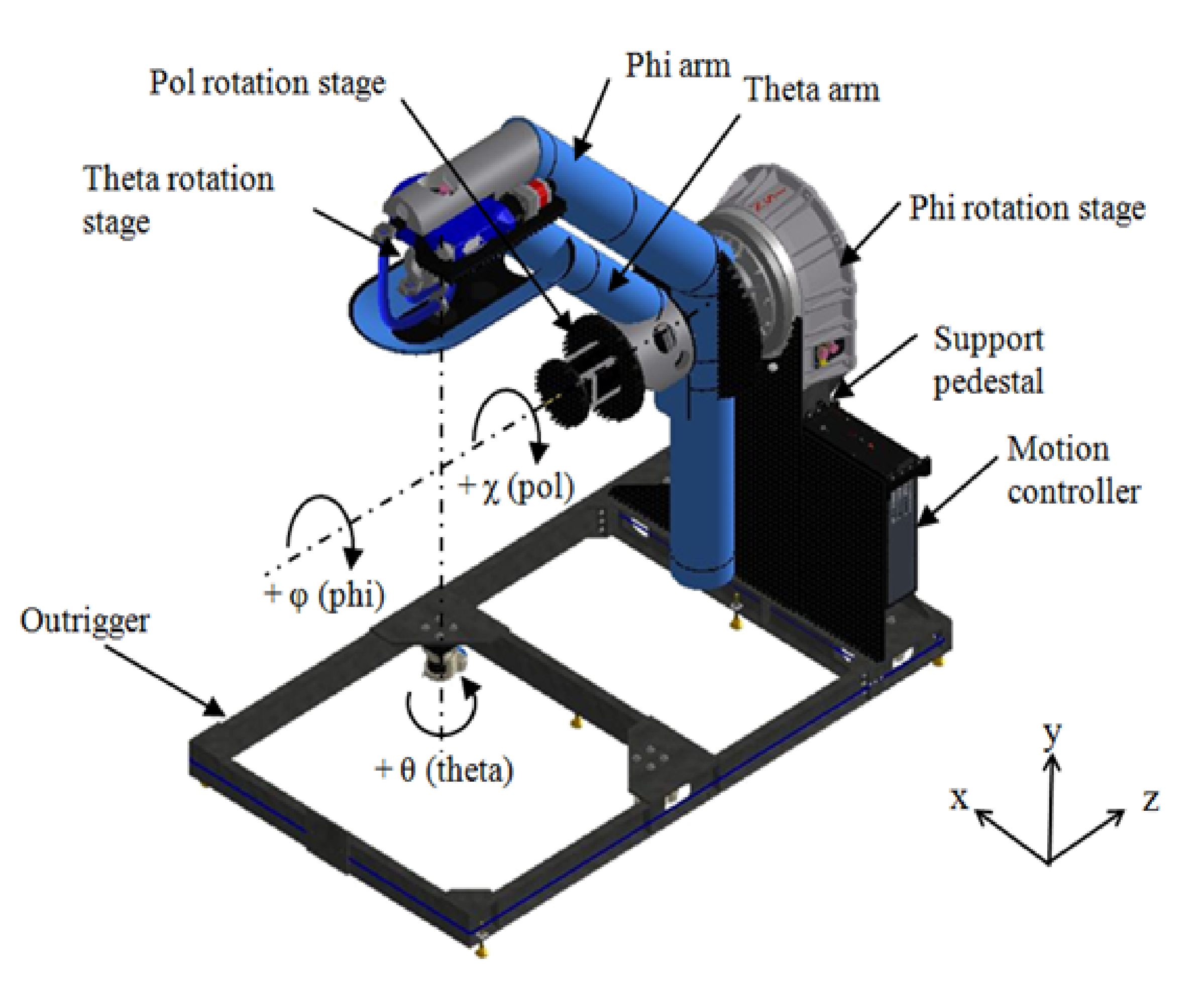
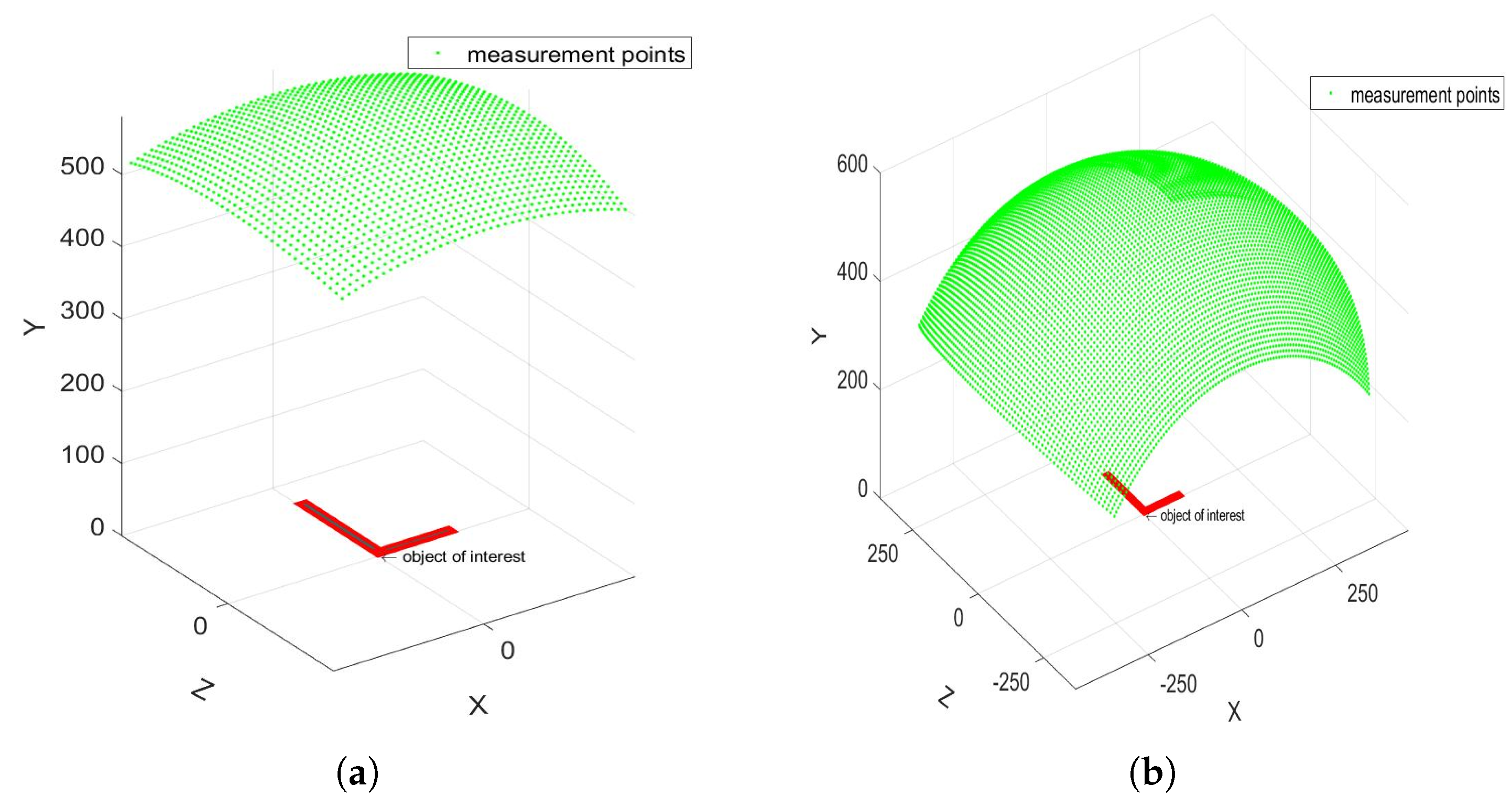
The spherical 3D-scanner is shown in Figure 1 and described more in detail by Nsengiyumva [15]. It is composed of a movable arm with $\theta$, $\varphi$, and polarization rotation stages. It is linked to a network analyzer acting as a continuous wave (CW) radar at single frequency measurements. Objects are placed on a Rohacell tower. We use a monostatic configuration, which corresponds to $S_{11}$ measurements. The probe antenna is a WR-10 standard gain horn that rotates above the object with a radius of 585 mm. The area covered by the scan depends on the settings in $\theta$ and $\varphi$. Here we use two scans: the small scan and the large one respectively defined as ${30}^{\circ }\times {30}^{\circ }$ and ${60}^{\circ }\times {60}^{\circ }$ as shown in Figure 2. The green points in Figure 2 span the field of view of the scanner. The scan step is ${0.2}^{\circ }$, which is slightly above the Shannon limit for processing measured data.We use the backpropagation of the fast Fourier transform algorithm to reconstruct the images of the objects of interest. Then, we obtain an image of the object being tested. A complete measurement including 3 frequencies takes 2 h. We aim at imaging objects at various frequencies, and polarization properties, since we know they are important diversity parameters for mmW imaging.

In the following we denote as $\mathrm{H}$ the horizontal polarization and as $\mathrm{V}$ the vertical one. They are defined as follows:

• $\mathrm{H}$: The electric field of the probe is parallel to Ox (see Figure 2) when $(\theta ,\varphi )=({90}^{\circ },{90}^{\circ })$;
• $\mathrm{V}$: The electric field of the probe is parallel to Oz (see Figure 2) when $(\theta ,\varphi )=({90}^{\circ },{90}^{\circ })$.

In a past study performed mainly by Migliaccio [17], we considered acquisitions at a single frequency 94 GHz. In this paper, we broadened the frequency range around the central frequency of 94 GHz, and afford the following three possibilities: 92, 94, and 96 GHz.

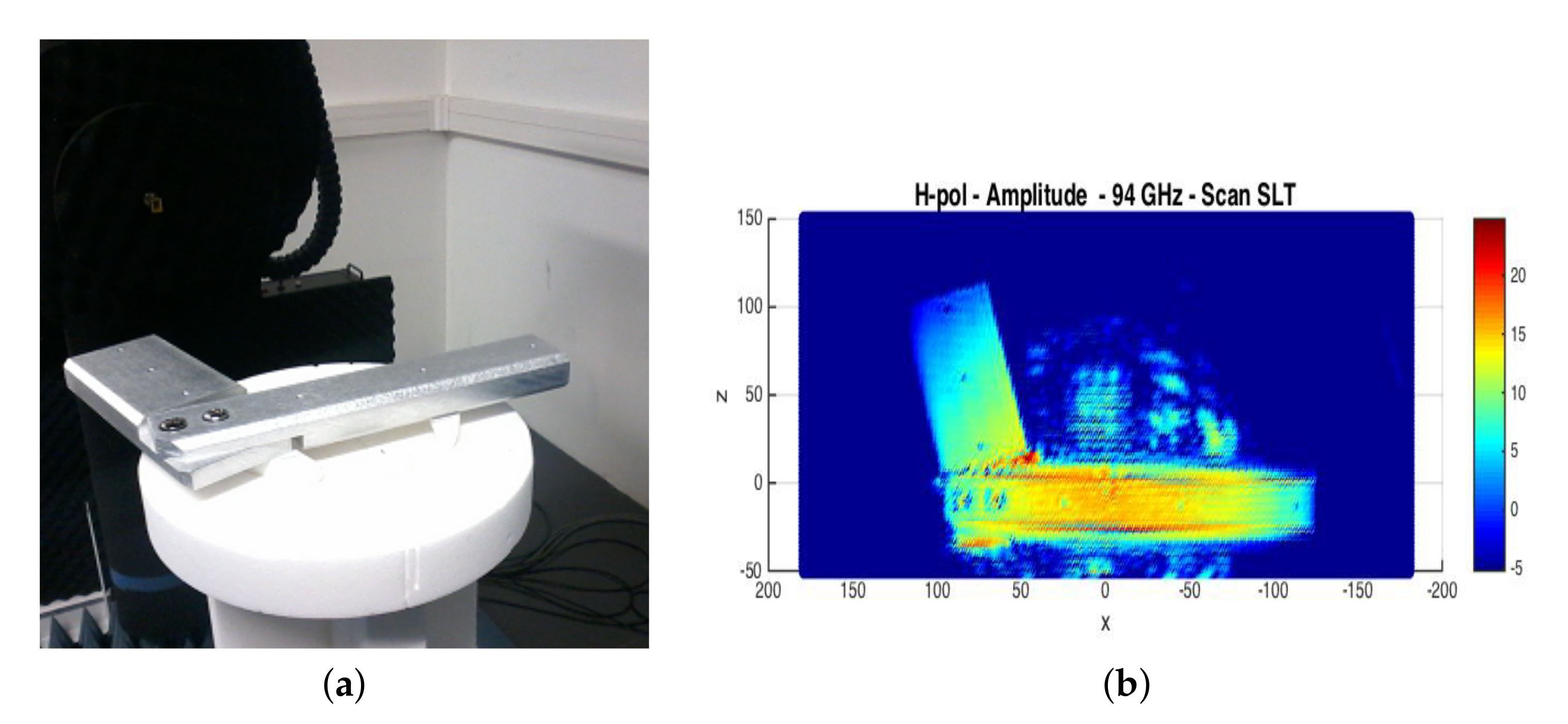
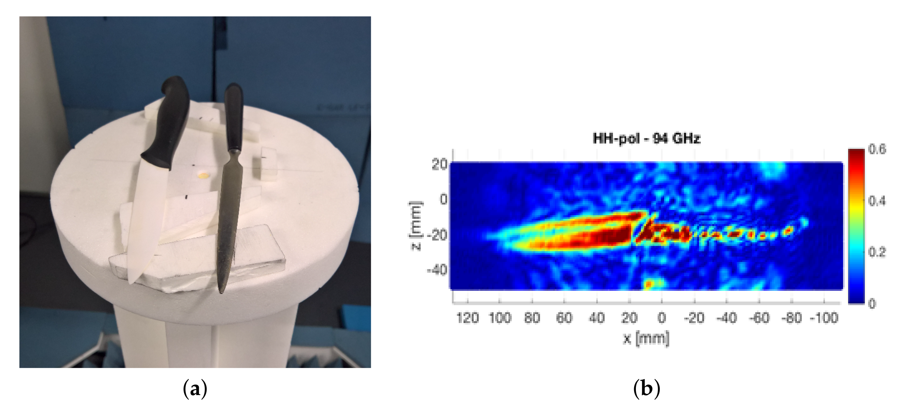
We display the scene and the acquired radar image (equivalently scan), obtained with frequency 94 GHz, and ‘$\mathrm{H}$’ polarization: Figure 3 shows the scene with a lethal object (a gun), and the corresponding scan. Figure 4 shows the scene with other examples of lethal objects (two knives), and the scan of one knife.

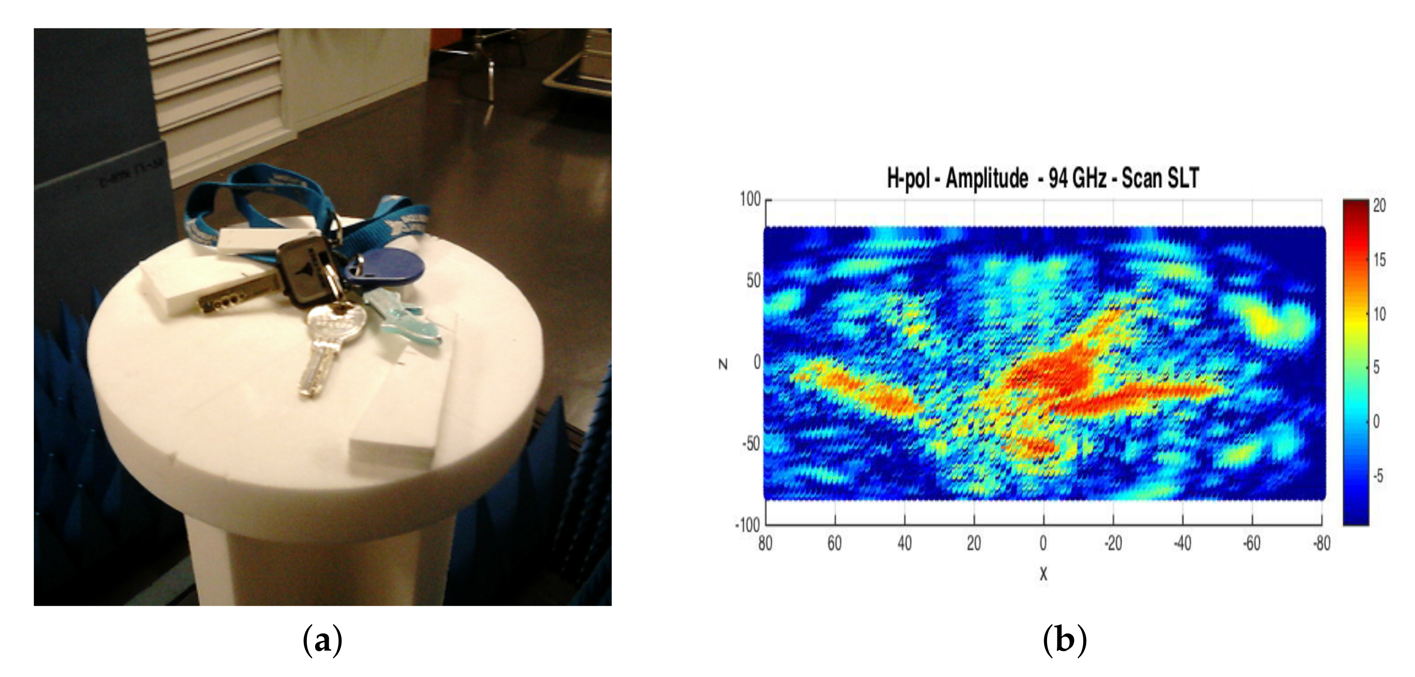
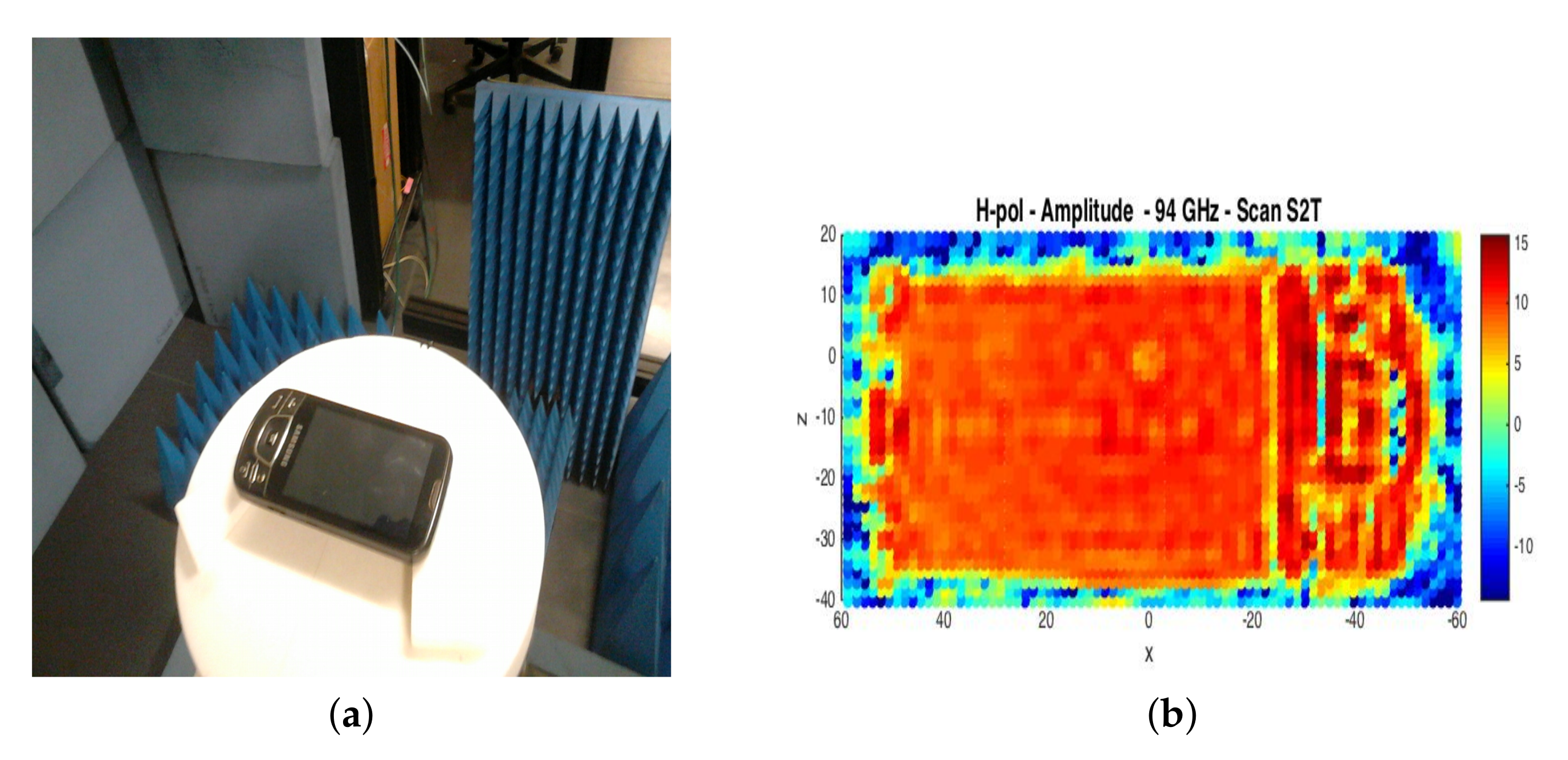
Figure 5 and Figure 6 show the scene and scans with non lethal objects (keys and smartphone). Moreover, Figure 7 shows the acquisition of a gun concealed under a jacket, with ‘$\mathrm{H}$’ polarization and frequency 94 and 96 GHz. We can notice that the contrast between the grip and the barrel is smaller in the 96 GHz image. This should be an advantage compared to the 94 GHz image because the region corresponding to the object of interest is homogeneous and easier to distinguish from the background. We can observe the significant difference in the aspect the reconstructed image when the frequency of the radar wave changes, and when we switch the polarization from ‘$\mathrm{H}$’ to ‘$\mathrm{V}$’. That is why both values of frequency and polarization will be taken into account in our joint tuning process. Other examples of acquisitions, with various polarization properties such as a fake gun concealed under a jacket are available in the paper from Migliaccio et al. [17].

As we had emphasized the possible interest of the combination of $\mathrm{H}$ and $\mathrm{V}$ polarization [17], a set of three possibilities will be included: ‘$\mathrm{H}$’, ‘$\mathrm{V}$’, and later on ‘$\mathrm{H}+\mathrm{V}$’, as explained in Section 2.5.

2.2. Image Segmentation, Feature Extraction and Object Classification

The image of the object being tested is a square 2D matrix, whose values are encoded on 8 bits, between 0 and 255. From such a matrix, a feature has to be extracted for the purpose of classification. Here are the steps of the image processing chain:

• the image values are scaled between 0 and 255 and a slight low pass filtering is applied to enhance the image.
• the Otsu threshold [28] is computed: A single grey level value is returned that separates pixels into two classes. This value, which is namely the Otsu threshold, is determined by minimizing intra-class intensity variance, or equivalently, by maximizing inter-class variance.
• the Otsu threshold is multiplied by a real value between 0 and 1, that will be called ‘factor’ in the rest of the paper. The image is binarized with the resulting value: the relevant pixels are set to 1, and the background to 0.
• The unexpected noisy pixels are removed with a mathematical morphology operation. Mathematical morphology tools have proven to be efficient in remote sensing applications, for instance by Sghaier et al. [29]. We combine namely an erosion followed by a dilation. For this, a structuring element with an appropriate size is required.

Starting from the binary image, we include several types of features which can be computed out of the segmented images: Histograms of Oriented Gradients (refer to the papers from Yan et al. [30], and Dalal et al. [31] (HOG), shape descriptors (sd) based on Fourier transform (refer to the paper from Slamani et al. [32]) -forming a vector of 10 components-, a scalar sphericity criterion created by Boughnim and two of the authors of the current paper [33], and a matrix signature dedicated to non star-shaped contours [33] (proposed by Bougnim et al. and denoted by Z in the following). We also included as a possibility the combination of sd, Z, and sphericity. To get this combination, we append vector sd, a columnwise vectorized version of Z, and the sphericity criterion. This yields a vector denoted by comb in the following. In summary, the feature extraction methods are sd, Z, and ‘comb’. HOG were left apart because of their elevated computational load.

A classification process is usually performed as follows: features compound a database which can be divided into a training, a validation, and a test set. These sets are always separated. The validation set, which is independent from the training set, is usually used for parameter selection/tuning. If several splits are performed between the training and the validation sets, the process is called ‘cross-validation’. The final result is the summation of all misclassified samples. A special case is ‘k-fold cross-validation’: the original set of samples is randomly partitioned into k equal-sized subsets. A single subset is retained as the validation data, and the remaining k-1 subsamples are used for training.

The test set is used to test the cross-validated classifier, whose parameters have been optimized. It is compound of images which have not been seen by the classifier during the cross-validation phase, but should however not be outliers. To classify objects out of radar images and the features computed from these images, we use an error code output classifier (ECOC) described by Dietterich et al. [37], and Escalera et al. [38] with k-fold cross-validation (see the paper from Anguita et al. [39] for details), with k = 10. That is, $90\%$ of the images are used for learning, and $10\%$ are used for validation. Then, for testing, we use unless specified approximately the same number of images as for validation.

The ECOC adresses a multi-class problem by dividing into several binary problems. Each class is associated with a bit string containing the features −1 and 1.

In the considered application we consider three classes. Their codewords is presented in

Table 1. Codeword generated by the ECOC classifier for each class.

Class	Codeword
class 1: guns	$\left\{1,1,0\right\}$
class 2: kives	$\left\{-1,0,1\right\}$
class 3: licit	$\left\{0,-1,-1\right\}$

. The set of three codewords compounds the codeword matrix.

ECOC basically converts a multi-class classification problem into a binary classification problem with the help of various coding schemes accompanied by a learner like Support Vector Machine (SVM). The basic idea is that the ECOCs help distinguish class labels by making them as dissimilar as possible. The error-correcting approach is inspired by communication problems: the identity of the correct output class for a given sample is being ‘transmitted’ through the image processing steps: binarization, feature extraction, and also learning process which may suffer from a limited number of samples, etc. This identity may then be corrupted during ‘transmission’. By encoding the class in an error-correcting code, the system may be able to recover from the errors (refer to the papers written by Dietterich et al. [37], and Windeatt et al. [40]). The ECOC estimates the category of a given sample by combining the outputs of several binary classifiers. The codeword matrix in Table 1 contains three columns, so we need three binary classifiers. It is also the reason why the Hamming distance between any codeword to another is 3. Longer codewords would yield a better separability between classes, but a larger number of binary classifiers.

We have chosen SVM as binary classifier: it handles correctly problems with relatively small datasets, even in nonlinear cases. The SVM maps the inputs to a high dimensional space where the differences between the classes can be revealed. It can avoid over-fitting automatically and has a high prediction accuracy, especially when the ‘kernel’ used to separate the classes is correctly chosen.

Given a training dataset of N samples which are vectors with P real components,

$S={\left\{({\mathbf{x}}_n,y_n)|{\mathbf{x}}_n\in \mathbb{R}P,y_n\in \left\{-1,1\right\}\right\}}_{n=1}^N$, we find the optimal hyperplane by solving the following problem:

$$\underset{\alpha }{max}[\sum _{n=1}^N{\alpha }_n-\sum _{n1,n2=1}^N{\alpha }_{n1}{\alpha }_{n2}{y}_{n1}{y}_{n2}Ker({\mathbf{x}}_{n1},{\mathbf{x}}_{n2})].$$

(1)

subject to:

$${\alpha }_n\ge 0\sum _{n=1}^N{\alpha }_n{y}_n=0.n=1,\dots ,N.$$

(2)

where $\alpha$ is a positive and real Lagrangian variable. The non zero Lagrangian variables ${\alpha }_n$ are called a support value or support vector. There are different types of kernel functions $Ker(.)$ such as the linear, polynomial or $rbf$ (radial basis function). More details can be found about kernels in the paper by Amari et al. [34]. Because the training datasets are suppossedly non-linearly separable, we include these three kernel functions as possible candidates. When the polynomial kernel is used, an additional parameter comes which is the degree. This parameter is not relevant for other kernels, and is therefore, for sake of simplicity, set to 3 as a recommended default value. A kernel always depends on a ‘scale’ parameter, and a basic parameter for any SVM is the ‘cost’ which yields a tradeoff between margin and misclassification of samples. The automatic selection of the cost and scale parameters is included in the optimization process that we propose. In the literature, a grid search is performed exhaustively on couples of values for the cost and the scale. That is, what is important is the order of magnitude of these values as mentionned by Duan et al. [35].

2.3. Adaptive Mixed Grey Wolf Optimizer for Parameter Selection

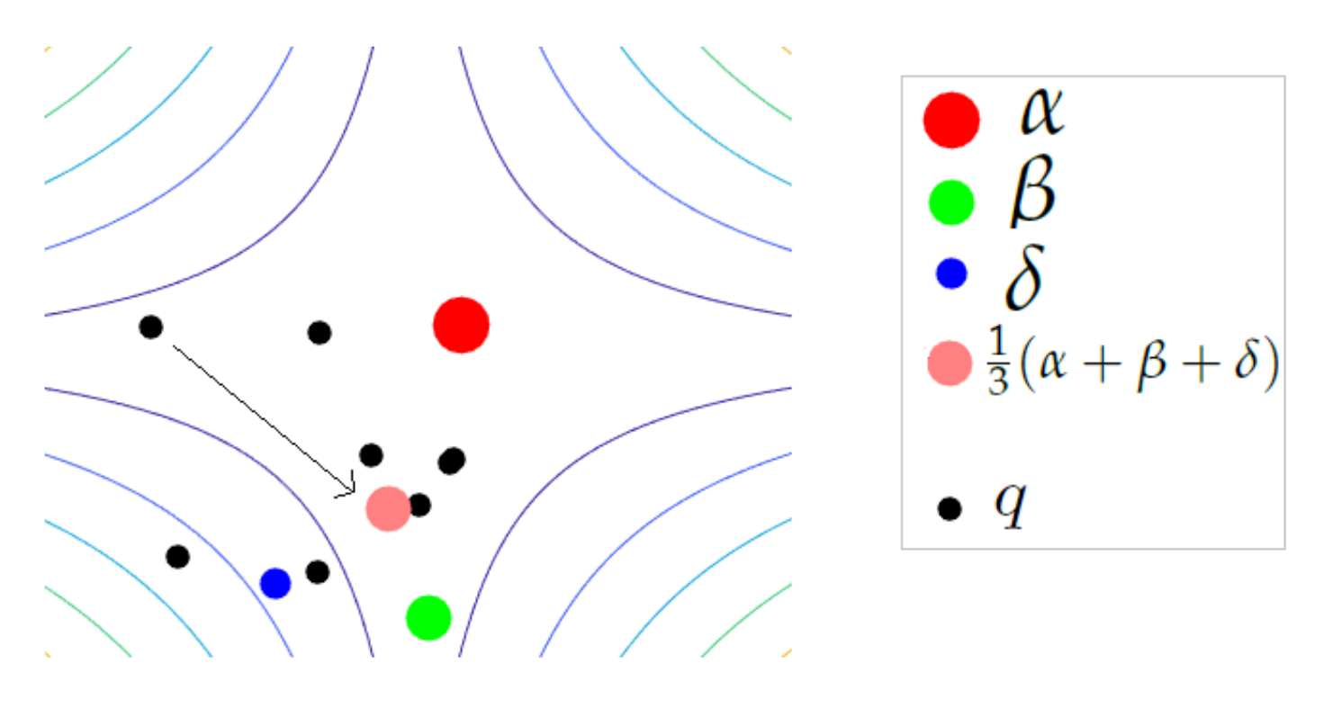
The optimization algorithms are computational techniques which find the optimal value (minimum or maximum) of what is called an ‘objective function’. In particular, meta-heuristics perform ‘trials’ of the objective function, to find iteratively and in the fastest manner the optimum of this objective function. The objective function is also called ‘criterion’. The grey wolf optimizer (GWO) proposed by Mirjalili et al. [18] is an iterative meta-heuristic inspired by the behaviour of grey wolves based on three leaders $\alpha$, $\beta$, $\delta$. In the original GWO, the search agents q, namely the wolves, evolve in a continuous search space, towards the center of mass of the three leaders. This is illustrated in Figure 8, where the search space is 2-dimensional and both parameters in a continuous search space.

When the search space is discrete, the center of mass of the three leaders may not belong to the search space. To tackle this problem, in the discrete version of the GWO proposed by Martin et al. [21], only one leader rules the displacement of a given wolf q at any iteration $\mathrm{iter}$, and the choice of the leader is alternated at random. Figure 9 illustrates the update rule for one wolve in the case of the discrete GWO: a given wolf q moves towards the leader $\alpha$ at a given iteration, and either towards $\beta$ or $\delta$ at some other iterations. The search space is 2-dimensional and both parameters in a discrete search space.

In addition to the three leaders $\alpha$, $\beta$, $\delta$, the discrete GWO may also involve two leaders 1 and 2 selected at random among the population of wolves.

The implementation of the GWO is based on a parameter denoted by a which varies from 2 to 0 across iterations $\mathrm{iter}=1,\dots ,T_{max}$. Exploration holds when $a>1$ and exploitation holds when $a\le 1$. Mirjalili et al. [18] propose a version of GWO where a decreases linearly. In a first version of the mixed grey wolf optimizer by Martin et al. [21], a parameter $\eta$ is introduced which turns a into a nonlinear function of the iteration index:

$$a=2(1-\frac{{\mathrm{iter}}^{\eta }}{{T_{max}}^{\eta }})$$

(3)

The probability of choosing any leader but $\alpha$ decreases proportionnally to a.

In the ‘adaptive’ mixed GWO (amixedGWO), we proposed to set:

$$a=\left\{\begin{array}{ccc}2(1-\frac{{\mathrm{iter}}^{\eta }}{{(T_{max}/2)}^{\eta }})& \mathrm{if}& \mathrm{iter}\le {\mathrm{T}}_{\max }/2\\ 2(1-\frac{{(\mathrm{iter}-T_{max}/2)}^{\frac{1}{\eta }}}{{(T_{max}/2)}^{\frac{1}{\eta }}})& \mathrm{if}& \mathrm{iter}>{\mathrm{T}}_{\max }/2\end{array}\right.$$

(4)

In Equations (3) and (4), $\eta$ is set by the user. In Equation (4) the expression of a depends on $\mathrm{iter}$, and is then adaptive, depending on whether the last iteration is far or close. If $\eta >1$, exploration is priviliged from $\mathrm{iter}=1$ to $\mathrm{iter}={\mathrm{T}}_{\max }/2$; in a second phase, from $\mathrm{iter}={\mathrm{T}}_{\max }/2+1$ to $\mathrm{iter}={\mathrm{T}}_{\max }$, exploitation is priviliged; but over all iterations, the same number of iterations is dedicated to exploration and to exploitation.

In the discrete GWO, the leader selection is performed as follows:

If $a>1$, the leader L is selected randomly among the $\alpha$, $\beta$, $\delta$, $\rho$1, and $\rho$2 wolves:

$$L=\left\{\begin{array}{ccccc}\alpha & \mathrm{if}& r\le \frac{a}{10}& & \\ \beta & \mathrm{if}& r>\frac{a}{10}& \mathrm{and}& r\le \frac{2a}{10}\\ \delta & \mathrm{if}& r>\frac{2a}{10}& \mathrm{and}& r\le \frac{3a}{10}\\ \rho 1& \mathrm{if}& r>\frac{3a}{10}& \mathrm{and}& r\le \frac{4a}{10}\\ \rho 2& \mathrm{if}& r>\frac{4a}{10}& \mathrm{and}& r\le \frac{5a}{10}\\ \alpha & \mathrm{if}& r>\frac{5a}{10}& \end{array}\right.$$

(5)

where r is a random value in $\mathbb{R}$, between 0 and 1.

If $a\le 1$, the leader is selected randomly among the $\alpha$, $\beta$, and $\delta$ wolves:

$$L=\left\{\begin{array}{ccccc}\alpha & \mathrm{if}& r\le \frac{a}{6}& & \\ \beta & \mathrm{if}& r>\frac{a}{6}& \mathrm{and}& r\le \frac{2a}{6}\\ \delta & \mathrm{if}& r>\frac{2a}{6}& \mathrm{and}& r\le \frac{3a}{6}\\ \alpha & \mathrm{if}& r>\frac{3a}{6}& \end{array}\right.$$

(6)

where r is a random value in $\mathbb{R}$, between 0 and 1.

As the parameter a is decreasing from 2 to 0 across the iterations, it is more and more probable for $\alpha$ to be selected as leader. The random wolves may be selected during the first part of the process, when $a>1$, and cannot be selected during the second part of the process, when $a\le 1$.

The MixedGWO and the variant amixedGWO can handle discrete and continous search spaces. In this work, we search 8 parameters in total. Among them, 7 parameters in discrete search spaces and 1 parameter in a continuous search space. Hence, these algorithms are particularly adequate to solve such a problem. We also have shown [21] that our amixedGWO is particularly adapted when the number of possibilities in the discrete search spaces is low. We will have, in the rest of this paper, to investigate on the ability of the amixedGWO to obtain the same results in terms of score than comparative methods, but with a lower number of iterations. Not only on simulations as we have done in [21], but also to solve a concrete problem of joint tunning of the parameters of a radar system.

2.4. Joint Parameter Tuning in a Real-World Radar System: Materials and Methods

The image acquisition hardware consists in a microwave emission and reception antenna. From these images, we wish to solve an inverse problem: we want to distinguish lethal objects from licit objects in radar acquisitions. For this, a machine learning algorithm is applied: an automatic process meant for image identification or classification. Both acquisition and classification involve parameters. The final purpose of this system is to classify objects, with the best possible results in terms of an adequate criterion. We propose to minimize this criterion with the amixedGWO.

In this subsection we present the classification process, showing examples of images, and examples of classification (more precisely cross-validation) results obtained with various sets of parameters.

We afford three classes: fake guns (class ‘1’), knives (class ‘2’), non lethal objects including key sets and smartphones (class ‘3’). As concerns the guns, half of the images were obtained from concealed objects. Unless specified, during cross-validation, we include in the image sets, for each class, 16 scans of best quality, i.e., those obtained close to the vertical axis with respect to the scene. As concerns class 1, 8 out of the 16 images are obtained from a fake gun concealed under a jacket; in class 2 we afford 16 acquisitions of knives; and in class 3 we afford 8 acquisitions from a set of keys, and 8 acquisitions from a smartphone.

In order for the classification algorithm to afford more images, we perform bootstrap (refer to a detailed description in the paper from Cameron et al. [41]): we generate additional images through subsampling, rotation, and translation. Eventually, the database is composed of $N=432$ images in total, that is, $N_1=N_2=N_3=144$ images for each class.

In the k-fold process, we choose $k=10$, which is a common practice. Therefore, this database is splitted into 10 subsets of 14 to 15 images for each class, selected randomly. One of these subsets is used for validation, and the nine other subsets are used for learning. $k=10$ experiments are performed, the tested images are always different from one experiment to another. In short, the software estimates a response for every image using the model trained without that image. In addition to the FRR which is a scalar criterion, the accuracy of the results obtained is measured through a confusion matrix. The confusion matrix contains the total number of images, summated over the $k=10$ experiments, for each label of origin (along rows) and label attributed by the classifier (along columns). So we get a $3\times 3$ confusion matrix for each classification trial. All algorithms were implemented in MATLAB R2020a and run on an Intel Core i5 2.5 GHz CPU with 4 GB RAM (Random Access Memory).

In Section 2.4.1 we present examples of processed images, and in Section 2.4.2, we provide classification results in cross-validation experiments with various parameter values.

2.4.1. Examples of Processed Images

The acquired radar images have an original size of $1024\times 1024$ pixels. They are subsampled to size $256\times 256$. After binarization, erosion and dilation are applied, with some structuring element (see Section 2.2). Due to the a priori unknown shape of the object of interest, we have chosen a structuring element with vertical and horizontal axes of symmetry: a square, whose size (number of pixels × number of pixels) is one of the parameters optimized by our amixedGWO.

In practice this size parameter depends on the size of the image. For an image with two times more rows and columns, the size of the structuring element would also be multiplied by two. The larger the structuring element, the more noisy pixels are removed, but the larger is the modification of the shape of the object of interest.

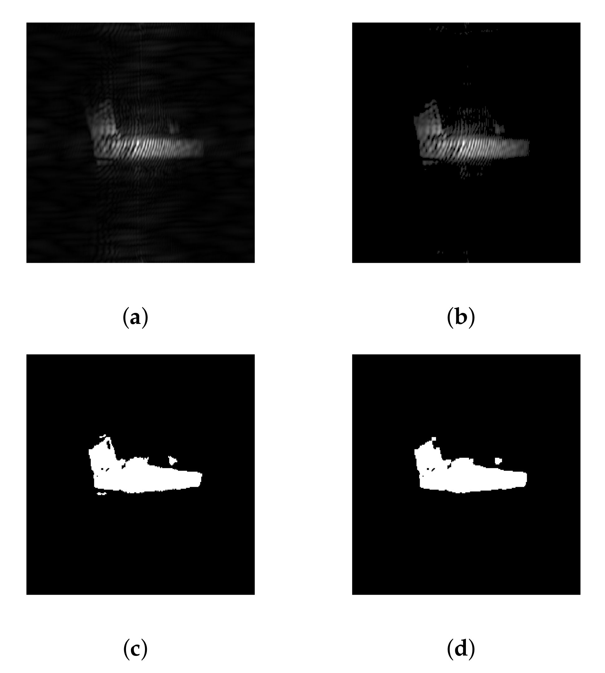
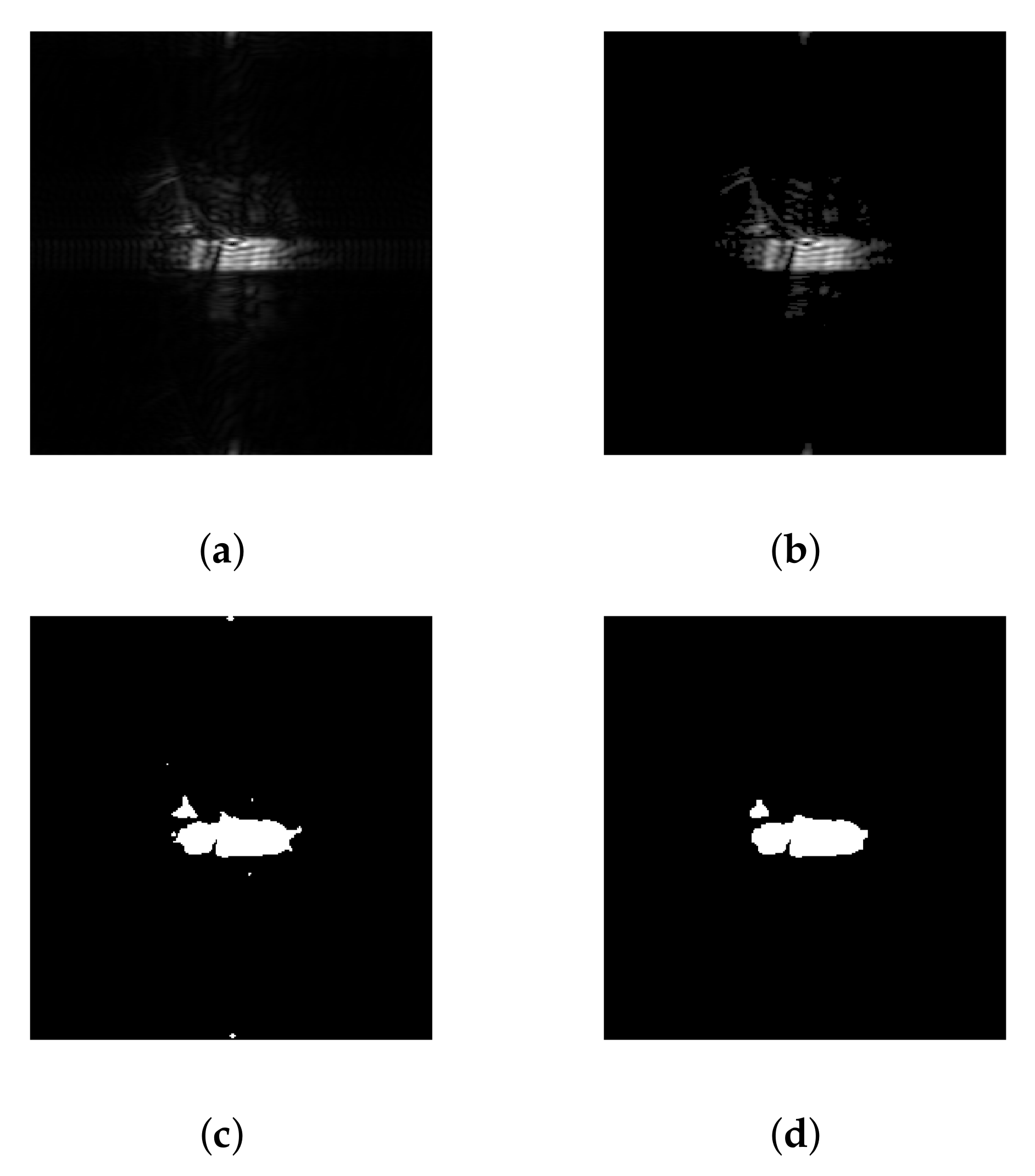
As an example, we illustrate the image processing chain with the same concealed gun as in Figure 7. In Figure 10 and Figure 11, we illustrate the steps of image processing (refer to the enumeration in Section 2.2). Figure 10 results from an acquisition at frequency 94 GHz and Figure 11 at 96 GHz. In each case, in Figure 10 and in Figure 11 as well, (a) is the input grey level image, (b) the enhanced image, (c) the image binarized with a scaled Otsu threshold, and (d) the output of mathematical morphology operations, aiming at removing parasite pixels. A careful comparison of the images permits to notice that the contrast is slightly better in (b) than in (a), and that some parasites present in (c) are no longer present in (d). We also clearly notice the difference between the acquisitions at 94 and 96 GHz. As mentionned in Section 2.1, the contrast between the two parts of the gun (grip and barrel) is too large in the 96 GHz image to integrate them in the same class. The pixels of the grip are mostly integrated in the background and not in the object of interest. The 94 GHz image yields a better segmentation result. This comment may not be valid for all types of objects but permits to grasp the influence of the frequency in our overall classification process.

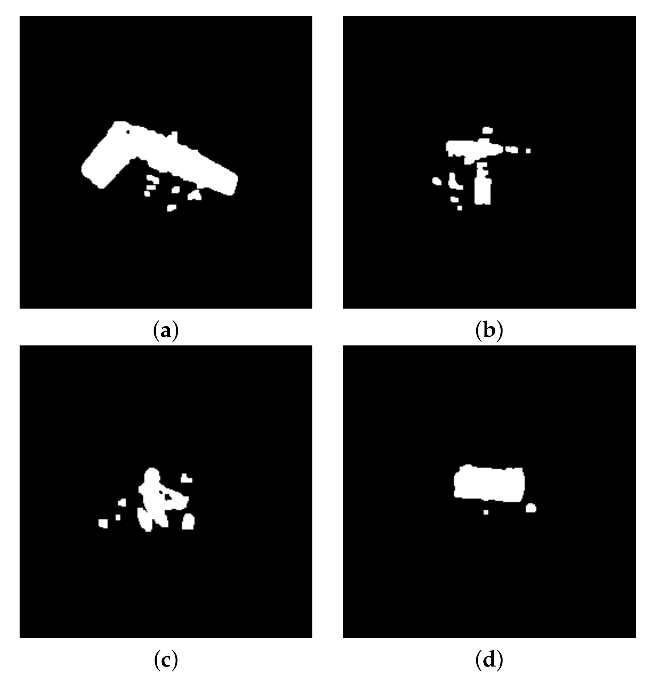
For various objects, not only a gun but also a knife, a set of keys, and a smartphone, a segmentation result is illustrated in Figure 12. The Otsu threshold has been multiplied by 0.87 to get this binarization result. The size of the structuring element is 4.

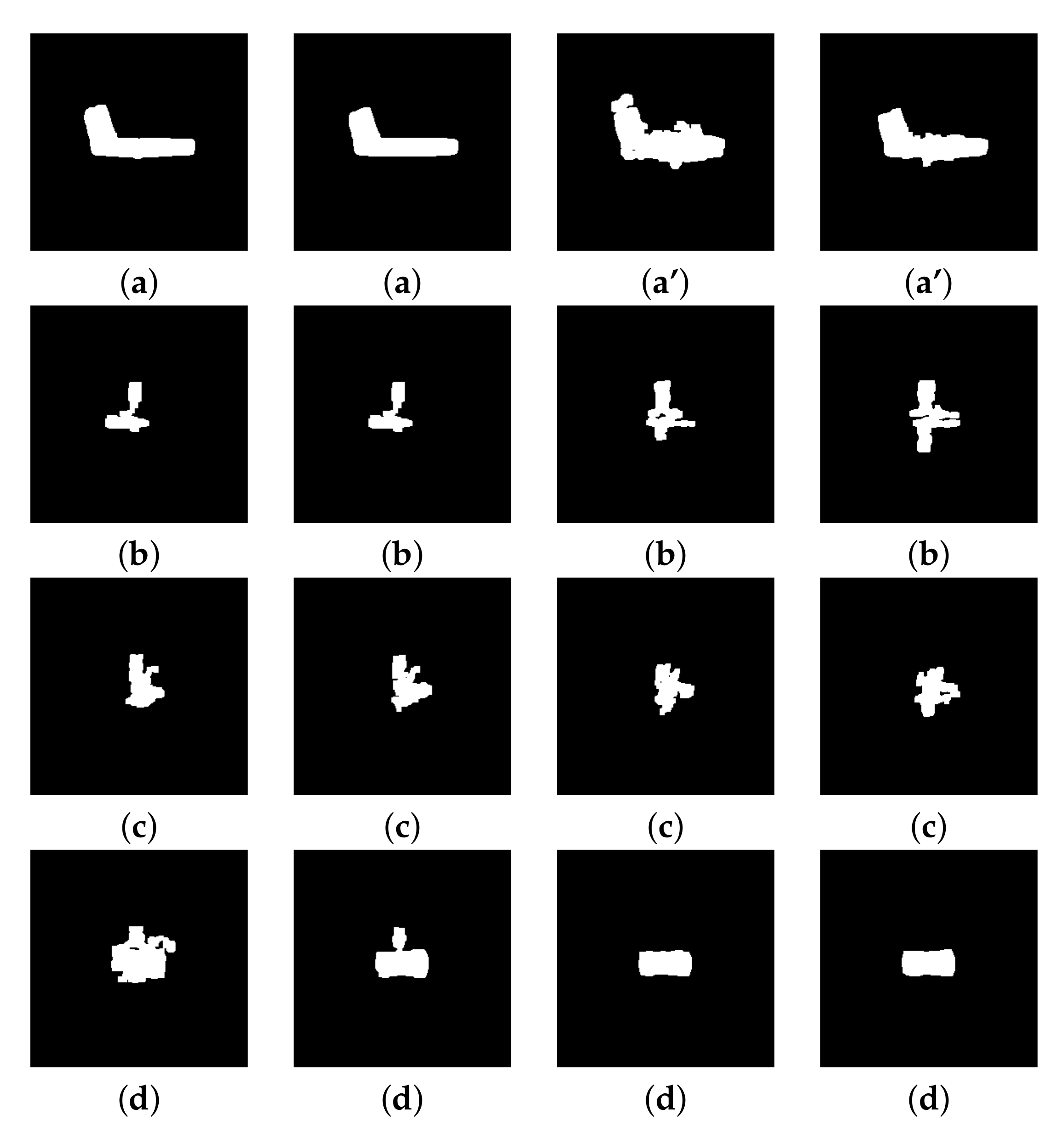
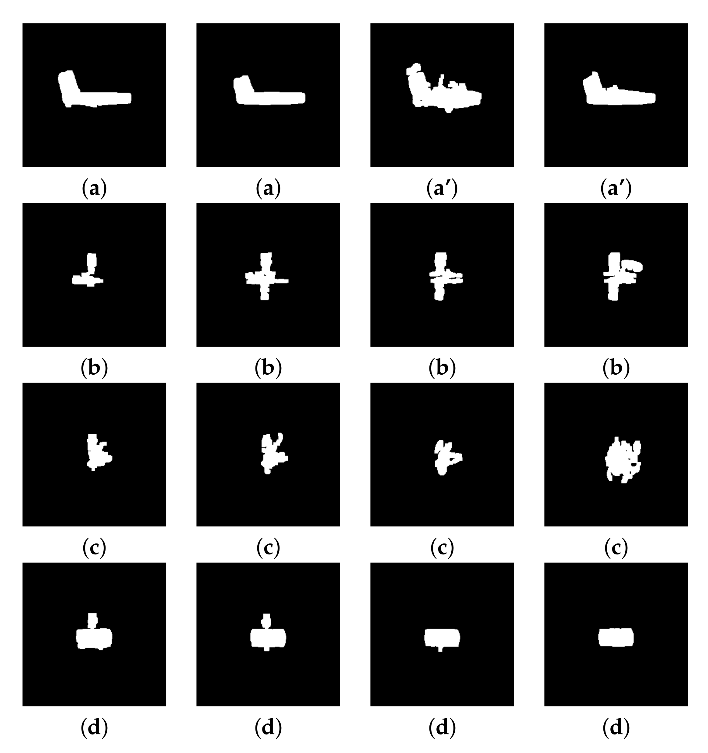
Figure 13 presents additional results of image acquisition and processing with this same threshold and size of structuring element. And Figure 14 presents additional results of image acquisition and processing, also at 94 GHz, but with ‘$\mathrm{H}+\mathrm{V}$’ polarization, threshold value 0.59, and 2 pixels for the size of the structuring element. In Figure 13a’ and Figure 14a’ the segmentation resulting from a concealed gun is presented. It is worth noticing that, to get the ‘$\mathrm{H}+\mathrm{V}$’ images, a whole sequence of image processing with eventually a binarization is performed on an ‘$\mathrm{H}$’ acquisition, a ‘$\mathrm{V}$’ acquisition, and that the ‘$\mathrm{H}+\mathrm{V}$’ image is the result of the combination of the binary images resulting from the ‘$\mathrm{H}$’ acquisition and the ‘$\mathrm{V}$’ acquisition. Consequently, to get an ‘$\mathrm{H}+\mathrm{V}$’ image, the computational load which is dedicated to acquisition and creation of the binary image is roughly two times higher than for either an ‘$\mathrm{H}$’ or a ‘$\mathrm{V}$’ image.

Here are some figures concerning the computational load for image processing and classification:

We remind that we afford 432 images in total. The total computational load for each step is computed as follows:

• firstly to get the segmented images: the load of the data lasts 17.1 s, the segmentation and creation of the descritors out of the loaded images lasts 16.7 s. This yields about 33.8 s. to generate the predictors (the features which are provided to the classification algorithm) for all images. This computational time may vary from 30 to 35 s. depending on what descriptor is used (either $\mathbf{sd}$, Z, or $\mathbf{comb}$). So the mean value for one image is $7.8\times {10}^{-2}$ s.
• secondly to train the classifier, that is, essentialy, transform the data into orthogonal codes: $4.8\times {10}^{-2}$ s. So the mean value for one image is $1.1\times {10}^{-4}$ s.
• thirdly to perform cross-validation with k-fold process: $3.8\times {10}^{-1}$ s. So the mean value for one image is $8.9\times {10}^{-4}$ s.
• fourthly to compute the accuracy from the cross-validated classifier: $4.3\times {10}^{-2}$ s. So the mean value for one image is $1.0\times {10}^{-4}$ s.

In total, for the load, segmentation, descriptor creation and cross-validation, the required time is 34.2 s, that is, a mean value of $7.9\times {10}^{-2}$ s for one image.

The figure which is however the most relevant is the time required if we just want to make a prediction for one image, that is, perform segmentation and computation of the descriptor, and ask the already trained classifier to estimate the class the image belongs to. The time for this is $7.8\times {10}^{-2}$ s for the segmentation, in addition to $5\times {10}^{-4}$ s for the prediction, which yields in total $7.85\times {10}^{-2}$ s.

We notice that the computational time is essentially dedicated to the segmentation and computation of the descriptor. The time dedicated to the prediction is negligible. As it is less than ${10}^{-1}$ s, it can be considered as real-time.

Figure 13 presents 16 of the segmented images obtained from a ‘$\mathrm{V}$’ polarization, at frequency 94 GHz. All the 432 images, including these 16 images, are available as png images at the following links: [42] (rar format), [43] (zip format). The 16 ‘$\mathrm{H}$’ scans for each class are also available.

2.4.2. Examples of Classification Results

A classification algorithm is generally evaluated through a ‘false recognition rate’ (FRR) criterion. It is defined as:

$$FRR=100\frac{M_1+M_2+M_3}{N_1+N_2+N_3}$$

(7)

where, for class $c=1,\dots ,3$, $M_c$ is the number of misclassified images, and $N_c$ is the total number of images considered for classification.

In this study, we also use as a relevant criterion the number of missclassified images.

To illustrate some classification experiments obtained with the cross-validation database, we fixed the parameters as follows:

• radar wave polarization: ‘$\mathrm{H}+\mathrm{V}$, ‘$\mathrm{H}$, or ‘$\mathrm{V}$;
• radar wave frequency: 94 or 96 GHz;
• factor multiplying an Otsu threshold: 0.1 to 0.8;
• size of the structuring element: 4;
• type of feature: $\mathbf{sd}$;
• type of kernel: polynomial;
• scale for the kernel: 1 to 1000;
• cost C: 100.

So we intentionnaly vary 4 out of the 8 parameters: some preliminary experiments have proven the sensitivity of the classification results on these parameters.

Table 2. Number of missclassified images for various conditions for the acquisition and the procecessing of the radar images.

	(Polarization, Frequency)	(H+V, 94)	(H, 94)	(V, 94)	(H+V, 96)	(H, 96)	(V, 96)
(Threshold Factor, Scale)
(0.1, 1000)		167	195	267	125	125	191
(0.2, 100)		37	43	53	67	53	76
(0.4, 10)		6	7	5	32	17	23
(0.6, 1)		0	1	2	1	10	4
(0.8, 10)		5	5	6	11	14	9

shows that the results in terms of FRR are mostly correlated with the image processing parameters: if they are correctly chosen, we may choose either a polarization, or another, knowing that ‘$\mathrm{H}$’ or ‘$\mathrm{V}$’ yield a smaller computational time compared to ‘$\mathrm{H}+\mathrm{V}$’. We also may choose either a frequency or another. This facilitates the design of the acquisition setup and reduces the acquisition time. From these preliminary experiments, we deduce that it is of a certain interest to estimate the best set of parameters with an adequate computational technique. The purpose of the next subsection is to show how the parameters mentionned above are included in search spaces for the amixedGWO, and how a classification experiment can be considered as a trial of an objective function in the paradigm of this optimizer.

2.5. Criterion and Search Spaces for the Adaptive Mixed Grey Wolf Optimizer

The criterion is the FRR, which should be as small as possible. There exists two parameters for the radar image acquisition system, and six parameters for the image processing algorithms. All these parameters take their values in discrete search spaces, except one, the factor multiplying the Ostu threshold (see Section 2.4.2).

All the radar acquisitions are performed in advance, with all the candidate values of polarization and frequency that we have chosen. To create the ‘$\mathrm{H}+\mathrm{V}$’ configuration considered in the previous study by Migliaccio et al. [17], the ‘$\mathrm{H}$’ and ‘$\mathrm{V}$’ acquisitions are combined ‘online’, that is, during one test in the optimization process. The ‘$\mathrm{H}+\mathrm{V}$’ image is the binary summation of the result of segmentation and binarization applied to ‘$\mathrm{H}$’ on the one side and ‘$\mathrm{V}$’ on the other side.

The polarization and frequency values are naturally ‘discrete’ parameters.

The third parameter is a real value, larger than or equal to 0 and less than or equal to 1. This is a factor involved in the binarization of the images: it multiplies a threshold value computed automatically from a given image with the Ostu method.

The fourth parameter is the size (in integer number of pixels) of the squared structuring element used to remove parasite pixels from the thresholded image. There exist a naturally finite number of candidate ‘features’ also called descriptors, composing a discrete set of values (fifth parameter). As sixth parameter, three possible kernels are available for SVM (linear, rbf, and polynomial).

The seventh and eighth parameters are the scale and cost used in the SVM-ECOC classification algorithm. As only their order of magnitude is important, we chose a set of discrete candidate values, powers of 10 between 1 and 1000.

The amixedGWO seeks the best solution in terms of FRR, or equivalently in terms of number of misclassified images.

Table 3. Search spaces for adaptive mixed GWO optimizer: parameter index vs. search space properties.

i	${\mathit{H}}_{\mathit{i}}$	${\mathbf{d}}_{\mathit{i}}^{\mathit{val}}$
1	3	${\left[\mathrm{H},\mathrm{V},\mathrm{H}+\mathrm{V}\right]}^T$
2	2	${\left[94,96\right]}^T$
3		${\left[0\dots 1\right]}^T$
4	4	${\left[1,2,4,6\right]}^T$
5	3	${\left[\mathbf{sd},\mathrm{Z},\mathbf{comb}\right]}^T$
6	3	${\left[\mathrm{linear},\mathrm{rbf},\mathrm{polynomial}\right]}^T$
7	4	${\left[1,{10}^1,{10}^2,{10}^3\right]}^T$
8	4	${\left[1,{10}^1,{10}^2,{10}^3\right]}^T$

describes the search spaces for the parameters presented above. We use the same notations as in our previous work with Martin [21]. For each parameter index i∈${\left[1,\dots ,8\right]}^T$, $H_i$ is the number of possible values, and ${\mathbf{d}}_i^{\mathit{val}}$ a vector containing their values. The value $H_i$ is not relevant for the threshold parameter, which belongs to a continuous search space.

In the considered application, a trial of the objective function consists in:

• selecting a set of images acquired with given frequency and polarization values;
• binarizing the images with some threshold value;
• removing parasite pixels with a mathematical morphology operator of a given size;
• computing some features;
• applying the classification process out of these features with some kernel, scale and cost in SVM.

An example of set of parameters for a given ‘trial’ can be for instance $\mathbf{x}=[\mathrm{V},94,0.5,2,\mathrm{Z},$${\mathrm{linear},100,1000]}^{\mathrm{T}}$.

x is a vector containing all the required information for a trial yielding an FRR value. To find out the best set of parameters in terms of FRR, the advantage of a computational technique, namely the amixedGWO, with respect to an exhaustive search is two-fold:

Firstly, we notice that an exhaustive search requires the discretization of the search space for the threshold parameter, which is in itself an approximation. In an arbitrary manner, let’s select 10 possible values for this search space.

Secondly, let’s compute the number of runs $R^{es}$ which would be required by an exhaustive search of all possible combinations of parameter values: $R^{es}=H_1\times H_2\times H_3\times H_4\times 10\times H_6\times H_7\times H_8=3\times 2\times 10\times 4\times 3\times 3\times 4\times 4$; which yields $R^{es}$ = 34,560. This number will be compared in the following with the number of runs required by the amixedGWO.

3. Results and Discussion

This section presents a description of the experimental resultsobtained by amixedGWO and comparative optimization algorithms: firstly on simulations, and secondly on experimental radar data. Section 3.1 aims at validating the proposed approach on a synthetic test function, with search spaces which are equivalent to our real-world application. Section 3.2 applies the proposed approach on experimental radar data. Section 3.3 discusses the results and how they can be interpreted.

3.1. Comparative Performance Evaluation on a Synthetic Objective Function

To ensure the adequacy of the amixedGWO for the considered system design issue, we have tested the amixedGWO on a simplified function which models our problem: a function of 8 variables, whose minimum value is 0. A Matlab© implementation of the amixedGWO and comparative methods such as GWO (grey wolf optimizer from Mirjalili et al. [18]), PSO (particle swarm optimization from Eberhart et al. [24]), TSA (tree seed algorithm from Kiran et al. [19]) and CGSA (chaotic gravitational search algorithm from Mirjalili et al. [20]) is available as a toolbox, at the following link: [44]. The objective function used as ‘surrogate’ (or equivalently a model) for this problem is a combination of hyperbolic tangent functions. It is denoted by $F:\mathbb{R}8\mapsto \mathbb{R}$. Let $x={\left[{\mathbf{x}}_1,{\mathbf{x}}_2,\dots ,{\mathbf{x}}_8\right]}^T$. The components of x are accessed as ${\mathbf{x}}_1$, ${\mathbf{x}}_2$, …, ${\mathbf{x}}_8$.

Let ${\mathbf{x}}^1={\left[1,1,0.88,2,2,3,100,1000\right]}^T$, be a first vector containing the ‘expected’ values.

Let ${\mathbf{x}}^2={\left[2,2,0.68,2,1,1,10,100\right]}^T$, be a second vector containing a second set of ‘expected’ values.

Let $\mathbf{g}\mathbf{1}\left(\mathbf{x}\right)=|\mathbf{x}/10|$, and $\mathbf{g}\mathbf{2}\left(\mathbf{x}\right)=|sin(3\ast tanh\left(\right|\mathbf{x}\left|\right)\left)\right|$. sin is the sine function, and tanh is the hyperbolic tangent function. $\mathbf{g}\mathbf{1}$ and $\mathbf{g}\mathbf{2}$ are vectors of same length as x.

Let $\underline{{\mathbf{x}}^1}=\frac{\mathbf{x}-{\mathbf{x}}^1}{{\mathbf{x}}^1}$ and $\underline{{\mathbf{x}}^2}=\frac{\mathbf{x}-{\mathbf{x}}^2}{{\mathbf{x}}^1}$.

Let

$$\mathbf{g}\left(\mathbf{x}\right)=30(\mathbf{g}\mathbf{1}\left(\underline{{\mathbf{x}}^{\mathbf{1}}}\right)\circ \mathbf{g}\mathbf{1}\left(\underline{{\mathbf{x}}^2}\right)+\mathbf{g}\mathbf{2}\left(\underline{{\mathbf{x}}^1}\right)\circ \mathbf{g}\mathbf{2}\left(\underline{{\mathbf{x}}^2}\right))$$

(8)

$\mathbf{g}\left(\mathbf{x}\right)$ is a vector of same length as x, and the $i\mathrm{th}$ component of g depends only on the $i\mathrm{th}$ component of x.

Then we define:

$$F\left(\mathbf{x}\right)=\sum _{i=1}^8{\mathrm{g}}_{\mathrm{i}}\left({\mathbf{x}}_{\mathrm{i}}\right)$$

(9)

Here are some properties of this function:

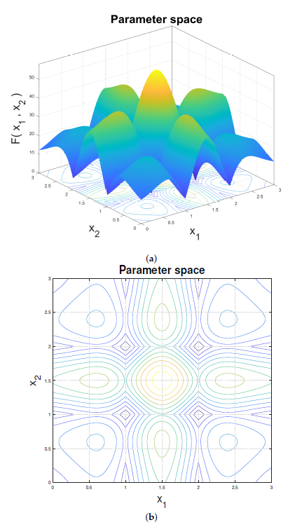
Obviously, $F\left(\mathbf{x}\right)\ge 0$, and $F\left(\mathbf{x}\right)=0$ if $x={\mathbf{x}}^1$ or if $\mathbf{x}={\mathbf{x}}^2$. That is, F exhibits, among others, two local zero-valued minima at the locations ${\mathbf{x}}^1$ and ${\mathbf{x}}^2$. F exhibits in total 8 zero-valued minima: 4 at locations ${\left[{\mathrm{l}}_1,{\mathrm{l}}_2,0.88,2,2,3,100,1000\right]}^T$, and 4 at locations ${\left[{\mathrm{l}}_1,{\mathrm{l}}_2,0.68,2,1,1,10,100\right]}^T$, where the couple $\left\{{\mathrm{l}}_1,{\mathrm{l}}_2\right\}$ take the 4 possible combinations of values 1 and 2. As it exhibits several local minima, $F\left(\mathbf{x}\right)$ is called a ‘multimodal’ function. In Figure 15, we display its variations as a function of the two first variables ${\mathbf{x}}_1,{\mathbf{x}}_2$ only, the six last variables being set to the expected values ($0.88$, 2, 2, 3, 100, and 1000). The local minima are visible in Figure 15, at $\left(1,1\right)$, $\left(1,2\right)$, $\left(2,1\right)$, and $\left(2,2\right)$. The maximum value is only around 50 because the chosen values for the six last variables for the plot yield small values for F.

When an optimization algorithm is run to minimize a function, the final value obtained, at the location which is considered by the algorithm as the best one, is called a ‘score’. Also, the value, at each iteration, of the best score obtained up to this iteration, is stored in what is called a ‘convergence curve’.

When the adaptive mixed GWO is run, we set the values of $H_i$ as in Table 3 for all i. The amixedGWO and comparative algorithms are applied to minimize the objective function with 6 search agents, and 20 iterations. In amixedGWO, parameter $\eta$ is set to 2, after some preliminary experiments.

To assess the statistical performances of these five optimization methods, we performed 10 experiments, for the same objective function F.

We remind that for a method to be better than the others, it has to exhibit the smallest score and a convergence curve which is below the other curves, as mentionned in the work of Mirjalili et al. [18], and the work of Martin et al. [21]. Depending on the final application, the computational load required for a given iteration may also be relevant. The computational time required to run six times the objective function F (for the six agents at any iteration), is $2.4\times {10}^{-5}$ s. Excluding this time, the computational time required for one iteration of the optimization algorithms are as follows: $2.07\times {10}^{-3}$ for amixedGWO, $7.00\times {10}^{-5}$ for PSO, $9.30\times {10}^{-5}$ for GWO, $9.43\times {10}^{-4}$ for TSA, $7.39\times {10}^{-4}$ for CGSA. These figures show that the amixedGWO is slower than any other algorithm. PSO is the fastest; TSA and CGSA are about two times faster than amixedGWO. Some other experiments have shown that amixedGWO outperforms TSA in terms of speed as soon as the number of agents is larger than 60, but we aim at keeping the number of agents as small as possible for the considered application. We also have to keep in mind that this figure is relevant for applications where the time required for one run of the objective function is small compared to the computational time required by the optimization method itself. We will check further in the paper that this is not the case for the application considered here.

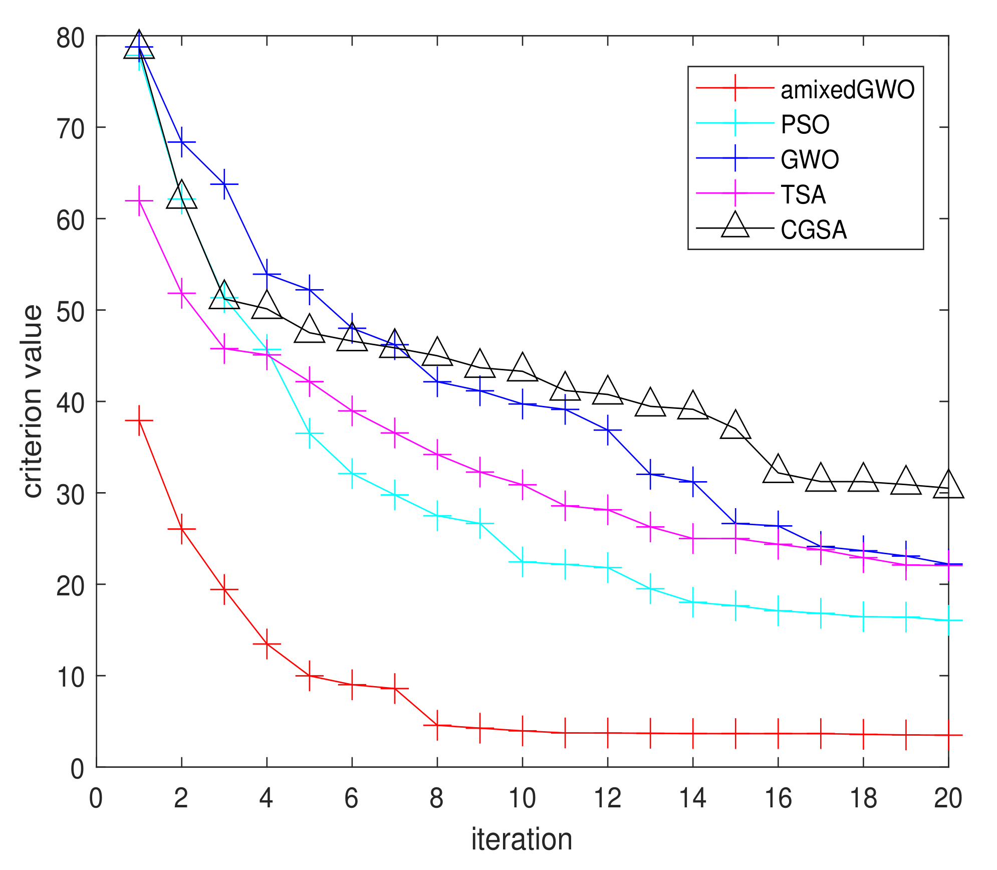
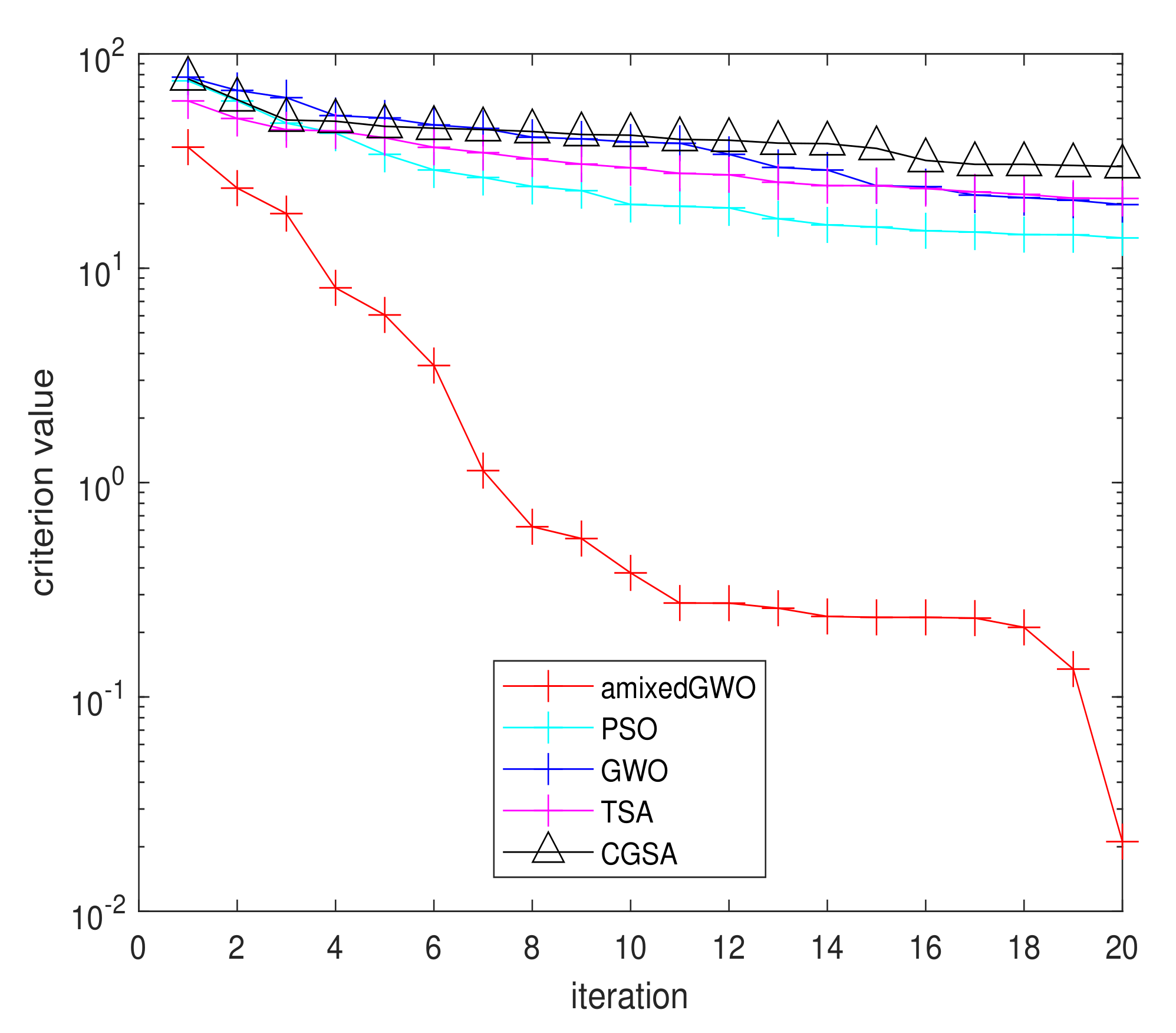
In Figure 16 (resp. Figure 17) we display the arithmetic (resp. geometric) mean, over all experiments, of the convergence curves obtained by amixedGWO, PSO, GWO, TSA, and CGSA.

Figure 16 shows that, although the inital values are elevated, all methods except CGSA drop below 30. The proposed amixedGWO reaches quickly a value which is below 10 (at the fifth iteration). On the contrary, the comparative methods hardly reach 15, even at the last iteration. Figure 17 permits to observe in detail how the proposed method behaves after the fifth iteration: the criterion value is reduced progressively, to reach a geometric mean of 0.27 (corresponding to an arithmetic mean of 5.5). We infer from the convergence curve of amixedGWO that the optimal values of the discrete parameters are found quickly, and that the amixedGWO has time to refine the estimate of the continuous parameter.

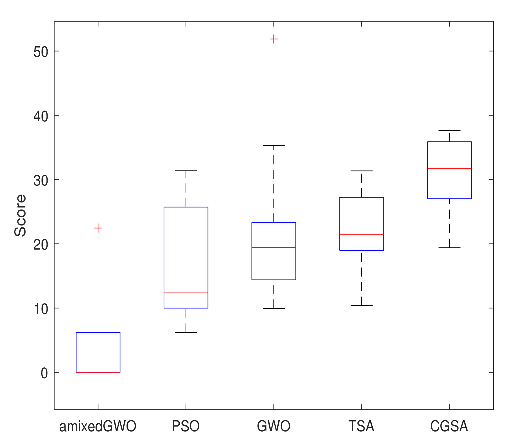
We display in Figure 18a box plot for the final scores, over all the experiments, of all algorithms. On each box, the central mark indicates the median, and the bottom and top edges of the box indicate the 25th and 75th percentiles, respectively. The whiskers extend to the most extreme data points not considered outliers, and the outliers are plotted individually using the red ‘+’ symbol.

We remind that we expect these methods to provide the least possible value. We notice that, in Figure 18, all marks of amixedGWO are below the others, in particular the median score. More precisely, the amixedGWO outperforms the comparative methods in terms of the figures, computed on all score values, presented in

Table 4. Relevant figures computed over all experiments for all comparative methods on the obtained final scores: arithmetic mean, geometric mean, minimum value.

	Methods	amixedGWO	PSO	GWO	TSA	CGSA
Figures
arithmetic mean		3.49	16.05	22.21	22.04	30.50
geometric mean		2.11 × 10−2	13.84	19.80	21.15	29.79
minimum value		1.00 × 10−5	6.19	9.93	10.37	19.38

.

Table 4 shows that the amixedGWO outperforms by far the comparative methods for all these relevant figures. PSO and GWO are the second and third algorithms. The box plot shows however that the variability on the results provided by PSO is more elevated than for GWO method. As the values of $H_i$ are the same in the real-world application, we expect the amixedGWO to find reliably the expected parameter values in our radar system design.

3.2. Joint Parameter Tuning in a Real-World Radar System: Results

In this subsection we provide the results obtained by amixedGWO and comparative optimization algorithms while selecting the best parameters for image classification. This is done on multiple ‘cross-validation’ experiments.

In Section 3.2.1 we show how amixedGWO and comparative methods provide optimal parameters on a cross-validation database; in Section 3.2.2 we perform some testing experiments on a database of images which is different from the cross-validation database; in Section 3.2.3 we present additional experiments and some limitations of the proposed approach, when a novel frequency is used, or when new objects are encountered for instance.

3.2.1. Research of the Best Set of Parameters on Cross-Validation Experiments

As the FRR is the final output of the image acquisition and processing system, we denote as $FRR:\mathbb{R}8\mapsto \mathbb{R}$ the objective function which is minimized by the amixedGWO in this subsection:

Let $\mathbf{x}={\left[{\mathrm{x}}_1,{\mathrm{x}}_2,\dots ,{\mathrm{x}}_8\right]}^T$, where $x_1$ denotes the polarization, $x_2$ the frequency, $x_3$ the factor multiplying an Otsu threshold for adaptive binarization, $x_4$ the size of the structuring element, $x_5$ the type of feature, $x_6$ the type of kernel, $x_7$ the scale for the kernel, and $x_8$ the cost C for SVM. Here are some properties of this function:

$FRR\left(\mathbf{x}\right)\ge 0$, $FRR\left(\mathbf{x}\right)\le 100$. From the values presented in Table 2, we infer that this function exhibits several local minima, possibly with the same value, this value being possibly 0.

The purposes of the amixedGWO in this case are to reach jointly the following goals: select the best combination of acquisition parameters; and the best parameters for the processing of the radar images, to perform an object recognition process.

From the results presented in Section 3.1, we are confident that the amixedGWO will find out the best set of parameters, which minimize the function $FRR$. For this application, we run the optimization algorithms with 6 agents, on 20 iterations, as for the minimization of the surrogate function. This yields $R=6\ast 20=120$ runs. In this application, the computational load required by the computations in the amixedGWO itself is negligible compared to the computational load required by the runs of the objective function. Consequently, if we compare $R^{es}$ and R, we get the ratio $R^{es}/R=34560/120=288$, which means that the proposed approach is about three hundred times faster than an exhaustive search. Moreover, it yields a result which can be more accurate because the search spaces for the threshold is not discretized.

It is worth mentionning that the $FRR$ obtained after a given trial can be different from the $FRR$ obtained after another trial with the same parameters, because the division of the dataset into k subsets may not be exactly the same. This will be illustrated further in the paper.

In Section 2.4.1, we have shown that computational time required to run the whole classification process is 34.2 s. For a given iteration step, and because 6 agents are used, the required time is $205.2$ s. We have shown in Section 3.1 that the computational time required by an optimization algorithm itself is around ${10}^{-3}$ s. or less. This yields two comments: firstly, as for this application one run of the objective function requires a long time, we should use a number of agents which is as small as possible; secondly, the best way to compare the performances of the optimization methods in terms of speed consists in comparing their convergence curves.

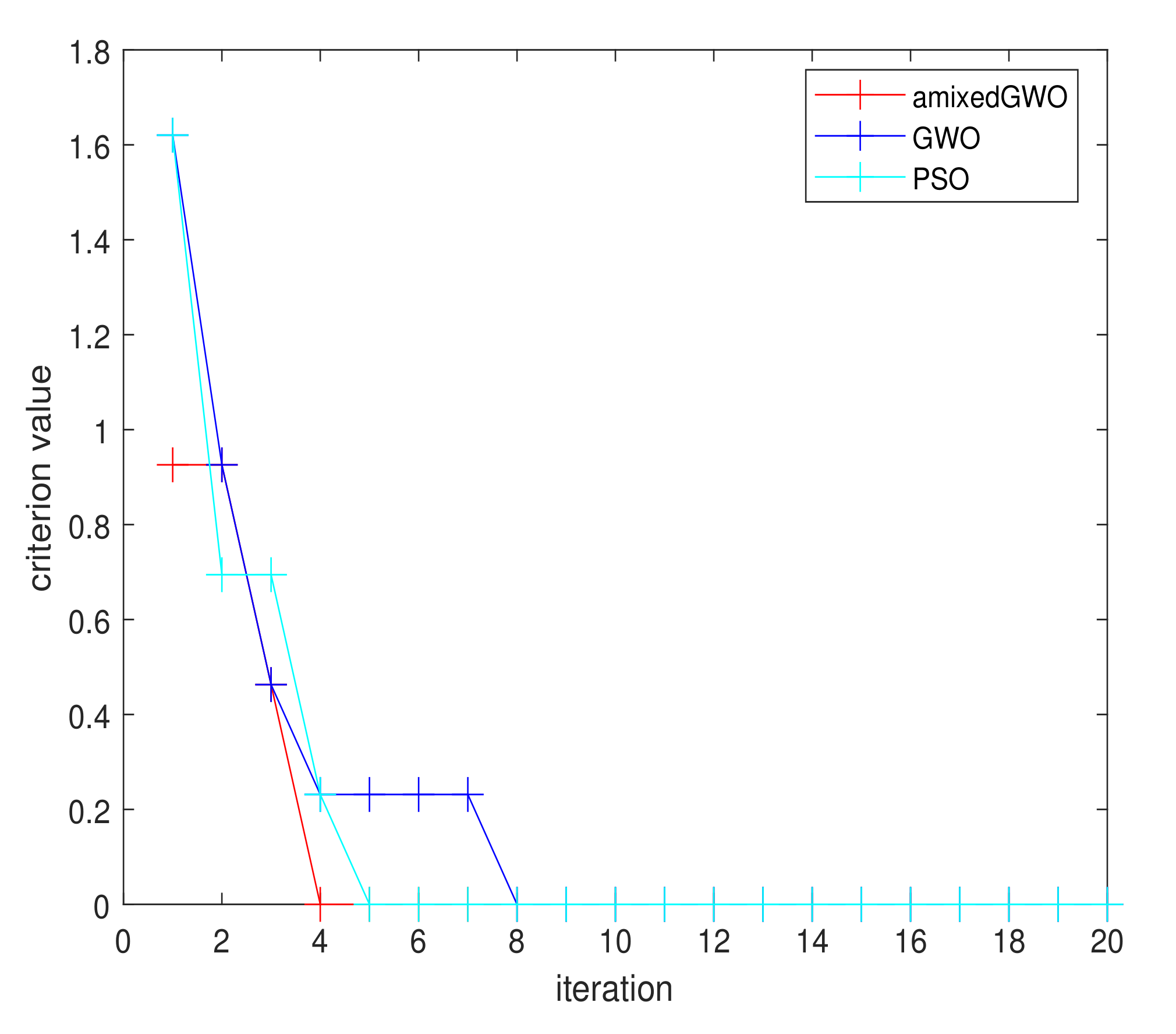
In Figure 19, we display the convergence curve obtained with amixedGWO, PSO and GWO. The curve reaches 0 at the 4th iteration when amixedGWO is used, at the 5th iteration when PSO is used, and at the 8th iteration when GWO is used. The best combination of parameters, provided as a solution by the amixedGWO algorithm, is

$${\left[\mathrm{V},94,0.8755,4,\mathrm{Z},\mathrm{polynomial},100,1000\right]}^T$$

(10)

the solution provided by PSO is as follows:

$${\left[\mathrm{V},96,0.7873,6,\mathrm{Z},\mathrm{polynomial},18.19,45.86\right]}^T$$

(11)

and the solution provided by GWO is as follows:

$${\left[\mathrm{H},96,0.33594,6,\mathbf{comb},\mathrm{polynomial},39.04,53.46\right]}^T$$

(12)

In the three cases, we reach $FRR=0.0\%$. What we notice from Equations (10)–(12) is that the parameters are different from one solution to another, except the kernel. This means that if the image processing parameters are correctly chosen, the user may decide to use any polarization and frequency value, depending on his constraints.

The images in Figure 12 were obtained with the threshold value 0.875 of the optimal vector presented in Equation (10). The confusion matrix obtained through the cross-validation process with SVM, and with these optimal parameter values, is displayed in

Table 5. Confusion matrix of licit/non licit object classification.

Objects	Guns	Knives	Licit
Guns	144	0	0
Knives	0	144	0
Licit	0	0	144

.

All other parameters being set to the values in Equation (10), we ran the classification algorithm with all possible values for the polarization and the kernel. The subsequent results in terms of number of misclassified images are presented in

Table 6. Number of misclassified images in various conditions, for a set of 432 images in total.

	Polarization	‘H + V’	‘H’	‘V’
Kernel
linear		9	1	2
rbf		4	3	4
polynomial		2	3	0

.

From Table 6, we notice that, once the kernel is correctly chosen, the number of missclassified images is low whatever the polarization. A nonlinear kernel such as polynomial or rbf yields interesting results. In

Table 7. Number of misclassified images in various conditions, for a set of 432 images in total.

	Polarization	‘H + V’	‘H’	‘V’
(Threshold, Factor)
(0.4, sd)		32	25	18
(0.6, Z)		3	0	8
(0.8, comb)		3	1	3

, the same experiment was performed, with all possible values for the type of feature, three different values for the threshold parameter, and once again all polarization values.

From Table 6 and Table 7, we notice that, if the user really wants to reach an FRR value of 0 %, it is necessary to run the amixedGWO to select the adequate combination of polarization and kernel for a given frequency value.

The values presented in both Table 6 and Table 7 show that it is possible to avoid the generation of both ‘$\mathrm{H}$’ and ‘$\mathrm{V}$’ images if the image processing parameters are optimized, which yields a division by two of the time dedicated to the acquisition.

As a balance from this subsubsection: from Equations (10) and (12), we notice that three different sets of parameters may yield an $FRR$ value equal to 0, with a polarization value which is not ‘$\mathrm{H}+\mathrm{V}$’. This was confirmed from Table 6 and Table 7, where low- or even zero-valued $FRR$ figures were obtained with appropriate combinations of parameter values. We now present results obtained with these three optimized systems, on a ‘test’ database of images which have never been seen by the classifiers.

3.2.2. Test Phase with the Trained Classifiers Obtained with amixedGWO, PSO, and GWO

The optimal sets of parameters obtained during the cross-validation and with three comparative optimization methods are presented in Equations (10)–(12). They correspond to three different configurations of our system, provided by amixedGWO, PSO, and GWO respectively. Each configuration yields a cross-validation FRR equal to 0, but we have to check the abilities of the system with images which have never been seen during cross-validation, with a so-called ‘test database’. In the cross-validation database, 130 to 131 images were used for learning, and 14 to 15 images for validation. For testing, as usual practice, we use approximately the same number as for validation, namely 18 for each of the three classes.

In order to build the test database we proceed as follows: only bootstrap images are used, with rotation, scaling and translation parameters which are different from those used in Section 2.4, to ensure that no image of the test database was present in the cross-validation database. To create these bootstrap images, two original acquisitions were used. We perform experiments with a suposedly increasing level of difficulty. We remind that the field of view for a given set of images is covered by the green points as in Figure 2. To create the test database, we use original acquisitions which are either inside or outside the field of view (FOV) used at the cross-validation stage. Here is listed the way we selected the two original acquisitions depending on the experiment:

• Experiment 1: inside the FOV considered in cross-validation and close to the vertical;
• Experiment 2: inside the FOV considered in cross-validation and far from the vertical;
• Experiment 3: outside the FOV considered in cross-validation.

In

Table 8. Number of missclassified images out of 54 images for various system configurations and testing conditions.

	Learning Conditions	Amixed GWO Equation (10)	PSO Equation (11)	GWO Equation (12)
Experiment
1		2	4	0
2		0	0	0
3		0	0	2

we provide the number of misclassified images for these experiments.

Table 8 shows firstly that the numbers of misclassifed images are rather low, which means that the classifiers are robust to changes between cross-validation and test database. We notice that, in experiment 3, that is, in the most realistic and difficult case, amixedGWO yields a perfect result with no misclassified image. It is also the case for PSO, which yields however a worse result in experiment 1, with a higher computational load in parameter estimation (as mentionned in Section 3.2.1).

Further in the paper, we consider cases where the proposed optimization strategy faces image databases which are harsher to exploit, and yield an FRR value for cross-validation which is larger than 0.

3.2.3. Additional Experiments and Limitations of the Proposed Method

In this subsection, we aim at varying the experimental conditions compared to Section 3.2.1. We investigate the behavior of the amixedGWO in the case where we change the radar image cross-validation database. Unless specified, no test phase is performed because the FRR value obtained in these cases for cross-validation is larger than 0.

Influence of the Aquisition Angle

In the results presented in Section 3.2.1, 16 images from the original set of acquisitions are used, to get a final number of 144 images for each class. Let us now consider cases where the acquisition angle with respect to the scene may be more elevated: in this case a sequence of acquisitions retrieves more images, from angular positions which are farther from the vertical axis. We use $N_1=N_2=N_3=36$ images for each class ($N=108$ in total) from the original acquisitions, and we do not perform bootstrap. All the 108 images obtained after segmentation of the acquisitions are available as png images at the following links: [42] (rar format), and [43] (zip format).

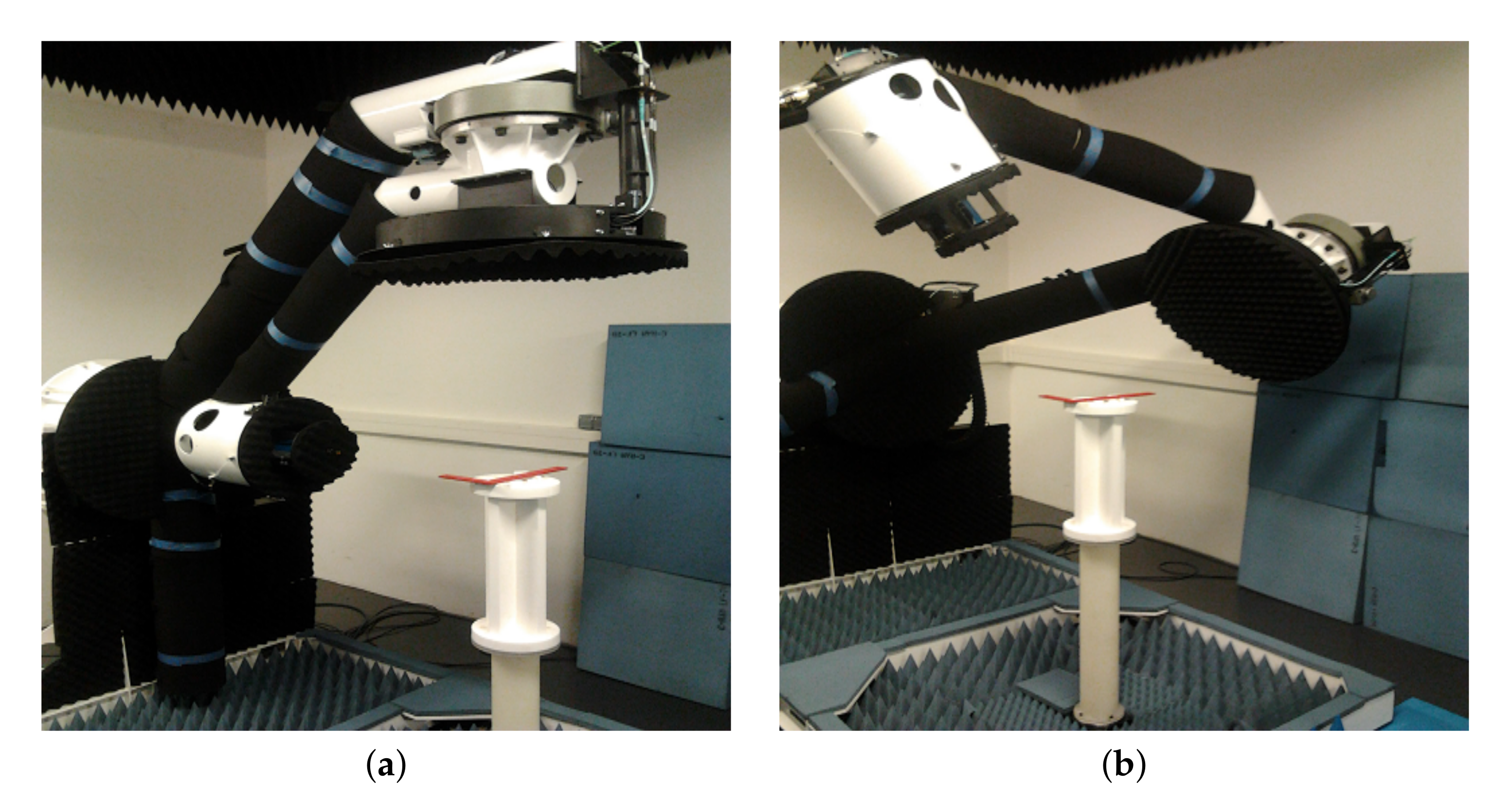
Let’s remind that, in Section 2, in Figure 2, we illustrate two cases, where the sensor remains close to the vertical axis (Figure 2a) or goes far from the vertical axis (Figure 2b). In the last case, we afford more acquisitions but they may be of a lower quality. Additionnally, we show in Figure 20 the sensor when it acquires an image rather close to the vertical axis (Figure 20a) or far from the vertical axis (Figure 20b).

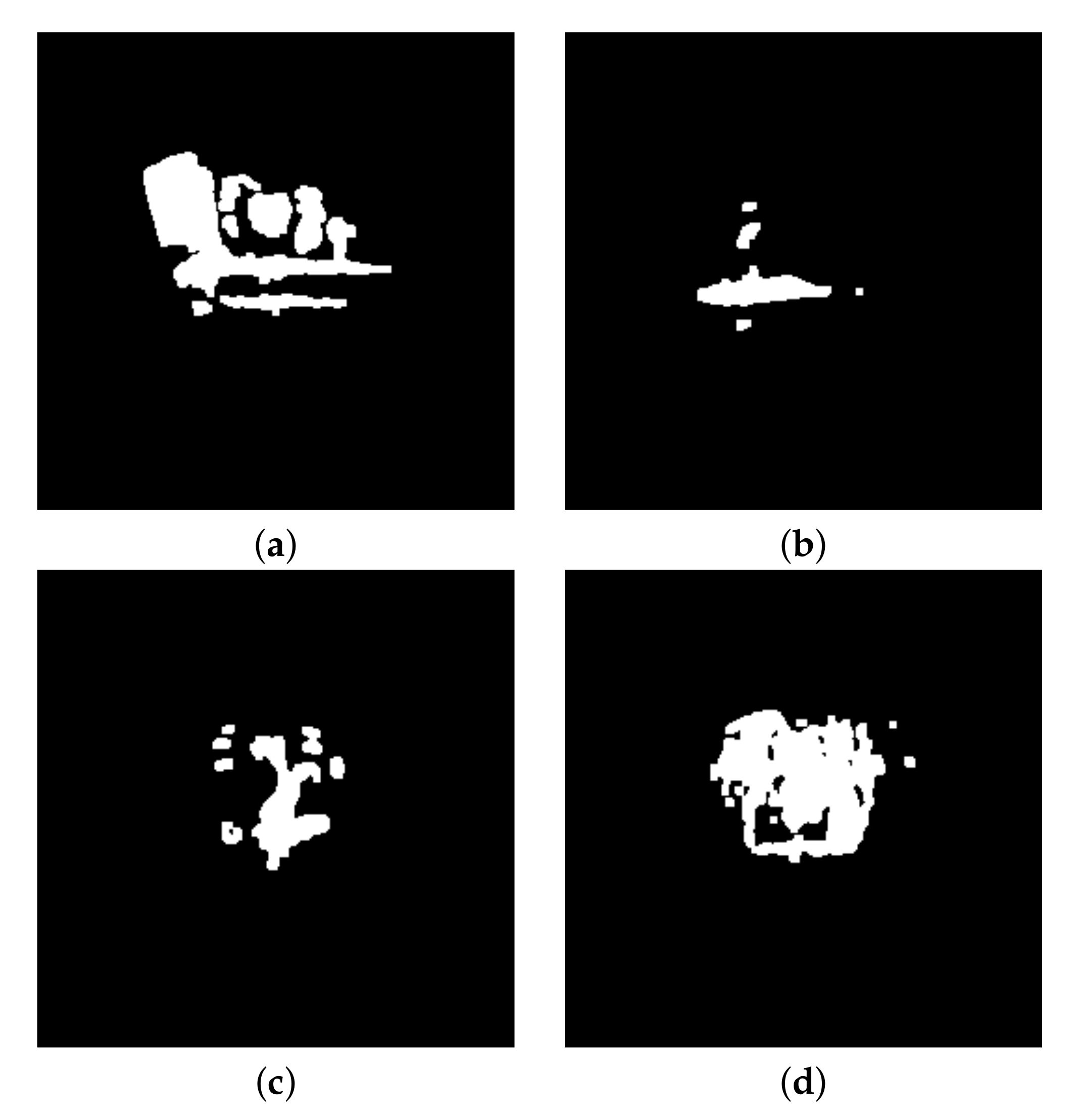
Now in Figure 21 we exemplify the resulting images, acquired far from the vertical axis, and obtained after segmentation: Figure 21a shows a gun, Figure 21b shows a knife, Figure 21c a set of keys, and Figure 21d a smartphone.

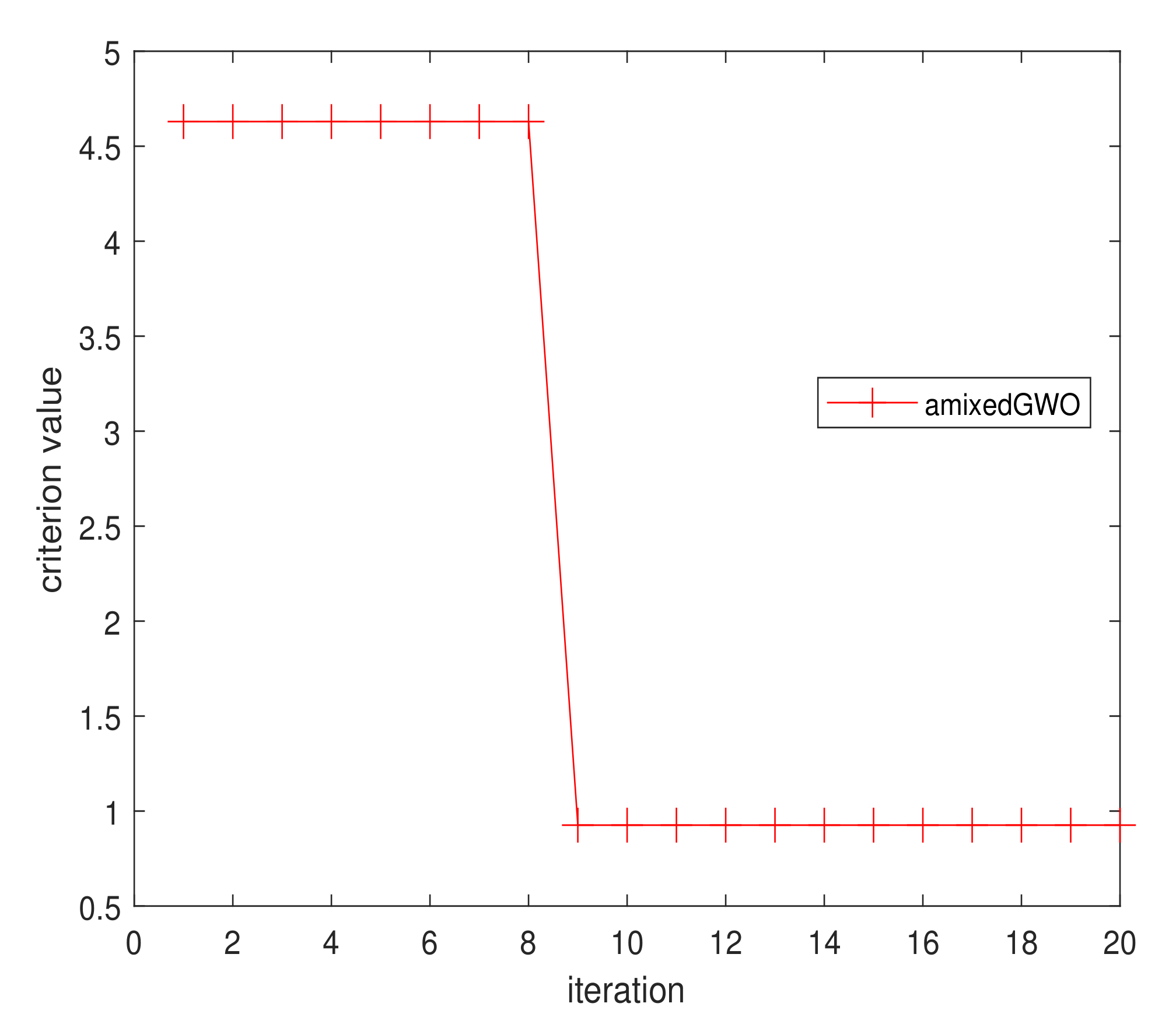
In this case, compared to Section 3.2.1, we select more images acquired far from the vertical axis, and part of the object is missing (see the gun in Figure 21a). When we run the amixedGWO to estimate anew the optimal parameters we get the convergence curve in Figure 22.

The optimal parameters are as follows:

$${\left[\mathrm{H},94,0.57568,4,\mathbf{comb},\mathrm{polynomial},10,10\right]}^T$$

(13)

With the set of parameters in Equation (13), the FRR is $0.93\%$. A careful look at the confusion matrix displayed in

Table 9. Confusion matrix of lethal/licit object classification.

Objects	Guns	Knives	Licit
Guns	36	0	0
Knives	0	36	0
Licit	0	1	35

permits to interpret this result.

Table 9 shows that 1 object is misclassified, out of 108: a licit object is classified as a lethal object. So the algorithm breaks down. In these conditions, the FRR is not 0, but this is the less dangerous case: in this situation, a person in charge checks the possibly dangerous individual, and lets him go.

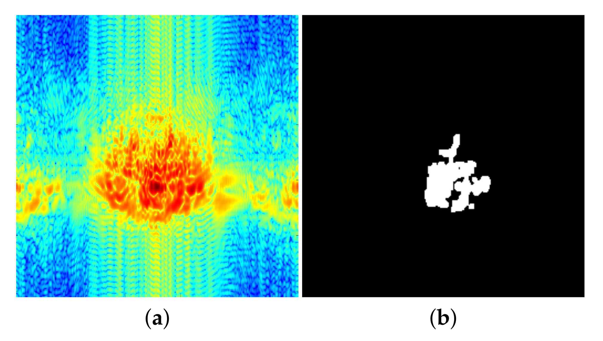
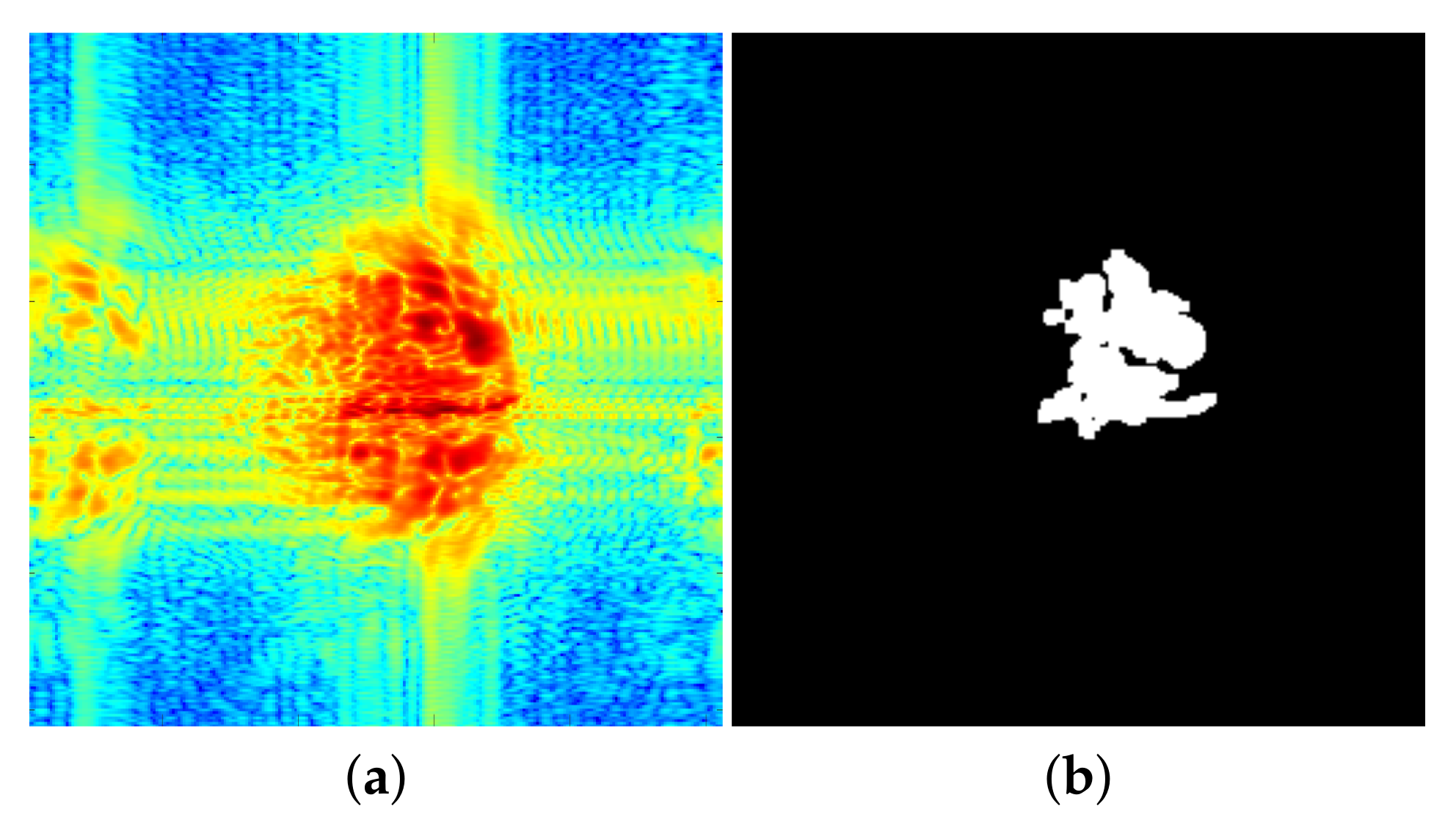
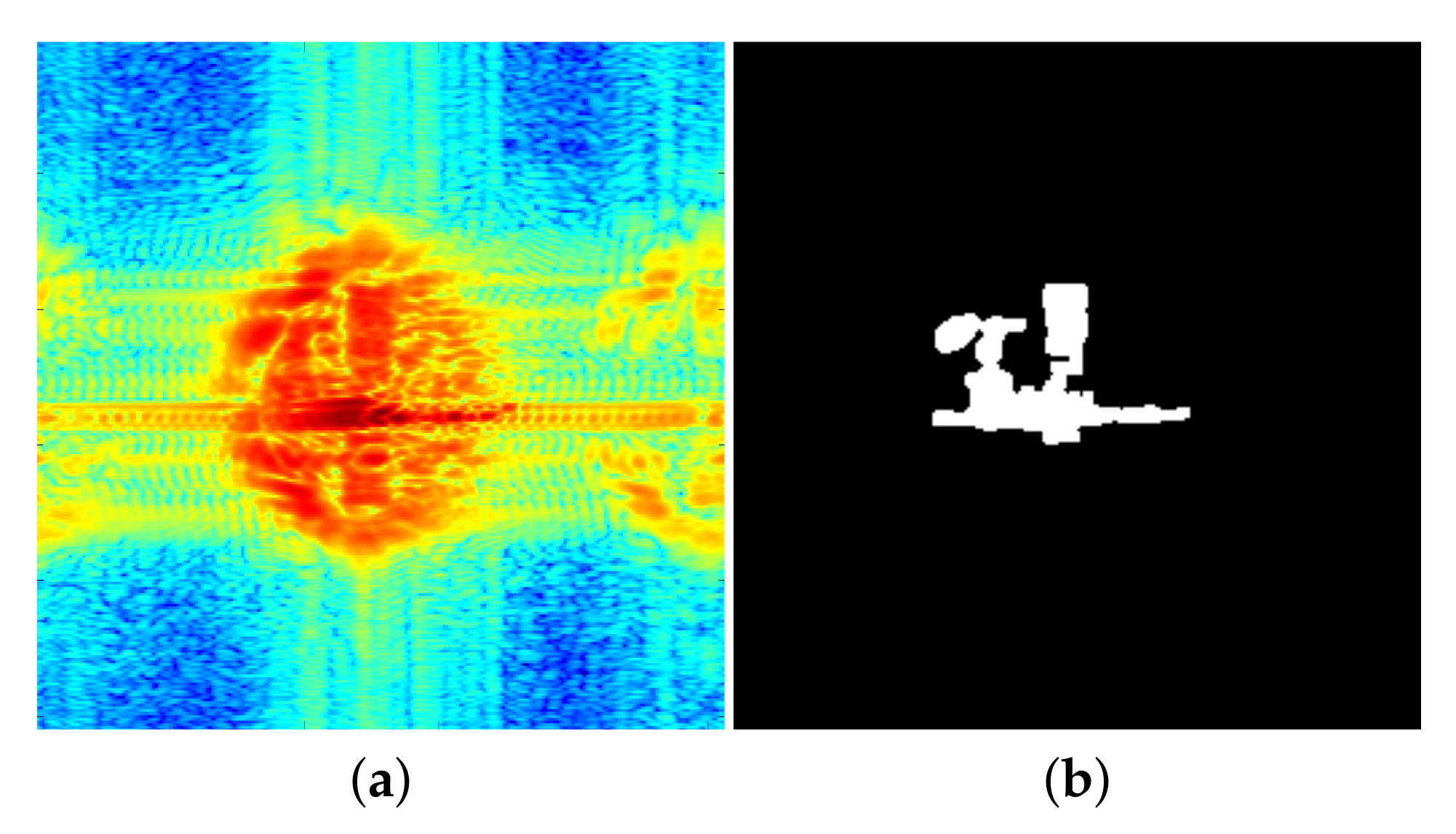
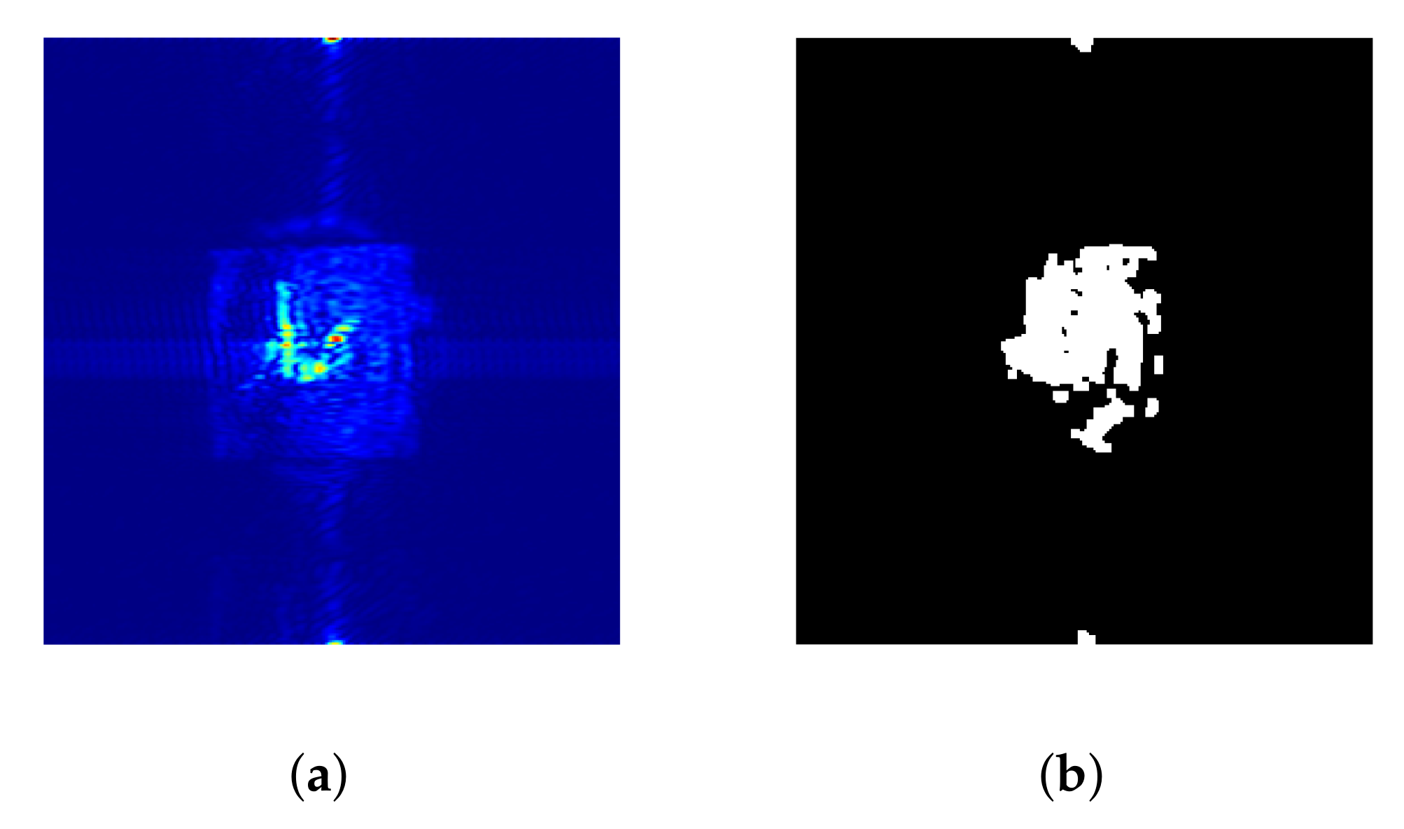
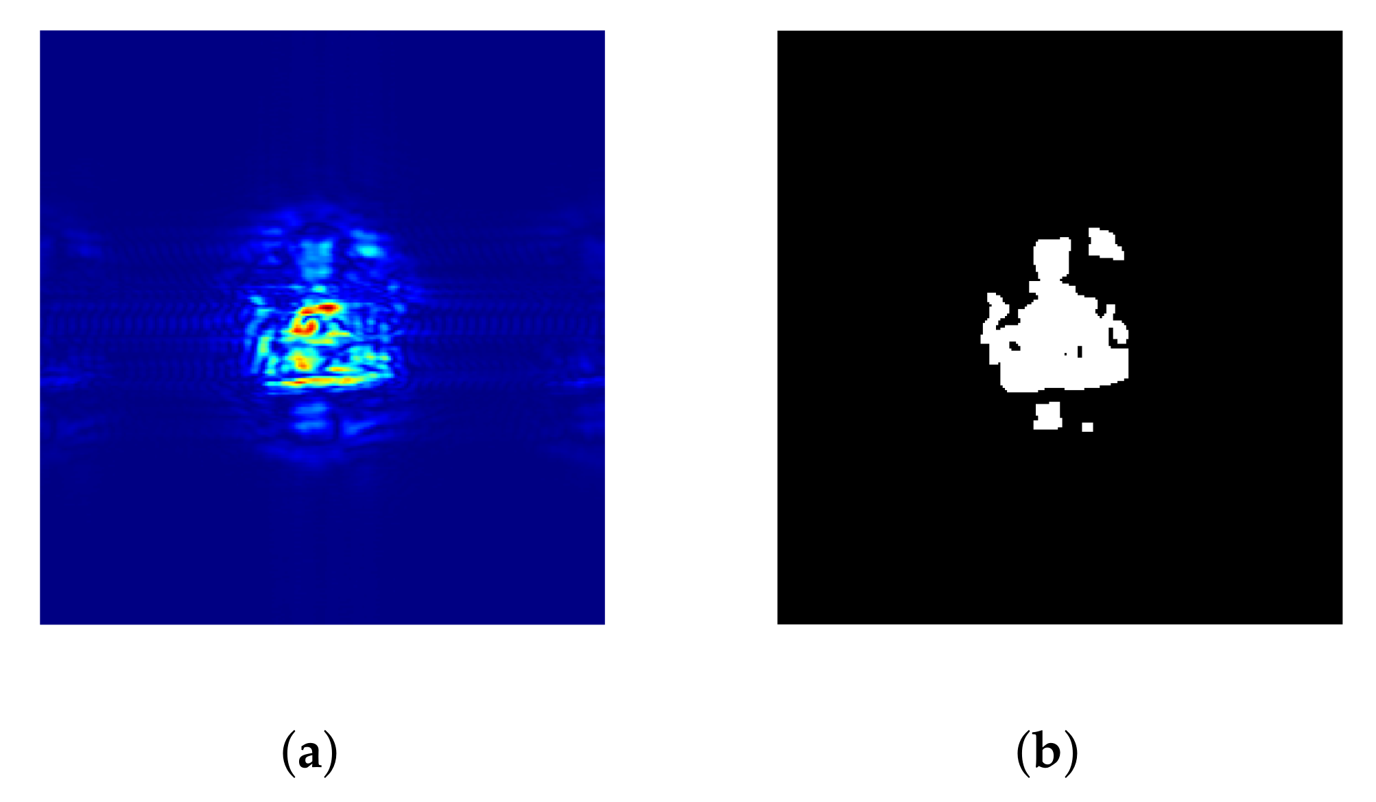
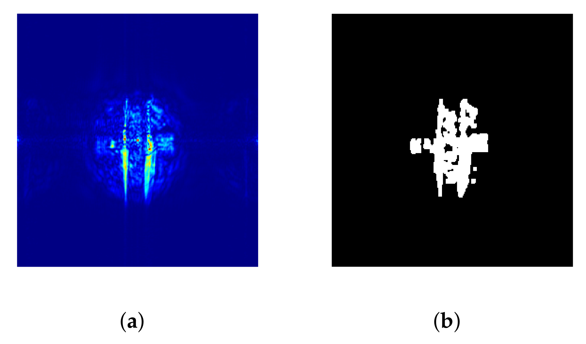
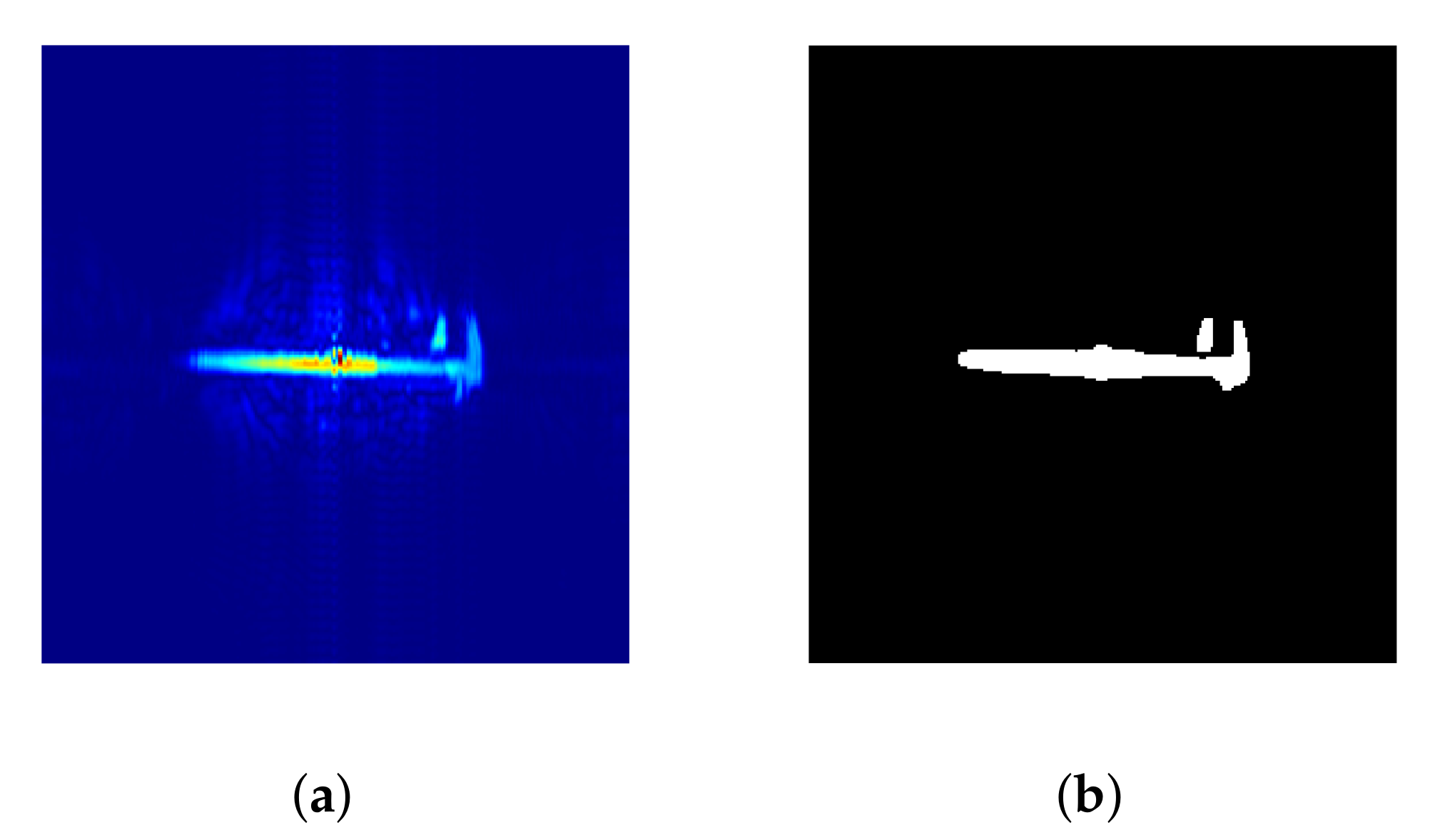
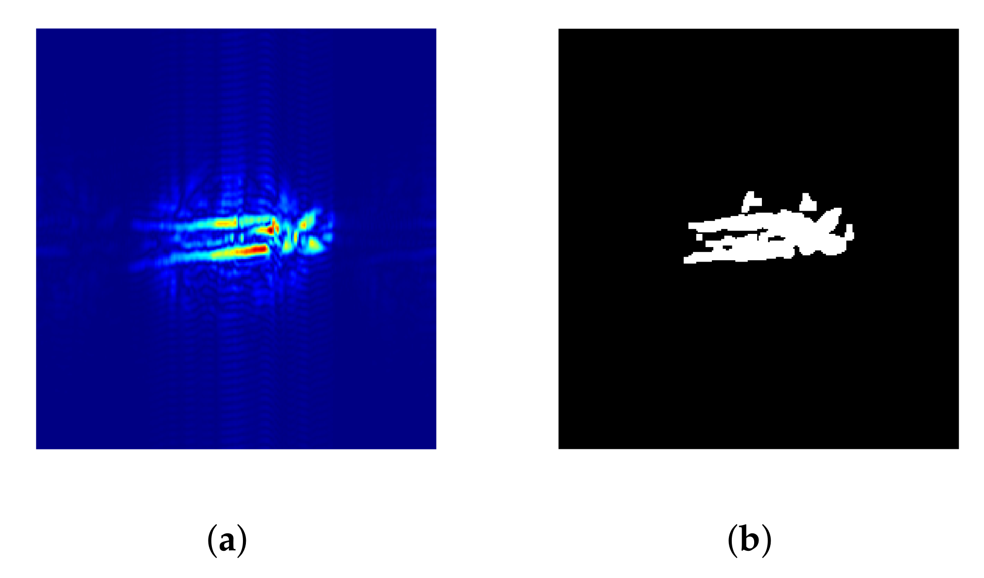
In Figure 23 we display the misclassified image (a set of keys): original scan in Figure 23a and segmented image in Figure 23b. In Figure 24 we display an example of image obtained from a knife. Looking at those two images, we notice that Figure 24b looks like a symmetric version of Figure 23b along a horizontal axis. Therefore, we can understand that the classification algorithm makes a confusion between these two images, and that a set of keys may be considered as a knife.

We remind that the feature selected by the amixedGWO in this case is ‘comb’. It is a vector of 491 components. If an image is misclassified, it means that it is similar to some images of the predicted class. This similarity can be measured through the scaled distance between the feature computed from the misclassified image and the feature computed from any image belonging to the predicted class. Similar images yield a small distance. The scaled distance between the features computed from Figure 23b and Figure 24b is equal to 50.3. In comparison, the scaled distance between the features computed from two other images of keys and knife (both correctly classified) is equal to 93.3. The first figure (50.3) is about two times smaller than the second one (93.3), which confirms the impression of similarity between the misclassifed image of keys and the comparative image of knife.

As in this case the variability in the set of images may be more elevated than in the case where bootstrap is applied, we wanted to check the reproducibility of the classification results obtained with the optimal parameters selected by the amixedGWO and presented in Equation (13). With this set of parameters, we ran 1000 times the classification algorithm (still on the cross-validation database). In

Table 10. Statistical study: number of misclassifications vs. counts, for 1000 counts in total.

Number of Misclassified Images	0	1	2	3	4	5	6	7	8	9
Counts	0	392	0	385	96	79	27	18	0	3

, we display the number of counts for each number of misclassifications.

For example, in Table 10, the column 2 indicates the values 1 and 392. This means that, among the 1000 trials, 392 trials yielded an experiment where only 1 image was misclassified. The case where no image is misclassified never occurs. Actually the image displayed in Figure 23 is never correctly classified. When a single image is misclassified, it is always the image displayed in Figure 23. This is the most current case, followed by the case where 3 images are misclassified.

Optimal Parameters for a Novel Frequency Value

In addition to the acquisitions at 94 and 96 GHz, we performed acquisitions at the frequency 92 GHz. We performed another experiment of cross-validation. As in Section 2.4, the number of scans is 16 and the total number of images is 144, for each class. However, when the knife is considered for acquisition, the angular step between each acquisition of knife is multiplied by 2. That is, the sensor goes farther from the vertical axis. For this specific frequency, we ran the amixedGWO. The solution it provides is as follows:

$${\left[\mathrm{H}+\mathrm{V},92,0.724,4,\mathbf{sd},\mathrm{polynomial},1,100\right]}^T$$

(14)

In Equation (14), the second parameter is of course 92 GHz because only this frequency is considered for this experiment.

In these conditions, we reach $FRR=0.23\%$. The confusion matrix obtained at the last iteration of the amixedGWO is as follows:

Table 11. Confusion matrix of licit/non licit object classification, for the best parameters at frequency 92 GHz.

Objects	Guns	Knives	Licit
Guns	144	0	0
Knives	0	143	1
Licit	0	0	144

shows that only one image is misclassified: a knife is considered as licit. We notice that for this frequency, compared to the solution provided in Equation (10), 3 parameters are similar or equal: the type of kernel (polynomial), the threshold parameter (0.72 instead of 0.87), and the size of the structuring element (4). We could also notice, during an additional experiment, that if the polarization is changed from ‘$\mathrm{H}+\mathrm{V}$’ to ‘$\mathrm{V}$’ as in Equation (10) or to H, only one or two additional images are missclassified. For instance, a licit object is considered as a knife. This may vary because of the random aspect of k-fold. As a consequence, and because a zero-valued $FRR$ is not available in this case, we could advise the end-user to use either ‘$\mathrm{H}$’ or ‘$\mathrm{V}$’ polarizations instead of ‘$\mathrm{H}+\mathrm{V}$’, to reduce the computational load.

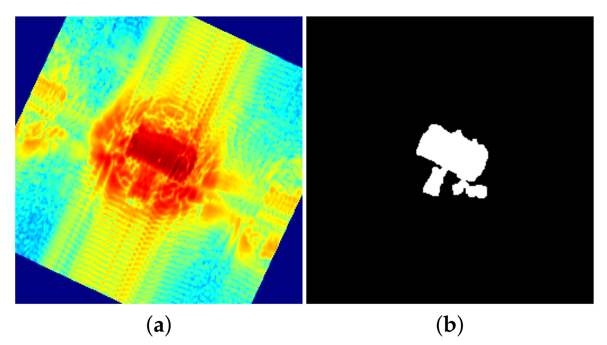
We could also notice that the non-zero $FRR$ value is not due to the change of frequency: running the amixedGWO in the same conditions as in Section 2.4, and with the same angular step yields an optimal $FRR$ value equal to 0. The fact that our amixedGWO does not reach a zero-valued FRR is really due to the wide span of acquisition angles, and can be explained while looking carefully at the misclassified image. We display in Figure 25 the scan and segmented image of knife which is classified as a licit object, and in Figure 26 an example of image obtained from a smartphone (scan and segmented image). At the first glance we notice that this image results from scaling and rotation applied in the bootstrap algorithm.

We notice that the image of the knife does not really look like an actual knife, contrary to the case of the RGB mmW images (see Figure 25b). Indeed the threshold value is such that pixels belonging to the rohacell tower below the object remain in the segmented image. This means that the contrast between the knife and the rohacell tower is lower than in the case of the gun for instance. There is also an overall squared shape which may remind a smartphone (though a hole is present inside). We can see that the rohacell tower is also visible in the image of smartphone (see Figure 26b). Hence, and remembering that the features extracted from the segmented images are invariant to rotation, translation, and scaling, we understand easily that the classification algorithm may missclassify this image of knife, whatever the image processing and machine learning parameters.

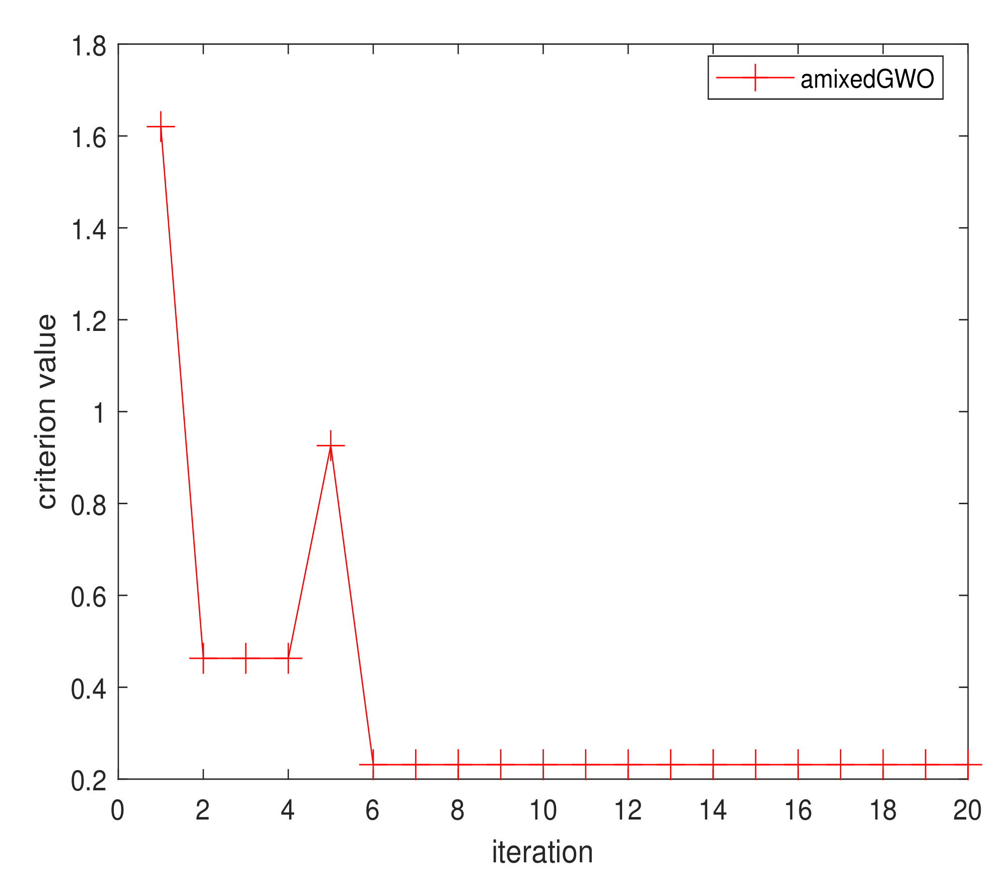
This experiment is also interesting in the sense that it illustrates the random aspect of the function $FRR\left(\mathbf{x}\right)$ mentionned in the first paragraph of Section 2.4 and exemplified in Table 10 above. In this experiment it induces an effect on the convergence curve. The convergence curve for this experiment, displayed in Figure 27, is not always decreasing. At iterations 2 to 4, the best score is always 0.46. We can notice that, at iteration 5, no search agent yielded 0.46 as a criterion value, even the agent which had been selected as the best one over all iterations up to the previous iteration. This means that for this agent, whose position has not changed, the score has changed, because the objective function $FRR\left(\mathbf{x}\right)$ itself has changed. After iteration 5, the convergence curve keeps decreasing in a usual manner: starting from iteration 6, a novel global minimum has been found at score 0.23, which remains the same until the last iteration.

In other words, the position of the global minimum of the objective function may be moving across iterations for this kind of application. We should consider the development of an improved version of the amixedGWO, which, in any manner, could better handle such a situation of moving minimum.

New Objects in the Database

In a practical use of the proposed approach, other licit objects than keys and smartphones may be encountered, and other metallic objects than the fake gun we have used may be considered as dangerous.

So we exemplify the algorithm with other objects: a new set of keys, a billfold, which has the same overall shape as a smartphone, a caliper, pliers, a bracket, and two knives. For each object we use 1 original acquisition at the vertical with respect to the scene, and 8 images obtained by bootstrap.

We perform a test phase, with the classifier obtained by amixedGWO (refer to Equation (10)): for each object an illustration of the acquisition and corresponding segmentation is provided in Figure 28, Figure 29, Figure 30, Figure 31, Figure 32 and Figure 33.

Firstly, we performed an experiment involving only the testing phase.

Table 12. Confusion matrix for additional objects; test phase only; 9 images among which 8 obtained by bootstrap.

	Predicted Class	Gun	Knife	Licit
Tested Objects
new set of keys		0	4	5
billfold		0	0	9
two knives		0	3	6
caliper		9	0	0
pliers		1	8	0
bracket		7	2	0

shows the obtained confusion matrix.

The images of caliper, pliers, and bracket are classified as ‘gun’ or ‘knife’. Considering the shape of these objects in the segmented image (see Figure 31, Figure 32 and Figure 33) we could easily argue that such an object can be considered as dangerous by the end-user of the system. In a practical case, the person in charge will stop the corresponding person for further investigation.

Secondly, we trained anew the classifier, with the parameters in Equation (10), but with additional objects in class 3: we added two acquisitions of caliper. For each class, we used 4 original acquisitions, and 32 additional images obtained by bootstrap. In the cross-validation experiment, only 1 image out of 108 was misclassified: a caliper was considered as a gun. We performed a test phase in the same conditions as in Table 12.

Table 13. Confusion matrix for additional objects; cross-validation and test phase; 9 images among which 8 obtained by bootstrap.

	Predicted Class	Gun	Knife	Licit
Tested Objects
new set of keys		0	0	9
billfold		0	0	9
two knives		0	7	2
caliper		0	0	9
pliers		0	9	0
bracket		4	0	5

shows the obtained confusion matrix. As expected, all the calipers are classified in class 3. It is also the case for 5 brackets out of 9. The algorithm has ‘learned’ correctly that a caliper is licit. Moreover, not only the calipers are correctly classified, but also all the images of the new set of keys, and some images of bracket: enriching one class with an appropriate object may improve the results obtained on several classes. In summary, when a new object is encountered by the end user, a possibility for him is to train anew the algorithm, deciding in what class he should place this new object.

3.3. Discussion

In this subsection our findings and their implications are discussed.

In a previous study by Migliaccio et al. [17], we have shown with some relevant examples that there exists a dependence of the visual aspect of binarized images on some acquisition parameters such as polarization and frequency. However a rigourous method allowing to choose the best value of acquisition parameters and threshold was missing in the literature, even in the works authored by people working on radar data and computational imaging like Zhu et al. [5], Gollub et al. [6], or Nanzer et al. [7].

Although various applications of bio-inspired optimization algorithms have been considered by Mirjalili et al. [18], Kiran et al. [19], Mirjalili et al. [20], and Martin et al. [21] for instance, we could check that such a joint tuning of parameters, based on experimental data, had never been considered. Also, to the best of our knowledge, no paper emphasizes the interest of using the smallest possible number of agents in a given application. This has turned out to be very important in the considered application, where the computational time dedicated to one run of the objective function is particularly elevated.

With our amixedGWO, we have proposed, for the first time in this paper, to estimate the best set of values for the parameters of the whole acquisition and processing chain. The proposed criterion to find an optimal set of values is the FRR.

Firstly, in Section 3.1, we have analyzed the behavior of all the comparative algorithms in simulations: in addition to our amixedGWO [21], we tested PSO proposed by Kennedy and and Eberhart [23,24], GWO proposed by Mirjalili et al. [18], CGSA from Mirjalili et al. [20], and TSA from Kiran et al. [19]. For this, we created a synthetic function which is a surrogate of our practical application, and for which the number of unknowns and the search spaces are the same. Our experiments have shown that the amixedGWO behaves well in terms of convergence when the number of search agents is small, at the expense however of an elevated computational load at a given iteration. In a few words, amixedGWO converges with a smaller number of iterations. Secondly, with the experiments performed on experimental radar data in Section 3.2, we have demonstrated the ability of the amixedGWO to reach a zero-valued FRR in a cross-validation phase, and also a zero-valued FRR in realistic conditions for the test phase. We could also find out that the behavior of our amixedGWO is of great interest for our application where, for each run of the objective function, the computational time is elevated.

From the results obtained, we can conclude that our methodology can help radar designers to set their system specifications jointly with image processing parameters. This was the major objective of the paper.

Of course there exist some limitations to this approach: we have shown in Section 3.2.3 that, despite the good performances of our approach in general and amixedGWO in particular, we are limited by the intrinsic nature of our system: the FRR obtained during cross-validation may not be zero-valued if the quality of the acquisition is not good enough, for instance if the sensor is far from the vertical to the scene; the intrinsic random nature of the k-fold process used in cross-validation causes variations in the results obtained by our optimizer: an optimal set of parameters may yield a zero-valued FRR once and a positive FRR value during another experiment. Nevertheless, even in conditions which are difficult for instance in terms of orientation of the scene with respect to the sensor, amixedGWO yields the best possible set of parameters with a computational time which outperforms comparative methods. It also behaves well if new objects are introduced in the test database. For instance metallic objects which could be misleading such as a metallic bracket are considered as dangerous and a person in charge can proceed with further investigations. The end-user can also can enrich the learning database with relevant objects.

4. Conclusions

The overall purpose of this work is the joint tuning of parameters which concern both the hardware and the software part of a radar system, in a security check application. The hardware includes a spherical 3D scanner acting as a CW radar, where the frequency and polarization can be selected by the user. The software includes a machine learning algorithm, namely error correcting output code combined with support vector machine. Some preliminary experiments have shown that the best software parameters may not be the same for different couples of values of the hardware parameters.

Thus, we propose to adapt a mixed version of the grey wolf optimizer, which is a computational technique meant for the minimization of a criterion. Our amixedGWO is a metaheuristic which is able to search optimal parameters for a given criterion in both discrete and continuous search spaces.

Some encouraging comparative results have been presented where the amixedGWO outperforms other metaheuristics while minimizing a surrogate of our application: a function with the same number of variables and the same properties for the search spaces. When applied to our security check issue on experimental data, we emphasized the conditions where the amixedGWO provides successfully the parameter values which yield a false recognition rate equal to 0 on cross-validation classification.It outperforms the original continuous GWO and PSO in terms of convergence. We could notice that, if the image processing parameters are correctly tuned, it is possible to use either ‘$\mathrm{H}$’, ‘$\mathrm{V}$’, or the combination of ‘$\mathrm{H}$’ and ‘$\mathrm{V}$’ polarizations. This enables the end-user to choose rather ‘$\mathrm{H}$’ or ‘$\mathrm{V}$’ polarizations, and thereby, to reduce the computational load dedicated to the acquisition.

During a test phase, we obtained interesting results with systems tuned by three comparative optimization methods yielding small numbers of misclassified images. Our amixedGWO yields a zero-valued $FRR$ on the test database in the most difficult and realistic case. In additional experiments, with images of lower quality, we have checked that the false recognition rate is not 0 in cross-validation. But we mostly encounter the less dangerous situation where a licit object is classified as a lethal one. This application also permitted to face the case of a convergence curve which is not monotonically decreasing, and to check the behavior of our amixedGWO in this situation.When new objects are encountered, they are correctly classified in a test phase if their shape is similar to objects which were present in the cross-validation base. Some licit objects are classified as lethal, but with good reasons. Otherwise, the new objects can be added in the cross-validation base, in the class which is considered as the most appropriate by the end-user.

As further works, there may still be issues to consider: it may be possible to reduce the time required by the acquisitions, and to optimize the error correcting codes to possibly handle situations with images of a lower quality. Also, an improved version of the amixedGWO, dedicated to the minimization of objective functions with moving minima, should be investigated.

References

1. Gentile, C. Application of Microwave Remote Sensing to Dynamic Testing of Stay-Cables. Remote Sens. 2009, 2, 36–51. [Google Scholar] [CrossRef] [Green Version]
2. Chai, S.S.; Walker, J.; Makarynskyy, O.; Kuhn, M.; Veenendaal, B.; West, G. Use of Soil Moisture Variability in Artificial Neural Network Retrieval of Soil Moisture. Remote Sens. 2009, 2, 166–190. [Google Scholar] [CrossRef] [Green Version]
3. Lv, X.; Ming, D.; Lu, T.; Zhou, K.; Wang, M.; Bao, H. A New Method for Region-Based Majority Voting CNNs for Very High Resolution Image Classification. Remote Sens. 2018, 10, 1946. [Google Scholar] [CrossRef] [Green Version]
4. Lin, W.; Li, Y. Parallel Regional Segmentation Method of High-Resolution Remote Sensing Image Based on Minimum Spanning Tree. Remote Sens. 2020, 12, 783. [Google Scholar] [CrossRef] [Green Version]
5. Zhu, R.; Richard, J.T.; Brady, D.J.; Marks, D.L.; Everitt, H.O. Compressive sensing and adaptive sampling applied to millimeter wave inverse synthetic aperture imaging. Opt. Express 2017, 25, 2270–2284. [Google Scholar] [CrossRef] [PubMed]
6. Gollub, J.; Yurduseven, O.; Trofatter, K.; Arnitz, D.; Imani, M.; Sleasman, T.; Boyarsky, M.; Rose, A.; Pedross-Engel, A.; Odabasi, H.; et al. Large metasurface aperture for millimeter wave computational imaging at the human-scale. Sci. Rep. 2017, 7, 42650. [Google Scholar] [CrossRef] [Green Version]
7. Nanzer, J.A. Microwave and Millimeter-Wave Remote Sensing for Security Applications; Artech House: Norwood, MA, USA, 2012. [Google Scholar]
8. Vakalis, S.; Gong, L.; He, Y.; Papapolymerou, J.; Nanzer, J.A. Experimental Demonstration and Calibration of a 16-Element Active Incoherent Millimeter-Wave Imaging Array. IEEE Trans. Microwave Theory Tech. 2020, 68, 3804–3813. [Google Scholar] [CrossRef]
9. Vakalis, S.; Nanzer, J.A. Analysis of Array Sparsity in Active Incoherent Microwave Imaging. IEEE Geosci. Remote Sens. Lett. 2020, 17, 57–61. [Google Scholar] [CrossRef]
10. Vakalis, S.; Gong, L.; Papapolymerou, J.; Nanzer, J.A. 40-GHz Active Interferometric Imaging with Noise Transmitters. In Proceedings of the 2019 16th European Radar Conference (EuRAD), Paris, France, 2–4 October 2019; pp. 273–276. [Google Scholar]
11. Yurduseven, O.; Smith, D.R.; Fromenteze, T. Computational Millimeter-wave Spotlight Imaging using Holographic Metasurface Antennas. In Proceedings of the 2018 IEEE International Symposium on Antennas and Propagation USNC/URSI National Radio Science Meeting, Boston, MA, USA, 8–13 July 2018; pp. 1461–1462. [Google Scholar]
12. Imani, M.F.; Gollub, J.N.; Yurduseven, O.; Diebold, A.V.; Boyarsky, M.; Fromenteze, T.; Pulido-Mancera, L.; Sleasman, T.; Smith, D.R. Review of Metasurface Antennas for Computational Microwave Imaging. IEEE Trans. Antennas Propag. 2020, 68, 1860–1875. [Google Scholar] [CrossRef] [Green Version]
13. Beasley, P.D.; Binns, G.; Hodges, R.D.; Badley, R.J. Tarsier/spl R/, a millimetre wave radar for airport runway debris detection. In Proceedings of the First European Radar Conference, Amsterdam, The Netherlands, 11–15 October 2004; pp. 261–264. [Google Scholar]
14. Zeitler, A.; Migliaccio, C.; Moynot, A.; Aliferis, I.; Brochier, L.; Dauvignac, J.Y.; Pichot, C. Amplitude and phase measurements of scattered fields for quantitative imaging in the W-band. IEEE Trans. Antennas Propag. 2013, 61, 3927–3931. [Google Scholar] [CrossRef]
15. Nsengiyumva, F.; Migliaccio, C.; Brochier, L.; Lanteri, J.; Dauvignac, J.Y.; Pichot, C. 90 GHz-3D Scattered Field Measurements for Investigation of Foreign Object Debris. IEEE Trans. Antennas Propag. 2019, 67, 6217–6222. [Google Scholar] [CrossRef]
16. Nsengiyumva, F.; Migliaccio, C.; Pichot, C. Millimeter-Wave Imaging for FOD Detection. In Air Traffic Management and Systems III; Springer: Singapore, 2019; pp. 247–264. [Google Scholar]
17. Migliaccio, C.; Brochier, L.; Lantéri, J.; Lauga, P.; Marot, J.; Cosson, B. MMW Imaging using polarimetric measurements. In Proceedings of the 2019 16th European Radar Conference (EuRAD), Paris, France, 2–4 October 2019; pp. 265–268. [Google Scholar]
18. Mirjalili, S.; Mirjalili, S.M.; Lewis, A. Grey Wolf Optimizer. Adv. Eng. Softw. 2014, 69, 46–61. [Google Scholar] [CrossRef] [Green Version]
19. Kiran, M.S. TSA: Tree-seed algorithm for continuous optimization. Expert Syst. Appl. 2015, 42, 6686–6698. [Google Scholar] [CrossRef]
20. Mirjalili, S.; Gandomi, A.H. Chaotic gravitational constants for the gravitational search algorithm. Appl. Soft Comput. 2017, 53, 407–419. [Google Scholar] [CrossRef]
21. Martin, B.; Marot, J.; Bourennane, S. Mixed grey wolf optimizer for the joint denoising and unmixing of multispectral images. Appl. Soft Comput. 2019, 74, 385–410. [Google Scholar] [CrossRef]
22. Holland, J.H. Genetic algorithms. Sci. Am. 1992, 267, 66–72. [Google Scholar] [CrossRef]
23. Kennedy, J.; Eberhart, R. Particle swarm optimization. In Proceedings of the IEEE International Conference on Neural Networks, Perth, WA, Australia, 27 November–1 December 1995; pp. 1942–1948. [Google Scholar]
24. Eberhart, R.C.; Kennedy, J. A new optimizer using particle swarm theory. In Proceedings of the Sixth International Symposium on Micro Machine and Human Science, Nagoya, Japan, 4–6 October 1995; Volume 1, pp. 39–43. [Google Scholar]
25. Lu, C.; Gao, L.; Li, X.; Xiao, S. A hybrid multi-objective grey wolf optimizer for dynamic scheduling in a real-world welding industry. Eng. Appl. Artif. Intell. 2017, 57, 61–79. [Google Scholar] [CrossRef]
26. Medjahed, S.; Saadi, T.A.; Benyettou, A.; Ouali, M. Gray Wolf Optimizer for hyperspectral band selection. Appl. Soft Comput. 2016, 40, 178–186. [Google Scholar] [CrossRef]
27. Martin, B.; Marot, J.; Bourennane, S. Improved Discrete Grey Wolf Optimizer. In Proceedings of the 2018 26th European IEEE Signal Processing Conference, Rome, Italy, 3–7 September 2018; pp. 499–503. [Google Scholar]
28. Otsu, N. A threshold selection method from gray-level histograms. IEEE Trans. Syst. Man Cybern. 1979, 9, 62–66. [Google Scholar] [CrossRef] [Green Version]
29. Sghaier, M.O.; Foucher, S.; Lepage, R. River extraction from high-resolution sar images combining a structural feature set and mathematical morphology. IEEE J. Sel. Top. Appl. Earth Obs. Remote Sens. 2016, 10, 1025–1038. [Google Scholar] [CrossRef]
30. Yan, G.; Yu, M.; Yu, Y.; Fan, L. Real-time vehicle detection using histograms of oriented gradients and AdaBoost classification. Opt.-Int. J. Light Electron. Opt. 2016, 127, 7941–7951. [Google Scholar] [CrossRef]
31. Dalal, N.; Triggs, B. Histograms of oriented gradients for human detection. In Proceedings of the 2005 IEEE Computer Society Conference on Computer Vision and Pattern Recognition, San Diego, CA, USA, 20–25 June 2005; Volume 1, pp. 886–893. [Google Scholar]
32. Slamani, M.A.; Ferris, D.D. Shape-descriptor-based detection of concealed weapons in millimeter-wave data. In Optical Pattern Recognition XII; International Society for Optics and Photonics, SPIE Digital Library: San Diego, CA, USA, 2001; Volume 4387, pp. 176–186. [Google Scholar]
33. Boughnim, N.; Marot, J.; Fossati, C.; Bourennane, S. Hand posture recognition using jointly optical flow and dimensionality reduction. EURASIP J. Adv. Signal Process. 2013, 2013, 1–22. [Google Scholar] [CrossRef] [Green Version]
34. Amari, S.i.; Wu, S. Improving support vector machine classifiers by modifying kernel functions. Neural Netw. 1999, 12, 783–789. [Google Scholar] [CrossRef]
35. Duan, K.; Keerthi, S.; Poo, A.N. Evaluation of simple performance measures for tuning SVM hyperparameters. Neurocomputing 2003, 51, 41–59. [Google Scholar] [CrossRef]
36. Lin, S.W.; Ying, K.C.; Chen, S.C.; Lee, Z.J. Particle swarm optimization for parameter determination and feature selection of support vector machines. Expert Syst. Appl. 2008, 35, 1817–1824. [Google Scholar] [CrossRef]
37. Dietterich, T.G.; Bakiri, G. Solving multiclass learning problems via error-correcting output codes. J. Artif. Intell. Res. 1994, 2, 263–286. [Google Scholar] [CrossRef] [Green Version]
38. Escalera, S.; Tax, D.M.J.; Pujol, O.; Radeva, P.; Duin, R.P.W. Subclass Problem-Dependent Design for Error-Correcting Output Codes. IEEE Trans. Pattern Anal. Mach. Intell. 2008, 30, 1041–1054. [Google Scholar] [CrossRef] [Green Version]
39. Anguita, D.; Ghio, A.; Ridella, S.; Sterpi, D. K-Fold Cross Validation for Error Rate Estimate in Support Vector Machines. In Proceedings of the 2009 International Conference on Data Mining, DMIN 2009, Las Vegas, NV, USA, 13–16 July 2009; Volume 1, pp. 291–297. [Google Scholar]
40. Windeatt, T.; Ghaderi, R. Coding and decoding strategies for multi-class learning problems. Inf. Fusion 2003, 4, 11–21. [Google Scholar] [CrossRef]
41. Cameron, A.C.; Gelbach, J.B.; Miller, D.L. Bootstrap-Based Improvements for Inference with Clustered Errors. Rev. Econ. Stat. 2008, 90, 414–427. [Google Scholar] [CrossRef]
42. Marot, J.; Migliaccio, C.; Lanteri, J.; Lauga, P.; Bourennane, S. Image Results Remote Sensing, Rar Archive. 2020. Available online: https://www.fresnel.fr/perso/marot/Documents/ResultsRemoteSensing/Segmentations_for_website.rar (accessed on 8 September 2020).
43. Marot, J.; Migliaccio, C.; Lanteri, J.; Lauga, P.; Bourennane, S. Image Results Remote Sensing, Zip Archive. 2020. Available online: https://www.fresnel.fr/perso/marot/Documents/ResultsRemoteSensing/Segmentations_for_website.zip (accessed on 8 September 2020).
44. Marot, J. Toolbox Meta Heuristics. A free Software under CeCILL-B Licence. 2020. Available online: https://www.fresnel.fr/perso/marot/Documents/ToolboxMetaHeuristicsRS.zip (accessed on 8 September 2020).
Figure 1. Radar data acquisition setup.
Remotesensing 12 03097 g001
Figure 2. Schematics of the acquisition principles: (a) small angle, (b) large angle.
Remotesensing 12 03097 g002
Figure 3. (a) Fake gun; (b) radar acquisition.
Remotesensing 12 03097 g003
Figure 4. (a) Knives; (b) radar acquisition.
Remotesensing 12 03097 g004
Figure 5. (a) Set of keys; (b) radar acquisition.
Remotesensing 12 03097 g005
Figure 6. (a) smartphone; (b) radar acquisition.
Remotesensing 12 03097 g006
Figure 7. Scan amplitudes of a concealed gun, ‘ H ’ polarization: (a) 94 GHz; (b) 96 GHz.
Remotesensing 12 03097 g007
Figure 8. Continuous GWO: displacement of an agent q towards the center of mass of the leaders.
Remotesensing 12 03097 g008
Figure 9. Discrete GWO: displacement of an agent q towards a leader, either α , β , or δ , selected at random.
Remotesensing 12 03097 g009
Figure 10. Illustration of the image processing chain on a concealed gun, ‘ H ’ polarization, 94 GHz: (a) grey level, (b) enhanced, (c) binarized, (d) mathematical morphology.
Remotesensing 12 03097 g010
Figure 11. Illustration of the image processing chain on a concealed gun, ‘ H ’ polarization, 96 GHz: (a) grey level, (b) enhanced, (c) binarized, (d) mathematical morphology.
Remotesensing 12 03097 g011
Figure 12. Segmentation of ‘ V ’ images, at frequency 94 GHz: (a) concealed gun, (b) knife, (c) keys, (d) smartphone.
Remotesensing 12 03097 g012
Figure 13. Segmentation of ‘ V ’ images, at frequency 94 GHz, with threshold parameter 0.87 and size 4 for the structuring element: (a) gun, (a’) concealed gun, (b) knife, (c) keys, (d) smartphone.
Remotesensing 12 03097 g013
Figure 14. Segmentation of ‘ H + V ’ images, at frequency 94 GHz, with threshold parameter 0.59 and size 2 for the structuring element: (a) concealed gun, (b) knife, (c) keys, (d) smartphone.
Remotesensing 12 03097 g014
Figure 15. Objective function: (a) 3D plot; (b) 2D plot.
Remotesensing 12 03097 g015
Figure 16. Arithmetic mean of the convergence curves for amixedGWO, PSO, GWO, TSA, CGSA.
Remotesensing 12 03097 g016
Figure 17. Geometric mean (semi-log scale) of the convergence curves for amixedGWO, PSO, GWO, TSA, CGSA.
Remotesensing 12 03097 g017
Figure 18. Box plot of the performances for all methods.
Remotesensing 12 03097 g018
Figure 19. Convergence curve for amixedGWO, PSO and GWO: 16 original acquisitions, 144 images in total.
Remotesensing 12 03097 g019
Figure 20. Photographs of the acquisition principles: (a) small angle, (b) large angle.
Remotesensing 12 03097 g020
Figure 21. Segmented acquisitions, large angle: (a) gun, (b) knife, (c) keys, (d) smartphone.
Remotesensing 12 03097 g021
Figure 22. Convergence curve for amixedGWO, 36 acquisitions.
Remotesensing 12 03097 g022
Figure 23. Misclassified image of a set of keys: (a) RGB mmW scan; (b) Segmented image.
Remotesensing 12 03097 g023
Figure 24. Example of image of knife: (a) RGB mmW scan; (b) Segmented image.
Remotesensing 12 03097 g024
Figure 25. Misclassified image of knife: (a) RGB mmW scan; (b) Segmented image.
Remotesensing 12 03097 g025
Figure 26. Example of image of a smartphone: (a) RGB mmW scan; (b) Segmented image.
Remotesensing 12 03097 g026
Figure 27. Convergence curve for amixedGWO, with fixed frequency 92 GHz.
Remotesensing 12 03097 g027
Figure 28. New set of keys: (a) Scan; (b) Segmented image.
Remotesensing 12 03097 g028
Figure 29. Billfold: (a) Scan; (b) Segmented image.
Remotesensing 12 03097 g029
Figure 30. Two knives: (a) Scan; (b) Segmented image.
Remotesensing 12 03097 g030
Figure 31. Caliper: (a) Scan; (b) Segmented image.
Remotesensing 12 03097 g031
Figure 32. Pliers: (a) Scan; (b) Segmented image.
Remotesensing 12 03097 g032
Figure 33. Bracket: (a) Scan; (b) Segmented image.
Remotesensing 12 03097 g033