Evaluation of Methods for Mapping the Snow Cover Area at High Spatio-Temporal Resolution with VENμS

Abstract

The VEN$\mathsf{\mu }$S mission launched in 2017 provides multispectral optical images of the land surface with a 2-day revisit time at 5 m resolution for over 100 selected sites. A few sites are subject to seasonal snow accumulation, which gives the opportunity to monitor the variations of the snow cover area at unprecedented spatial and temporal resolution. However, the 12 spectral bands of VEN$\mathsf{\mu }$S only cover the visible and near-infrared region of the spectra while existing snow detection algorithms typically make use of a shortwave infrared band to determine the presence of snow. Here, we evaluate two alternative snow detection algorithms. The first one is based on a normalized difference index between the near-infrared and the visible bands, and the second one is based on a machine learning approach using the Theia Sentinel-2 snow products as training data. Both approaches are tested using Sentinel-2 data (as surrogate of VEN$\mathsf{\mu }$S data) as well as actual VEN$\mathsf{\mu }$S in the Pyrenees and the High Atlas. The results confirm the possibility of retrieving snow cover without SWIR with a slight loss in performance. As expected, the results confirm that the machine learning method provides better results than the index-based approach (e.g., an RMSE equal to the learning method 1.35% and for the index-based method 10.80% in the High Atlas.). The improvement is more evident in the Pyrenees probably due to the presence of vegetation which complicates the spectral signature of the snow cover area in VEN$\mathsf{\mu }$S images.

1. Introduction

The snow cover area, i.e., the areal extent of snow-covered ground [1], is a key variable in the study of mountain ecosystems [2]. In mountainous regions, the snow cover is characterized by a high spatial variability, which reflects the combined influence of the terrain, land cover and weather variability [3,4]. Therefore, high-resolution information (i.e., below 100 m) on the snow cover area is important to understand the dynamics of mountain ecosystems. For example, an accurate description of the snow cover area was critical to explain the spatial heterogeneity of both taxonomic and functional diversity of plant communities in an alpine grassland [5]. High-resolution snow cover area is also useful in hydrology to reduce biases in the spatial distribution of the snow water equivalent [6,7] and may become an important tool for economic activities like land management or tourism. For all the aforementioned applications, it is also important to characterize the snow cover evolution with a high temporal resolution especially during the melt season when significant reduction of the snow cover occurs at a daily rate.

VEN$\mathsf{\mu }$S is a micro-satellite in Sun-synchronous circular orbit with a superspectral camera which provides images with 12 narrow spectral bands in the visible and near infrared region (VNIR) [8,9]. VEN$\mathsf{\mu }$S was launched on 2 August 2017. The first phase of VEN$\mathsf{\mu }$S mission (after the commissioning phase) is devoted to the science mission objectives. It started in January 2018 and is planned to last 2.5 years. During this phase, VEN$\mathsf{\mu }$S camera acquires images from the nominal orbit at 720 km altitude for 110 selected sites. In this configuration, the sensor swath is 27.5 km, the ground spatial resolution is 5.3 m at nadir and the revisit time is 2 days. No other sensor currently in orbit combines this kind of revisit rate, spatial resolution and spectral bands [10]. Some VEN$\mathsf{\mu }$S sites are located in mountainous areas with a significant seasonal snow cover in winter: DESIP2 (USA), DESIP3 (USA), SUDOUEST (France and Spain), NARYN (Kirghizstan), KHUMBU (Nepal and China). Hence, these sites offer the opportunity to track subtle variations of the snow cover area at unprecedented spatial and temporal resolution. Orthorectified top-of-atmosphere reflectances products (level-1C) are delivered by the French Theia land data center with a pixel size of 5 m. Theia also provides surface reflectance products (level-2A) at 10 m resolution, which were generated using state-of-the-art atmospheric correction and cloud masking algorithm [11,12]. Currently, there is no snow product based on VEN$\mathsf{\mu }$S images, which indicates the presence or absence of snow, like the Theia snow collection for Sentinel-2 [13]. Therefore, our objective is to define a method to classify the snow cover from VEN$\mathsf{\mu }$S level-2A products (surface reflectance and cloud mask). However, the 12 spectral bands of VEN$\mathsf{\mu }$S only cover the VNIR spectral region while existing snow detection algorithms typically make use of a shortwave infrared (SWIR) band to determine the presence of snow in Landsat, MODIS, ASTER or Sentinel-2 images [13,14,15,16]. Indeed, this band permits to easily distinguish between snow-covered and snow-free areas, because snow has a high reflectance at visible wavelengths and very low reflectance in the SWIR [17,18]. This specific property of the snow cover led to the definition of the Normalized Difference Snow Index by Dozier [14]:

$$\mathrm{NDSI}=\frac{{\rho }_{\mathrm{green}}-{\rho }_{\mathrm{SWIR}}}{{\rho }_{\mathrm{green}}+{\rho }_{\mathrm{SWIR}}},$$

(1)

where ${\rho }_{\mathrm{green}}$ (resp. ${\rho }_{\mathrm{SWIR}}$) is the surface reflectance in the green channel (resp. SWIR at 1.6 $\mathsf{\mu }$m).

A few previous studies focused on retrieving the snow cover area from VNIR optical remote sensing images (without SWIR band). This is typically the case of very-high resolution images acquired by satellites like WorldView, Pléiades or Formosat-2. Bühler et al. [19] used very high spatial resolution WorldView-2 images and normalized difference band ratios from the visible and near infrared bands to distinguish and map different snow surfaces near Davos in Switzerland. The results showed that an NIR band between 860 and 1040 nm enabled identification of snow cover and distinguishing of spatial variations in the snow surface type. Marchane et al. [20] derived the snow cover area from Formosat-2 images at 8 m resolution (with red, green and near-infrared bands) using a supervised classification. This method provided accurate results but the training samples were manually collected by the visual interpretation of the image. Another drawback of the supervised approach is that the classification model may not be transferable to other study areas.

Here we seek a robust and automatic method to retrieve the snow cover area in VEN$\mathsf{\mu }$S images, i.e., without the need for human intervention. We focus on pixel-based approaches as they are more scalable than object-oriented classification algorithms (rarely used to classify dense time series of high resolution image). First, we evaluate a standard thresholding approach based on an modified normalized difference snow index. Then, we propose a machine-learning method which combines the advantage of the supervised approach (accuracy) and unsupervised approach (genericity).

We evaluate the method using the Theia Sentinel-2 snow product derived with SWIR bands as a reference. It covers a similar spectral range as VEN$\mathsf{\mu }$S bands (band 7 and 8 of Sentinel-2 corresponds respectively to the bands 10 and 11 in VEN$\mathsf{\mu }$S,

Table 1. Summary of VEN$\mathsf{\mu }$S and Sentinel-2 spectral bands.

VEN$\mathsf{\mu }$S		Sentinel-2
Number	Wavelength Center (nm)	Number	Wavelength Center (nm)
1	423.9	-	-
2	446.9	1	443.0
3	491.9	2	490.0
4	555.0	3	560.0
5	619.7	-	-
6	619.5	-	-
7	662.2	4	665.0
8	702.0	5	705
9	741.1	6	740
10	782.2	7	783
11	861.1	8a	865
12	908.7	-	-

). The extended coverage of Sentinel-2 and the availability of Sentinel-2 snow products from Theia allows evaluating our method in various sites.

2. Data and Methods

2.1. Data

2.1.1. Sentinel-2 Level-2A Products

Sentinel-2 data were obtained from the Theia level-2A collection [13]. Level-2A (L2A) products provide surface reflectances and a cloud mask that were generated by MAJA [21]. The surface reflectance is adjusted to account for the effect of the terrain slope on the observed reflectance in the sun-sensor geometry [21], which is an important feature for snow detection in mountain regions. We used respectively 11 and 18 images for tiles T29RPQ and T31TCH. We only selected images with a very low cloud cover (

Table 2. Date of acquisition of Sentinel-2 images for the two sites (T29RPQ and T31TCH) and (VEN$\mathsf{\mu }$S).

Tile High Atlas (S2)		Tile Pyrenees (S2)		Tile Pyrenees (VEN$\mathsf{\mu }$S)
Dates	Tile	Date	Tile	Date	Tile
2 January 2018	T29RPQ	1 January 2018	T31TCH	31 January 2018	SUDOUE-5
12 January 2018	T29RPQ	31 January 2018	T31TCH	2 March 2018	SUDOUE-5
17 January 2018	T29RPQ	25 February 2018	T31TCH	21 April 2018	SUDOUE-5
22 January 2018	T29RPQ	2 March 2018	T31TCH	20 June 2018	SUDOUE-5
27 January 2018	T29RPQ	7 March 2018	T31TCH	6 January 2019	SUDOUE-5
1 February 2018	T29RPQ	1 April 2018	T31TCH	15 February 2019	SUDOUE-5
1 February 2018	T29RPQ	21 April 2018	T31TCH	—	—
11 February 2018	T29RPQ	11 May 2018	T31TCH	—	—
21 February 2018	T29RPQ	20 June 2018	T31TCH	—	—
3 March 2018	T29RPQ	17 November 2018	T31TCH	—	—
23 March 2018	T29RPQ	7 December 2018	T31TCH	—	—
27 April 2018	T29RPQ	17 December 2018	T31TCH	—	—
—	—	27 December 2018	T31TCH	—	—
—	—	1 January 2019	T31TCH	—	—
—	—	6 January 2019	T31TCH	—	—
—	—	11 January 2019	T31TCH	—	—
—	—	16 January 2019	T31TCH	—	—
—	—	15 February 2019	T31TCH	—	—

). These data are freely accessible from Theia website [22]. Each level-2A product contains a 110 × 110 km${}^2$ ortho-image in UTM/WGS84 projection.

2.1.2. Sentinel-2 Snow Products

Sentinel-2 snow products were obtained from the Theia “snow” collection [13]. These products provide the snow presence or absence at 20 m resolution from Sentinel-2 observations. Theia snow products are routinely generated from Theia L2A products and freely available at Theia. In Theia, the snow detection is made based on the NDSI and a digital elevation model. The reader can refer to [13] for the details on the snow detection algorithm and its evaluation.

2.1.3. VEN$\mathsf{\mu }$S Level-2A Products

VEN$\mathsf{\mu }$S level-2A products were also obtained from Theia. Level-2 products provide atmospheric corrected surface reflectances and is supplied with a cloud mask and shadows. VEN$\mathsf{\mu }$S L2A products are also generated by MAJA using a multi-temporal approach [11].

VEN$\mathsf{\mu }$S snow masks were resampled to the same UTM grid as Sentinel-2 at 20 m resolution using the nearest neighbor method to allow the computation of the confusion matrix between both datasets [23]. The size of the tile is: 32.27 × 73.24 km${}^2$.

2.2. Methods

2.2.1. Unsupervised Classification

This method is based on a normalized difference index similar to the NDSI (Section 1), but using bands 10 (782 nm) and 11 (861 nm) in VEN$\mathsf{\mu }$S images, which correspond to bands 7 (783 nm) and 8a (865 nm) in Sentinel-2 images (Table 1). This index is based on the fact that the snow reflectance is lower at wavelength 861 nm than 782 nm [17]. This index is referred to as NDSI${}_{\mu }$:

$${\mathrm{NDSI}}_{\mu }=\frac{{\rho }_{\mathrm{B}10}-{\rho }_{\mathrm{B}11}}{{\rho }_{\mathrm{B}11}+{\rho }_{\mathrm{B}10}},$$

(2)

Non-cloud pixels with NDSI${}_{\mu }>n_0$ and with reflectance in the red and blue bands respectively higher than 0.12 and 0.17 are marked as snow. Red and blue bands thresholds were chosen after a preliminary study which explored different band combinations and thresholds (CNES internal report Theia-NT-413-0483-CNES). The $n_0$ threshold was optimized for each region T29RPQ and T31TCH by testing 40 linearly spaced values between −0.20 and 0.20. In both cases the highest Heidle skill score (HSS) was obtained with $n_0=0.01$, therefore this value was selected. However, we noted a low sensitivity to this value since the HSS (Section 2.3) varied only by ±0.01 and the resulting snow cover area by less than 2%.

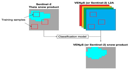
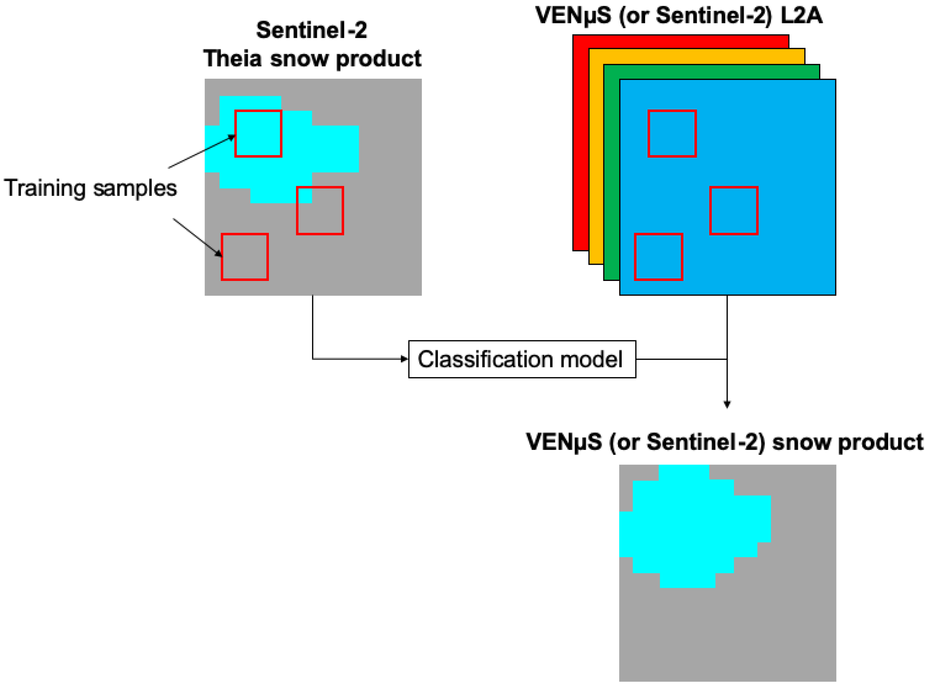
2.2.2. Supervised Classification

We developed a process to automatically obtain the training samples from the Sentinel-2 Theia snow products to train a supervised classifier (Figure 1). Theia snow products were considered as a reference dataset (or “ground truth”) since these products were generated using Sentinel-2 images including an SWIR band, which allow an accurate detection of the snow cover (Section 2.1.2).

First, we randomly extracted 20 subsets of 20 by 20 pixels from the Theia snow products. Connected regions of pixels with the same value (snow or no-snow) were converted to polygons with attribute snow or no-snow (using GDAL polygonize tool with 4 pixels connectedness). These polygons were used to train a support vector machine (SVM) algorithm [24] in the Orfeo Toolbox [25]. The training samples contained reflectances in bands green, red and NIR (i.e., B03, B04 and B08a for Sentinel-2 and B04, B07, B11 for VEN$\mathsf{\mu }$S). B02 (blue) was not considered due to the larger uncertainty in these wavelengths caused by atmospheric effects. This method is referred to below as the supervised classification (SC) method. The SVM algorithm was chosen based on preliminary tests with other classification methods available in the OTB library (random forest and KNN). The SVM training model will be applied for all images.

2.3. Evaluation Strategy

In a first stage, the two classification methods described in Section 2.2 were evaluated using Sentinel-2 images as input, and the corresponding Theia snow products as validation data. Hence, Sentinel-2 data were used as a surrogate for VEN$\mathsf{\mu }$S data. This approach aims to augment the evaluation dataset given that few synchronous Sentinel-2 and VEN$\mathsf{\mu }$S were available. However, we used only Sentinel-2 spectral bands which are also available from VEN$\mathsf{\mu }$S (green, red and NIR, more details below). The main advantage of this approach is the exact spatial and temporal collocation of the result with the validation data (Theia is also derived from Sentinel-2). It also allowed an evaluation of the algorithm in Morocco where there is currently no VEN$\mathsf{\mu }$S acquisitions, but the Theia data are available. This evaluation in Morocco was motivated to evaluate the transposability of the results to semi-arid mountain regions like western Colorado, where there are two VEN$\mathsf{\mu }$S sites.

The evaluation was done at two contrasted sites (Figure 2). The first site is located in the High Atlas mountains in Morocco (Sentinel-2 tile T29RPQ). This tile contains many peaks above 3000 m asl including the highest peak of the High Atlas range, Djebel Toubkal (4167 m). In this site, the snow usually covers the areas above 2500 m asl throughout the winter season. At these elevations, the vegetation is very scarce due to the arid and cold climate [20]. The second site is located in the Pyrenees mountains (Sentinel-2 tile T31TCH), where the vegetation is more developed even in the snow dominated areas, i.e., roughly above 1600 m asl [26]. The histograms of the slopes and aspect from the SRTM digital elevation model are provided in the Supplementary Materials.

In a second stage, we evaluate the method using actual VEN$\mathsf{\mu }$S data in the Pyrenees. We selected VEN$\mathsf{\mu }$S images that were acquired on the same day or with a time lag of 1 day as a Sentinel-2 acquisition. There are six dates that are given in Table 2. This allowed us to compare the VEN$\mathsf{\mu }$S snow products to Sentinel-2 Theia snow products. This comparison was done in the intersection area between Sentinel-2 tile T31TCH and VEN$\mathsf{\mu }$S tile SUDOUE-5. This subset area is shown in Figure 2.

2.4. Evaluation Criteria

To evaluate the different products of classifications, we used Theia snow products as the truth. The evaluation was carried out by comparing the evolution of the snow cover area (SCA) at the tile scale with the mean error (ME) and root mean square error (RMSE). In addition, we performed a pixel-wise evaluation using the Heidle skill score, which is a statistical index derived from the confusion matrix (HSS) [27]:

$$\mathrm{HSS}=\frac{2(TP\times TN-FP\times FN)}{(TP+FP)\times (FP+TN)+(TP+FN)(FN+TN)}$$

(3)

where $TP$, $TN$, $FP$, $FN$ are the number of true positive, true negative, false positive and false negative pixels, respectively. The perfect simulation has an HSS equal to 1 while the worst has an HSS close to 0.

3. Results

3.1. Evaluation Using Sentinel-2 as Input Data

The results show that both methods (NDSI${}_{\mu }$ and SC) perform well since they enable production of the temporal variation of the SCA in both study areas (Figure 3 and Figure 4). The HSS values are higher than 0.8 for both methods and both sites, which indicates a good performance. The true positive rate (TP) is respectively equal to 0.92 and 0.78 for the SC method and NDSI${}_{\mu }$ method for the T31TCH tile. For T29RPQ, TP is respectively equal to 0.90 and 0.65. However, in both sites, NDSI${}_{\mu }$ method almost always underestimates SCA and yields lower HSS than the SC method. For tile T31TCH (Pyrenees), the RMSE is equal to 1.35% for the SC method and 10.80% for the NDSI${}_{\mu }$ method, whereas for tile T29RPQ (High Atlas), the RMSE is equal to 0.91% and for the SC method and 4.49% for the NDSI${}_{\mu }$ method. The discrepancy between both methods is highest in winter (February–March) (Figure 3 and Figure 4). Indeed, the ME reaches a maximal value of 3.01% and 18.93% for the SC method and the NDSI${}_{\mu }$ method respectively for tile T31TCH and 2.83% and 16.16% for tile T29RPQ.

3.2. Evaluation Using VEN$\mathsf{\mu }$S as Input Data

Figure 5 shows that the NDSI${}_{\mu }$ underestimates the SCA, especially during the winter months, similarly to the previous analysis with Sentinel-2 input data (Section 3.1). It also shows that the NDSI${}_{\mu }$ method is less accurate according to the HSS except for two dates 21 April 2018 and 20 June 2018. However, on 21 April 2018, the difference is not significant (0.82 vs. 0.81) and on 20 June 2018 the snow cover area was equal to 7.67%.

The performance of both methods remains good (HSS between 0.62 and 0.96), however, in comparison with the previous evaluation with Sentinel-2 input data (Section 3.1), the scores are lower.

4. Discussion and Conclusions

The results show that the supervised classification makes it possible to derive high resolution snow cover maps from remote sensing images without a shortwave infrared band (the case of VEN$\mathsf{\mu }$S). They also show that the automated supervised classification (SC) gives generally better results than the classification based on an adapted version of the NDSI for VEN$\mathsf{\mu }$S (NDSI${}_{\mu }$). These results were obtained in two regions with different physiography (High Atlas and Pyrenees). The results were also obtained from level-2A products therefore the cloud mask was already available, which simplifies the snow detection. Although the conclusions were mostly drawn from Sentinel-2 data used as a surrogate for VEN$\mathsf{\mu }$S data, they were confirmed using actual VEN$\mathsf{\mu }$S level-2A data.

The results indicate a lower performance of the NDSI${}_{\mu }$ during the winter months. We attribute this to the effect of shadows on the snow-covered slopes, which are less accurately captured in this index-based method based on two spectral thresholds. This can be illustrated in the case of the acquisition in the Pyrenees on 2 March 2018 (Figure 6). The NDSI${}_{\mu }$ does not capture the full extent of the snow covered area in the western portion of the image with many shaded slopes, while the Theia product and the supervised classification provides a similar snow mask.

In addition, the results suggested that the added-value of the SC method with respect to the NDSI${}_{\mu }$ is more evident in the Pyrenees. We think that this is due to the more widespread forest coverage in the Pyrenees. Snow under the canopy can be captured by the Theia snow products if the tree cover density is not too high. As a result, the SVM classifier that is trained with Theia snow products may better detect snow in forest regions than the NDSI${}_{\mu }$ method.

We also noted a lower performance of the SC method when using VEN$\mathsf{\mu }$S data as input to apply the classification model instead of Sentinel-2 data. This is expected since the model is trained using Theia snow product, which is itself derived from Sentinel-2 data.

The results may also be subject to the classification algorithm. Here we tested only the SVM method but we do not expect significant differences with other algorithms based on our preliminary tests. Another limitation is that we did not evaluate the SC and NDSI${}_{\mu }$ in other VEN$\mathsf{\mu }$S sites. We limited our evaluation in areas where Theia snow products are currently available. In particular, the results may be different in the Khumbu site due to the presence of a glacier. The Theia snow detection algorithm was not optimized to distinguish snow, firn and ice. From a practical perspective, the SC method is limited by the availability of Theia snow products (hence only SUDOUEST currently). However, Theia snow products can be generated on-demand anywhere from Sentinel-2 observations using the free software MAJA [21] and LIS [13]. To overcome the limitation of our approach in areas with dense vegetation, shaded slopes or ice cover, we recommend adding specific classes in the supervised classification (e.g., shaded snow, vegetation, etc.). Furthermore, the conclusions drawn using Sentinel-2 data in the High Atlas site should be transposable to other semi-arid mountain sites. For example, VEN$\mathsf{\mu }$S is acquiring images over two sites in the Colorado mountains (reference DESIP-2 and DESIP-3). The main limitation remains the spatial coverage of the VEN$\mathsf{\mu }$S mission, which only enables studying the snow cover area on specific sites (Section 1).

Finally, our approach using Sentinel-2 snow products to train a snow classification model could be applied to other high resolution sensors which do not have a SWIR band like the Planet constellation [28]. However, the main issue to transpose our approach to other sensors will be the discrimination of the cloud from the snow. Here, we could exclude the cloud pixels from the analysis since the clouds can be detected with the help of the native stereoscopic capability of VEN$\mathsf{\mu }$S sensor and the multi-temporal approach of the MAJA level 2A processor [11]

References

1. Fierz, C.; Armstrong, R.L.; Durand, Y.; Etchevers, P.; Greene, E.; McClung, D.M.; Nishimura, K.; Satyawali, P.K.; Sokratov, S.A. The International Classificationi for Seasonal Snow on the Groun; UNESCO/IHP: Paris, France, 2009; Volume 5. [Google Scholar]
2. Evans, B.M.; Walker, D.A.; Benson, C.S.; Nordstrand, E.A.; Petersen, G.W. Spatial interrelationships between terrain, snow distribution and vegetation patterns at an arctic foothills site in Alaska. Ecography 1989, 12, 270–278. [Google Scholar] [CrossRef]
3. López-Moreno, J.I.; Revuelto, J.; Fassnacht, S.R.; Azorín-Molina, C.; Vicente-Serrano, S.M.; Morán-Tejeda, E.; Sexstone, G.A. Snowpack variability across various spatio-temporal resolutions. Hydrol. Process. 2015, 29, 1213–1224. [Google Scholar] [CrossRef]
4. DeBeer, C.M.; Pomeroy, J.W. Modelling snow melt and snowcover depletion in a small alpine cirque, Canadian Rocky Mountains. Hydrol. Process. 2009, 23, 2584–2599. [Google Scholar] [CrossRef]
5. Carlson, B.Z.; Choler, P.; Renaud, J.; Dedieu, J.P.; Thuiller, W. Modelling snow cover duration improves predictions of functional and taxonomic diversity for alpine plant communities. Ann. Bot. 2015, 116, 1023–1034. [Google Scholar] [CrossRef] [Green Version]
6. Margulis, S.A.; Girotto, M.; Cortés, G.; Durand, M. A particle batch smoother approach to snow water equivalent estimation. J. Hydrometeorol. 2015, 16, 1752–1772. [Google Scholar] [CrossRef]
7. Baba, M.; Gascoin, S.; Jarlan, L.; Simonneaux, V.; Hanich, L. Variations of the Snow Water Equivalent in the Ourika Catchment (Morocco) over 2000–2018 Using Downscaled MERRA-2 Data. Water 2018, 10, 1120. [Google Scholar] [CrossRef] [Green Version]
8. Topaz, J.; Tinto, F.; Hagolle, O. The VENμS super-spectral camera. Sensors, Systems, and Next-Generation Satellites X. Int. Soc. Opt. Photonics 2006, 6361, 63611E. [Google Scholar]
9. Ferrier, P.; Crebassol, P.; Dedieu, G.; Hagolle, O.; Meygret, A.; Tinto, F.; Yaniv, Y.; Herscovitz, J. VENμS (Vegetation and environment monitoring on a new micro satellite). In Proceedings of the 2010 IEEE International Geoscience and Remote Sensing Symposium, Honolulu, HI, USA, 25–30 July 2010; pp. 3736–3739. [Google Scholar]
10. French, A.N.; Hunsaker, D.J.; Sanchez, C.A.; Saber, M.; Gonzalez, J.R.; Anderson, R. Satellite-based NDVI crop coefficients and evapotranspiration with eddy covariance validation for multiple durum wheat fields in the US Southwest. Agric. Water Manag. 2020, 239, 106266. [Google Scholar] [CrossRef]
11. Hagolle, O.; Huc, M.; Pascual, D.V.; Dedieu, G. A multi-temporal method for cloud detection, applied to FORMOSAT-2, VENμS, LANDSAT and SENTINEL-2 images. Remote Sens. Environ. 2010, 114, 1747–1755. [Google Scholar] [CrossRef] [Green Version]
12. Lonjou, V.; Desjardins, C.; Hagolle, O.; Petrucci, B.; Tremas, T.; Dejus, M.; Makarau, A.; Auer, S. Maccs-atcor joint algorithm (maja). Remote Sensing of Clouds and the Atmosphere XXI. Int. Soc. Opt. Photonics 2016, 10001, 1000107. [Google Scholar]
13. Gascoin, S.; Grizonnet, M.; Bouchet, M.; Salgues, G.; Hagolle, O. Theia Snow collection: High-resolution operational snow cover maps from Sentinel-2 and Landsat-8 data. Earth Syst. Sci. Data 2019, 11, 493–514. [Google Scholar] [CrossRef] [Green Version]
14. Dozier, J. Spectral signature of alpine snow cover from the Landsat Thematic Mapper. Remote Sens. Environ. 1989, 28, 9–22. [Google Scholar] [CrossRef]
15. Hall, D.K.; Riggs, G.A.; Salomonson, V.V.; Barton, J.; Casey, K.; Chien, J.; DiGirolamo, N.; Klein, A.; Powell, H.; Tait, A. Algorithm theoretical basis document (ATBD) for the MODIS snow and sea ice-mapping algorithms. NASA Gsfc 2001, 45, 15–16. [Google Scholar]
16. Sirguey, P.; Mathieu, R.; Arnaud, Y. Subpixel monitoring of the seasonal snow cover with MODIS at 250 m spatial resolution in the Southern Alps of New Zealand: Methodology and accuracy assessment. Remote Sens. Environ. 2009, 113, 160–181. [Google Scholar] [CrossRef]
17. Warren, S.G. Optical properties of snow. Rev. Geophys. 1982, 20, 67–89. [Google Scholar] [CrossRef]
18. Dumont, M.; Gascoin, S. Optical remote sensing of snow cover. In Land Surface Remote Sensing in Continental Hydrology; Elsevier: Amsterdam, The Netherlands, 2017; pp. 115–137. [Google Scholar]
19. Bühler, Y.; Meier, L.; Meister, R. Continuous, high resolution snow surface type mapping in high alpine terrain using WorldView-2 data. Digit. Globe. 2011, p. 2. Available online: https://www.researchgate.net/profile/Roland_Meister2/publication/267859153_Continuous_high_resolution_snow_surface_type_mapping_in_high_alpine_terrain_using_WorldView-2_data/links/547370c10cf2d67fc0373851.pdf (accessed on 15 June 2020).
20. Marchane, A.; Jarlan, L.; Hanich, L.; Boudhar, A.; Gascoin, S.; Tavernier, A.; Filali, N.; Le Page, M.; Hagolle, O.; Berjamy, B. Assessment of daily MODIS snow cover products to monitor snow cover dynamics over the Moroccan Atlas mountain range. Remote Sens. Environ. 2015, 160, 72–86. [Google Scholar] [CrossRef]
21. Hagolle, O.; Huc, M.; Desjardins, C.; Auer, S.; Richter, R. MAJA Algorithm Theoretical Basis Document; CNES-DLR: Berlin, German, 2017. [Google Scholar] [CrossRef]
22. THEIA MUSCATE Production. Available online: https://theia.cnes.fr (accessed on 15 May 2018).
23. Baba, M.W.; Gascoin, S.; Kinnard, C.; Marchane, A.; Hanich, L. Effect of Digital Elevation Model Resolution on the Simulation of the Snow Cover Evolution in the High Atlas. Water Resour. Res. 2018. [Google Scholar] [CrossRef]
24. Foody, G.M.; Mathur, A. Toward intelligent training of supervised image classifications: Directing training data acquisition for SVM classification. Remote Sens. Environ. 2004, 93, 107–117. [Google Scholar] [CrossRef]
25. Grizonnet, M.; Michel, J.; Poughon, V.; Inglada, J.; Savinaud, M.; Cresson, R. Orfeo ToolBox: Open source processing of remote sensing images. Open Geospat. Data Softw. Stand. 2017, 2, 15. [Google Scholar] [CrossRef] [Green Version]
26. Gascoin, S.; Hagolle, O.; Huc, M.; Jarlan, L.; Dejoux, J.F.; Szczypta, C.; Marti, R.; Sánchez, R. A snow cover climatology for the Pyrenees from MODIS snow products. Hydrol. Earth Syst. Sci. 2015, 19, 2337–2351. [Google Scholar] [CrossRef] [Green Version]
27. Notarnicola, C.; Duguay, M.; Moelg, N.; Schellenberger, T.; Tetzlaff, A.; Monsorno, R.; Costa, A.; Steurer, C.; Zebisch, M. Snow cover maps from MODIS images at 250 m resolution, part 2: Validation. Remote Sens. 2013, 5, 1568–1587. [Google Scholar] [CrossRef] [Green Version]
28. Michael, Y.; Lensky, I.M.; Brenner, S.; Tchetchik, A.; Tessler, N.; Helman, D. Economic assessment of fire damage to urban forest in the wildland–urban interface using planet satellites constellation images. Remote Sens. 2018, 10, 1479. [Google Scholar] [CrossRef] [Green Version]
Figure 1. Workflow for the supervised classification. The red rectangles represent the random training samples.
Remotesensing 12 03058 g001
Figure 2. The study areas: coverage of Sentinel-2 (S2) and VEN μ S tiles. The tile located to the south is T29RPQ (S2, High Atlas), the grey one in the north is T31TCH (S2, Pyrenees) and the green one is the VEN μ S tile (Pyrenees).
Remotesensing 12 03058 g002
Figure 3. Results for the Pyrenees Sentinel-2 tile: temporal evolution of the snow cover fraction (SCA%) and Heidle skill score (HSS) from the supervised classification (SC), NDSI μ and the Theia snow product (used as a reference). The size of the tile is: 110 × 110 km 2 .
Remotesensing 12 03058 g003
Figure 4. Results for the High Atlas Sentinel-2 tile: temporal evolution of the snow cover fraction (SCA%) and HSS from the supervised classification (SC), NDSI μ and the Theia snow product (used as a reference). The size of the tile is: 110 × 110 km 2 .
Remotesensing 12 03058 g004
Figure 5. Results for the VEN μ S tile: temporal evolution of the snow cover fraction (SCA%) and HSS from the supervised classification (SC), NDSI μ and the Theia snow product (used as a reference). The size of the tile is: 32.27 × 73.24 km 2 .
Remotesensing 12 03058 g005
Figure 6. Visual comparison of VEN μ S true color image, and the snow mask of the different products: derived from Theia (Theia SCA), by using NDSI μ and the supervised classification (SC). The comparison was performed in a sub-region located in both VEN μ S and T31TCH tile.
Remotesensing 12 03058 g006