Using Remotely Sensed Information to Improve Vegetation Parameterization in a Semi-Distributed Hydrological Model (SMART) for Upland Catchments in Australia


Abstract
:
1. Introduction
2. Methodology
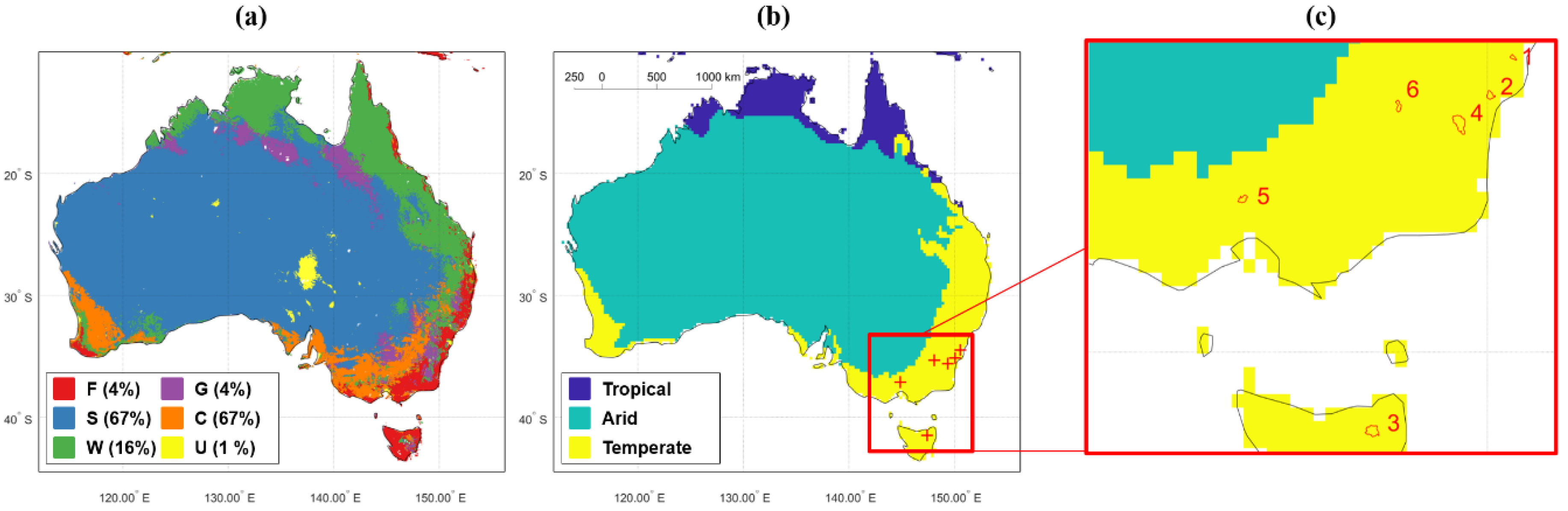
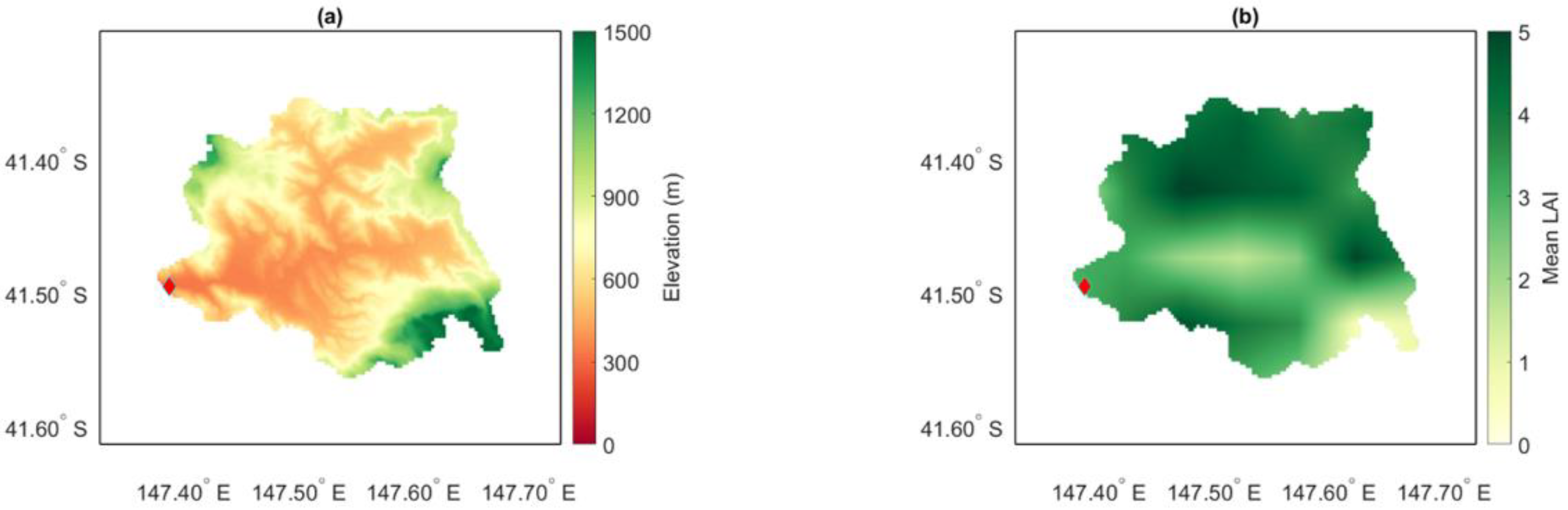
2.1. Study Area
2.2. Remote Sensing and Forcing Datasets
2.3. Description of SMART
2.4. Proposed LAI Parameterization Method
2.5. Hydrologic Modeling Scenarios and Evaluation Metrics
3. Results and Discussion
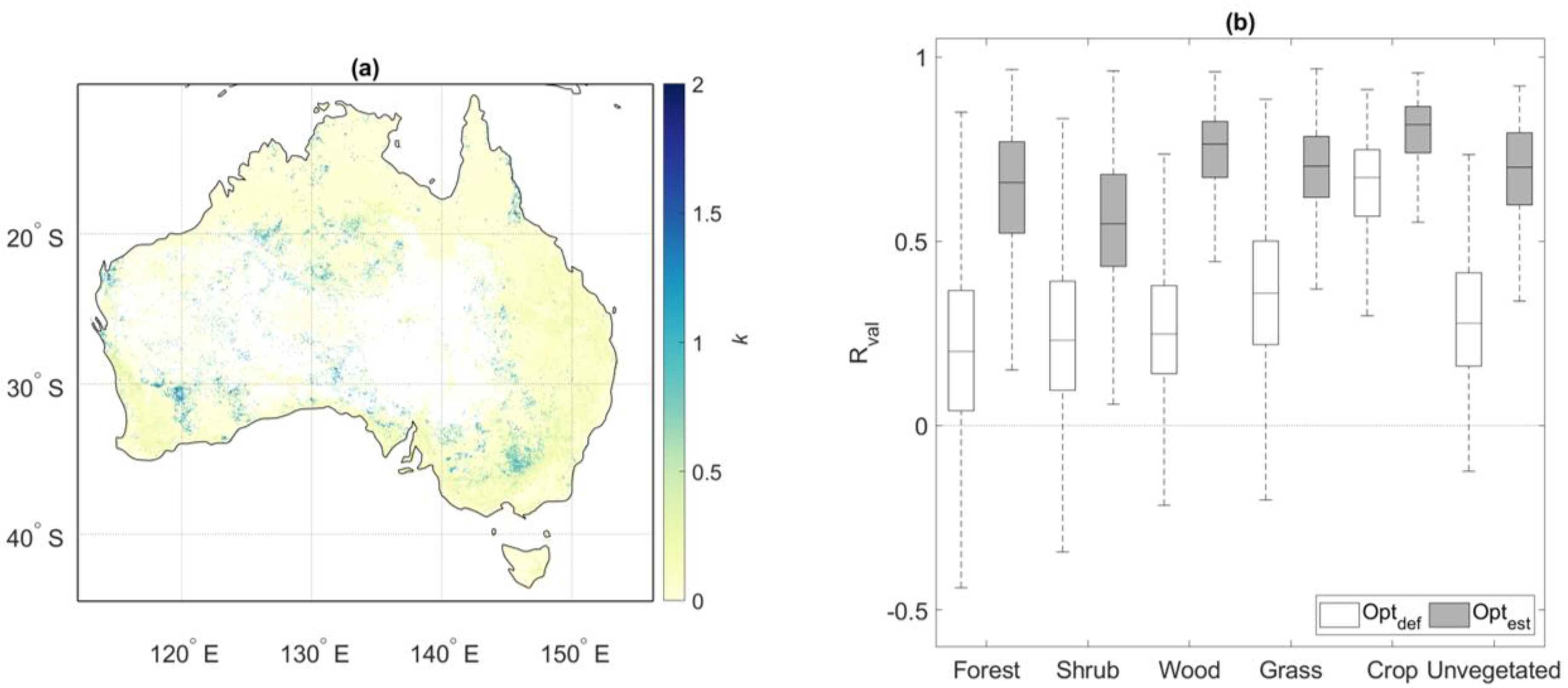
3.1. Results of LAI Modelling
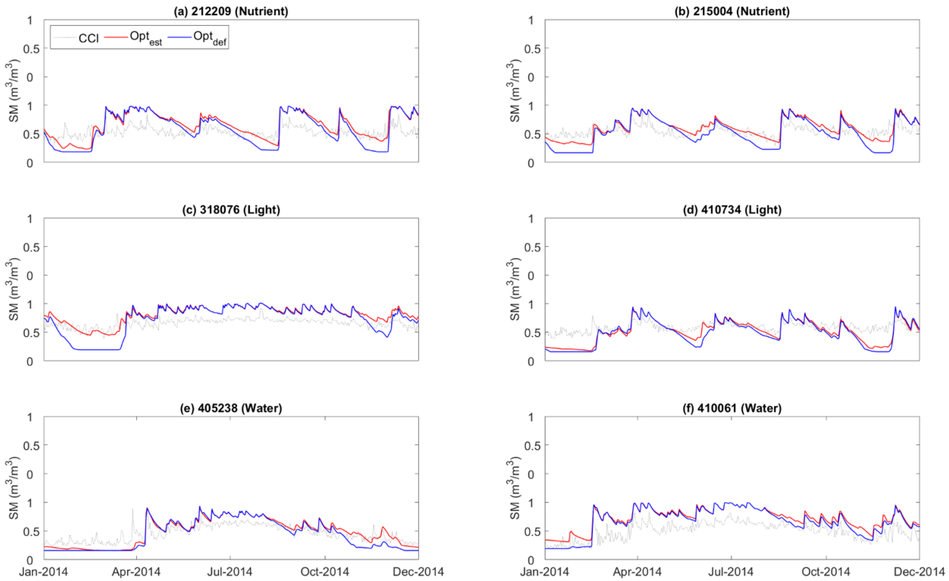
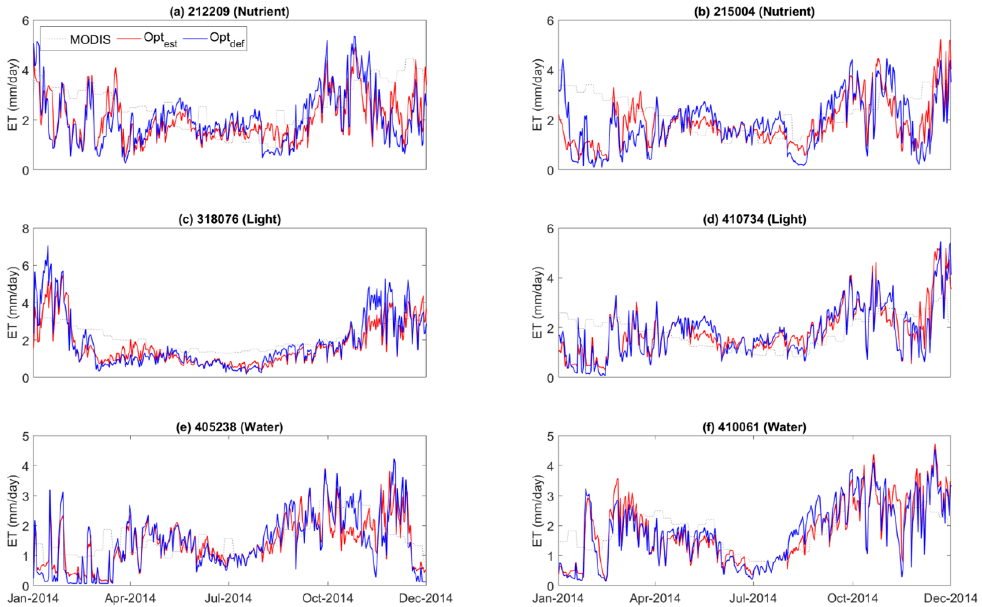
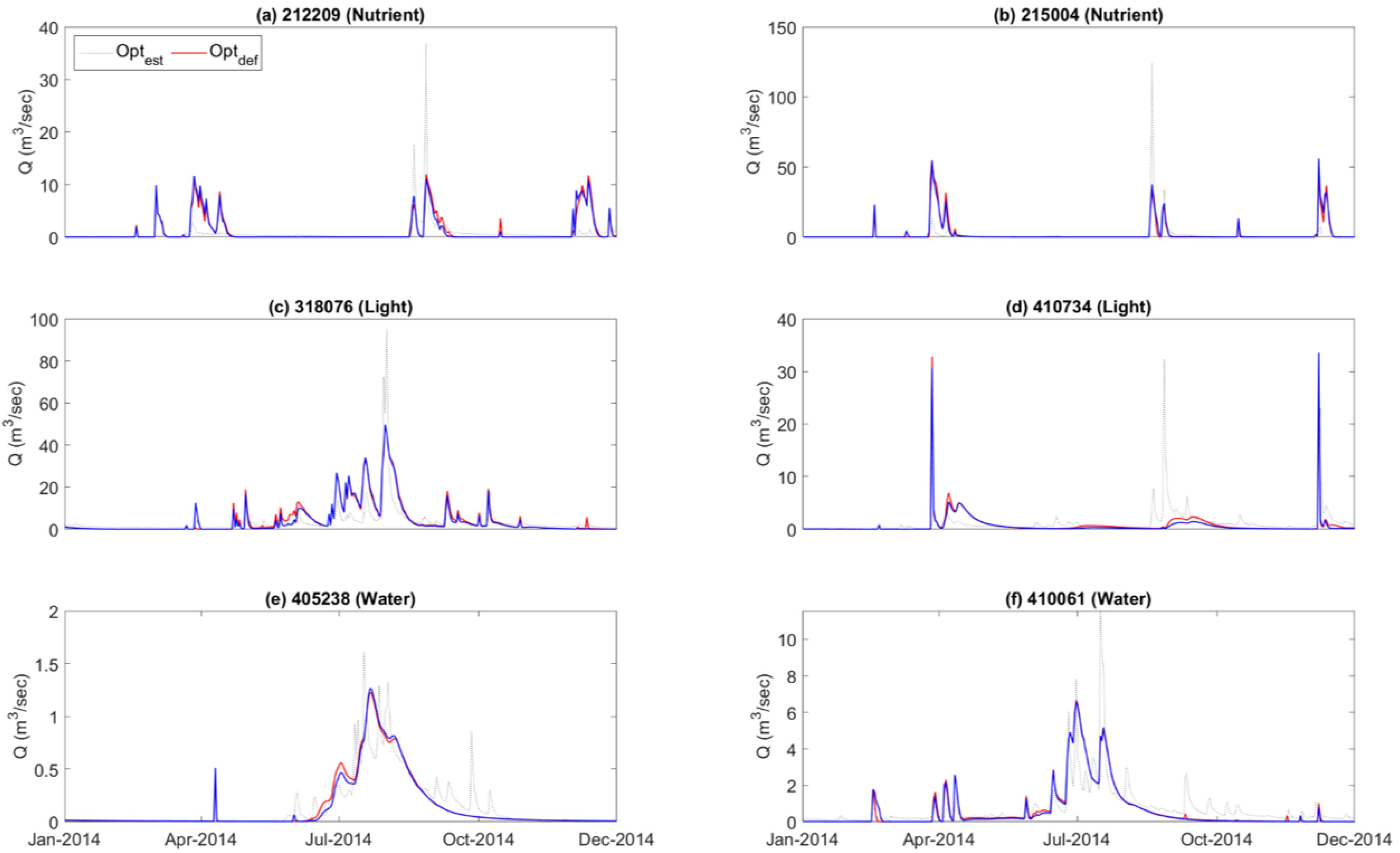
3.2. Results of Catchment-Scale Simulations of SM, ET and Q
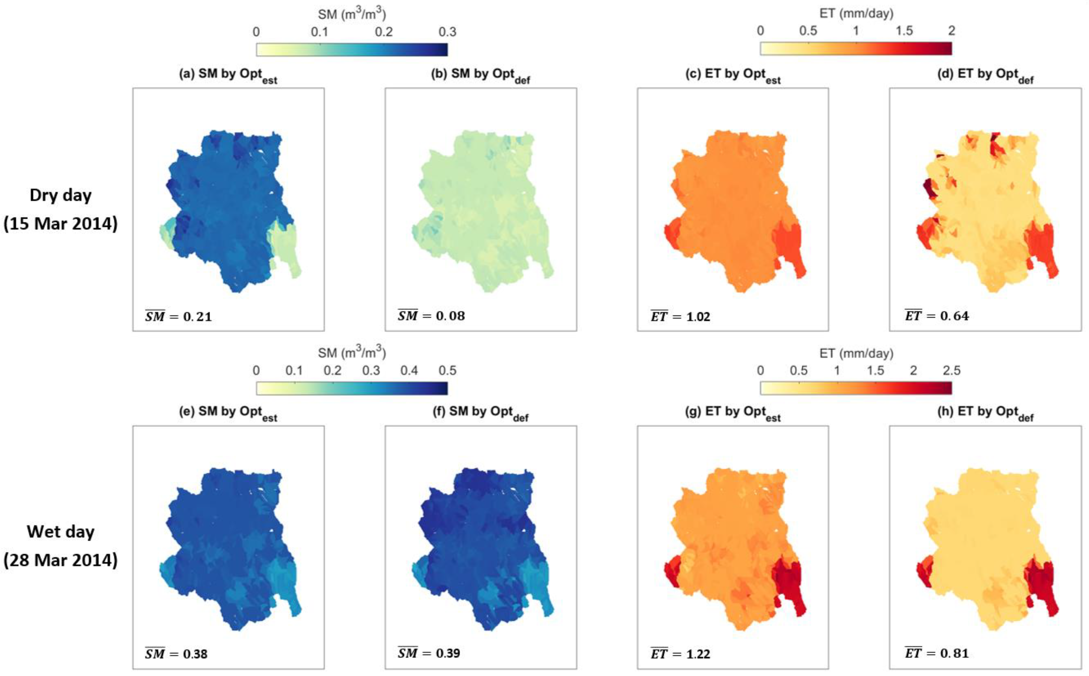
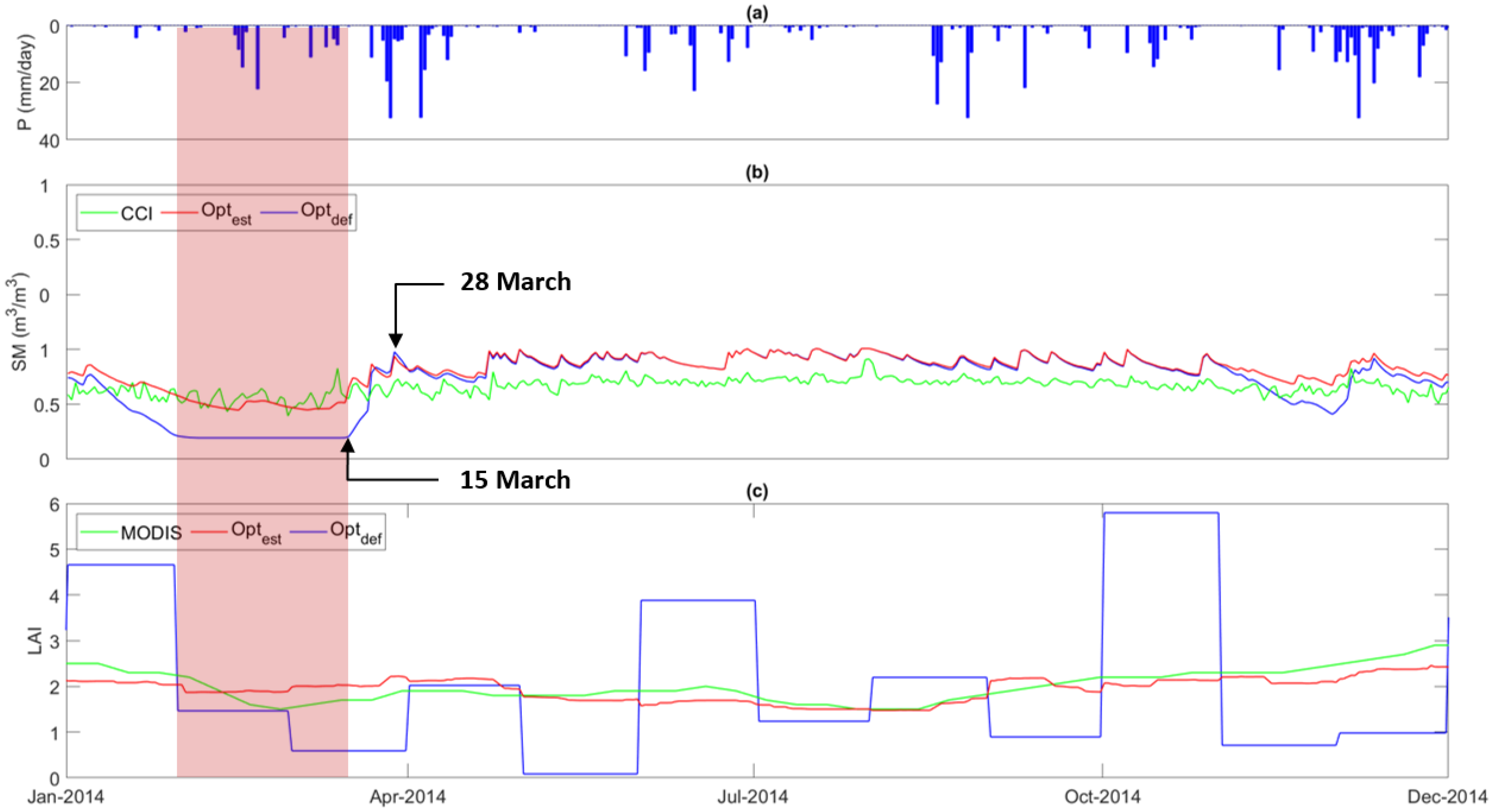
3.3. Saptial Variability of SM and ET
3.4. Caveats and Follow-Up Studies
4. Conclusions
Author Contributions
Funding
Acknowledgments
Conflicts of Interest
References
- Ukkola, A.M.; Keenan, T.F.; Kelley, D.I.; Prentice, I.C. Vegetation plays an important role in mediating future water resources. Environ. Res. Lett. 2016, 11, 094022. [Google Scholar] [CrossRef] [Green Version]
- Bonan, G.B.; Pollard, D.; Thompson, S.L. Effects of boreal forest vegetation on global climate. Nature 1992, 359, 716–718. [Google Scholar] [CrossRef]
- Yuan, X.; Wang, W.; Cui, J.; Meng, F.; Kurban, A.; De Maeyer, P. Vegetation changes and land surface feedbacks drive shifts in local temperatures over Central Asia. Sci. Rep. 2017, 7, 3287. [Google Scholar] [CrossRef] [PubMed] [Green Version]
- Tesemma, Z.K.; Wei, Y.; Peel, M.C.; Western, A.W. The effect of year-to-year variability of leaf area index on Variable Infiltration Capacity model performance and simulation of runoff. Adv. Water Resour. 2015, 83, 310–322. [Google Scholar] [CrossRef] [Green Version]
- Peel, M.C. Hydrology: Catchment vegetation and runoff. Prog. Phys. Geogr. Earth Environ. 2009, 33, 837–844. [Google Scholar] [CrossRef]
- Yang, C.; Yu, Z.; Hao, Z.; Lin, Z.; Wang, H. Effects of Vegetation Cover on Hydrological Processes in a Large Region: Huaihe River Basin, China. J. Hydrol. Eng. 2013, 18, 1477–1483. [Google Scholar] [CrossRef]
- Ajami, H.; Sharma, A.; Band, L.E.; Evans, J.P.; Tuteja, N.K.; Amirthanathan, G.E.; Bari, M.A. On the non-stationarity of hydrological response in anthropogenically unaffected catchments: An Australian perspective. Hydrol. Earth Syst. Sci. 2017, 21, 281–294. [Google Scholar] [CrossRef] [Green Version]
- Tague, C.; Band, L. RHESSys: Regional Hydro-Ecologic Simulation System—An object-oriented approach to spatially distributed modeling of carbon, water, and nutrient cycling. Earth Interact. 2004, 8, 1–42. [Google Scholar] [CrossRef]
- Fatichi, S.; Ivanov, V.; Caporali, E. A mechanistic ecohydrological model to investigate complex interactions in cold and warm water-controlled environments: 1. Theoretical framework and plot-scale analysis. J. Adv. Model. Earth Syst. 2012, 4. [Google Scholar] [CrossRef]
- Tang, Y.; Marshall, L.; Sharma, A.; Ajami, H. A Bayesian alternative for multi-objective ecohydrological model specification. J. Hydrol. 2018, 556, 25–38. [Google Scholar] [CrossRef]
- Asbjornsen, H.; Goldsmith, G.R.; Alvarado-Barrientos, M.S.; Rebel, K.; Van Osch, F.P.; Rietkerk, M.; Chen, J.; Gotsch, S.; Tobón, C.; Geissert, D.R.; et al. Ecohydrological advances and applications in plant–water relations research: A review. J. Plant Ecol. 2011, 4, 3–22. [Google Scholar] [CrossRef]
- Donohue, R.; Roderick, M.; McVicar, T.R. On the importance of including vegetation dynamics in Budyko? s hydrological model. Hydrol. Earth Syst. Sci. Discuss. 2006, 3, 1517–1551. [Google Scholar] [CrossRef] [Green Version]
- Arora, V. Modeling vegetation as a dynamic component in soil-vegetation-atmosphere transfer schemes and hydrological models. Rev. Geophys. 2002, 40. [Google Scholar] [CrossRef] [Green Version]
- Wigmosta, M.S.; Vail, L.W.; Lettenmaier, D.P. A distributed hydrology-vegetation model for complex terrain. Water Resour. Res. 1994, 30, 1665–1679. [Google Scholar] [CrossRef]
- Liang, X.; Lettenmaier, D.P.; Wood, E.F.; Burges, S.J. A simple hydrologically based model of land surface water and energy fluxes for general circulation models. J. Geophys. Res. Atmos. 1994, 99, 14415–14428. [Google Scholar] [CrossRef]
- Simunek, J.J.; Šejna, M.; Saito, H.; Sakai, M.; Van Genuchten, M. The Hydrus-1D Software Package for Simulating the Movement of Water, Heat, and Multiple Solutes in Variably Saturated Media. Version 4.17, HYDRUS Software Series 3. Department of Environmental Sciences, University of California Riverside: Riverside, CA, USA, 2013. Available online: https://www.pc-progress.com/Downloads/Pgm_Hydrus1D/HYDRUS1D-4.17.pdf(accessed on 18 September 2020).
- Ritchie, J.T. Model for predicting evaporation from a row crop with incomplete cover. Water Resour. Res. 1972, 8, 1204–1213. [Google Scholar] [CrossRef] [Green Version]
- Ford, T.W.; Quiring, S.M. Influence of MODIS-derived dynamic vegetation on VIC-simulated soil moisture in Oklahoma. J. Hydrometeorol. 2013, 14, 1910–1921. [Google Scholar] [CrossRef]
- Donohue, R.J.; Roderick, M.L.; McVicar, T.R. Roots, storms and soil pores: Incorporating key ecohydrological processes into Budyko’s hydrological model. J. Hydrol. 2012, 436, 35–50. [Google Scholar] [CrossRef]
- Li, D.; Pan, M.; Cong, Z.; Zhang, L.; Wood, E. Vegetation control on water and energy balance within the Budyko framework. Water Resour. Res. 2013, 49, 969–976. [Google Scholar] [CrossRef]
- Yang, Y.; Donohue, R.J.; McVicar, T.R. Global estimation of effective plant rooting depth: Implications for hydrological modeling. Water Resour. Res. 2016, 52, 8260–8276. [Google Scholar] [CrossRef] [Green Version]
- Zhang, S.; Yang, Y.; McVicar, T.R.; Yang, D. An analytical solution for the impact of vegetation changes on hydrological partitioning within the Budyko framework. Water Resour. Res. 2018, 54, 519–537. [Google Scholar] [CrossRef]
- Wegehenkel, M. Modeling of vegetation dynamics in hydrological models for the assessment of the effects of climate change on evapotranspiration and groundwater recharge. Adv. Geosci. 2009, 21, 109–115. [Google Scholar] [CrossRef] [Green Version]
- Tang, Q.; Vivoni, E.R.; Muñoz-Arriola, F.; Lettenmaier, D.P. Predictability of evapotranspiration patterns using remotely sensed vegetation dynamics during the North American monsoon. J. Hydrometeorol. 2012, 13, 103–121. [Google Scholar] [CrossRef]
- Tesemma, Z.K.; Wei, Y.; Western, A.W.; Peel, M.C. Leaf Area Index Variation for Crop, Pasture, and Tree in Response to Climatic Variation in the Goulburn–Broken Catchment, Australia. J. Hydrometeorol. 2014, 15, 1592–1606. [Google Scholar] [CrossRef]
- Tesemma, Z.K.; Wei, Y.; Peel, M.C.; Western, A.W. Including the dynamic relationship between climatic variables and leaf area index in a hydrological model to improve streamflow prediction under a changing climate. Hydrol. Earth Syst. Sci. 2015, 19, 2821–2836. [Google Scholar] [CrossRef] [Green Version]
- Mohaideen, M.M.D.; Varija, K. Improved vegetation parameterization for hydrological model and assessment of land cover change impacts on flow regime of the Upper Bhima basin, India. Acta Geophys. 2018, 66, 697–715. [Google Scholar] [CrossRef]
- Ajami, H.; Khan, U.; Tuteja, N.K.; Sharma, A. Development of a computationally efficient semi-distributed hydrologic modeling application for soil moisture, lateral flow and runoff simulation. Environ. Modell. Softw. 2016, 85, 319–331. [Google Scholar] [CrossRef]
- Khan, U.; Ajami, H.; Tuteja, N.K.; Sharma, A.; Kim, S. Catchment Scale Simulations of Soil Moisture Dynamics Using an Equivalent Cross-Section based Hydrological Modelling Approach. J. Hydrol. 2018, 564, 944–966. [Google Scholar] [CrossRef]
- Khan, U.; Tuteja, N.K.; Ajami, H.; Sharma, A. An equivalent cross-sectional basis for semidistributed hydrological modeling. Water Resour. Res. 2014, 50, 4395–4415. [Google Scholar] [CrossRef]
- Vaze, J.; Tuteja, N.; Teng, J. CLASS Unsaturated Moisture Movement Model U3M-1D, User’s Manual; NSW Department of Infrastructure, Planning and Natural Resources: Sydney, Australia, 2004; ISBN 0-7347-5513-9. [Google Scholar]
- Friedl, M.A.; Sulla-Menashe, D.; Tan, B.; Schneider, A.; Ramankutty, N.; Sibley, A.; Huang, X. MODIS Collection 5 global land cover: Algorithm refinements and characterization of new datasets. Remote Sens. Environ. 2010, 114, 168–182. [Google Scholar] [CrossRef]
- Peel, M.C.; Finlayson, B.L.; McMahon, T.A. Updated world map of the Köppen-Geiger climate classification. Hydrol. Earth Syst. Sci. 2007, 11, 1633–1644. [Google Scholar] [CrossRef] [Green Version]
- Turner, M.; Bari, M.; Amirthanathan, G.; Ahmad, Z. Australian network of hydrologic reference stations-advances in design, development and implementation. In Proceedings of the Hydrology and Water Resources Symposium 2012, Sydney, Australia, 19–22 November 2012; pp. 1555–1564. [Google Scholar]
- Zhang, X.S.; Amirthanathan, G.E.; Bari, M.A.; Laugesen, R.M.; Shin, D.; Kent, D.M.; MacDonald, A.M.; Turner, M.E.; Tuteja, N.K. How streamflow has changed across Australia since the 1950s: Evidence from the network of hydrologic reference stations. Hydrol. Earth Syst. Sci. 2016, 20, 3947–3965. [Google Scholar] [CrossRef] [Green Version]
- Kim, S.; Zhang, R.; Pham, H.; Sharma, A. A Review of Satellite-Derived Soil Moisture and Its Usage for Flood Estimation. Remote Sens. Earth Syst. Sci. 2019. [Google Scholar] [CrossRef]
- Baldocchi, D.; Falge, E.; Gu, L.; Olson, R.; Hollinger, D.; Running, S.; Anthoni, P.; Bernhofer, C.; Davis, K.; Evans, R. FLUXNET: A new tool to study the temporal and spatial variability of ecosystem-scale carbon dioxide, water vapor, and energy flux densities. Bull. Am. Meteorol. Soc. 2001, 82, 2415–2434. [Google Scholar] [CrossRef]
- Dorigo, W.A.; Wagner, W.; Hohensinn, R.; Hahn, S.; Paulik, C.; Xaver, A.; Gruber, A.; Drusch, M.; Mecklenburg, S.; van Oevelen, P.; et al. The International Soil Moisture Network: A data hosting facility for global in situ soil moisture measurements. Hydrol. Earth Syst. Sci. 2011, 15, 1675–1698. [Google Scholar] [CrossRef] [Green Version]
- Jung, M.; Reichstein, M.; Ciais, P.; Seneviratne, S.I.; Sheffield, J.; Goulden, M.L.; Bonan, G.; Cescatti, A.; Chen, J.; de Jeu, R.; et al. Recent decline in the global land evapotranspiration trend due to limited moisture supply. Nature 2010, 467, 951. [Google Scholar] [CrossRef]
- Walker, E.; García, G.A.; Venturini, V.; Carrasco, A. Regional evapotranspiration estimates using the relative soil moisture ratio derived from SMAP products. Agric. Water Manag. 2019, 216, 254–263. [Google Scholar] [CrossRef]
- Didan, K.; Barreto-Munoz, A.; Solano, R.; Huete, A. MODIS Vegetation Index User’s Guide (MOD13 Series); Vegetation Index and Phenology Lab, The University of Arizona: Tucson, AZ, USA, 2015; pp. 1–32. [Google Scholar]
- Raupach, M.; Briggs, P.; Haverd, V.; King, E.; Paget, M.; Trudinger, C. Australian water availability project (AWAP): CSIRO marine and atmospheric research component: Final report for phase 3. In Centre for Australian Weather and Climate Research (Bureau of Meteorology and CSIRO); CSIRO Marine and Atmospheric Research: Melbourne, Australia, 2009; Volume 67. [Google Scholar]
- Read, A.; Dowling, T.; Gallant, J.; Tickle, P.K.; Wilson, N. 1 Second SRTM Derived Hydrological Digital Elevation Model (DEM-H) Version 1.0; Commonwealth of Australia (Geoscience Australia): Canberra, Australia, 2011. [Google Scholar]
- Viscarra Rossel, R.; Chen, C.; Grundy, M.; Searle, R.; Clifford, D.; Odgers, N.; Holmes, K.; Griffin, T.; Liddicoat, C.; Kidd, D. Soil and Landscape Grid National Soil Attribute Maps—Soil Depth (3" resolution)—Release 1. v4 ed.; Commonwealth Scientific and Industrial Research Organisation (CSIRO): Canberra, Australia, 2014; Available online: https://data.csiro.au/dap/landingpage?pid=csiro%3A11413 (accessed on 31 December 2013).
- Viscarra Rossel, R.; Chen, C.; Grundy, M.; Searle, R.; Clifford, D.; Odgers, N.; Holmes, K.; Griffin, T.; Liddicoat, C.; Kidd, D. Soil and Landscape Grid National Soil Attribute Maps—Sand (3" resolution)—Release 1. v4 ed.; Commonwealth Scientific and Industrial Research Organisation (CSIRO): Canberra, Australia, 2014; Available online: https://data.csiro.au/dap/landingpage?pid=csiro%3A10149 (accessed on 31 December 2013).
- Viscarra Rossel, R.; Chen, C.; Grundy, M.; Searle, R.; Clifford, D.; Odgers, N.; Holmes, K.; Griffin, T.; Liddicoat, C.; Kidd, D. Soil and Landscape Grid National Soil Attribute Maps—Clay (3" resolution)—Release 1. v4 ed.; Commonwealth Scientific and Industrial Research Organisation (CSIRO): Canberra, Australia, 2014; Available online: https://data.csiro.au/dap/landingpage?pid=csiro:10168 (accessed on 31 December 2013).
- Viscarra Rossel, R.; Chen, C.; Grundy, M.; Searle, R.; Clifford, D.; Odgers, N.; Holmes, K.; Griffin, T.; Liddicoat, C.; Kidd, D. Soil and Landscape Grid National Soil Attribute Maps—Silt (3" Resolution)—Release 1. v4 ed.; Commonwealth Scientific and Industrial Research Organisation (CSIRO): Canberra, Australia, 2014; Available online: https://data.csiro.au/dap/landingpage?pid=csiro%3A10688 (accessed on 31 December 2013).
- Frost, A.; Ramchurn, A.; Smith, A. The Bureau’s Operational AWRA Landscape (AWRA-L) Model. Melb. Bur. Meteorol. 2016, 47. Available online: http://www.bom.gov.au/water/landscape/assets/static/publications/Frost_Model_Description_Report.pdf (accessed on 31 December 2013).
- Liu, Y.Y.; Dorigo, W.A.; Parinussa, R.M.; de Jeu, R.A.M.; Wagner, W.; McCabe, M.F.; Evans, J.P.; van Dijk, A.I.J.M. Trend-preserving blending of passive and active microwave soil moisture retrievals. Remote Sens. Environ. 2012, 123, 280–297. [Google Scholar] [CrossRef]
- Dorigo, W.; Wagner, W.; Albergel, C.; Albrecht, F.; Balsamo, G.; Brocca, L.; Chung, D.; Ertl, M.; Forkel, M.; Gruber, A.; et al. ESA CCI Soil Moisture for improved Earth system understanding: State-of-the art and future directions. Remote Sens. Environ. 2017, 203, 185–215. [Google Scholar] [CrossRef]
- Gruber, A.; Dorigo, W.A.; Crow, W.; Wagner, W. Triple Collocation-Based Merging of Satellite Soil Moisture Retrievals. IEEE Trans. Geosci. Remote Sens. 2017, 55, 6780–6792. [Google Scholar] [CrossRef]
- Mu, Q.; Zhao, M.; Running, S.W. Improvements to a MODIS global terrestrial evapotranspiration algorithm. Remote Sens. Environ. 2011, 115, 1781–1800. [Google Scholar] [CrossRef]
- Dwyer, M.J.; Schmidt, G. The MODIS reprojection tool. In Earth Science Satellite Remote Sensing Vol. 2: Data, Computational Processing, and Tools; Qu, J.J., Gao, W., Kafatos, M., Murphy, R.E., Salomonson, V.V., Eds.; Tsinghua University Press: Beijing, China; Springer: Berlin/Heidelberg, Germany, 2006; pp. 162–177. [Google Scholar]
- Savitzky, A.; Golay, M.J.E. Smoothing and Differentiation of Data by Simplified Least Squares Procedures. Anal. Chem. 1964, 36, 1627–1639. [Google Scholar] [CrossRef]
- Jönsson, P.; Eklundh, L. TIMESAT—A program for analyzing time-series of satellite sensor data. Comput. Geosci. 2004, 30, 833–845. [Google Scholar] [CrossRef] [Green Version]
- Chen, J.; Jönsson, P.; Tamura, M.; Gu, Z.; Matsushita, B.; Eklundh, L. A simple method for reconstructing a high-quality NDVI time-series data set based on the Savitzky–Golay filter. Remote Sens. Environ. 2004, 91, 332–344. [Google Scholar] [CrossRef]
- Pettorelli, N.; Vik, J.O.; Mysterud, A.; Gaillard, J.-M.; Tucker, C.J.; Stenseth, N.C. Using the satellite-derived NDVI to assess ecological responses to environmental change. Trends Ecol. Evol. 2005, 20, 503–510. [Google Scholar] [CrossRef]
- Zhu, Z.; Piao, S.; Myneni, R.B.; Huang, M.; Zeng, Z.; Canadell, J.G.; Ciais, P.; Sitch, S.; Friedlingstein, P.; Arneth, A. Greening of the Earth and its drivers. Nat. Clim. Chang. 2016, 6, 791. [Google Scholar] [CrossRef]
- Garcia, D. Robust smoothing of gridded data in one and higher dimensions with missing values. Comput. Stat. Data Anal. 2010, 54, 1167–1178. [Google Scholar] [CrossRef] [Green Version]
- Wang, G.; Garcia, D.; Liu, Y.; De Jeu, R.; Dolman, A.J. A three-dimensional gap filling method for large geophysical datasets: Application to global satellite soil moisture observations. Environ. Modell. Softw. 2012, 30, 139–142. [Google Scholar] [CrossRef]
- Pham, H.T.; Kim, S.; Marshall, L.; Johnson, F. Using 3D robust smoothing to fill land surface temperature gaps at the continental scale. Int. J. Appl. Earth Obs. Geoinf. 2019, 82, 101879. [Google Scholar] [CrossRef]
- Beesley, C.; Frost, A.; Zajaczkowski, J. A comparison of the BAWAP and SILO spatially interpolated daily rainfall datasets. In Proceedings of the 18th World IMACS/MODSIM Congress, Cairns, Australia, 13–17 July 2009; p. 17. [Google Scholar]
- Gergis, J.; Gallant, A.J.E.; Braganza, K.; Karoly, D.J.; Allen, K.; Cullen, L.; D’Arrigo, R.; Goodwin, I.; Grierson, P.; McGregor, S. On the long-term context of the 1997–2009 ‘Big Dry’ in South-Eastern Australia: Insights from a 206-year multi-proxy rainfall reconstruction. Clim Chang. 2012, 111, 923–944. [Google Scholar] [CrossRef]
- Delworth, T.L.; Zeng, F. Regional rainfall decline in Australia attributed to anthropogenic greenhouse gases and ozone levels. Nat. Geosci. 2014, 7, 583–587. [Google Scholar] [CrossRef]
- Ji, F.; Ekström, M.; Evans, J.P.; Teng, J. Evaluating rainfall patterns using physics scheme ensembles from a regional atmospheric model. Theor. Appl. Climatol. 2014, 115, 297–304. [Google Scholar] [CrossRef]
- Kim, S.; Paik, K.; Johnson, F.M.; Sharma, A. Building a Flood-Warning Framework for Ungauged Locations Using Low Resolution, Open-Access Remotely Sensed Surface Soil Moisture, Precipitation, Soil, and Topographic Information. IEEE J. Sel. Top. Appl. Earth Observ. Remote Sens. 2018, 11, 375–387. [Google Scholar] [CrossRef]
- Penman, H.L. Natural evaporation from open water, bare soil and grass. Proc. R. Soc. Lond. Ser. A Math. Phys. Sci. 1948, 193, 120–145. [Google Scholar] [CrossRef] [Green Version]
- Libertino, A.; Sharma, A.; Lakshmi, V.; Claps, P. A global assessment of the timing of extreme rainfall from TRMM and GPM for improving hydrologic design. Environ. Res. Lett. 2016, 11, 054003. [Google Scholar] [CrossRef]
- Tuteja, N.K.; Vaze, J.; Murphy, B.; Beale, G. CLASS: Catchment Scale Multiple-landuse Atmosphere Soil Water and Solute Transport Model; CRC for Catchment Hydrology: Melbourne, Australia, 2004. [Google Scholar]
- Ajami, H.; Khan, U.; Tuteja, N.K.; Sharma, A. Semi-Distributed Hydrologic Modelling with Soil Moisture and Runoff Simulation Toolkit (SMART) User’s Manual. 2016. Available online: https://github.com/hooriajami/SMART (accessed on 29 November 2018).
- Peel, M.C.; Finlayson, B.L.; McMahon, T.A. Updated world map of the Köppen-Geiger climate classification. Hydrol. Earth Syst. Sci. Discuss. 2007, 4, 439–473. [Google Scholar] [CrossRef] [Green Version]
- Nash, J.E.; Sutcliffe, J.V. River flow forecasting through conceptual models part I—A discussion of principles. J. Hydrol. 1970, 10, 282–290. [Google Scholar] [CrossRef]
- Entekhabi, D.; Reichle, R.H.; Koster, R.D.; Crow, W.T. Performance Metrics for Soil Moisture Retrievals and Application Requirements. J. Hydrometeorol. 2010, 11, 832–840. [Google Scholar] [CrossRef]
- Ahlström, A.; Raupach, M.R.; Schurgers, G.; Smith, B.; Arneth, A.; Jung, M.; Reichstein, M.; Canadell, J.G.; Friedlingstein, P.; Jain, A.K.; et al. The dominant role of semi-arid ecosystems in the trend and variability of the land CO2 sink. Science 2015, 348, 895–899. [Google Scholar] [CrossRef] [Green Version]
- Poulter, B.; Frank, D.; Ciais, P.; Myneni, R.B.; Andela, N.; Bi, J.; Broquet, G.; Canadell, J.G.; Chevallier, F.; Liu, Y.Y.; et al. Contribution of semi-arid ecosystems to interannual variability of the global carbon cycle. Nature 2014, 509, 600. [Google Scholar] [CrossRef] [PubMed] [Green Version]
- Li, L.; Wang, Y.-P.; Beringer, J.; Shi, H.; Cleverly, J.; Cheng, L.; Eamus, D.; Huete, A.; Hutley, L.; Lu, X.; et al. Responses of LAI to rainfall explain contrasting sensitivities to carbon uptake between forest and non-forest ecosystems in Australia. Sci. Rep. 2017, 7, 11720. [Google Scholar] [CrossRef]
- Bobée, C.; Ottlé, C.; Maignan, F.; de Noblet-Ducoudré, N.; Maugis, P.; Lézine, A.M.; Ndiaye, M. Analysis of vegetation seasonality in Sahelian environments using MODIS LAI, in association with land cover and rainfall. J. Arid Environ. 2012, 84, 38–50. [Google Scholar] [CrossRef]
- Zhu, Z.; Bi, J.; Pan, Y.; Ganguly, S.; Anav, A.; Xu, L.; Samanta, A.; Piao, S.; Nemani, R.R.; Myneni, R.B. Global Data Sets of Vegetation Leaf Area Index (LAI)3g and Fraction of Photosynthetically Active Radiation (FPAR)3g Derived from Global Inventory Modeling and Mapping Studies (GIMMS) Normalized Difference Vegetation Index (NDVI3g) for the Period 1981 to 2011. Remote Sens. 2013, 5, 927–948. [Google Scholar]
- Javadian, M.; Behrangi, A.; Smith, W.K.; Fisher, J.B. Global Trends in Evapotranspiration Dominated by Increases across Large Cropland Regions. Remote Sens. 2020, 12, 1221. [Google Scholar] [CrossRef] [Green Version]
- Fisher, J.B.; Melton, F.; Middleton, E.; Hain, C.; Anderson, M.; Allen, R.; McCabe, M.F.; Hook, S.; Baldocchi, D.; Townsend, P.A. The future of evapotranspiration: Global requirements for ecosystem functioning, carbon and climate feedbacks, agricultural management, and water resources. Water Resour. Res. 2017, 53, 2618–2626. [Google Scholar] [CrossRef]
- Asadi Zarch, M.A.; Sivakumar, B.; Sharma, A. Assessment of global aridity change. J. Hydrol. 2015, 520, 300–313. [Google Scholar] [CrossRef]
- Fitsum, W.; Ashish, S. Should flood regimes change in a warming climate? The role of antecedent moisture conditions. Geophys. Res. Lett. 2016, 43, 7556–7563. [Google Scholar] [CrossRef]

| No | HRS ID | Class | Limited by | Area (km2) | Max Ele. (m) | P (mm) | PET (mm) | Land Cover Proportion (%) | ||||
|---|---|---|---|---|---|---|---|---|---|---|---|---|
| F | W | G | C | Total | ||||||||
| 1 | 212209 | B1 | Nutrient | 67.4 | 823 | 1159 | 1380 | 67 | 33 | - | - | 100 |
| 2 | 215004 | B1 | Nutrient | 165.6 | 915 | 815 | 1415 | 43 | 57 | - | - | 100 |
| 3 | 318076 | B2 | Light | 379.8 | 1572 | 1279 | 1204 | 88 | - | 12 | - | 100 |
| 4 | 410734 | B2 | Light | 563.7 | 1539 | 833 | 1352 | 33 | 33 | 33 | - | 100 |
| 5 | 405238 | A1 | Water | 164.1 | 773 | 756 | 1436 | 14 | - | 71 | 14 | 100 |
| 6 | 410061 | A1 | Water | 146.1 | 1000 | 1054 | 1471 | 50 | 17 | 33 | - | 100 |
| Primary Purpose | Data (link) | Source/Product Name | References | Resolution (Temp./Spa.) | Units |
|---|---|---|---|---|---|
| LAI modelling | LAI 1 | MODIS/ MCD15A2H (V006) | [41] | 8-day/0.05° | m2/m2 |
| Rainfall 2 | Bureau of Meteorology Australia/AWAP Gridded Daily Rainfall | [42] | Daily/0.05° | mm/day | |
| SMART modelling | DEM 3 | Geoscience Australia /SRTM-derived 1” Hydrologically Enforced DEM (DEM-H) (V1.0) | [43] | -/1” | m (a.s.l) |
| Land cover 1 | MODIS /MCD12C1 (V051) | [32] | Yearly/0.05° | - | |
| Climate zone | Updated world map of the Köppen-Geiger climate classification | [33] | -/0.25° | - | |
| Soil data 4 | Commonwealth Scientific and Industrial Research Organization (CSIRO)/Soil grain size distribution and depth (Release 1) | [44,45,46,47] | -/3” | - | |
| PET 2 | Bureau of Meteorology Australia /AWRA-L PET (V5.0) | [48] | Daily/0.05° | mm/day | |
| SM, ET and Q evaluation | SM 5 | ESA CCI /Active–passive combined surface SM (V04.4) | [49,50,51] | Daily/0.25° | m3/m3 |
| ET 1 | MODIS /MYD16A2 (V006) | [52] | Daily/0.05° | mm/day | |
| Q 6 | HRS/Daily discharge (~2014) | [34,35] | Daily | m3/sec |
| IGBP Class Number | IGBP Class | Primary Class | SMART Class |
|---|---|---|---|
| 1 | Evergreen needleleaf forest | Forest | Tree |
| 2 | Deciduous needleleaf forest | ||
| 3 | Evergreen broadleaf forest | ||
| 4 | Deciduous broadleaf forest | ||
| 5 | Mixed forests | ||
| 6 | Closed shrublands | Shrublands | Pasture |
| 7 | Open shrublands | ||
| 8 | Woody savannas | Woodlands | Tree |
| 9 | Savannas | ||
| 10 | Grasslands | Grasslands | Pasture |
| 11 | Permanent wetlands | / | / |
| 12 | Croplands | Croplands | Crop |
| 14 | Cropland/natural vegetation mosaics | ||
| 13 | Urban and built-up land | Unvegetated | / |
| 16 | Barren or sparsely vegetated | ||
| 15 | Permanent snow and ice | / | / |
| 17 | Water |
| Land Cover | R | k | |
|---|---|---|---|
| Forest | 0.21 ± 0.22 | 0.63 ± 0.18 | 0.05 ± 0.16 |
| Shrublands | 0.24 ± 0.21 | 0.55 ± 0.16 | 0.12 ± 0.26 |
| Woodlands | 0.25 ± 0.18 | 0.73 ± 0.13 | 0.06 ± 0.14 |
| Grasslands | 0.34 ± 0.21 | 0.69 ± 0.12 | 0.12 ± 0.18 |
| Croplands | 0.65 ± 0.15 | 0.79 ± 0.11 | 0.18 ± 0.18 |
| Unvegetated regions | 0.28 ± 0.18 | 0.67 ± 0.17 | 0.08 ± 0.19 |
| No | HRS ID | Catchment Average R b/w MODIS and Estimated LAI | Catchment Average k | |
|---|---|---|---|---|
| 1 | 212209 | 0.39 | 0.68 | 0.05 |
| 2 | 215004 | 0.26 | 0.74 | 0.02 |
| 3 | 318076 | 0.19 | 0.67 | 0.01 |
| 4 | 410734 | 0.18 | 0.60 | 0.06 |
| 5 | 405238 | 0.56 | 0.77 | 0.13 |
| 6 | 410061 | 0.36 | 0.73 | 0.04 |
| HRS ID | Opt | SM | ET | Q | ||||||
|---|---|---|---|---|---|---|---|---|---|---|
| R | NSE | RMSE | R | NSE | RMSE | R | NSE | RMSE | ||
| 212209 | 0.513 | −0.847 | 0.093 | 0.440 | −0.108 | 1.142 | 0.538 | 0.075 | 2.612 | |
| 0.506 | −0.760 | 0.093 | 0.449 | −0.124 | 1.158 | 0.535 | 0.070 | 2.619 | ||
| 0.482 | −2.255 | 0.099 | 0.309 | −0.513 | 1.331 | 0.529 | 0.057 | 2.637 | ||
| 215004 | 0.570 | −0.550 | 0.061 | 0.310 | −0.482 | 1.028 | 0.561 | 0.117 | 8.319 | |
| 0.576 | −0.534 | 0.060 | 0.311 | −0.508 | 1.034 | 0.559 | 0.114 | 8.331 | ||
| 0.511 | −2.796 | 0.073 | 0.147 | −1.017 | 1.195 | 0.540 | 0.075 | 8.514 | ||
| 318076 | 0.714 | −0.069 | 0.077 | 0.755 | 0.175 | 0.750 | 0.794 | 0.580 | 6.533 | |
| 0.714 | −0.068 | 0.077 | 0.755 | 0.165 | 0.757 | 0.795 | 0.582 | 6.514 | ||
| 0.669 | −1.384 | 0.084 | 0.726 | −0.321 | 0.902 | 0.794 | 0.584 | 6.484 | ||
| 410734 | 0.633 | −1.206 | 0.058 | 0.521 | −0.439 | 0.855 | 0.732 | 0.455 | 3.907 | |
| 0.604 | −1.307 | 0.066 | 0.526 | −0.453 | 0.860 | 0.740 | 0.470 | 3.854 | ||
| 0.540 | −1.423 | 0.088 | 0.415 | −0.870 | 0.973 | 0.804 | 0.596 | 3.365 | ||
| 405238 | 0.839 | 0.016 | 0.052 | 0.610 | −0.396 | 0.806 | 0.210 | −0.524 | 2.199 | |
| 0.829 | 0.040 | 0.051 | 0.633 | −0.391 | 0.805 | 0.191 | −0.564 | 2.215 | ||
| 0.800 | −0.444 | 0.065 | 0.634 | −0.727 | 0.897 | 0.212 | −0.540 | 2.170 | ||
| 410061 | 0.813 | 0.098 | 0.100 | 0.680 | −0.206 | 0.787 | 0.599 | 0.198 | 2.024 | |
| 0.804 | 0.094 | 0.101 | 0.693 | −0.191 | 0.782 | 0.603 | 0.205 | 2.015 | ||
| 0.797 | −0.098 | 0.093 | 0.635 | −0.660 | 0.910 | 0.607 | 0.215 | 2.003 | ||
© 2020 by the authors. Licensee MDPI, Basel, Switzerland. This article is an open access article distributed under the terms and conditions of the Creative Commons Attribution (CC BY) license (http://creativecommons.org/licenses/by/4.0/).
Share and Cite
Kim, S.; Ajami, H.; Sharma, A. Using Remotely Sensed Information to Improve Vegetation Parameterization in a Semi-Distributed Hydrological Model (SMART) for Upland Catchments in Australia. Remote Sens. 2020, 12, 3051. https://doi.org/10.3390/rs12183051
Kim S, Ajami H, Sharma A. Using Remotely Sensed Information to Improve Vegetation Parameterization in a Semi-Distributed Hydrological Model (SMART) for Upland Catchments in Australia. Remote Sensing. 2020; 12(18):3051. https://doi.org/10.3390/rs12183051
Chicago/Turabian StyleKim, Seokhyeon, Hoori Ajami, and Ashish Sharma. 2020. "Using Remotely Sensed Information to Improve Vegetation Parameterization in a Semi-Distributed Hydrological Model (SMART) for Upland Catchments in Australia" Remote Sensing 12, no. 18: 3051. https://doi.org/10.3390/rs12183051
APA StyleKim, S., Ajami, H., & Sharma, A. (2020). Using Remotely Sensed Information to Improve Vegetation Parameterization in a Semi-Distributed Hydrological Model (SMART) for Upland Catchments in Australia. Remote Sensing, 12(18), 3051. https://doi.org/10.3390/rs12183051