Water Volume Variations Estimation and Analysis Using Multisource Satellite Data: A Case Study of Lake Victoria

Abstract

The spatiotemporal changes of lake water resources objectively reflect not only the process of the water resources balance, but also the ecological environment changes in the lake area. In recent decades, climate changes and human activities have caused great impacts on the spatial distribution of the earth’s water resources and the spatiotemporal process of the surface water cycle, which has caused a series of ecological crises and environmental problems, such as the drying-up of inland lakes, the disappearance of the oasis, water shortage or flooding and water pollution. Therefore, monitoring and fully understanding the dynamic changes of lakes is of great scientific significance for grasping regional water balance, water resources management, and sustainable development of the ecological environment. In this study, we focus on using multi-source satellite data on the estimation of water volume and multi-timescale variations analysis for large scale lakes. This study combines the problems in the practical application of “African Water Action”, taking the largest lake in Africa, Lake Victoria, as the study area, and utilizes long-term serial multi-source satellite data of the past 15 years (2003–2017), including Moderate-resolution Imaging Spectroradiometer (MODIS), Jason-1/-2/-3 and Gravity Recovery and Climate Experiment (GRACE) to perform the comprehensive analysis on the water volume change estimation. Firstly, the satellite altimetry data of Jason-1/-2/-3 and MODIS imagery was used to calculate series of water level, and to extract series of water surface area, respectively. On this basis, a more accurate regression model between the area and water level variation ($\Delta H$) was constructed. Then, the model between water volume variation ($\Delta V$) and $\Delta H$, derived from area-$\Delta H$ model, was applied to calculate the relative water volume of Lake Victoria. Meanwhile, terrestrial water storage (TWS) changes between 2003 and 2016, derived from GRACE data, were also used for a comparative verification of the $\Delta V$ results. The results show the long-term series change trends of $\Delta V$ and the TWS are the same. Finally, the multi-timescale analysis of water volume changes was carried out on different time scales, such as the inter-annual, inter-monthly, and variation period.

1. Introduction

The spatiotemporal change of lake water resources can directly record the change of the regional ecological environment and objectively reflect the process of the regional water balance. In recent decades, the spatial distribution of the earth’s water resources and the spatiotemporal process of the surface water cycle have changed greatly, and caused a series of ecological crises [1]. In particular, the ongoing climate warming and the increasing human activities have been leading to the drying up of many inland lakes, the disappearance of the oases on earth, water storage, water pollution, and other environmental problems. Therefore, lake dynamic change monitoring has become one of the most important contents of hydrology and water resources remote sensing.

Satellite earth observation technology enables humans to acquire the geometric and physical information of the earth surface changes continuously and rapidly, and to monitor the dynamic changes of the earth surface environment. Compared with the traditional methods of lake investigation, it has obvious advantages and has become a powerful technical method of lake research. The area, water level and water volume of lakes are important indexes in the study and management of hydrology and water resources. Many scholars start with the lake area, use satellite remote sensing images and lake hydrological station observation data to study the temporal and spatial characteristics and laws of lake evolution, analyzing the response of the lake to human activities and climate change, and exploring the main factors affecting lake variation [2,3,4,5,6,7,8]. The fluctuation of lake water level can affect the ecological process and pattern of the lake in many ways. Since the development of satellite altimetry technology in 1970s, with the implementation of TOPEX /Poseidon, ENVISAT, ICESat, CryoSat-2, and other satellite missions, its application scope has gradually expanded and matured. The accuracy of height measurement of a single lake will vary according to the knowledge of range, orbit, and various corrections. In practice, then, validation exercises using ground-based gauge data can measure some degree of expected accuracy for similar target type and size. Therefore, Birkett (1995) [9] and Cre’taux (2006) [1] believe that the accuracy of satellite altimetry in large lakes can reach 3–5 cm. At present, the monitoring and response analysis of water level fluctuation have been carried out in many typical lakes and watersheds [9,10,11,12,13,14].

When analyzing the change of lake water resources, it is very important to take the lake surface area or water level as the main index. However, the storage capacity of the lake is a comprehensive index reflecting the water cycle. Usually, the change of lake water volume is applied to establish the relationship of the lake water balance, and then analyze the main control factors of water balance in different climate regions. It is of great significance to study the influence of climate change and human activities on regional water volume. Monitoring lake water volume change has become one of the most important contents of hydrology and water resources remote sensing. The traditional methods of lake water volume estimation are usually combined with lake bottom topography data or area storage model data [15,16,17,18]. However, it is difficult to obtain the bottom terrain data. Especially for large lakes, this method is time-consuming, laborious, expensive, and difficult to implement. For lakes, the total absolute water volume ($V$) is generally composed of constant water volume ($V_0$) and variable water volume ($\Delta V$). Taking the lowest level in the study period as the reference surface, the water volume below the reference surface is constant water volume, and the corresponding water volume change above the surface is the relative water volume change. For the analysis of time series, it is more meaningful to study the change of the relative water volume than to calculate the absolute water volume. Thus, many scholars combined satellite remote sensing image and satellite altimetry data to estimate the change of the lake water volume [19,20,21,22,23]. The basic process is as follows: firstly, the water level or surface height data are obtained through the processing and calculation of satellite altimetry data, and the water surface area is extracted through remote sensing images. Then, the relationship between these variables and the water volume change is established by combining the water level data and lake surface area data of the lake. Finally, the variation of relative water volume is obtained through the relationship model.

Gravity recovery and climate experience (GRACE) satellite gravimetry can also be used to estimate changes in water volume [24,25,26,27,28,29,30]. However, the spatial resolution of gravity satellite data is relatively low, usually 300–400 km, and generally suitable for water bodies with an area of more than 200,000 km². This will directly affect the accuracy of water volume change estimation of small and medium-sized lakes, and limit the application scope of gravity satellite data [26]. However, the study case of Tourian et al. [31] in the Urmia basin shows that the change of total water volume of 8 km³ can be retrieved by GRACE gravimetry, which is very significant for the mutual comparison and verification in the absence of measured hydrological and topographic data.

According to the research and development status and trend analysis, the following problems exist in the study of lake water volume change by combining multi-source satellite observation data: (1) combined with the surface area extracted from remote sensing image, there are some algorithms to be used for estimating the water volume change. However, most of the studies do not consider the geographical and climate differences of lakes, and often directly use the water volume change estimation model or the simple storage capacity model researched by others. How to establish the best regression analysis model to improve the accuracy and reliability of water volume change estimation is worth further study. (2) GRACE is limited by spatial resolution, so it is difficult to obtain reliable water volume change results in a small area. It is necessary to use remote sensing methods to study how to estimate the change of water volume on a relatively small scale.

In view of the deficiencies in the existing research, we plan to study the key technologies and methods of comprehensive analysis of multi-source spatial observation data, use multi-source satellite data to carry out water volume change estimation and multi-timescale analysis of large lakes. We take Lake Victoria, the largest lake in Africa, as an example to verify, so as to achieve rapid and accurate estimation of water volume change and reconstruction of its change process.

2. Study Area

Located at 0°20′N/3°0′S–31°40′E/34°53′E, Lake Victoria (shown in Figure 1a,b) is the largest lake in Africa and the second largest freshwater lake in the world. The lake has an irregular quadrilateral shape with an area of about 68,870 km². The lakeshore is twisted, except for the west bank, and the shoreline is longer than 3500 km. The only exit of the lake is the Victoria Nile on the north bank. With the location on the East African plateau, Lake Victoria is characterized by high precipitation and high evaporation relative to river inflow and outflow. Precipitation over the lake and evaporation from the lake are the largest terms in the water balance, with 76% of the input and 77% of the output, respectively. Lake level fluctuations over Lake Victoria and its basins are caused primarily by rainfall and dam runoff [32,33]. The annual precipitation is about 1300 mm. It has a bimodal rainfall pattern; the long rains of March–May (MAM) and short rains of September–November (SON) [30,32,34].

Lake Victoria is the boundary lake between Uganda, Tanzania, and Kenya. The lake district is one of the most densely populated areas in Africa, raising nearly 30 million people around [35]. As international waters, Lake Victoria is currently being severely affected by a variety of intertwined socio-economic activities, including over-fishing, deforestation, lake siltation caused by soil erosion, invasive alien species, industrial pollution, eutrophication, and climate change [30]. To this end, using the multi-source remote sensing data to study the relative water quantity changes and influencing factors of Lake Victoria for many years is significant for the green and sustainable development of the region.

The Characteristics of Lake Victoria are obtained from the World Lakes Website [36].

3. Data

Multi-source satellite products, including multi-spectral images, multi-mission altimetry data, and satellite gravity data, are used to investigate the multi-timescale variation of Lake Victoria, which include: (i) multi-mission altimetry data from Jason-1, -2, and -3 are utilized to measure the water level during 2003 to 2017. The ENVISAT time series of water-level variations from Global Reservoirs and Lakes Monitor (GRLM) are used to access the accuracy of water level calculation. (ii) MODIS images from 2003 to 2017 are used for the extracting water body information and calculating lake surface area. (iii) GRACE are used to estimate the terrestrial water storage (TWS) changes and comparatively verify the estimation derived from water level and surface area results.

The datasets are presented in Section 3.1, Section 3.2 and Section 3.3, and summarized in

Table 1. Summary of data in the study.

Description	Source	Study Period	Data Resolution
			Spatial	Temporal
Multi-spectral imagery	MODIS (MOD09A1) [37]	2003–2017	500 m	8 days
Multi-mission altimetry data	Jason-1 [38]	2003–2012	-	10 days
	Jason-2	2012–2016	-	10 days
	Jason-3	2016–2017	-	10 days
	GRLM_ENVI [39]	2003–2010	-	35 days
Satellite gravimetry	GRACE [40]	2003–2016	0.5° × 0.5°	1 month

.

3.1. Multi-Mission Altimetry Data

• Jason-1, -2, and -3

As follow-on missions of the successful predecessor TOPEX/Poseidon (T/P), Jason-1/-2/-3 are three altimetry missions aiming to measure the sea surface level to support climate monitoring, operational oceanography, and seasonal forecasting. The orbit design is the same as that of T/P. They have the same orbit and 10-day temporal resolution, which is able to observe the same spot frequently and important for forming independent water level time series. In addition, their Geophysical Data Record (GDR) data products are of good quality and the sea surface measurement accuracy can reach 2.5–3.4 cm [41,42,43].

We utilized GDR at pass #120 provided by Archiving Validation and Interpolation of Satellite Oceanographic Data (AVISO) [38] with the time span covering cycle 001 of Jason-1 in January 2003 to cycle 069 of Jason-3 in December 2017. The details are given in Figure 2.

• GRLM_ENVI

The Global Reservoirs and Lakes Monitor (GRLM), prepared by the U.S. Department of Agriculture’s Foreign Agricultural Service (USDA-FAS) in cooperation with the National Aeronautics and Space Administration’s (NASA) Goddard Space Flight Center (GSFC) and the University of Maryland (UMD), manipulates radar altimeter data in inland water bodies and provides the time series of water level changes for the world’s largest lakes and reservoirs. As for the largest water body, the accuracy of the resulting time series of height variations is expected to be better than 10cm rms [44], such as The Great Lakes, Lakes Victoria, and Lake Tanganyika.

GRLM program provides two datasets: TPJO and ENVI time series of water-level variations. TPJO mainly uses T/P, Jason-1, -2, and -3 satellite data, while ENVI uses ENVISAT satellite data with different orbits design and temporal resolution (35d). Therefore, GRLM_ENVI is used as reference data to validate the result of the water levels obtained from the Jason-1, -2, and -3 altimetry missions in the study.

3.2. Multi-Spectral Imagery

Water body information of large lakes, such as Lake Victoria, can be extracted using MODIS images. In this study, the 7 bands’ MOD09A1 products [37] from 2003 to 2017 are used to extract the water surface areas of Lake Victoria. The reason for this is that the 8 day composite product can provide more images than other multi-spectral images, such as Landsat (16 day), to establish the water volume estimation model. According to the availability of data and the distribution of cloud cover, a total of 208 MODIS images with less cloud cover and clear lake boundaries in the lake boundary region between 2003 and 2017 are selected to extract the lake surface area, analyze area variations of Lake Victoria, and then build the area and water level relationship.

3.3. Satellite Gravimetry

The NASA/DLR Gravity Recovery and Climate Experiment (GRACE) twin satellites, launched in 2002, provide global monthly total water storage anomalies by measuring Earth’s gravity field changes. The official GRACE Science Data System continuously releases monthly GRACE solution for three different processing centers: GeoforschungsZentrum Potsdam (GFZ), Center for Space Research at the University of Texas, Austin (CSR), and Jet Propulsion Laboratory (JPL). Only 1–2 years GRACE JPL solutions data can be used to obtain reliable TWS changes in hydrologically active areas [45]. When the basin area is larger than 4.0 × 10⁵ km², the accuracy of annual change of water storage estimated by GRACE can reach 1 cm equivalent water height [46]. In this study, we use the JPL mascon (JPL-M) solutions [40] that were recorded from 2003 to 2016 to calculate Lake Victoria’s TWS changes for the comparative validation.

4. Method

Figure 3 shows the technical route as follows: (i) Jason-1, -2, and -3 satellite altimetry data are used to obtain high-precision lake water level calculation; (ii) the lake water body information is extracted from MODIS images to calculate the lake surface area; (iii) establishing an effective relationship model between water level-area-volume variations, and obtain reliable estimation results of relative water volume changes; (iv) estimating TWS changes using GRACE products and comparatively verify with estimation derived from the relationship model; (v) analyzing multi-timescale variations of the lake.

4.1. Water Surface Level

According to the basic principle of satellite altimetry [41,42,43], the formula for calculating the level of the lake surface relative to the reference ellipsoid is:

$$H=R_{alt}-R-\Delta R$$

(1)

where $H$ is the distance of the water surface above the referenced ellipsoid, $R_{alt}$ is the distance of the satellite or altimeter above the reference ellipsoid, $R$ is the distance from the satellite to the surface of the Earth, as measured by the altimeter, and $\Delta R$ are all environmental and instrumental corrections. The GDR data provides several corrections. For inland lakes with relatively small water surfaces compared to the sea surface, those optimal correction models are not so effective and applicable. In order to make use of limited data and retain the largest amount of data, we do not completely use data editing criteria on the ocean, but adopt five corrections of dry/wet tropospheric, ionosphere, solid earth tide and pole tide [47]. The calculation formula for each observation correction is:

$$\Delta R=C_{wet}+C_{dry}+C_{iono}+C_{set}+C_{pol}$$

(2)

In the Formula (2), $C_{wet}$ is the wet tropospheric correction, $C_{dry}$ indicates the dry tropospheric correction, $C_{iono}$ indicates the ionosphere correction, $C_{set}$ indicates the solid earth tide correction, and $C_{pol}$ indicates the pole tide correction. All of these corrections are provided by the GDR. For the Jason series, the data editing criteria for this study are: (i) −3 ≤ latitude ≤ 0 (i.e., within the lake); (ii) surface_type=1, which indicates inland lake or water area; (iii) the altimeter altitude is not equal to the default value for data culling, i.e., qual_alt_1hz_range_ku = 0; (iv) the values of corrections such as the troposphere are within the valid range (

Table 2. Correction threshold editing elements of the Jason series altimetry data (Unit: m).

Variables	Content	Minimum	Maximum
$C_{wet}$	wet tropospheric correction	−0.5	−0.001
$C_{dry}$	dry tropospheric correction	−25	−1.9
$C_{iono}$	ionosphere correction	−0.4	0.04
$C_{set}$	solid earth tide correction	−1	1
$C_{pol}$	pole tide correction	−0.15	0.15

); (v) the difference between the GDR data in the same cycle and the average value of the period is within three times the error range.

After range correction and data edition, we acquire the time series of the lake surface level relative to the reference TOPEX ellipsoid. All sampling lake surface level in the same cycle are averaged to obtain the lake surface level for that day.

There are two overlapping periods over the 15 years (Figure 2). In order to eliminate the biases between two different satellite altimeters, the cross analysis between Jason-1/Jason-2 and Jason-2/Jason-3 is conducted. After the bias elimination, a unique time series of lake surface level is formed.

In order to separate $V_0$ and $\Delta V$, the lowest lake surface level $H_0$ during the study period is used as the reference water level. Then, the water level variation above lowest level ($\Delta H$) can be obtained after all lake surface levels have been subtracted from the lowest level during the study period.

4.2. Water Surface Area

The MOD09A1 product is a Level-3 product with atmosphere and radiometric calibrations. In the study, two MOD09A1 images cover the entire lake. After the preprocessing of the mosaic image, re-projection from sinusoidal (SIN) to Universal Transverse Mercator (UTM, WGS-84) and resizing the study area to the 208 MODIS images, a total of 104 images covering the entire study area are obtained. The image area is 1°N/3°S–31°E/35°E, and the image acquisition time distribution is shown in Figure 4. In some months, due to the large cloud coverage, the available data is also relatively small. The months with poor multi-spectral imagery data availability coincides with the rainy seasons, especially the short rains of SON. We assume that the poor data availability is caused by the dense clouds associated with rainfall.

The feature space consists of seven bands of MOD09A1. From a large number of algorithms that have been developed to extract water body information, the support vector machine (SVM) is selected to be applied here. SVM is a supervised learning model of simple structure, strong generalization ability by the use of kernel function, and has been widely used in the field of remote sensing land cover classification. In this study, the radial basis kernel function, which is one of the commonly used kernel functions in SVM application, is used. In order to extract water body, the image is divided into water and non-water. A total of 50 water training samples and 50 non-water samples, which are separately and randomly selected in each MODIS image, are utilized to train the classifier. The classification is carried out under the condition of penalty coefficient C = 100, Gamma in kernel function $\mathsf{\gamma }$ = 0.143.

The accuracy of surface area extraction is judged in term of the errors of omission and commission at the pixel scale, using the confusion matrix to evaluate the classification results of 104 images. A total of 30 water and non-water validation samples are also separately and randomly selected. The overall accuracy of all images is above 95%, and the kappa coefficient is above 0.93, which shows that SVM can extract water information well.

The water surface area is then calculated as follows:

$$A=pixels\times 0.25 {\mathrm{km}}^2$$

(3)

In the Formula (3), $pixels$ is the sum of the pixels identified as water within the lake boundary.

4.3. Water Volume Variations Estimation

It is well known that it is difficult to determine the absolute water volume in a lake without high-precision underwater topographical measurements. In this study, relative water volume variations ($\Delta V$) over the past 15 years are estimated. The regression analysis model for establishing the water level-area-volume variations relationship is the most commonly used method for estimating the relative water volume variations using satellite remote sensing imagery and satellite altimetry data [20,21,23]. First, according to the observation date, the lake surface area and $\Delta H$ results are selected for establishing the area-$\Delta H$ relationship model as follows:

$$A=f(H)$$

(4)

The area-$\Delta H$ relationship model is developed by using the regression analysis, and then the $\Delta V\text{-}\Delta H$ relationship can be derived from the integration of the relationship between the area and $\Delta H$ as follows:

$$V={\displaystyle \int AdH={\displaystyle \int f(H)dH}}$$

(5)

Finally, the water volume variation can be estimated from the $\Delta V\text{-}\Delta H$ relationship model and $\Delta H$ results.

5. Results and Discussion

5.1. Results of Lake Surface Level and $\Delta H$

After the data processing, we obtain 250 cycle records of Jason-1, 301 cycle records of Jason-2, and 70 continuously cycle records of Jason-3 (details shown in

Table 3. Records from the Jason series.

Source	Period	Cycles
Jason-1	2003-01-19~2009-01-21	250
Jason-2	2008-07-06~2016-09-27	301
Jason-3	2016-02-12~2017-12-27	70

). Furthermore, with linear interpolation of missing or culled cycles, we acquire continuous lake surface level observation records (Figure 5).

There are two overlapping periods over the past 15 years (Figure 2, Figure 5a): 21 cycles from July 2008 to January 2009 (Figure 5b), and 24 cycles from February 2016 to September 2016 (Figure 5c). In order to eliminate the biases between two different satellite altimeters, they are set as the average bias between the overlapping datasets. The average bias between Jason-1 and -2 is added to all Jason-1 results to eliminate the bias between them. The bias between Jason-2 and -3 is calibrated in the same way, adding the average bias between Jason-2 and -3 to all Jason-3 results. The average bias between Jason-1 and -2 is 1.61 cm and the bias between Jason-2 and -3 is 6.67 cm. After the bias elimination, a unique time series of lake surface level is formed.

On the basis of eliminating the systematic bias, the maximum lake surface level observed is 1119.61 m, which appeared on 11 May 2016, and the minimum surface level was 1117.30 m, appeared on 21 October 2006. The maximum change in the lake surface level over the 15 years is 2.31 m. By subtracting the lowest water level from all the results, the $\Delta H$ is obtained (Figure 6).

The water level shows a slight increase (0.0114 m/a) of a total of 0.17 m from 2003 to 2017 (Figure 6). This trend shows a sharp decrease (−1.30 m) during 2003 to 2006, followed by a sudden increase (0.74 m) at the end of 2006. There is a stable period during 2007 to 2011 and then a significant increase of 1.26 m during 2012 to 2016. Finally, there has been a decreasing trend since June 2016.

In order to validate the results, we compare our $\Delta H$ results with the GRLM_ENVI dataset. Since the GRLM_ENVI lake height variations are respective to ENVISAT reference cycle #44 mean level, while the $\Delta H$ refers to the lowest lake surface level observation during the study period, the GRLM_ENVI dataset is also processed by subtracting the lowest level from all the variations. Figure 6 shows the results after processing, both curves exhibit the same tendency and agree well from 2003 to 2010. The average error is ~2.5 cm. This error might be caused due to differences in processing method and data version.

5.2. Results of Lake Surface Area

Since the time distribution of the acquired MODIS images is not uniform (Figure 4), the area is analyzed by comparing the maximum and minimum area of the year. Figure 7 shows the comparison of the every-year maximum and minimum areas extracted from available 104 images from 2003 to 2017. The maximum area of the lake is 66,176.25 km², which occurred on 11 July 2016, while the minimum is 65,700.25 km², which occurred on 18 June 2006. The mean surface area of Lake Victoria over the past 15 years (2003–2017) is 65,925.97 km². During this period, the maximum surface area change of the lake is more than 470 km². The largest change in a year can reach 276.5 km², which occurred in 2015.

5.3. Results of Water Volume Variations Estimation

5.3.1. $\mathrm{Area}\text{-}\Delta H$ and $\Delta V\text{-}\Delta H$ Relationship Models

A total of 55 pairs of observations with similar observation dates (before or after 2 days) are selected for fitting the relationship function. Lacking field measurement data to verify the relationship, 49 pairs are randomly selected for the establishment of relationship model, and the rest 6 pairs are used to evaluate the model accuracy.

Based on linear, polynomial, power, and exponential regression, four different $\mathrm{area}\text{-}\Delta H$ relationship models are established. Figure 8a–h shows their comparison.

The R² and root mean square error (RMSE) examine the degree of correlation between the two variables in the regression analysis. Among the above four $\mathrm{area}\text{-}\Delta H$ models, the exponential model has the highest R² and lowest RMSE (R² = 0.8810, RMSE = 38.45 km²), so the fitting effect is the best, that is, the water level and area of Lake Victoria are exponential in a certain range. The fitting function relationship of the best exponential model is:

$$A=a{e}^{bH}+c=422.6e^{0.3805H}+6.529\times {10}^{{}^4}$$

(6)

The remaining six pairs, which are not used to establish the relationship model, are now used to assess the model. The validation of exponential model is listed in

Table 4. Comparison of lake surface area derived from MODIS images and relationship model.

	Date	$\mathbf{\Delta }\mathit{H}/\mathbf{m}$	MODIS-Derived Area/km2	Relationship-Derived Area/km2	Absolute Error 1/km2	Relative Error 2/%
1	2003/1/9	1.4032	66,001.50	66,006.60	5.1036	0.0077
2	2004/11/8	0.6406	65,842.25	65,825.06	17.1926	0.0261
3	2005/4/15	0.7650	65,919.00	65,851.20	67.8006	0.1029
4	2007/12/11	0.8264	65,936.00	65,864.55	71.4497	0.1084
5	2013/1/17	1.4976	66,045.75	66,032.96	12.7886	0.0194
6	2017/6/10	1.5920	66,023.75	66,060.27	36.5155	0.0553

¹ Absolute error = MODIS-derived area − relationship-derived area. ² Relative error = (MODIS-derived area − Relationship-derived area)/MODIS-derived area.

, by comparing the area derived from MODIS images and the one derived from the exponential relationship model. The absolute error average is about 35.1418 km², the relative error average is about 0.0533%, indicating that the area calculated by the relationship is basically consistent with the areas from MODIS images. The Formula (6) can effectively describe the relationship between area and $\Delta H$.

Therefore, the $\Delta V\text{-}\Delta H$ relationship is established by integration as follows:

$$V={\displaystyle \int (a{e}^{bH}+c)dH=\frac{a}{b}{e}^{bH}+cH=1110.6439e^{0.3805H}+6.529H\times {10}^4}$$

(7)

5.3.2. Water Volume Variations over the Past 15 Years

According to the $\Delta V\text{-}\Delta H$ relationship and the $\Delta H$ time series, the water volume variations of Lake Victoria over the past 15 years are estimated (Figure 9). The estimated maximum water volume variation during the 15 years was 152.9 km³. The minimum relative water volume appears on 21 October 2006, with the maximum relative water volume appearing on 11 May 2016.

Due to the limited spatial and temporal resolution of GRACE, the area of Lake Victoria in our study is relatively low, and it is difficult to use GRACE data to estimate the water volume to achieve the required accuracy. Thus, GRACE-derived TWS changes are used to verify comparatively the estimated relative water volume variations. The validation result is presented in Figure 9. GRACE-derived TWS changes from 2003 to 2016 in Lake Victoria match well with the relationship-derived $\Delta V$. Both curves exhibit the same tendency, indicating that $\Delta V$ results effectively represent water volume variation of Lake Victoria from 2003 to 2017.

5.3.3. Multi-Timescale Analysis

• Annual period of long time series:

From the overall trend (Figure 10), the year with the minimum $\Delta V$ is in 2006, and its $\Delta V$ accounts for 24% of the multi-year average. The maximum one occurs in 2016, with a $\Delta V$ of 175% of the multi-year average. The fluctuations in lake water volume for the period 2003-2017 shown in Figure 10a,b) can be divided into four periods: (1) sharp drop from 2003 to 2006 (−22.83 km³/a); (2) relatively stable from 2007 to 2011 (1.17 km³/a); (3) the gradual increase from 2012 to 2015 (12.06 km³/a); and (4) sharp decrease from 2016 to 2017 (−29.41 km³/a).

• Monthly:

Then, the monthly time series of the relative water volume of the lake and its changes is calculated (Figure 11).

The monthly average of Lake Victoria’s water volume variations (Figure 12a,b) shows that there is a bimodal pattern in intra-annual water volume variations. As precipitation has a large seasonal variation with obvious bimodal changes, climate conditions have a great influence on water volume variations of Lake Victoria. The intra-annual analysis of $\Delta V$ is presented in Figure 12a,b), where the bimodal pattern coincides with the rainy seasons. Water volume peaks in May and December, respectively, after the long rains of MAM and the short rains of SON, while the valley is reached in October and February (Figure 12b).

After investigating the occurrence time of the maximum and minimum $\Delta V$ in the past 15 years, the distribution results (Figure 13) show that the annual maximum $\Delta V$ generally appears in April to June and December, while 8 of the 15 years appear in May. February, March, and August to December are the months with the minimum $\Delta V$. Considering the bimodal raining pattern of Lake Victoria, we found that the $\Delta V$ peaks after the rains in Figure 12b.

• Variation period (cycles):

The wavelet analysis is used to understand the time-frequency structure of the lake. As a combination of trigonometric and Gaussian functions, the Morlet wavelet is widely used in the geophysical and geodetic data analysis. The periodic variations of time series can be shown by using wavelet analysis. Based on the monthly time series, the Morlet wavelet is used to calculate the result of wavelet analysis of Lake Victoria (Figure 14).

The contour map of the wavelet coefficient real part (Figure 14a) and the curve of wavelet variance (Figure 14b) can reflect the distribution of wave energy on a period scale of water volume time series, and can be used to determine the main period existing in the process of water volume evolution. There are three peaks in the wavelet variance curve, which correspond to the period scales of 18, 9, and 6 months in turn. Among them, the maximum peak corresponds to the period scale of 18 months, indicating that the cycle oscillation of about 18 months (1.5a) is the strongest, which is the first main cycle of water volume change; the 9 month (0.75a) period scale corresponds to the second peak, which is the second main cycle of water volume change.

6. Conclusions

The lake’s water storage capacity is a comprehensive indicator of the water cycle reaction. The change of lake water volume is the main factor to establish the relationship of lake water balance, and to analyze the water balance in different climate regions. It is of great scientific significance to study the impact of climate change and human activities on the regional water cycle. In this study we have applied multi-sourced MODIS images (2003–2017), Jason-1, -2, and -3 altimetry data of the past 15 years (2003–2017) together with GRACE data (2003–2016) to analyze Lake Victoria’s water volume variations. Satellite radar altimetry has the ability of real-time, all-weather monitoring of Lake Victoria water level changes. Remote sensing imagery provides long-term time series of lake water area change information in a large range. Based on the time series of the water level and area, the relationship model of the $\mathrm{area}\text{-}\Delta H\text{-}\Delta V$ is established to estimate the variation of the relative water volume, which provides an improvement from a two-dimensional area and water level to a three-dimensional water volume. With the support of GRACE data, the variation estimates of TWS changes and relative water volume variation are compared and mutually verified. Each type of satellite observation data could provide valuable and unique information on different aspects of the hydrological situation of Lake Victoria. The analysis with the combination of these three satellite data comprehensively provides effective research of the hydrological conditions in this area.

The results of the study indicated that:

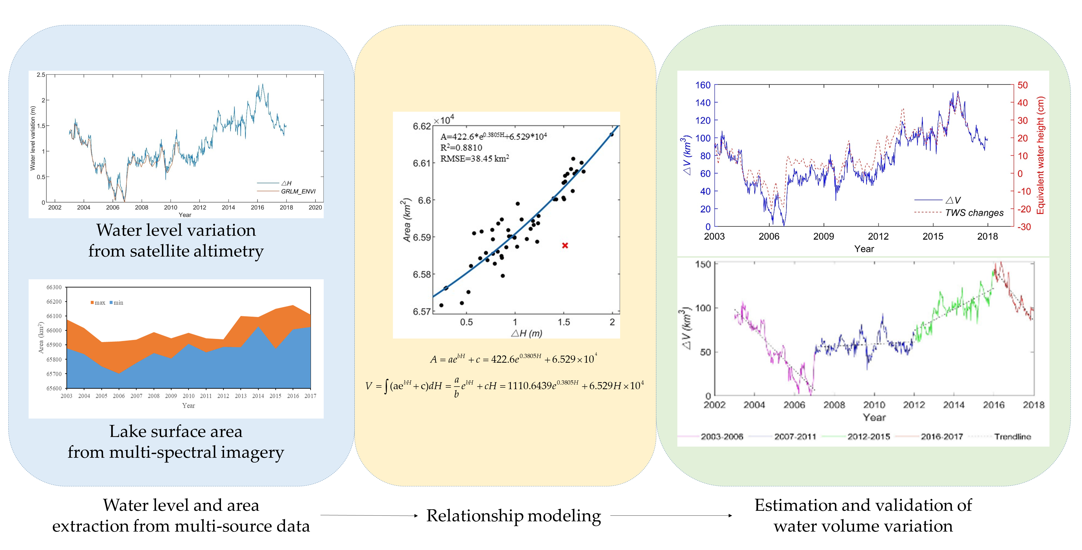
• The maximum lake surface level observed is 1119.61 m, which appears on 11 May 2016, and the minimum surface level is 1117.30 m, which appears on 21 October 2006. The maximum change in water level in the 15 years is 2.31m.
• The maximum area of the lake is 66,176.25 km², occurred on 11 July 2016, while the minimum is 65,700.25 km², occurred on 18 June 2006. The average surface area of Lake Victoria over the past 15 years (2003–2017) is 65,925.97 km². During this period, the maximum surface area of the water changes by more than 1700 km². The largest change in one year reaches 276.5 km².
• Lake water level is an important parameter for the relationship between lake area and water volume. At the same time, there are significant correlations between $\mathrm{area}\text{-}\Delta H$ and $\Delta V\text{-}\Delta H$. The simulation analysis of four models, linear, polynomial, power, and exponential, determine that the relationship between the area of Lake Victoria and the water level are exponential in a certain range. The exponential model has the highest correlation coefficient (R² = 0.8810, RMSE = 38.45).

After completing the estimation of water level, area, and water volume variation, a multi-timescale analysis of water volume changes has been estimated and the following points can also be summarized:

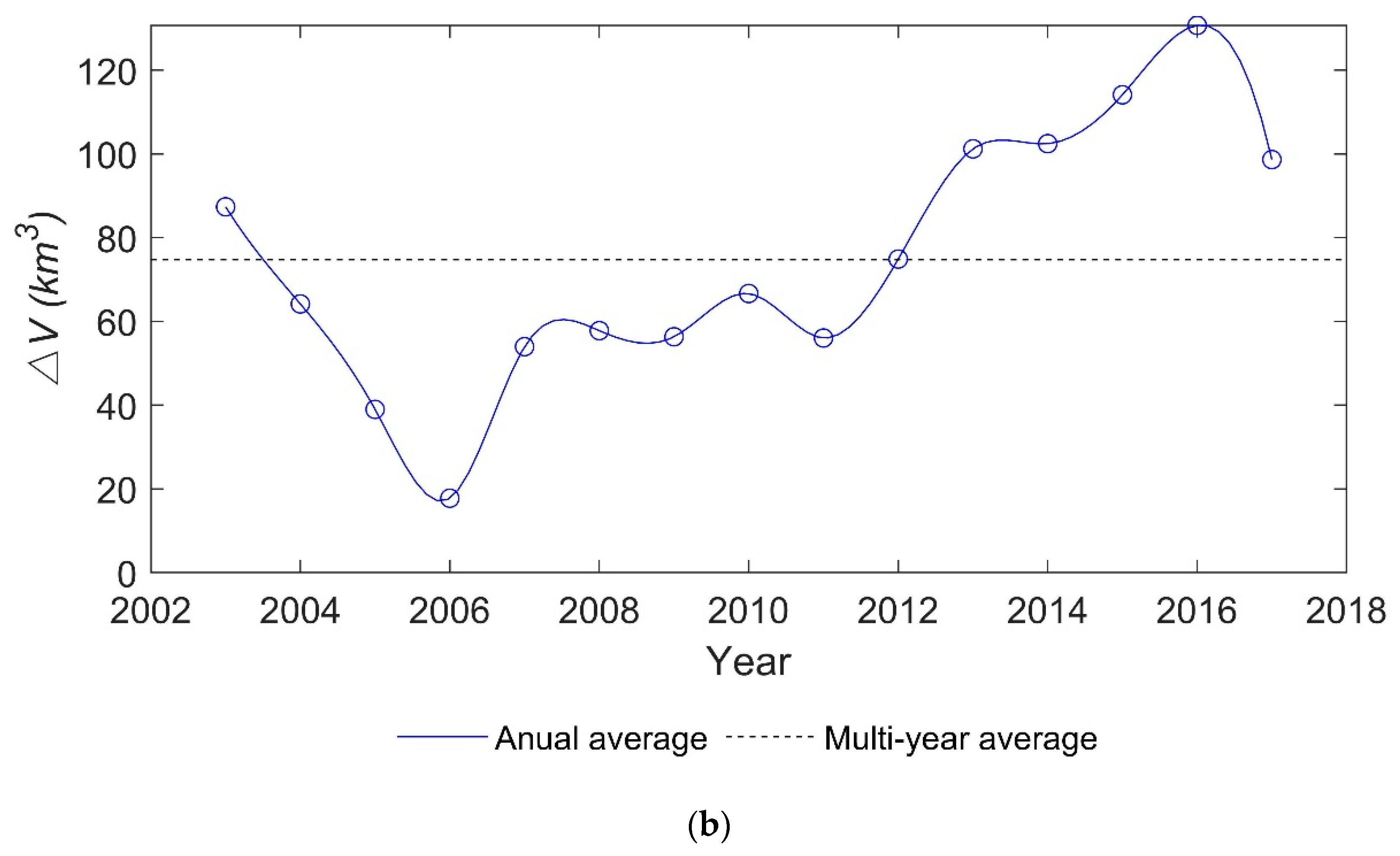
• The estimated maximum water volume variation during the 15 years is 152.9 km³. The relationship-derived water volume variations match well with the GRACE-derived TWS changes. The $\Delta V$ shows an increase trend over the past 15 years and its fluctuations can be divided into four periods: (1) sharp drop from 2003 to 2006; (2) relatively stable from 2007 to 2011; (3) gradual increase from 2012 to 2016; and (4) sharp drop from 2016 to 2017.
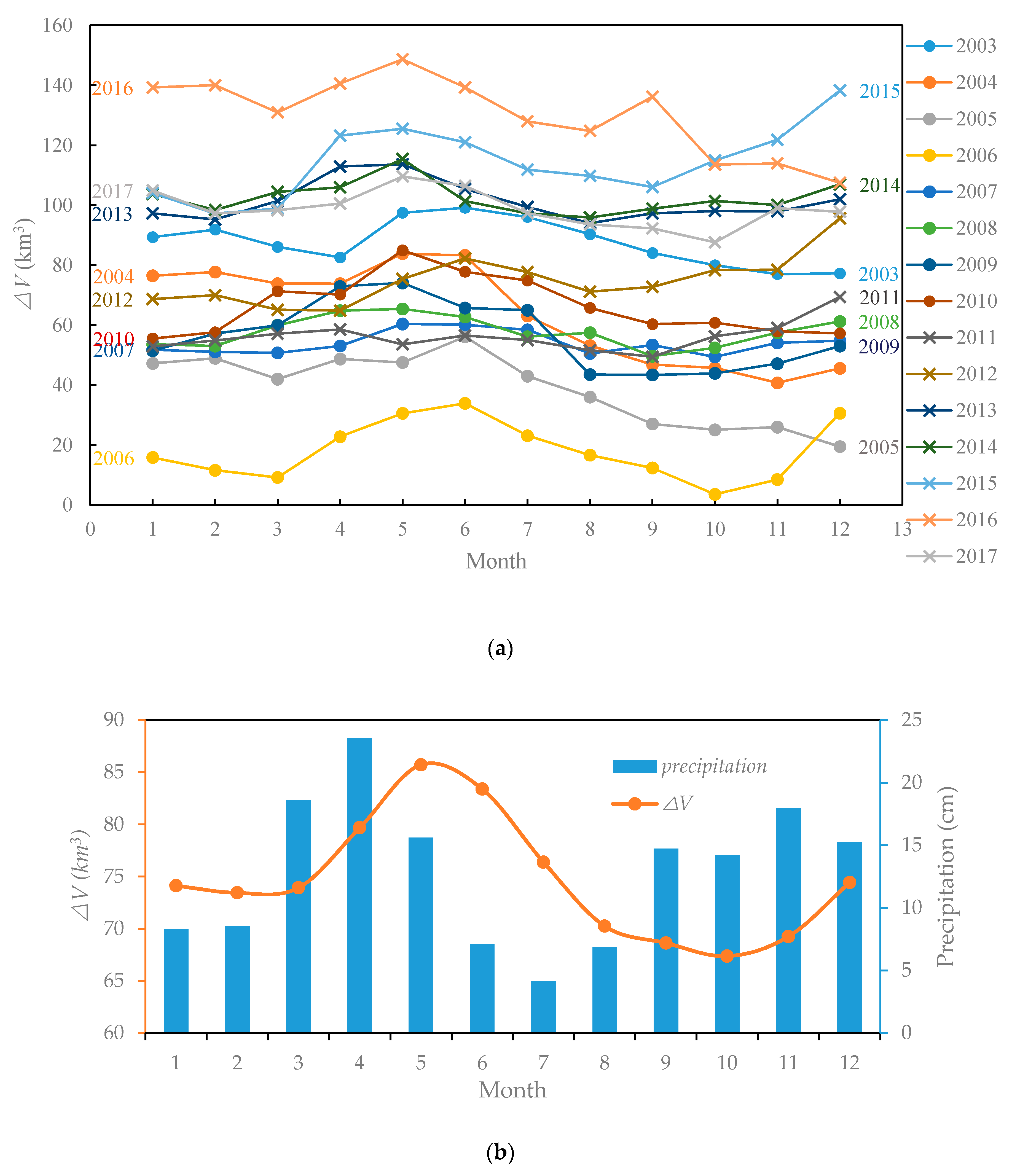
• There is a bimodal pattern in the intra-annual water volume variations, which is consistent with the changes in precipitation. As precipitation has a large seasonal variation with obvious bimodal changes, climate conditions have a great influence on water volume of Lake Victoria.
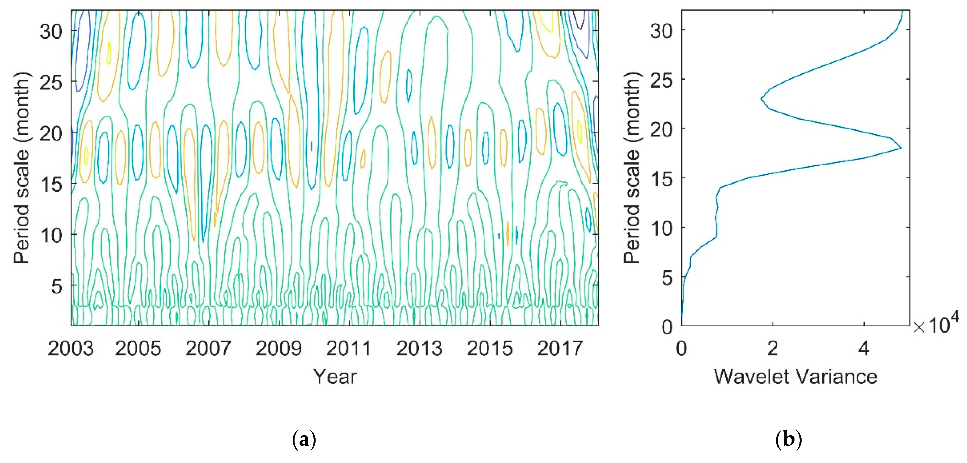
• After using Morlet wavelet to study the lake variation period, we found that the first main cycle of water volume change is 18 months (1.5 a) over the past 15 years, while the second main cycle is 9 months (0.75 a).

In this study, the time series water levels, surface area and water volume have been monitored with Jason-1/-2/-3 satellite altimetry data, MODIS images and GRACE data from 2003 to 2017. Under the influence of global climate change and human activities, our study results are of great scientific significance to timely grasp the regional water balance, sustainable use of water resources, disaster warning, and environmental protection.

Based on the above research, it is also necessary to study the large lake’s physical dynamic change associated with climate change and human activities by utilizing higher resolution remote sensing data and hydrological data. Therefore, in further study, we will concentrate on quantitative analysis of driving factors using more multiple data sources, such as meteorological data, population data, land use data, and socio-economic data.

References

1. Crétaux, J.F.; Birkett, C. Lake Studies from Satellite Radar Altimetry. Comptes Rendus Geosci. 2006, 338, 1098–1112. [Google Scholar] [CrossRef]
2. Forsythe, K.W.; Schatz, B.; Swales, S.J.; Ferrato, L.J.; Atkinson, D.M. Visualization of lake mead surface area changes from 1972 to 2009. ISPRS Int. J. Geo Inf. 2012, 1, 108–119. [Google Scholar] [CrossRef]
3. Zhang, G.Q.; Yao, T.D.; Chen, W.F.; Zheng, G.X.; Shum, C.K.; Yang, K.; Piao, S.L.; Sheng, Y.W.; Yi, S.; Li, J.L.; et al. Regional differences of lake evolution across China during 1960s–2015 and its natural and anthropogenic causes. Remote Sens. Environ. 2019, 221, 386–404. [Google Scholar] [CrossRef]
4. Feng, L.; Hu, C.; Chen, X.; Cai, X.; Tian, L.; Gan, W. Assessment of inundation changes of Poyang Lake using MODIS observations between 2000 and 2010. Remote Sens. Environ. 2012, 121, 80–92. [Google Scholar] [CrossRef]
5. Cre’taux, J.-F.; Letolle, R.; Calmant, S. Investigations on Aral Sea regressions from mirabilite deposits and remote sensing. Aquat. Geochem. 2009, 15, 277–291. [Google Scholar] [CrossRef]
6. De Wit, M.; Stankiewicz, J. Changes in surface water supply across Africa with predicted climate change. Science 2006, 311, 1917–1921. [Google Scholar] [CrossRef] [Green Version]
7. Adrian, R.; O’Reilly, C.M.; Zagarese, H.; Baines, S.B.; Hessen, D.O.; Keller, W.; Livingstone, D.M.; Sommaruga, R.; Straile, D.; Van Donk, E.; et al. Lakes as sentinels of climate change. Limnol. Oceanogr. 2009, 54, 2283–2297. [Google Scholar] [CrossRef]
8. Abileah, R.; Vignudelli, S.; Scozzari, A. A completely remote sensing approach to monitoring reservoirs water volume. Int. Water Technol. J. 2011, 1, 63–77. [Google Scholar]
9. Birkett, C.M. The global remote sensing of lakes, wetlands and rivers for hydrological and climate research. Quant. Remote Sens. Sci. Appl. 1995, 3, 1979–1981. [Google Scholar] [CrossRef]
10. Birkett, C.M.; Beckley, B. Investigating the Performance of the JASON-2/OSTM Radar Altimeter over Lakes and Reservoirs. Mar. Geod. 2010, 33, 204–238. [Google Scholar] [CrossRef]
11. Frappart, F.; Minh, K.D.; L’Hermitte, J.; Cazenave, A.; Ramillien, G.; Le Toan, T.; Mognard-Campbell, N. Water volume change in the lower Mekong from satellite altimetry and imagery data. Geophys. J. Int. 2006, 167, 570–584. [Google Scholar] [CrossRef] [Green Version]
12. Baghdadi, N.; Lemarquand, N.; Abdallah, H.; Bailly, J.S. The relevance of GLAS/ICESat elevation data for the monitoring of river networks. Remote Sens. 2011, 3, 708–720. [Google Scholar] [CrossRef] [Green Version]
13. Silva, J.S.; Calmant, S.; Seyler, F.; Moreira, D.M.; Oliveira, D.; Monteiro, A. Radar altimetry aids managing gauge networks. Water Resour. Manag. 2014, 28, 587–603. [Google Scholar] [CrossRef]
14. Kleinherenbrink, M.; Lindenbergh, R.C.; Ditmar, P.G. Monitoring of lake level changes on the Tibetan Plateau and Tian Shan by retracking Cryosat SARIn waveforms. J. Hydrol. 2015, 521, 119–131. [Google Scholar] [CrossRef]
15. Furnans, J.; Austin, B. Hydrographic survey methods for determining reservoir volume. Environ. Modeling Softw. 2008, 23, 139–146. [Google Scholar] [CrossRef]
16. Wilcox, C.; Huertos, M.L. A simple, rapid method for mapping bathymetry of small wetland basins. J. Hydrol. 2005, 301, 29–36. [Google Scholar] [CrossRef]
17. Foteinopoulos, P. Cubic spline interpolation to develop contours of large reservoirs and evaluate area and volume. Adv. Eng. Softw. 2009, 40, 23–29. [Google Scholar] [CrossRef]
18. Smith, L.C.; Pavelsky, T.M. Remote sensing of volumetric storage changes in lakes. Earth Surf. Process. Landf. 2009, 34, 1353–1358. [Google Scholar] [CrossRef]
19. Frappart, F.; Seyler, F.; Martinez, J.M.; León, J.G.; Cazenave, A. Floodplain water storage in the Negro River basin estimated from microwave remote sensing of inundation area and water levels. Remote Sens. Environ. 2005, 99, 387–399. [Google Scholar] [CrossRef] [Green Version]
20. Gao, H.; Birkett, C.M.; Lettenmeir, D.P. Global monitoring of large reservoir storage from satellite remote sensing. Water Resour. Res. 2012, 48, W09504. [Google Scholar] [CrossRef] [Green Version]
21. Duan, Z.; Bastiaanssen, W.G.M. Estimating water volume variations in lakes and reservoirs from four operational satellite altimetry databases and satellite imagery data. Remote Sens. Environ. 2013, 134, 403–416. [Google Scholar] [CrossRef]
22. Arsen, A.; Cre’taux, J.F.; Berge-Nguyen, M.; del Rio, R.A. Remote sensing derived bathymetry of Lake Poopo. Remote Sens. 2014, 6, 407–420. [Google Scholar] [CrossRef] [Green Version]
23. Tong, X.Z.; Pan, H.Y.; Xie, H.; Xu, X.; Li, F.T.; Chen, L.; Luo, X.; Liu, S.J.; Chen, P.; Jin, Y.M. Estimating water volume variations in Lake Victoria over the past 22 years using multi-mission altimetry and remotely sensed images. Remote Sens. Environ. 2016, 187, 400–413. [Google Scholar] [CrossRef]
24. Tseng, K.H.; Chang, C.P.; Shum, C.K.; Kuo, C.Y.; Liu, K.T.; Shang, K.; Jia, Y.Y.; Sun, J. Quantifying Freshwater Mass Balance in the Central Tibetan Plateau by Integrating Satellite Remote Sensing, Altimetry, and Gravimetry. Remote Sens. 2016, 8, 441. [Google Scholar] [CrossRef] [Green Version]
25. Forootan, E.; Rietbroek, R.; Kusche, J.; Sharifi, M.A.; Awange, J.L.; Schmidt, M.; Omondi, P.; Famiglietti, J. Separation of large scale water storage patterns over Iran using GRACE, altimetry and hydrological data. Remote Sens. Environ. 2014, 140, 580–595. [Google Scholar] [CrossRef] [Green Version]
26. Singh, A.; Seitz, F.; Schwatke, C. Inter-annual water storage changes in the Aral Sea from multi-mission satellite altimetry, optical remote sensing, and GRACE satellite gravimetry. Remote Sens. Environ. 2012, 123, 187–195. [Google Scholar] [CrossRef]
27. Singh, A.; Seitz, F.; Schwatke, C. Application of multi-sensor satellite data to observe water storage variations. IEEE J. Sel. Top. Appl. Earth Obs. Remote Sens. 2013, 6, 1502–1508. [Google Scholar] [CrossRef]
28. Ramillien, G.; Frappart, F.; Seoane, L. Application of the regional water mass variations from GRACE satellite gravimetry to large-scale water management in Africa. Remote Sens. 2014, 6, 7379–7405. [Google Scholar] [CrossRef] [Green Version]
29. Llovel, W.; Becker, M.; Cazenave, A. Global land water storage change from GRACE over 2002–2009, inference on sea level. Comptes Rendus Geosci. 2010, 342, 179–188. [Google Scholar] [CrossRef]
30. Awange, J.L.; Anyah, R.; Agola, N.; Forootan, E.; Omondi, P. Potential impacts of climate and environmental change on the stored water of Lake Victoria Basin and economic implications. Water Resour. Res. 2013, 49, 8160–8173. [Google Scholar] [CrossRef] [Green Version]
31. Tourian, M.J.; Elmi, O.; Chen, Q.; Devaraju, B.; Roohi, S.; Sneeuw, N. A spaceborne multisensor approach to monitor the desiccation of Lake Urmia in Iran. Remote Sens. Environ. 2015, 156, 349–360. [Google Scholar] [CrossRef]
32. Vanderkelen, I.; van Lipzig, N.P.M.; Thiery, W. Modelling the water balance of Lake Victoria (East Africa) —Part 1: Observational analysis. Hydrol. Earth Syst. Sci. Discuss. 2018, 1–28. [Google Scholar] [CrossRef] [Green Version]
33. Kizza, M.; Rodhe, A.; Xu, C.Y.; Ntale, H.K.; Halldin, S. Temporal rainfall variability in the Lake Victoria Basin in East Africa during the twentieth century. Theor. Appl. Climatol. 2009, 98, 119–135. [Google Scholar] [CrossRef]
34. Nicholson, S.E. Climate and climatic variability of rainfall over eastern Africa. Rev. Geophys. 2017, 55, 590–635. [Google Scholar] [CrossRef] [Green Version]
35. Bremner, J.; Lopez-Carr, D.; Zvoleff, A.; Pricope, N. Using new methods and data to assess and address population, fertility, and environment links in the Lake Victoria Basin, Population and the environment. In Proceedings of the 2013 International Union for the Scientific Study of Population (IUSSP), Busan, Korea, 26–31 August 2013. [Google Scholar]
36. World Lakes Website. Available online: http://www.worldlakes.org/lakedetails.asp?lakeid=8361 (accessed on 1 January 2020).
37. MODIS Imagery. Available online: http://ladsweb.nascom.nasa.gov/data/search (accessed on 1 April 2018).
38. Jason-1, -2, -3 Altimetry Data. Available online: Ftp://avisoftp.cnes.fr/AVISO/pub/ (accessed on 1 March 2018).
39. GRLM Datasets. Available online: https://ipad.fas.usda.gov/cropexplorer/global_reservoir/ (accessed on 1 May 2018).
40. GRACE JPL-M Solutions. Available online: https://grace.jpl.nasa.gov/data/get-data/jpl_global_mascons/ (accessed on 12 December 2018).
41. Jason-1 Products Handbook. Available online: https://www.aviso.altimetry.fr/fileadmin/documents/data/tools/hdbk_j1_gdr.pdf (accessed on 4 December 2019).
42. OSTM/Jason-2 Products Handbook. Available online: https://www.aviso.altimetry.fr/fileadmin/documents/data/tools/hdbk_j2.pdf (accessed on 4 December 2019).
43. Jason-3 Products Handbook. Available online: https://www.aviso.altimetry.fr/fileadmin/documents/data/tools/hdbk_j3.pdf (accessed on 4 December 2019).
44. Birkett, C.; Reynolds, C.; Beckley, B.; Doorn, B. From Research to Operations: The USDA Global Reservoir and Lake Monitor. In Coastal Altimetry; Vignudelli, S., Kostianoy, A., Cipollini, P., Benveniste, J., Eds.; Springer: Berlin, Germany, 2011; pp. 19–50. [Google Scholar]
45. Wouters, B.; Bonin, J.A.; Chambers, D.P.; Riva, R.E.M.; Sasgen, I.; Wahr, J. Grace, time-varying gravity, earth system dynamics and climate change. Rep. Prog. Phys. Phys. Soc. 2014, 77, 116801. [Google Scholar] [CrossRef] [PubMed] [Green Version]
46. Swenson, S.; Famiglietti, J.; Basara, J.; Wahr, J. Estimating profile soil moisture and groundwater variations using GRACE and Oklahoma Mesonet soil moisture data. Water Resour. Res. 2008, 44, 568–569. [Google Scholar] [CrossRef] [Green Version]
47. Medina, C.E.; Gomez-Enri, J.; Alonso, J.J.; Villares, P. Water level fluctuations derived from ENVISAT Radar Altimeter (RA-2) and in-situ measurements in a subtropical waterbody: Lake Izabal (Guatemala). Remote Sens. Environ. 2008, 112, 3604–3617. [Google Scholar] [CrossRef]
Figure 1. (a) The location of Lake Victoria. (b) Lake Victoria from Google Earth.
Remotesensing 12 03052 g001
Figure 2. Jason-1, -2, and -3 altimetry data used.
Remotesensing 12 03052 g002
Figure 3. Technical route.
Remotesensing 12 03052 g003
Figure 4. Time distribution of the MODIS images used.
Remotesensing 12 03052 g004
Figure 5. (a) Lake surface level results derived from Jason-1, -2, and -3 before eliminating the systematic bias; (b) Overlapping period between Jason-1 and -2; (c) Overlapping period between Jason-2 and -3.
Remotesensing 12 03052 g005
Figure 6. Validation of the Δ H results by use of GRLM_ENVI.
Remotesensing 12 03052 g006
Figure 7. Comparison of the maximum and minimum areas of every year from 2003 to 2017 extracted from available data.
Remotesensing 12 03052 g007
Figure 8. A r e a - Δ H relationship models: (a) linear regression before excluding outliers; (b) linear regression after excluding outliers; (c) polynomial regression before excluding outliers; (d) polynomial regression after excluding outliers; (e) power regression before excluding outliers; (f) power regression after excluding outliers; (g) exponential regression before excluding outliers; (h) exponential regression after excluding outliers.
Remotesensing 12 03052 g008aRemotesensing 12 03052 g008b
Figure 9. Time series of the Δ V (2003–2017) from the Δ V - Δ H relationship and the TWS changes (2003 and 2016) from GRACE data.
Remotesensing 12 03052 g009
Figure 10. Annual period of long time series of Lake Victoria over the past 15 years: (a) water volume variations time series and (b) annual average.
Remotesensing 12 03052 g010aRemotesensing 12 03052 g010b
Figure 11. Monthly water volume variations time series of Lake Victoria (2003–2017).
Remotesensing 12 03052 g011
Figure 12. (a) Intra-annual analysis of Δ V (2003–2017); (b) monthly average of Lake Victoria’s Δ V and precipitation (2003–2017).
Remotesensing 12 03052 g012
Figure 13. Distribution of the maximum and minimum Δ V s of the lake from 2003 to 2017.
Remotesensing 12 03052 g013
Figure 14. Wavelet analysis of water volume change in Lake Victoria: (a) contour map of the wavelet coefficient real part; (b) the curve of wavelet variance.
Remotesensing 12 03052 g014