Mapping Paddy Rice Fields by Combining Multi-Temporal Vegetation Index and Synthetic Aperture Radar Remote Sensing Data Using Google Earth Engine Machine Learning Platform

Abstract

The knowledge of the area and spatial distribution of paddy rice fields is important for water resource management. However, accurate map of paddy rice is a long-term challenge because of its spatiotemporal discontinuity and short duration. To solve this problem, this study proposed a paddy rice area extraction approach by using the combination of optical vegetation indices and synthetic aperture radar (SAR) data. This method is designed to overcome the data-missing problem due to cloud contamination and spatiotemporal discontinuities of the traditional optical remote sensing method. More specifically, the Sentinel-1A SAR and the Sentinel-2 multispectral imager (MSI) Level-2A imagery are used to identify paddy rice with a high temporal and spatial resolution. Three vegetation indices, namely normalized difference vegetation index (NDVI), enhanced vegetation index (EVI), and land surface water index (LSWI), are estimated from optical bands. Two polarization bands (VH (vertical-horizontal) and VV (vertical-vertical)) are used to overcome the cloud contamination problem. This approach was applied with the random forest machine learning algorithm on the Google Earth Engine platform for the Jianghan Plain in China as an experimental area. The results of 39 experiments uncovered the effect of different factors. The results indicated that the combination of VV and VH band showed a better performance compared with other polarization bands; the average producer’s accuracy of paddy rice (PA) is 72.79%, 1.58% higher than the second one VH. Secondly, the combination of three indices also showed a better result than others, with average PA 73.82%, 1.42% higher than using NDVI alone. The classification result presented the best combination is EVI, VV, and VH polarization band. The producer’s accuracy of paddy rice was 76.67%, with the overall accuracy (OA) of 66.07%, and Kappa statistics of 0.45. However, NDVI, EVI, and VH showed better performance in mapping the morphology. The results demonstrated the method developed in this study can be successfully applied to the cloud-prone area for mapping paddy rice to overcome the data missing caused by cloud and rain during the paddy growing season.

1. Introduction

Paddy rice is one of the important grain crops in the world and plays a critical role in food security and water use assessments. This is because paddy rice fields account for about 11% of the cropland area in the world and feed over a billion people [1]. Further, nearly 30% of the world’s developed freshwater resources are used for paddy rice planting [2]. Paddy rice fields, as a critical form of artificial water body, plays a key role in water circulation. Therefore, the knowledge of areas and distribution of paddy rice is crucial for the government, water managers, as well as the researchers. With the development of the satellite remote sensing method, a number of contributions have been made in this area [3]. With the availability of high spatial and temporal resolution images, satellite remote sensing has become an effective way to extract the distribution of paddy rice planting. However, these different methods have an enduring challenge posed by the short-duration of the crop, the geographic and temporal discontinuities, and the cloud-contamination for mapping paddy rice [4]. This is because paddy flooding only lasts for 1–2 months. Usually, it happens in the rainy season, resulting in considerable difficulties in acquiring a high-quality image with no cloud in a short period. When considering the overlap of paddy rice areas with existing water body locales, the traditional water extraction methods usually result in an underestimation of paddy rice fields [4].

To extract and discretize paddy rice fields from other crops, a number of efforts have been reported in the literature [5,6,7]. There are also some cropland maps on global scales [8,9]. However, global paddy rice field maps are still undeveloped relaying heavily on statistical approaches [10,11]. Many studies in the earlier literature build on the use of Landsat band reflectance [12,13,14]. In the last two decades, vegetation indices have been popular for use in feature extraction [15,16,17]. For example, one study developed a phenology-based method using the relationships among the difference vegetation Index (NDVI), enhanced vegetation index (EVI), and land surface water index (LSWI) to capture the flooding and transplanting signals, providing important insights regarding the selection of vegetation indices [18]. The normalized difference water index (NDWI) also has been found superior to the traditional classification methods [16]. Many studies have therefore focused on the phenological metrics to map paddy rice [19,20,21]. Nevertheless, in monsoon climate zones, flooding and transplanting happen in the cloudy and rainy season, which causes persistent cloud contamination, and hence a gap in the vegetation indices dataset. Also, summer rainfall or East Asian monsoon or plum rains could create fake flooding signals [22]. Thus, a more robust algorithm that can overcome the cloud contamination is urgently needed.

As an alternative to the optical satellite data [23], Synthetic Aperture Radar (SAR) data also emerges as a new option for mapping padding rice [24,25,26]. In recent years, SAR has been employed popularly for its all-weather capability of active microwave sensing in the study of paddy rice extraction [15,27,28]. SAR signals, when combined with NDVI [29] or other vegetation indices [21], could provide realistic results. Nevertheless, due to the diversity in paddy rice, the intra-class variability limits the applicability of the threshold-based approach. Therefore, the convincing results SAR and the vegetation index-based algorithms may only be valid for a specific type of paddy rice or only specific cropping patterns in one area [22]. Advance function of Geostatistics can be used to interpolate space/time missing data [30]. However, high spatiotemporal discontinuities limit the application of geostatistical methods as these methods rely on spatial and temporal autocorrelations. Additionally, the intra-class variability of temporal profiles necessitates a multi-type classification of paddy rice. A prior study has demonstrated that the relationship between NDVI and EVI and LSWI is a useful approach to map paddy rice [5], and the combination of multisource data has the complementary advantage and combines the strength [31]. However, the utility of combining optical vegetation indices with SAR data is still unexplored. How exactly does each vegetation index influence the extraction results, and how does the SAR data’s cloud-independent signal contribute to the mapping outcome are not well understood.

Therefore, this study will explore the result of the combination of vegetation indices and SAR data using Sentinel satellite on the Google Earth Engine (GEE) platform [32] by applying the random forest algorithm, taking the example over the Jianghan Plain in China. The Sentinel satellite provides six-day intervals and usually 10 m spatial resolution, which is suitable for the size of the paddy rice area in Jianghan Plain [33,34]. The data are classified by using a machine learning approach. This study aims to implement the paddy rice area extraction under the condition of an incomplete dataset caused by whole-month cloud contamination. The result of a different combination of optical vegetation indices and polarization bands is evaluated to explore the best combination for mapping paddy rice fields.

2. Materials and Methods

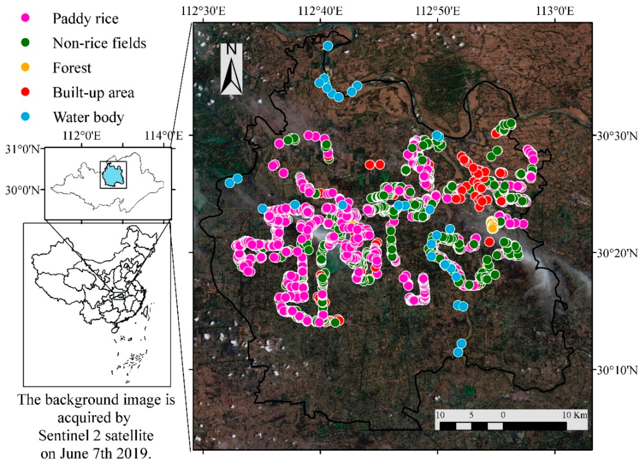
2.1. Study Area

The study area, shown in Figure 1, is the Qianjiang region in Hubei Province, which is about 2000 km². The Qianjiang region is located on Jianghan Plain, one of the most important plains of the Yangtze Plain [35], near the Yangtze River and Han River. Qianjiang region is a flat, water-land crisscrossed landscape that is interconnected by waterways and dotted lakes. The elevation of the Qianjiang region is only about 26–31 m, which makes the whole area plain. The surface texture mainly comprises of modern river alluvial and lake silt, such as fine sand, silt, and clay. The subtropical monsoon climate brings ample sunlight and warms the region during rainy season. The annual average precipitation is around 1300 mm. The rain and heat are synchronous in Jianghan Plain, which is the typical sub-tropical monsoon climate. Furthermore, most of the extreme precipitation events (more than 90%) occur during the rainy season between May and October, and more than 30% of these extreme events concentrate in July [36]. Therefore, during the paddy rice growth period, cloud contamination could be a very serious problem.

All these conditions are highly conducive to paddy rice production, making the Qianjiang region as one of the important commodity grain production bases in China. The total rice production is more than 70% of Hubei Province. The total area of paddy field is more than 50% of the total paddy fields in Hubei Province [37].

The middle-season rice is a dominating type of paddy rice, while other types, including early, and late rice, also have a notable presence. Therefore, the study period is from March to September, encompassing all the stages of each of the different kinds of paddy rice. The production method on Jianghan Plain is primarily smallholder agricultural production, and the area of paddy is generally small. As mentioned, the spatial resolution of Sentinel-2 (10 m and 20 m) is considered suitable for the study. On Jianghan Plain, other main crop species, including rape, cotton, wormwood, lotus root, grass, other vegetables, wetland vegetation, and corn, are considered as alternate crops against paddy rice.

2.2. Datasets and Pre-Processing

2.2.1. Sentinel Data

The optical datasets used are Sentinel-2 multispectral imager (MSI) Level-2A images. The microwave SAR datasets are Sentinel-1 SAR ground range detected (GRD): C-band synthetic aperture radar ground range detected, log scaling images. Both datasets are selected from March to September 2019, including all the months that all kinds of rice exist. Sentinel satellites provide high spatial and temporal resolution products which have been successfully applied to estimating canopy chlorophyll and nitrogen (N) content [38], soil moisture retrieving [39], vegetation classification [40] and land cover classification [41].

The SAR data collection mode used in this study was interferometric wide swath (IW) out of four modes Stripmap (SM), interferometric wide swath (IW), extra wide swath (EW) and wave (WV). IW mode is the primary operational mode over land, preserving revisit performance with consistent long-term archives. The SAR imagery used in this study was received from a dual-polarization C-band Synthetic Aperture Radar (SAR) instrument with vertical transmit, vertical receive (VV), and vertical transmit, horizontal receive (VH).

Level-1 ground range detected (GRD) product is a calibrated, ortho-corrected product. Google Earth Engine (GEE) has pre-processed the Sentinel-1 data to derive the backscatter coefficient in each pixel as implemented by the Sentinel-1 toolbox. Because thermal noise still has to be removed to enhance the quality of the detected images, a simple noise filter calculating the average value of the circle with a radius of 7 pixels is applied to the images. The L2A level products are processed by Sen2Cor, which performs the atmospheric, terrain and cirrus correction of top-of-atmosphere Level 1C input data. Sen2Cor creates bottom-of-atmosphere corrected reflectance after the radiometric calibration and atmospheric correction, which means that the image pre-processing still has to remove the cloud. In this study, we have selected images with less than 20% of cloud coverage.

After the cloud selection, the number of optical images is less than the SAR images in the same period. Therefore, the time to generate one image for optical is longer. The optical images were reduced to one image using Maximum Value Composite, by calculating the maximum vegetation index value of each pixel during one month. SAR images were reduced to one image by calculating the minimum value of each pixel across the stack of all matching bands in a period of two weeks. Because of plum rain, there are no available images that satisfy the needs in July due to cloud coverage. As a result, the optical image datasets only contain six images to calculate the corresponding vegetation indices. The information about GEE derived SAR and optical data used for the study is shown in

Table 1. The characteristics of the GEE derived SAR and optical data used for the study.

Datasets	Optical Datasets	Microwave SAR Datasets
Source	Sentinel-2 MSI, Level-2A images	Sentinel-1 SAR GRD
Time span	March to September 2019	March to September 2019
Spatial resolution	10–20 m	10 m
Pre-processing	Cloud coverage < 20%	Speckle filter
Composition	Maximum Value Composite during one month	The minimum value of each pixel in a period of two weeks

.

2.2.2. Field Samples

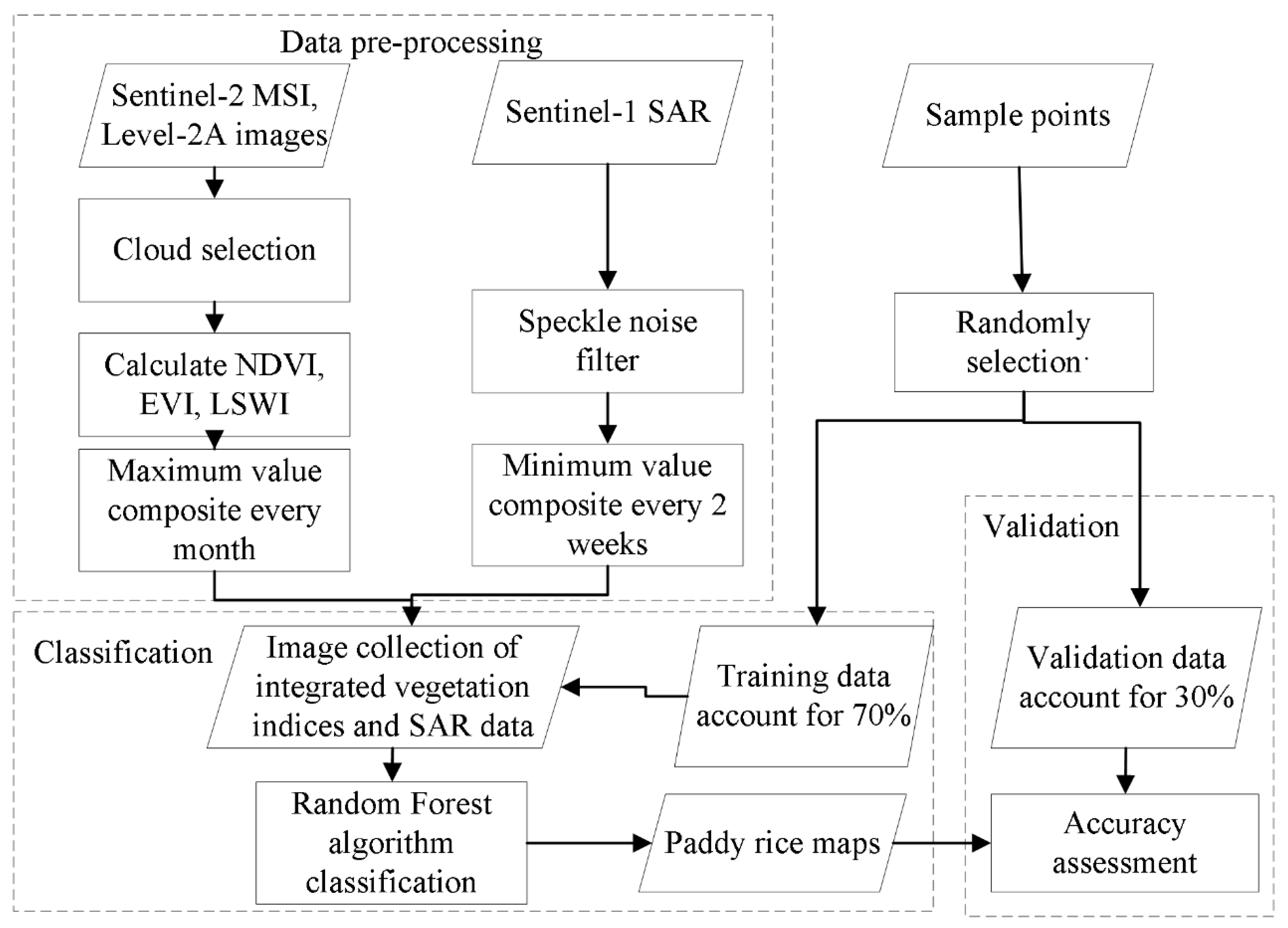
To ensure the accuracy of training and validation data, we collected around 2000 points, across 19 types of field samples in a ground survey in 2019. We divided the land type into five border types: (1) paddy rice (2) non-rice fields, including rapeseed, cotton, wormwood, lotus, grass, wetland vegetation, corn, and other vegetables, (3) forest, (4) built-up area, and (5) water body, as shown in

Table 2. Field survey data class and border type.

Border Type	Name	Description
1	Paddy rice	Early rice (double cropping rice or ratoon rice), middle rice (single-season rice or middle-late rice, mainly single-season rice), crayfish paddy rice, ratoon rice
2	Non-rice fields	Rape, cotton, wormwood, lotus, grass, wetland vegetation, corn, other vegetables
3	Forest	Orchard, evergreen broad-leaf forest, broadleaved deciduous forest, coniferous forest, shrub
4	Built-up area	Greenhouse
5	Water body	Lake, river, and pond

. Table 2 describes five border class and their dominated objects in each class to provide a clear understanding of paddy rice and other land covers in this typical study area. In addition to the ground survey data, sample points for forest, built-up area, and water body were manually selected from Google Earth to complement the training and validation data. Based on the sample dataset mentioned above, 1508 points were randomly selected for the training and validation. The selected set of sample data was randomly split into 70/30 percent separately for training and classification accuracy assessment, respectively.

2.2.3. Methodology

As shown in Figure 2, in this study, Sentinel-2 images are pre-processed through cloud selection and composition. Then we used the processed images to calculate multiple vegetation indices (NDVI, EVI, LSWI). Sentinel-1 SAR data is processed through speckle-noise filter and composition. These two datasets are integrated together. All these procedures are processed on Google Earth Engine. The details of this method are presented ahead.

Firstly, a different combination of multi-temporal polarization bands and vegetation indices derived from optical bands were used for the paddy rice classification experiments. The polarization method is VV and VH; and the vegetation indices are NDVI, LSWI, and EVI. Thus, there are five variables in the experiment. A total of 39 experiments were performed to evaluate how exactly the various combinations of different variables influence the results. After pre-processing, three vegetation indices, namely NDVI, EVI, and LSWI, were calculated for each image as follows:

$$\mathrm{NDVI}=\frac{\mathrm{NIR}-\mathrm{RED}}{\mathrm{NIR}+\mathrm{RED}}$$

(1)

$$\mathrm{EVI}=2.5\ast \frac{\mathrm{NIR}-\mathrm{RED}}{\mathrm{NIR}+6\times \mathrm{RED}-7.5\times \mathrm{BLUE}+1}$$

(2)

$$\mathrm{LSWI}=\frac{\mathrm{NIR}-\mathrm{SWIR}}{\mathrm{NIR}+\mathrm{SWIR}}$$

(3)

As the assets contain 12 UINT16 spectral bands representing SR (spectral reflectance) scaled by 10000, NDVI, EVI, and LSWI of Sentinel images were calculated with GEE as follows:

$$\mathrm{NDVI}=\frac{\mathrm{B}8-\mathrm{B}4}{\mathrm{B}8+\mathrm{B}4}$$

(4)

$$\mathrm{EVI}=2.5\ast \frac{\mathrm{B}8-\mathrm{B}4}{\mathrm{B}8+6\times \mathrm{B}4-7.5\times \mathrm{B}2+10000}$$

(5)

$$\mathrm{LSWI}=\frac{\mathrm{B}8\mathrm{A}-\mathrm{B}11}{\mathrm{B}8\mathrm{A}+\mathrm{B}11}$$

(6)

The accuracy assessment is presented through a confusion matrix. Other accuracy indices to assess the performance of the classification includes overall classification accuracy, producer’s accuracy, user’s accuracy, and Kappa statistic.

There are many examples using machine learning to classify crop, including neutral network [42], decision tree algorithms [43], support vector machines [44,45,46], and random forest algorithm [47,48,49]. Among these algorithms, the random forest is proven to be an accurate classification algorithm to handle large and diverse datasets [50]. The random forest algorithm is used in the study [51]. This algorithm is based on the classification and decision tree, which has been successfully applied for many study areas in remote sensing [52]. The random forest algorithm is based on a collection of decision trees. Each tree uses a subset of training data by bagging, and the best split variable is used to split the nodes, leaving the remaining data points for internal cross-validation.

As for the platform used in the study, Google Earth Engine is a cloud platform hosting a multi-petabyte catalog of satellite imagery and geospatial datasets with planetary-scale analysis capabilities. Using GEE helps in reducing the pre-processing and data downloading steps, which would otherwise require high data storage capacity and intense computational power. The method proposed in this study requires multi-temporal images for several months. On Google Earth Engine, multi-petabyte datasets are easily accessed and mostly pre-processed. Secondly, the high-performance computing resources allows users to apply a machine-learning algorithm to get the validated result. The image collection of integrated vegetation indices and SAR data is used as the basis to train the random forest algorithm to classify the paddy rice. Finally, the extracted paddy rice classification map was validated by 30% sample points randomly selected early. The variable importance is calculated through the “.explain()” method on Google Earth Engine.

3. Result

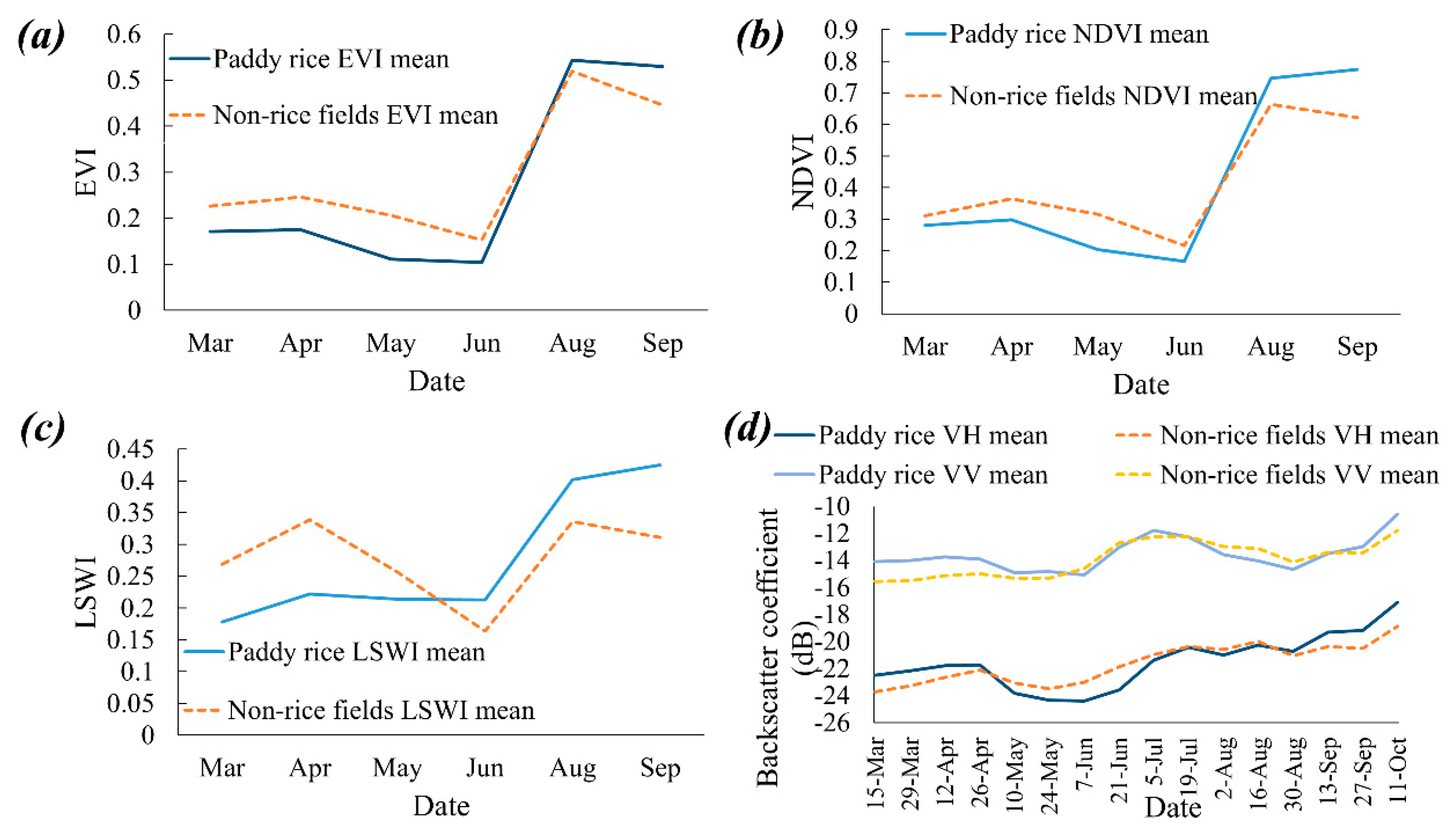
3.1. NDVI, LSWI, and EVI Results

Figure 3 shows the temporal profiles of the mean values of vegetation indices (EVI, NDVI, LSWI) and polarization band for the paddy rice and non-rice fields over the study area in 2019. In this study area, the type of paddy rice includes several types, and hence the temporal profile is not reflective of one phenological change but the broader tendency of paddy rice in the study area.

Figure 3 shows that the paddy rice and non-rice fields has a similar trend in general. However, using these three vegetation indices could still separate one type from the other in the end by using this method. The general trend is that all three indices rises up during the period. At the beginning paddy rice’s indices are lower. A turning point appears around June making paddy rice’s value larger than non-rice’s of all three indices. Before June, 0.2 is larger than paddy rice’s value, while lower than non-rice’s EVI. In respect of NDVI, 0.3 could be the threshold before June. As for LSWI, both types of paddy rice and non-rice are rising at first. But still before June paddy rice’s LSWI is lower. After July, paddy rice’s indices all exceed non-rice fields. Paddy rice’s NDVI is larger than 0.7 while non-rice’s lower. And 0.4 could be the threshold for LSWI.

In addition to the assessment of the temporal profiles of vegetation indices for the six months period, we added SAR data to improve the classification accuracy. As for polarization band for the paddy rice and non-rice fields, it also shows a rising general trend for both VV and VH band. The backscatter coefficient depends on variables such as surface roughness, soil moisture, and texture. At the beginning, both VV and VH have a higher value for paddy rice than non-rice fields. The reason of why the paddy rice’s VH is lower during May and June could be the majority of paddy is during transplanting at that time. The water gives a low backscatter coefficient. After tillering, leaves and stem grow up, covering the water, rising the backscatter coefficient. Around September, most of the paddy rice is mature. The backscatter coefficient exceeds other non-paddy rice fields.

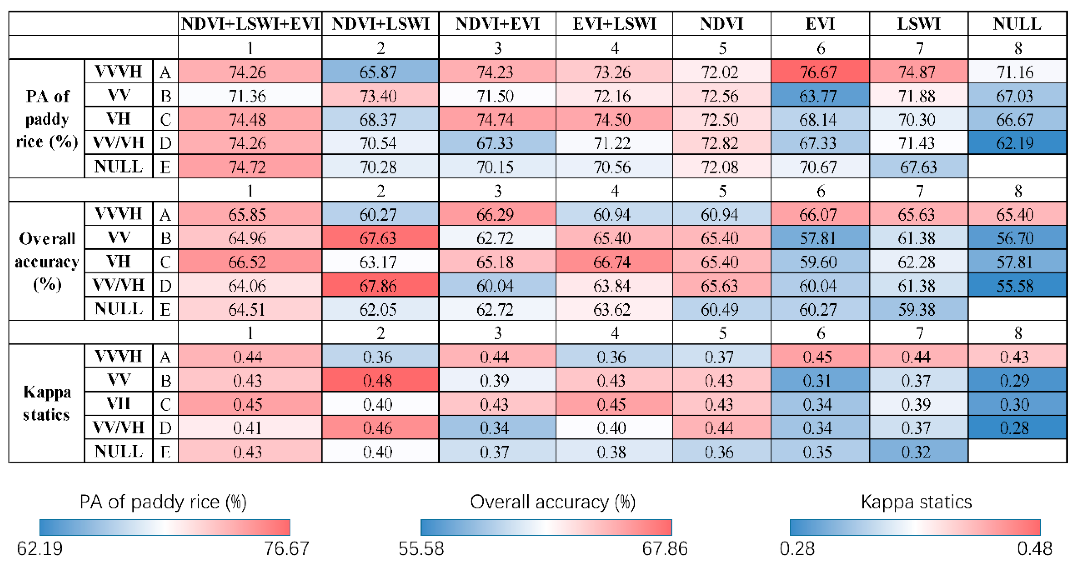
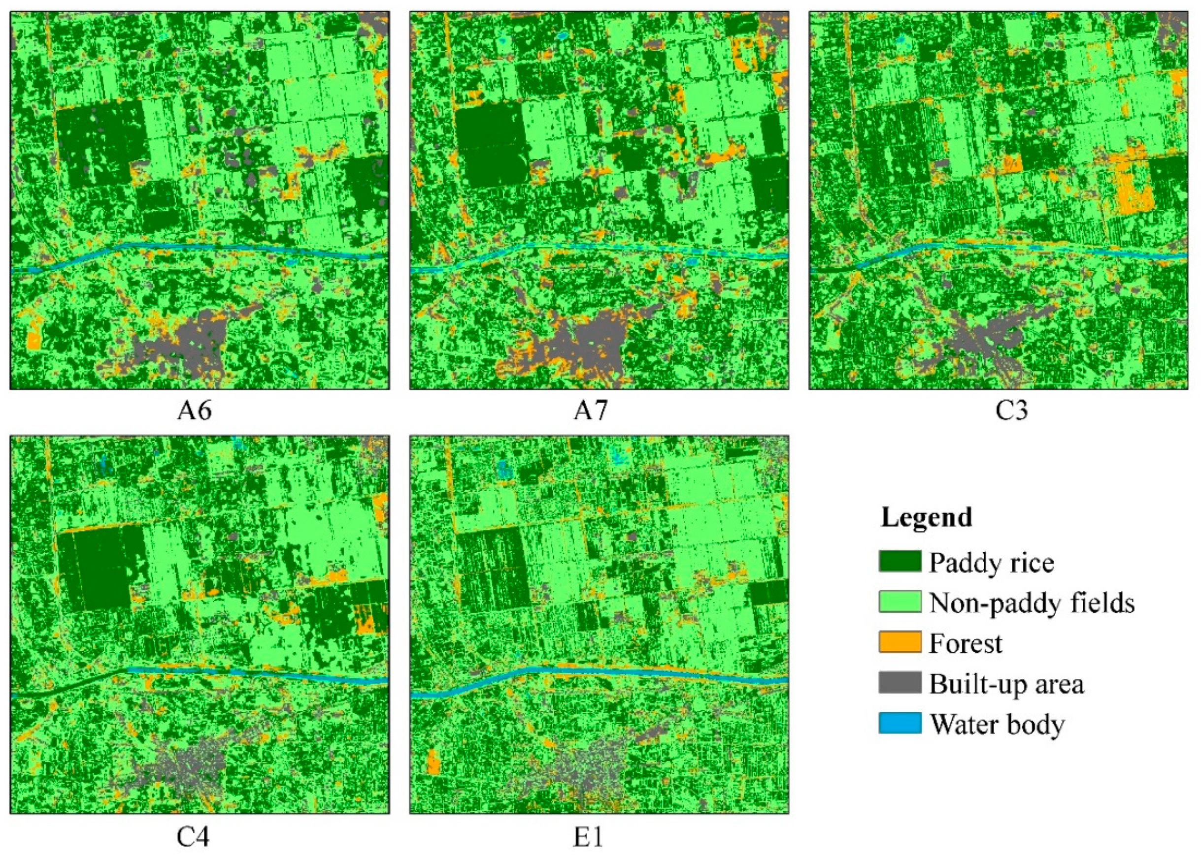
3.2. Paddy Rice Mapping Results

This section summarizes the results of 39 classification experiments.

Table 3. Combination of the dataset used in this study.

Vegetation Indices Combination		Polarization Band Combination
CODE	Combination	CODE	Combination
1	NDVI + LSWI + EVI	A	VVVH
2	NDVI + LSWI	B	VV
3	NDVI + EVI	C	VH
4	EVI + LSWI	D	VV/VH
5	NDVI	E	null
6	EVI
7	LSWI
8	null

codifies the different input datasets. In the table, A through E refers to the various combinations of polarization bands, while 1–8 refers to the combinations of different vegetation indices. For instance, B7 stands for the combination of VV bands and LSWI.

Overall experiment results, including the producer accuracy (PA), overall accuracy, and Kappa statistics of each experiment, are presented in Figure 4. A number of combinations provide high accuracy results, which are analysed in further detail, as shown in Figure 5. For the sample points, we randomly selected 70% for the training algorithm to produce the paddy rice map. The other 30% are used for accuracy assessment.

The best combination for mapping paddy rice fields emerges as A6 with EVI and VV and VH band; the producer’s accuracy of paddy rice (PA) was 76.67%, with the overall accuracy (OA) of 66.07%, and Kappa statistics of 0.45. Generally, more variables used for the combination trends to have a better accuracy generally, for both vegetation indices and polarization bands.

The highest results in each column or row is considered as the “best” performance. Counting the number of the “best” performance could evaluate the principle of the combination of polarization band under the same condition of vegetation indices, and vice versa. For similar vegetation indices, generally, the VV yielded one “best” performances B2, while VH band yielded two, C3 and C4. The combination of VV and VH bands has three “best” performance, A6, A7, A8. The VV/VH band combinations have D5 only. However, when no polarization band is used, vegetation indices had one “best” performances, E1. From these results, the VV and VH band combinations showed better performance, and the other polarization band combinations did not provide encouraging results.

For the same polarization band, the contribution of each vegetation indices was considered next. In row A, using the combination of VV and VH, the best performance was noted for the experiment adding EVI, which is also the overall “best” out of all experiments. Using only the VV/VH, the “best” performance was with the combination of three vegetation indices, D1. Only using VV, the “best” performance were B2, with PA, OA, and Kappa values as 73.4%, 67.63%, and 0.48, respectively. Only using VH, the “best” performance were C3, with PA, OA, and Kappa values as 74.74%, 65.18%, and 0.43, respectively. The best result of the experiment using only vegetation indices was the experiment using three indices, E1, with PA of paddy rice as 74.72%, OA as 64.51%, and Kappa value of 0.43. Thus, on the whole, no index or combination show encouraging results significantly.

To analyse the different results of “top performers”, we selected top 5 experiments for the paddy rice’s PA, which is greater than 74.49%. Figure 5 presents a closer view for A6 (VV + VH + EVI), A7 (VV + VH + LSWI), C3 (VH + NDVI + EVI), C4 (VH + EVI + LSWI), and E1 (NDVI + EVI + LSWI).

Results from E1 are highly fragmentized, indicating that the integration of polarization bands could increase not only the classification accuracy but also benefit the morphology of the extraction map. This made the shape of the classification result fit the real surface feature better. The other four results with polarization bands clearly show a better visualization. In contrast, A6 and A7 do not present the actual shape of crop fields. For water bodies, E1 also shows a relatively better performance. C3 shows a good texture of crop fields and urban area. The A6 combination shows relatively best performance considering the producer’s accuracy, and C3 have a better visualization. In particular, C3 can demarcate the quadrilateral shape of cropland and the precise shape of the urban area. The relationship between accuracy and morphology needs further study in the future.

The spatial distribution of classification error in these six experiments are shown in Figure 6 and discussed in more detail ahead in Section 4.2. Several reasons could cause a classification error. For example, crop rotation could cause the temporal field to be different. Even though the same type of paddy rice was planted, different crops planted before or after could disturb the classification result. The mixed cropping also creates a difference in the same type of crop. Whether these combinations could be applied to other areas with similar accuracy needs further testing and can be undertaken in a future study.

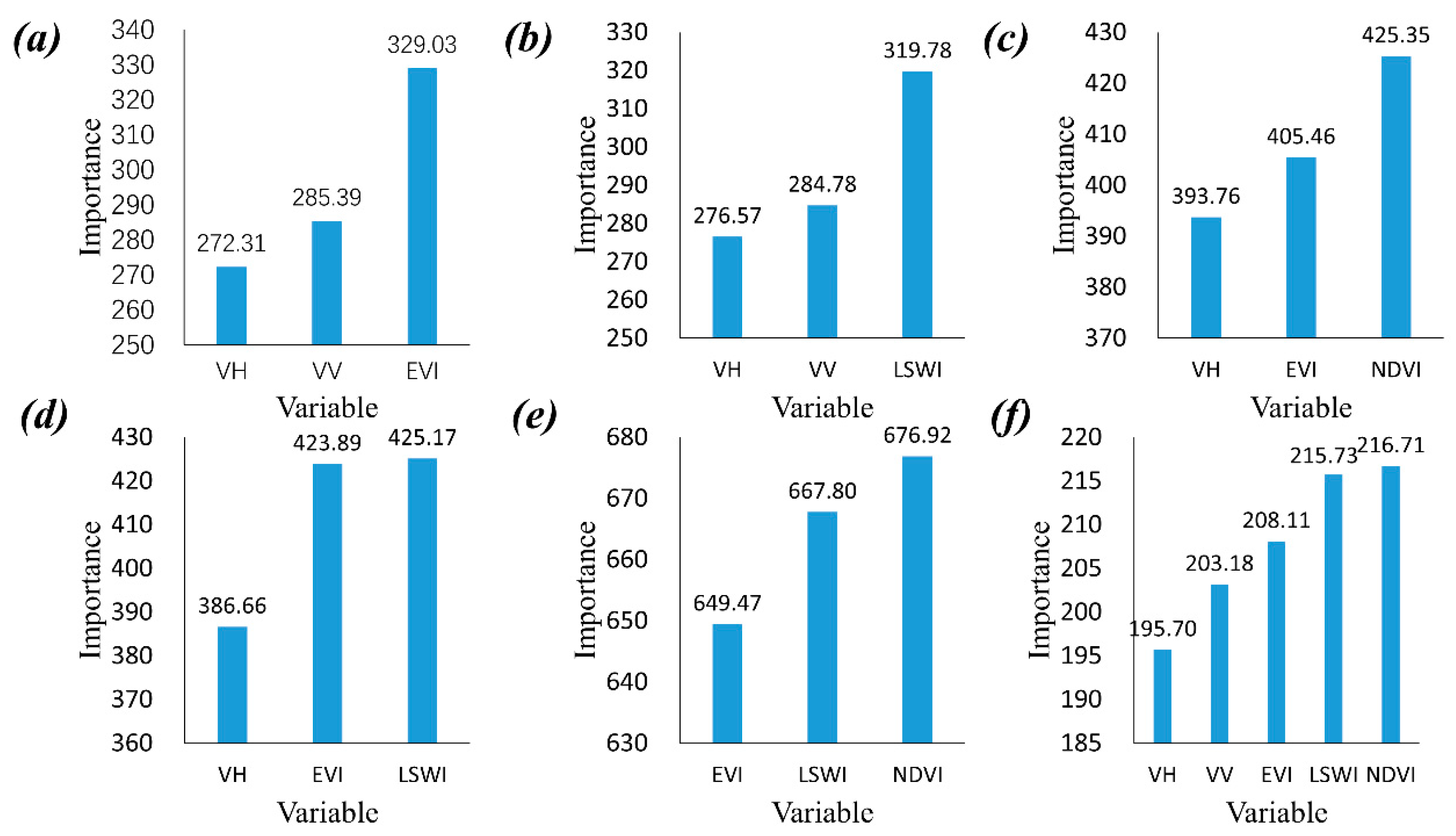
3.3. Variable Importance Results

To analyse the variables importance, we selected top five experiments for the paddy rice’s PA and one experiment with all five variables. As shown in Figure 7, in general, we can see the trend that the order of variable importance is NDVI, LSWI, EVI, VV, VH. One study believes that the VH signal could better represent the actual rice-growth cycle [53]. However, the variable importance result in this study shows that VV contributes more than VH in the classification.

4. Discussions

4.1. Classification Improvement by Integrating SAR Data

This study reviewed the performance of using a different combination of vegetation indices and polarization bands to extract the paddy rice. Some studies [54] have found that the integrated polarization SAR bands with NDVI could improve the overall classification accuracy. Based on the prior findings, this study selected three vegetation indices (NDVI, EVI, LSWI) to represent the phenological evolution, and used SAR imagery as a supplement to separate paddy fields from adjoining crop fields.

The optical vegetation indices dataset employed in this study is comprised of six images in March, April, May, June, August, and September, i.e., covering six months in 2019. July is missing because of the plum rain. In addition to multi-temporal optical vegetation indices, the SAR dataset is integrated with phenological information to provide a more accurate description. Each type of paddy rice was not classified separately, and the study duration is sufficiently long to include all the paddy rice types in the study area. The different performance of different combinations of variables was reviewed. The results indicate that the combination of VV and VH and EVI band could produce a convincing classification result (paddy rice PA is 76.67%).

The confusion tables of the combination of VV and VH and EVI with or without the polarization band in July are presented in

Table 4. Confusion table of the combination of VV and VH and EVI.

	Estimated Classification	Paddy Rice	Non-Rice Fields	Forest	Built-Up Area	Water Body	User’s Accuracy
Observed Classification
Paddy rice		138	73	0	5	2	63%
Non-rice fields		40	121	3	6	4	70%
Forest		0	5	8	1	0	57%
Built-up area		1	10	1	22	0	65%
Water body		1	0	0	0	7	88%
Producer’s accuracy (PA)		77%	58%	67%	65%	54%

and

Table 5. Confusion table of the combination of VV and VH and EVI without VV and VH bands in July.

	Estimated Classification	Paddy Rice	Non-Rice Fields	Forest	Built-Up Area	Water Body	User’s Accuracy
Observed Classification
Paddy rice		144	65	2	4	3	66%
Non-rice fields		64	90	8	4	8	52%
Forest		0	5	8	1	0	57%
Built-up area		1	6	10	17	0	50%
Water body		2	1	0	0	5	63%
Producer’s accuracy (PA)		68%	54%	29%	65%	31%

, respectively. By comparison, we can see that the paddy rice PA increases from 68% to 77% after adding the polarization band. It appears that adding a polarization band could increase the accuracy of paddy rice extraction when vegetation indices are unavailable. The backscattering coefficient could reflect the texture of the surface feature. So, the difference surface during the vegetation grows could be captured. Moreover, the synthetic aperture radar data penetrating the clouds could monitor the ground all time to fill the phenological phenomenon missed in optical remote sensing data.

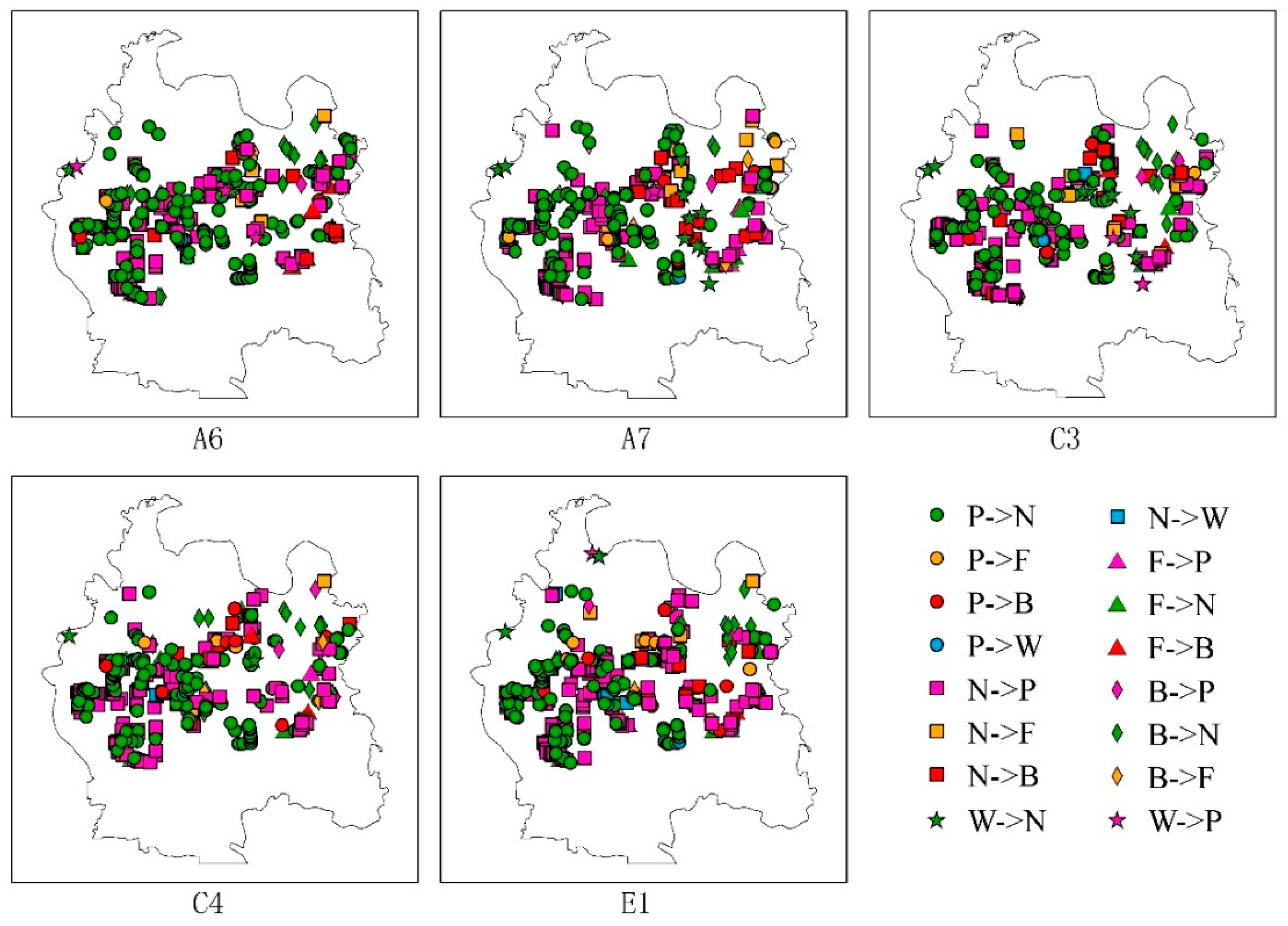
4.2. Error Analysis for Different Data Combinations

Figure 6 presents the spatial distribution of the classification error of five experiments for paddy rice’s PA higher than 74.49%. The legend used in Figure 6 uses the same shape for the same true type and the same colour for the same classified type. For instance, no matter what the pixel type is classified as, if the field sample finds it is paddy rice, it is represented by a circle on the map. Also, no matter what type the true type is, if it is classified as non-paddy field, then the pixel is shown as green on the map.

As a whole, it is found that the error of paddy and non-paddy is more than other types. Green is the domain colour on all maps. Generally, the error is concentrated in the southwest of the study area, as the city area of Qianjiang City is in the northeast, which makes the crop fields are mainly at the south and the west. So, the misclassification between paddy rice fields and non-paddy rice fields are concentrated in the southwest. Further, in the northeast, there are more type of misclassification error. Between paddy rice fields and non-paddy rice fields, the shape of the field or the spatial distribution do not have a pattern, which means in this study area the paddy rice and other crop equally planted and it is difficult to differentiate them from certain optical images. Thus, temporal profile, which the combination of optical vegetation index and SAR could necessarily contribute to build, is essential to classification,

In all five experiments, the actual paddy rice classified as non-paddy by error is more than the other way around. A6, with the highest PA, also has the highest difference between misclassified paddy field and misclassified non-paddy fields. C3 has the most even number in two misclassified types. Compared to other combinations, C4 appears to be more concentrated on a specific type. The classification error could be caused by crop rotation and the mixed cropping. Moreover, whether these combinations could be applied to other areas with similar accuracy needs further testing and can be undertaken in a future study.

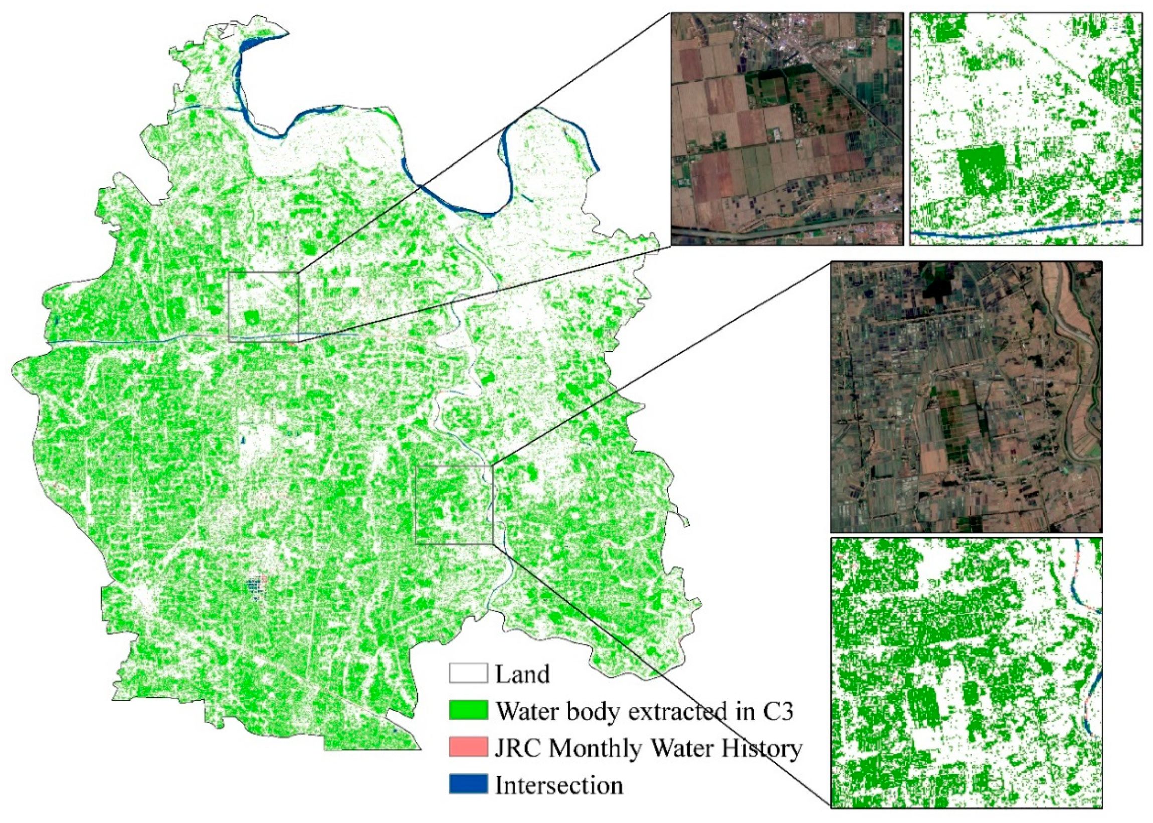
4.3. Comparison with a Current Water Body Product

To evaluate how much this study could improve water body extraction. We compared our result from C3 (VH + NDVI + EVI) with The European Commission’s Joint Research Centre (JRC) Monthly Water History [4] in 2019 September. JRC Monthly Water History displays water surfaces that are visible from space, including natural (rivers, lakes, coastal margins and wetlands) and artificial water bodies (reservoirs formed by dams, flooded areas such as opencast mines and quarries, flood irrigation areas such as paddy fields, and water bodies created by hydro-engineering projects such as waterway and harbor construction) between March 1984 and October 2015 on a month-by-month basis. This dataset contains maps of the location and temporal distribution of surface water and provides statistics on the extent and change of the water surfaces. However, there is still a lot of omission of water body caused by paddy rice fields for its short duration, small size, or crop cover. As the most important artificial water body, paddy rice fields are highly fractured, especially in South China. The accuracy of water extraction would rise as the paddy rice fields are extracted correctly. Hence, this study could improve the paddy rice extraction and fill the missing area dramatically.

Figure 8 shows that both C3 and JRC could successfully extract the main river area. Around the permanent rivers and lakes, the extracted water body are almost the same in JRC and C3. Nevertheless, as for paddy rice, JRC, surprisingly, does not show any water area, while C3 mapped the paddy rice fields in the study area. The JRC and C3 have 21,782 pixels overlap. While JRC Monthly Water History has 10,889 pixels that C3 is missing as a water body, C3 has extracted 949,741 pixels that have not been mapped as a water body in the JRC data. This indicates that the approach outlined in this study could substantially improve the water body extraction, especially around the paddy fields, by identifying the artificial wetland that was found to be missing.

5. Conclusions

This study has demonstrated the combination of optical vegetation index, and SAR imagery can effectively extract the paddy rice area, overcoming the month-long cloud impacted data in the cloud-prone area, e.g., Jianghan Plain. A multi-temporal dataset from Sentinel is processed on GEE using a random forest algorithm. The temporal profiles show that the three vegetation indices still could differentiate paddy rice from non-paddy fields. All three indices rise during the period. At the beginning, paddy rice’s indices are lower. A turning point appears around June making paddy rice’s value larger than non-rice’s of all three indices. After July, paddy rice’s indices all exceed non-rice fields. As for the polarization band for the paddy rice and non-rice fields, it also shows a rising general trend for both VV and VH band. However, the specific contribution of VV and VH band separately is remain uncovered.

Generally, more variables used for the combination trends to have a better accuracy generally, for both vegetation indices and polarization bands. The classification results present that the best combination is EVI and VV and VH polarization band accuracy. The VH + NDVI + EVI shows the best performance in morphology. As for variable importance, in general, we can see the trend that the order of variable importance is NDVI, LSWI, EVI, VV, VH.

The study result has shown that paddy rice PA increases from 68% to 77% after adding the polarization band, which demonstrates that adding a polarization band could increase the accuracy of paddy rice extraction when vegetation indices are unavailable. Most of the paddy rice grows in the monsoon region, where there have strong rain fall and cloud during the paddy rice growth period. This could cause serious problem to paddy rice extraction by lacking the useful optical images. Therefore, the synthetic aperture radar data penetrating the clouds could fill the phenological phenomenon missed in optical remote sensing data, so as to improve the accuracy of paddy rice extraction.

By extracting the accuracy area and distribution of paddy rice, the water body area could be filled dramatically. As the most important artificial water body, highly fractured and temporal paddy rice fields have always been the difficulty in this study field. As a consequence, this study could contribute to the food security and water use assessments.

Although the method could extract paddy rice as one type, the accuracy still has room for improvements. In addition to the NDVI, EVI, and LSWI, other vegetation indices could also have an impact on the classification result. The next step resulting from this study would be to explore other variables to improve classification accuracy. Furthermore, the results of using the proposed approach in other areas still need to be tested.

References

1. Maclean, J.L.; Dawe, D.C.; Hardy, B.; Hettel, G.P. Rice Almanac: Source Book for the Most Important Economic Activity on Earth; Int. Rice Res. Inst.: Los Baños, Philippines, 2002. [Google Scholar]
2. Bouman, B. How much water does rice use? Rice Today 2009, 8, 28–29. [Google Scholar]
3. Chen, Z.; Ren, J.; Tang, H.; Shi, Y.; Liu, J. Progress and perspectives on agricultural remote sensing research and applications in China. J. Remote Sens. 2016, 20, 748–767. [Google Scholar] [CrossRef]
4. Pekel, J.F.; Cottam, A.; Gorelick, N.; Belward, A.S. High-resolution mapping of global surface water and its long-term changes. Nature 2016, 540, 418–422. [Google Scholar] [CrossRef] [PubMed]
5. Xiao, X.; Boles, S.; Liu, J.; Zhuang, D.; Frolking, S.; Li, C.; Salas, W.; Moore, B. Mapping paddy rice agriculture in southern China using multi-temporal MODIS images. Remote Sens. Environ. 2005, 95, 480–492. [Google Scholar] [CrossRef]
6. Gumma, M.K.; Nelson, A.; Thenkabail, P.S.; Singh, A.N. Mapping rice areas of South Asia using MODIS multitemporal data. J. Appl. Remote Sens. 2011, 5, 1–27. [Google Scholar] [CrossRef] [Green Version]
7. Qiu, B.; Li, W.; Tang, Z.; Chen, C.; Qi, W. Mapping paddy rice areas based on vegetation phenology and surface moisture conditions. Ecol. Indic. 2015, 56, 79–86. [Google Scholar] [CrossRef]
8. Friedl, M.A.; McIver, D.K.; Hodges, J.C.; Zhang, X.Y.; Muchoney, D.; Strahler, A.H.; Woodcock, C.E.; Gopal, S.; Schneider, A.; Cooper, A.; et al. Global land cover mapping from MODIS: Algorithms and early results. Remote Sens. Environ. 2002, 83, 287–302. [Google Scholar] [CrossRef]
9. Bicheron, P.; Defourny, P.; Brockmann, C.; Schouten, L.; Vancutsem, C.; Huc, M.; Bontemps, S.; Leroy, M.; Achard, F.; Herold, M.; et al. GLOBCOVER: Products Description and Validation Report. 2008. Available online: http://due.esrin.esa.int/page_globcover.php (accessed on 29 July 2020).
10. Frolking, S.; Qiu, J.; Boles, S.; Xiao, X.; Liu, J.; Zhuang, Y.; Li, C.; Qin, X. Combining remote sensing and ground census data to develop new maps of the distribution of rice agriculture in China. Glob. Biogeochem. Cycles 2002, 16, 38-1. [Google Scholar] [CrossRef] [Green Version]
11. Monfreda, C.; Ramankutty, N.; Foley, J.A. Farming the planet: 2. Geographic distribution of crop areas, yields, physiological types, and net primary production in the year 2000. Glob. Biogeochem. Cycles 2008, 22. [Google Scholar] [CrossRef]
12. McCloy, K.R.; Smith, F.R.; Robinson, M.R. Monitoring rice areas using LANDSAT MSS data. Int. J. Remote Sens. 1987, 8, 741–749. [Google Scholar] [CrossRef]
13. Rao, P.P.N.; Rao, V.R. Rice crop identification and area estimation using remotely-sensed data from Indian cropping patterns. Int. J. Remote Sens. 1987, 8, 639–650. [Google Scholar] [CrossRef]
14. Fang, H. Rice crop area estimation of an administrative division in China using remote sensing data. Int. J. Remote Sens. 1998, 19, 3411–3419. [Google Scholar] [CrossRef]
15. Oguro, Y.; Suga, Y.; Takeuchi, S.; Ogawa, M.; Konishi, T.; Tsuchiya, K. Comparison of SAR and optical sensor data for monitoring of rice plant around Hiroshima. Adv. Space Res. 2001, 28, 195–200. [Google Scholar] [CrossRef]
16. Pan, X.-Z.; Uchida, S.; Liang, Y.; Hirano, A.; Sun, B. Discriminating different landuse types by using multitemporal NDXI in a rice planting area. Int. J. Remote Sens. 2010, 31, 585–596. [Google Scholar] [CrossRef]
17. Nguyen, T.T.H.; De Bie, C.A.J.M.; Ali, A.; Smaling, E.M.A.; Chu, T.H. Mapping the irrigated rice cropping patterns of the Mekong delta, Vietnam, through hyper-temporal SPOT NDVI image analysis. Int. J. Remote Sens. 2012, 33, 415–434. [Google Scholar] [CrossRef]
18. Xiao, X.; Boles, S.; Frolking, S.; Salas, W.; Moore, B.; Li, C.; He, L.; Zhao, R. Observation of flooding and rice transplanting of paddy rice fields at the site to landscape scales in China using VEGETATION sensor data. Int. J. Remote Sens. 2002, 23, 3009–3022. [Google Scholar] [CrossRef]
19. Sakamoto, T.; van Phung, C.; Kotera, A.; Nguyen, K.D.; Yokozawa, M. Analysis of rapid expansion of inland aquaculture and triple rice-cropping areas in a coastal area of the Vietnamese Mekong Delta using MODIS time-series imagery. Landsc. Urban Plan. 2009, 92, 34–46. [Google Scholar] [CrossRef]
20. Sun, H.-S.; Huang, J.-F.; Huete, A.R.; Peng, D.-L.; Zhang, F. Mapping paddy rice with multi-date moderate-resolution imaging spectroradiometer (MODIS) data in China. J. Zhejiang Univ.-Sci. A 2009, 10, 1509–1522. [Google Scholar] [CrossRef]
21. Torbick, N.; Salas, W.A.; Hagen, S.; Xiao, X. Monitoring Rice Agriculture in the Sacramento Valley, USA with Multitemporal PALSAR and MODIS Imagery. IEEE J. Sel. Top. Appl. Earth Obs. Remote Sens. 2011, 4, 451–457. [Google Scholar] [CrossRef]
22. Dong, J.; Xiao, X. Evolution of regional to global paddy rice mapping methods: A review. ISPRS J. Photogram. Remote Sens. 2016, 119, 214–227. [Google Scholar] [CrossRef] [Green Version]
23. Bridhikitti, A.; Overcamp, T.J. Estimation of Southeast Asian rice paddy areas with different ecosystems from moderate-resolution satellite imagery. Agric. Ecosyst. Environ. 2012, 146, 113–120. [Google Scholar] [CrossRef]
24. Yang, S.; Shen, S.; Li, B.; Toan, T.L.; He, W. Rice Mapping and Monitoring Using ENVISAT ASAR Data. IEEE Geosci. Remote Sens. Lett. 2008, 5, 108–112. [Google Scholar] [CrossRef]
25. Bouvet, A.; le Toan, T. Use of ENVISAT/ASAR wide-swath data for timely rice fields mapping in the Mekong River Delta. Remote Sens. Environ. 2011, 115, 1090–1101. [Google Scholar] [CrossRef] [Green Version]
26. Li, K.; Brisco, B.; Yun, S.; Touzi, R. Polarimetric decomposition with RADARSAT-2 for rice mapping and monitoring. Can. J. Remote Sens. 2012, 38, 169–179. [Google Scholar] [CrossRef]
27. Nelson, A.; Setiyono, T.; Rala, A.B.; Quicho, E.D.; Ninh, N.H. Towards an Operational SAR-Based Rice Monitoring System in Asia: Examples from 13 Demonstration Sites across Asia in the RIICE Project. Remote Sens. 2014, 6, 94–105. [Google Scholar] [CrossRef] [Green Version]
28. Singha, M.; Dong, J.; Zhang, G.; Xiao, X. High resolution paddy rice maps in cloud-prone Bangladesh and Northeast India using Sentinel-1 data. Sci. Data 2019, 6, 26. [Google Scholar] [CrossRef]
29. Onojeghuo, A.O.; Blackburn, G.A.; Wang, Q.; Atkinson, P.M.; Kindred, D.; Miao, Y. Mapping paddy rice fields by applying machine learning algorithms to multi-temporal sentinel-1Aand landsat data. Int. J. Remote Sens. 2018, 39, 1042–1067. [Google Scholar] [CrossRef] [Green Version]
30. Jat, P.; Serre, M.L. A novel geostatistical approach combining Euclidean and gradual-flow covariance models to estimate fecal coliform along the Haw and Deep rivers in North Carolina. Stoch. Environ. Res. Risk Assess 2018, 32, 2537–2549. [Google Scholar] [CrossRef]
31. Liu, X.; Zhai, H.; Shen, Y.; Lou, B.; Jiang, C.; Li, T.; Hussain, S.B.; Shen, G. Large-Scale Crop Mapping From Multisource Remote Sensing Images in Google Earth Engine. IEEE J. Sel. Top. Appl. Earth Obs. Remote Sens. 2020, 13, 414–427. [Google Scholar] [CrossRef]
32. Gorelick, N.; Hancher, M.; Dixon, M.; Ilyushchenko, S.; Thau, D.; Moore, R. Google Earth Engine: Planetary-scale geospatial analysis for everyone. Remote Sens. Environ. 2017, 202, 18–27. [Google Scholar] [CrossRef]
33. Drusch, M.; Del Bello, U.; Carlier, S.; Colin, O.; Fernandez, V.; Gascon, F.; Hoersch, B.; Isola, C.; Laberinti, P.; Martimort, P.; et al. Sentinel-2: ESA’s Optical High-Resolution Mission for GMES Operational Services. Remote Sens. Environ. 2012, 120, 25–36. [Google Scholar] [CrossRef]
34. Torres, R.; Snoeij, P.; Geudtner, D.; Bibby, D.; Davidson, M.; Attema, E.; Potin, P.; Rommen, B.; Floury, N.; Brown, M.; et al. GMES Sentinel-1 mission. Remote Sens. Environ. 2012, 120, 9–24. [Google Scholar] [CrossRef]
35. Yin, H.; Liu, G.; Pi, J.; Chen, G.; Li, C. On the river–lake relationship of the middle Yangtze reaches. Geomorphology 2007, 85, 197–207. [Google Scholar] [CrossRef]
36. Hao, W.; Hao, Z.; Yuan, F.; Ju, Q.; Hao, J. Regional Frequency Analysis of Precipitation Extremes and Its Spatio-Temporal Patterns in the Hanjiang River Basin, China. Atmosphere 2019, 10, 130. [Google Scholar] [CrossRef] [Green Version]
37. Sun, J.-C.Y.; Zhu, A.; Gong, Z.-H. The Present Situation and Development Trend of Rice Production in Qianjiang City. J. Anhui Agric. Sci. 2018, 46, 49–52. [Google Scholar]
38. Clevers, J.; Gitelson, A.A. Remote estimation of crop and grass chlorophyll and nitrogen content using red-edge bands on Sentinel-2 and-3. Int. J. Appl. Earth Obs. Geoinf. 2013, 23, 344–351. [Google Scholar] [CrossRef]
39. Amazirh, A.; Merlin, O.; Er-Raki, S.; Gao, Q.; Rivalland, V.; Malbeteau, Y.; Khabba, S.; Escorihuela, M.J. Retrieving surface soil moisture at high spatio-temporal resolution from a synergy between Sentinel-1 radar and Landsat thermal data: A study case over bare soil. Remote Sens. Environ. 2018, 211, 321–337. [Google Scholar] [CrossRef]
40. Immitzer, M.; Vuolo, F.; Atzberger, C. First Experience with Sentinel-2 Data for Crop and Tree Species Classifications in Central Europe. Remote Sens. 2016, 8, 166. [Google Scholar] [CrossRef]
41. Kussul, N.; Lavreniuk, M.; Skakun, S.; Shelestov, A. Deep Learning Classification of Land Cover and Crop Types Using Remote Sensing Data. IEEE Geosci. Remote Sens. Lett. 2017, 14, 778–782. [Google Scholar] [CrossRef]
42. Shao, Y.; Fan, X.; Liu, H.; Xiao, J.; Ross, S.; Brisco, B.; Brown, R.; Staples, G. Rice monitoring and production estimation using multitemporal RADARSAT. Remote Sens. Environ. 2001, 76, 310–325. [Google Scholar] [CrossRef]
43. Ozdogan, M.; Gutman, G. A new methodology to map irrigated areas using multi-temporal MODIS and ancillary data: An application example in the continental US. Remote Sens. Environ. 2008, 112, 3520–3537. [Google Scholar] [CrossRef] [Green Version]
44. Mountrakis, G.; Im, J.; Ogole, C. Support vector machines in remote sensing: A review. ISPRS J. Photogram. Remote Sens. 2011, 66, 247–259. [Google Scholar] [CrossRef]
45. Shao, Y.; Lunetta, R.S. Comparison of support vector machine, neural network, and CART algorithms for the land-cover classification using limited training data points. ISPRS J. Photogram. Remote Sens. 2012, 70, 78–87. [Google Scholar] [CrossRef]
46. Li, Q.; Zhang, H.; Du, X.; Wen, N.; Tao, Q. County-level rice area estimation in southern China using remote sensing data. J. Appl. Remote Sens. 2014, 8, 083657. [Google Scholar] [CrossRef]
47. Gislason, P.O.; Benediktsson, J.A.; Sveinsson, J.R. Random Forests for land cover classification. Pattern Recognit. Lett. 2006, 27, 294–300. [Google Scholar] [CrossRef]
48. Tatsumi, K.; Yamashiki, Y.; Torres, M.A.C.; Taipe, C.L.R. Crop classification of upland fields using Random forest of time-series Landsat 7 ETM+ data. Comput. Electron. Agric. 2015, 115, 171–179. [Google Scholar] [CrossRef]
49. Wang, J.; Zhao, Y.; Li, C.; Yu, L.; Liu, D.; Gong, P. Mapping global land cover in 2001 and 2010 with spatial-temporal consistency at 250m resolution. ISPRS J. Photogram. Remote Sens. 2015, 103, 38–47. [Google Scholar] [CrossRef]
50. Pal, M. Random forest classifier for remote sensing classification. Int. J. Remote Sens. 2005, 26, 217–222. [Google Scholar] [CrossRef]
51. Breiman, L. Random Forests. Mach. Learn. 2001, 45, 5–32. [Google Scholar] [CrossRef] [Green Version]
52. Belgiu, M.; Drăguţ, L. Random forest in remote sensing: A review of applications and future directions. ISPRS J. Photogramm. Remote Sens. 2016, 114, 24–31. [Google Scholar] [CrossRef]
53. Nguyen, D.B.; Gruber, A.; Wagner, W. Mapping rice extent and cropping scheme in the Mekong Delta using Sentinel-1A data. Remote Sens. Lett. 2016, 7, 1209–1218. [Google Scholar] [CrossRef]
54. Dong, J.; Xiao, X.; Kou, W.; Qin, Y.; Zhang, G.; Li, L.; Jin, C.; Zhou, Y.; Wang, J.; Biradar, C.; et al. Tracking the dynamics of paddy rice planting area in 1986–2010 through time series Landsat images and phenology-based algorithms. Remote Sens. Environ. 2015, 160, 99–113. [Google Scholar] [CrossRef]
Figure 1. Study area and field survey sample.
Remotesensing 12 02992 g001
Figure 2. Framework for combining SAR and vegetation indices data for paddy rice mapping.
Remotesensing 12 02992 g002
Figure 3. Temporal profile of NDVI, EVI, and LSWI. (a). EVI temporal profile. (b). NDVI temporal profile. (c). LSWI temporal profile. (d). The polarization band temporal profile.
Remotesensing 12 02992 g003
Figure 4. Classification accuracy results.
Remotesensing 12 02992 g004
Figure 5. Visualization of combination results with high accuracy.
Remotesensing 12 02992 g005
Figure 6. The spatial distribution of the classification error. P—Paddy rice, N—non-rice fields, F—forest, B—Built up area, W—water body. The arrowhead pointed from the true type to the classified type.
Remotesensing 12 02992 g006
Figure 7. The variable importance (a). A6 (VV + VH + EVI). (b). A7 (VV + VH + LSWI). (c). C3 (VH + NDVI + EVI). (d). C4 (VH + EVI + LSWI). (e). E1 (NDVI + EVI + LSWI). (f). A1 (VV + VH + NDVI + LSWI + EVI).
Remotesensing 12 02992 g007
Figure 8. Comparison with a current water body product. The spatial distribution of the difference between experiment C3 and JRC Monthly Water History.
Remotesensing 12 02992 g008