Spatiotemporal Dynamics of the Northern Limit of Winter Wheat in China Using MODIS Time Series Images

Abstract

Studying the spatiotemporal changes of the northern limit of winter wheat (NLWW) in China is important to ensure regional food security and deal with the effects of climate change. Previous studies mainly used climate indicators to analyze the variation of the potential NLWW in different historical periods, while little attention has been paid to the actual migrations and changes of the NLWW. The objectives of the present study were three-fold: (i) to map the spatial distribution of winter wheat in northern China in 2001, 2007, 2014 and 2019; (ii) to extract the actual NLWW; and (iii) to quantitatively explore the dynamics of the NLWW. First, we adopted the “combining variations before and after estimated heading dates” method to map the winter wheat in northern China based on time series MODIS EVI2 data. Second, we used the kernel density estimation algorithm to extract the actual NLWW in four historical periods. Finally, the fishnet method was utilized to quantitatively analyze the direction and distance of the spatiotemporal changes of the NLWW. The results demonstrated that the NLWW has exhibited a marked fluctuating trend of migration southward, with a 37-km shift in latitude over the past 20 years. The elevation limit of winter wheat planting was around 1600 m; however, the centroid of winter wheat planting has shifted slowly to lower elevations. There was a gap between the actual NLWW and the potential NLWW. The reason for this gap was that the actual NLWW moved southward under the interacting effects of human activities and climate change, while the potential NLWW moved northward due to climate change. The results of this study are of great scientific value in the formulation of winter wheat planting strategies in climate-sensitive areas to respond to climate change and ensure food security.

1. Introduction

Winter wheat is one of the most important food crops for ensuring food security, and is planted extensively worldwide, providing approximately 20% of human calorie demand [1,2]. Climate change is significantly altering the spatial distribution of winter wheat [3,4]. Globally, climate change in northern China is more significant, and the pattern of winter wheat planting is prone to spatiotemporal changes [5,6]. The northern limit of winter wheat (NLWW) is the northern boundary of winter wheat distribution in China where humans can engage in safe winter wheat planting. Understanding the spatiotemporal dynamics of the NLWW is an important foundation for an effective climate change response and winter wheat production strategy formulation [7,8].

The meteorological data offered insight into the response of the NLWW to climate change [9]. The potential NLWW was determined by agricultural climate indicators calculated from meteorological data. Previous studies have demonstrated that the potential NLWW in China has shown a clear northward shift in the historical period, and this shift will continue in the future [10]. This indicates that the area suitable for winter wheat planting has increased [11]. However, the planting area of winter wheat in northern China decreased significantly on the provincial (municipal) statistical level (http://www.stats.gov.cn/). Therefore, a gap may exist between the potential NLWW and the actual NLWW in China.

At present, the studies on the NLWW focus on the potential NLWW shifts, while studies on actual NLWW dynamics are rare. The distribution of winter wheat is essential for mapping the actual NLWW. Remote sensing techniques have gradually emerged as an important scientific and technical method for monitoring the winter wheat planting area [12,13], and they offer the possibility of obtaining the actual NLWW through spatial statistical methods [9]. The remote sensing mapping of crops can use image statistics-based approaches in certain stages, and use time series remote sensing data through different classification algorithms [14]. However, there are many challenges to these methods, including a large demand for training samples, the high cost of sample collection and the time-consuming and laborious processing of vast image datasets.

Phenology-based methods can effectively avoid these problems based on the unique characteristic during the growing season [15]. Crop mapping was achieved by using a time series remote sensing vegetation index to calculate the similarities of standard vegetation index time profiles for different crops [16]. However, the time profile of the crop vegetation index usually shows considerable intraclass variability [17], which poses great challenges to crop classification [18]. Due to the long growth and development period of winter wheat, the characteristics of phenological changes reflected in winter wheat are clearly unique, and the key phenological period, with multiple characteristic peaks and troughs, can be used to identify winter wheat [19]. The use of the time series remote sensing data to better reflect the change law of winter wheat phenology has become the mainstream technical method [18].

To improve the mapping accuracy of winter wheat, phenological information of high temporal resolution was formed from the image data of moderate–high spatial resolution. For example, Landsat, RapidEye and Sentinel-2 images were integrated to fully use the information derived from the high-spatiotemporal-resolution data of winter wheat to identify winter wheat [20,21]. Additionally, combining the characteristics of synthetic aperture radar and optical data can improve the classification of winter wheat [22,23]. The mapping accuracy of winter wheat can be slightly improved through the integration of various remote sensing data, but these data are limited by a short time period and the difficulties associated with obtaining high-quality data for a long time period.

MODIS can provide sufficient phenology information due to its high temporal resolution (1-day temporal resolution) [24,25]. Thus, the characteristics of the growth phenology of crops can be highly reflected, and this approach is widely used in crop mapping [26,27]. From small to large spatial research scales, studies have employed MODIS time series data for the mapping of maize, paddy rice, winter wheat and soybean planting areas [28,29,30]. This study used MODIS time series data combined with a phenology-based method to identify the spatial distribution of winter wheat, and further extracted the actual NLWW, then analyzed the reasons for the gap between the actual NLWW and the potential NLWW. The objectives of this study were the following: (i) to determine the distribution of winter wheat in northern China during the period 2001–2019 using MODIS EVI2 time series images; (ii) to detect the actual NLWW using kernel density estimation (KDE) based on the generated winter wheat maps; and (iii) to investigate the spatiotemporal dynamics of the actual NLWW during the period 2001–2019.

2. Study Area and Datasets

2.1. Study Area

The study area encompasses Hebei, Shanxi, Shaanxi and Gansu Provinces, in addition to the Beijing and Tianjin municipalities, covering approximately 380,000 km² between 34.33–41.00°N and 106.40–119.82°E (Figure 1). The area’s characteristics include the climatic sensitivity and strong spatiotemporal fluctuation of the ecological environment, with severe cold in winter and limited precipitation. The accumulated temperature greater than 0 °C during the winter wheat growth stage is approximately 2200 °C, and the absolute minimum temperature is around −24 °C. Annual precipitation is 440–660 mm. Generally, the winter wheat growth period extends from late September to early July of the following year. The elevation of the study area is within the range of 0–3059 m above sea level, and the terrain is reasonably complex.

The research area is located in the Chinese farming–grazing ecotone, and the agricultural system belongs to a mixed agriculture system [31]. The cropping system is dominated by single-cropping, and the area of double-cropping is increasing [32]. The wheat planting area (including winter wheat and spring wheat) is approximately 22,600 km², accounting for 8% of China’s wheat area. The crops in the study area are varied, but consist predominantly of wheat and miscellaneous grains. The planting area of winter wheat accounts for 30–40% of the planting area of grain crops, and other crops include maize, sorghum and potato [33].

2.2. Datasets and Preprocessing

The data used in this study include MODIS EVI2 datasets, Landsat images and sampling point data. To extract actual NLWW, the planting areas of winter wheat in the study areas during the four periods are mapped based on the data of the MODIS time series EVI2. Landsat data are used to map winter wheat in the study area in order to evaluate the mapping accuracy of MODIS-derived winter wheat. Sampling point data are used to determine constants for MODIS-derived mapping, as well as perform accuracy evaluations of the MODIS-derived and Landsat-derived winter wheat maps.

2.2.1. MODIS EVI2 Datasets

This study used time series (2000–2001, 2006–2007, 2013–2014, 2018–2019) of the eight-day composite MODIS Surface Reflectance Product (MOD09Q1, MODIS Terra Surface Reflectance 8-Day L3 Global 250 m) with 250-m spatial resolution (Figure 1). Four tiles (h26v04, h26v05, h27v04 and h27v05), which covered the entire study area and spanned the winter wheat growing season, were acquired from the NASA website (https://ladsweb.modaps.eosdis.nasa.gov/). The MODIS Reprojection Tool was used for the projection, conversion and assembly of the images. The data were processed uniformly into the TIF format, and Albers projection WGS84 coordinates were adopted. The MOD09Q1 product was utilized to calculate the two-band Enhanced Vegetation Index (EVI2) (Equation (1)) time series datasets [34].

$$\mathrm{EVI}2=\frac{2.5\times \left(\mathrm{NIR}1-\mathrm{RED}\right)}{\mathrm{NIR}1+2.4\times \mathrm{RED}+1}$$

(1)

where EVI2 is the two-band enhanced vegetation index, NIR1 is the reflectance of the near-infrared band, and RED is the reflectance of the red band.

Compared with the normalized difference vegetation index (NDVI), the EVI2 is more suitable for mapping crop areas. Additionally, EVI2 is less susceptible than NDVI to biases resulting from cloud and haze contamination, and can better reflect vegetation information [34]. The MOD09Q1 EVI2 time series images underwent preprocessing, which comprised calibration, correction, cloud removal and filtering, prior to use for winter wheat mapping. Specifically, the pre-processing procedure for MODIS data included three components: First, the EVI2 was calculated through red and near-infrared wavelengths. Second, we used the quality control flag layer in the MOD09Q1 products to extract the clouds and cloud shadows from each image. Third, the harmonic analysis of the time series was used to reconstruct the essential curve of the EVI2 [35].

2.2.2. Landsat Images

Landsat data were used to map winter wheat in the study area, so as to evaluate the mapping accuracy of MODIS-derived winter wheat. Landsat images for the Path 123/Row 033 (123033) tile area were used for winter wheat extraction (Figure 1). The images obtained for the 123033 tile area comprised Landsat 7 Enhanced Thematic Mapper Plus (ETM+) images (2001), Landsat 5 Thematic Mapper (TM) images (2007) and Landsat 8 Operational Land Imager (OLI) images (2014 and 2019). The imaging times broadly covered the period of the winter wheat growing season, which increased the ease of distinguishing the winter wheat crop. The specific acquisition dates of the images and the concurrent extent of cloud cover are listed in

Table 1. Basic details of the Landsat images (Path 123/Row 33) used in this study.

Year	Data Type	Acquisition Dates (yyyymmdd)	Cloud Cover (%)
2001	ETM+ (Enhanced Thematic Mapper Plus)	20001210, 20010401, 20010417	0.01, 0.10, 0.00
2007	TM (Thematic Mapper)	20061203, 20070410, 20070512	0.02, 0.00, 0.00
2014	OLI (Operational Land Imager)	20131120, 20140429, 20140819	0.94, 0.35, 0.11
2019	OLI (Operational Land Imager)	20181204, 20190513, 20190614	0.07, 0.11, 0.72

. The data were downloaded from the U.S. Geological Survey website (https://glovis.usgs.gov/). Prior to information extraction, all aforementioned remote sensing data were preprocessed (e.g., radiation correction, atmospheric correction and geometric correction) using ENVI^TM 5.3 to eliminate possible errors. Specifically, the pre-processing procedure for Landsat images included three components: First, the digital number values of the Landsat images were converted to radiance values. Second, the land surface reflectance was derived using the FLAASH (Fast Line-of-sight Atmospheric Analysis of Spectral Hypercubes) model. Third, the Landsat TM and ETM+ images were geometrically corrected using Landsat OLI as the reference standard.

For the accurate extraction of winter wheat data, Landsat images from three periods were chosen to characterize the winter wheat phenology changes. These were realized through the following three steps: First, in the tillering-stage images, the near-infrared band is the clearest band for winter wheat with regards to distinguishing other non-vegetative features, and the reflectivity of this band can distinguish vegetation and non-vegetation. Second, according to the phenological changes of the vegetation index, shifting “up-down” before and after the heading period of winter wheat, the characteristics that make NDVI increase (from the tillering to the heading period) and NDVI decrease (from the heading to the harvesting period) can be used to mask winter crops, forests and non-vegetation types. Finally, after the identified types above were eliminated, winter wheat was extracted by the Random Forest classification method according to the remote sensing images of the winter wheat heading period [36].

2.2.3. Sampling Point Data

We used UniStrong 50A handheld GPS receivers to conduct the ground surveys of field sites during the period 16–24 April 2019. The field surveys for sample information collection covered 78 towns in the Hebei, Shanxi, Shaanxi and Gansu Provinces. Overall, 1709 field survey sites were used in this study after careful consideration and processing. We randomly selected 371 field survey sites of winter wheat, which were distributed across the study area, for use as a training set to determine constants. A further 137 winter wheat field survey sites were used to evaluate the results of winter wheat extraction from the Landsat images. Finally, 1201 field survey sites were used to evaluate the MODIS-estimated map of winter wheat, including 578 winter wheat sites and 623 non-winter wheat sites.

We referred to the geographic location and type information of the field survey sites in 2019. Considering the quality of the Google Earth^TM images and the land cover type around the reference points, 441, 435 and 413 sites were obtained by visual interpretation from Google Earth^TM images in 2001, 2007 and 2014, respectively. Among them, 309, 317 and 292 sites of winter wheat in 2001, 2007 and 2014 were used as a training set to determine constants, respectively, and 132, 118 and 121 sites of winter wheat in 2001, 2007 and 2014 were used for accuracy evaluation of the Landsat-derived winter wheat map, respectively (Figure 2).

2.2.4. Other Data Sources

Agrometeorological observation records of winter wheat during the period 2000–2013 were obtained from agricultural meteorological stations governed by the National Meteorological Information Center (www.data.cma.cn/). The specific content included the crop names recorded on a 10-d timescale, the name of the development period, the date of the development period and the degree of development. For this study, we selected 44 agrometeorological sites with records of key phenological dates extending over a period exceeding 10 years, which included the seedling dates, heading dates and harvesting dates of winter wheat (Figure 1). Agricultural census data at the county level for 2000–2014 were obtained from the Ministry of Agriculture and Rural Affairs. The elevation data were derived from a 90 × 90-m spatial resolution digital elevation model, provided by the geospatial data cloud platform of China (www.gscloud.cn/).

3. Methodology

3.1. Winter Wheat Extraction

On the large spatial scale, the “combining variations before and after estimated heading dates” (CBAH) method is most equipped to deal with the intraclass variability of the temporal profiles of vegetation indices, and thus produces winter wheat mapping with a high accuracy [18]. We considered the range of critical stages and dates of winter wheat planting, and the characteristics of the sensitive climate of the study, area to adjust the CBAH method. According to the records of key phenological dates of winter wheat over the required 10-year (or greater) period, the ranges of three critical stages and dates for the study area were obtained by boxplot analysis.

There were considerable dissimilarities between winter wheat and others crops with regard to the changes of phenological growth curve shapes. These changes are likely due to several factors, including the following: winter wheat grows longer than other crops; the vegetation index value of winter wheat is the minimum at the seedling stage; the vegetation index value of winter wheat reaches the maximum at the heading stage; and the vegetation index of winter wheat at the harvesting stage decreases to valley value. Therefore, the growth stage of winter wheat can be divided into early growth stage and late growth stage, with the heading date as the boundary. The winter wheat was mapped by combining variations in the vegetation index before and after the estimated heading stage.

In this study, this was achieved through the following steps (Figure 3). First, the seedling stages (SDS), heading stages (HDS), harvesting stages (HTS), and the dates of winter wheat growth, were determined based on boxplot analysis (represented by bars and dots in the upper subplot in Figure 3). Second, we calculated the minimum, maximum and minimum EVI2 values in the seedling stage, heading stage and harvesting stage, respectively. Then, the amplitude variation between the heading and seedling stages, and between the heading and harvesting stages, was identified (Figure 3). Third, the EVI2 changes in amplitude were extracted according to the derived seedling, heading and harvesting dates for winter wheat (Figure 3). Finally, the EVI2 variations during the early growth stage (EVE) and EVI2 variations during the late growth stage (EVL) were derived based on the EVI2 variations during the early and late growth stages. The EVE was the summation of two items: the EVI2 change amplitude in the maximum value of EVI2 at the heading stage (EVI2_headingmax) and the minimum value of EVI2 at the seedling stage (EVI2_seedlingmin), and the EVI2 difference between the estimated heading (EVI2_heading) and seedling dates (EVI2_seedling) during the early growth stage (Equation (2)). Similarly, the EVL was derived based on two other items: the EVI2 change amplitude in the maximum value of EVI2 at the heading stage (EVI2_headingmax) and the minimum value of EVI2 at the harvesting stage (EVI2_harvestingmin), and the EVI2 difference between the estimated heading (EVI2_heading) and harvesting dates (EVI2_harvesting) during the late growth stage (Equation (3)).

$$\mathrm{EVE}=({\mathrm{EVI}2}_{\mathrm{heading}}\max -{\mathrm{EVI}2}_{\mathrm{seeding}}\min )+({\mathrm{EVI}2}_{\mathrm{heading}}-{\mathrm{EVI}2}_{\mathrm{seeding}})$$

(2)

$$\mathrm{EVL}=({\mathrm{EVI}2}_{\mathrm{heading}}\max -{\mathrm{EVI}2}_{\mathrm{harvesting}}\min )+({\mathrm{EVI}2}_{\mathrm{heading}}-{\mathrm{EVI}2}_{\mathrm{harvesting}})$$

(3)

where EVI2_seedlingmin, EVI2_headingmax and EVI2_harvestingmin represent the minimum value of EVI2 at the seedling stage of winter wheat, the maximum value of EVI2 at the heading stage, and the minimum value of EVI2 at the harvesting stage, respectively; and EVI2_seedling, EVI2_heading and EVI2_harvesting represent the value of EVI2 at the seedling date (median of seedling stage) of winter wheat, the value of EVI2 at the heading date (median of heading stage), and the value of EVI2 at the harvesting date (median of harvesting stage), respectively.

For a winter wheat pixel, the EVE and EVL can simultaneously gain large values, but not in non-winter wheat pixels. This is primarily due to three reasons: First, the amplitude variation between the heading and seedling stages, and between the heading and harvesting stages, was large. Second, the EVI2 values at the heading stages would be much higher than those of the non-winter wheat crops. Finally, due to the length of the growing period of winter wheat, the increment range of the EVI2 values from three critical periods can be distinguished from non-winter wheat. In addition, the CBAH method solved the intraclass variability of winter wheat in different regions. The ranges and dates of three critical stages of winter wheat growing were determined through the monitoring information of the agricultural meteorological sites, eliminating intraclass variation caused by phenological changes. Next, the EVI2 curve shape’s change characteristics, with regard to winter wheat growth, were used to greatly reduce the intraclass variability of other vegetation. In different regions, the EVE and EVL values calculated in winter wheat pixels remain the largest, although there are differences in the curve shapes of winter wheat growth phenology [18]. Therefore, it is feasible to use EVE and EVL incremental change values to identify winter wheat.

In the corresponding unknown pixels, almost no consistency exists with the curve change shown in the growth process of winter wheat. For the phenological changes of other crop pixels, the EVE and EVL cannot obtain large values at the same time. Hence, it is feasible to identify winter wheat using the EVE and EVL (Equation (4)):

If (EVE > v₁ and EVL > v₂), it is winter wheat

(4)

where v₁ and v₂ are constants. This algorithm determines whether each pixel in the entire study area represents winter wheat or not.

We analyzed the EVE and EVL constants in 2001, 2007, 2014 and 2019 based on the winter wheat training site data (i.e., 309, 317, 292 and 371 sites, in 2001, 2007, 2014 and 2019, respectively) using the 5th percentile. There were distinct differences in the EVE and EVL between winter wheat pixels and non-winter wheat pixels. The constants used in Equation (3) for the extraction of winter wheat were determined as v₁ = 0.20 and v₂ = 0.12 (2001), v₁ = 0.20 and v₂ = 0.15 (2007), v₁ = 0.25 and v₂ = 0.12 (2014), and v₁ = 0.20 and v₂ = 0.12 (2019). Subsequently, the maps of winter wheat distribution in 2001, 2007, 2014 and 2019 were derived using the CBAH method.

3.2. Accuracy Assessment

The accuracy assessment of the MODIS-estimated map of winter wheat was undertaken using field survey data, the interpretation of Landsat images of the 123033 tile area, and agricultural census data. First, the degree of spatial consistency of the MODIS-estimated map of winter wheat in 2019 was evaluated using the results from the 1201 field survey sites. Second, a total of 508 field survey sites and sites interpreted from Google Earth^TM images were utilized to validate the results of winter wheat extraction from the Landsat images [37], of which 487 sites were classified correctly. To evaluate the MODIS-estimated map of winter wheat, the Landsat-interpreted maps of winter wheat were aggregated to 250 × 250-m pixels using the majority resampling method [18]. The Landsat-interpreted maps of the 123033 tile area in the four periods were used to evaluate the MODIS-estimated maps of winter wheat in 2001, 2007, 2014 and 2019. Third, the overall areas of winter wheat estimated from the MODIS images were compared with those derived from agricultural census data at the county level in 2001, 2007 and 2014. For the MODIS-derived maps, the numbers of pixels of winter wheat were calculated at the county level, which allowed direct comparison with the agricultural census data. The accuracy assessment was presented in the form of a confusion matrix or as a coefficient of determination (R²) [17].

3.3. Dynamic Degree Model of Winter Wheat Planting Area Change

To quantitatively describe the range, speed and difference of winter wheat planting area change in a specific period, the dynamic degree model of winter wheat planting area change was introduced by referring to the dynamic degree model of land use [38]. The dynamic degree model of the change of winter wheat planting area represents the change of winter wheat planting area in a certain period and within a certain research range. The specific calculation formula is as follows (Equation (5)):

$$D_d=\frac{{(W}_a-W_b)}{{(W}_b\times t)}\times 100\%$$

(5)

where $D_d$ represents the dynamic degree of the spatiotemporal change of winter wheat planting area in t period. $W_b$ is the early planting area of winter wheat, $W_a$ is the late planting area of winter wheat and t is the length of the period in units of years.

3.4. Extraction of the NLWW Using Kernel Density Estimation

The aim of the kernel density estimation (KDE) is to produce a smoother visualization of discontinuous points, building upon the principle of a heat map distribution between core areas and surrounding neighborhoods [39]. KDE has been increasingly used in the fields of agriculture, geography, archaeology and epidemiology [40]. Here, we used KDE (as expressed in Equation (6)) to extract the NLWW:

$$p\left(x\right)=\frac{1}{N}{\displaystyle \sum }_{k=1}^N\frac{1}{h}K\left(\frac{x-x_k}{h}\right)$$

(6)

where $p\left(x\right)$ is the estimator of the probability density,$x$ is a coordinate vector of estimated points, N is the number of winter wheat planting sites, $h$ ($h$ > 0) is a user-defined smoothing parameter or bandwidth, K is a user-defined nonnegative kernel function that is taken as the quadratic Epanechnikov kernel, and $x_k$ is a coordinate vector of sample points.

On the scale of an agricultural landscape, the bandwidth is typically set to 2.5 km [39]. In this study, we used the percentile method to determine the threshold value of the kernel density estimator with the 95% percentile, and then extracted the NLWW [40].

3.5. Spatiotemporal Dynamics of the NLWW

To calculate the direction and distance of migration of the NLWW, a 5 × 5-km fishnet was generated for the study area in the longitudinal direction [41]. When the former period’s limits intersected with the fishnet line, the latitudinal coordinates of the intersection were calculated and recorded. Similarly, the latitudinal coordinates where the latter period’s limits intersected the fishnet line were also calculated and recorded. There were three scenarios in terms of direction. First, when the difference between the intersection points of the latitudinal coordinates in the former and latter periods was positive, the direction was coded as 1 (i.e., the NLWW moved northward). Second, the direction was coded as 0 when the intersection difference of the latitudinal coordinates was 0 (i.e., the NLWW did not move). Third, the direction was set as –1 if the difference between the latitudinal coordinates of the former and latter periods was negative (i.e., the NLWW moved southward). The distance signed with the direction of movement was computed using Equation (7):

$$D_{fp\text{-}lp}=\left(L_{fp}-L_{lp}\right)$$

(7)

where $D_{fp\text{-}lp}$ represents the distance northward or southward, $fp$ is the former period, $lp$ is the latter period, $L_{lp}$ represents the coordinate value of the latitudinal intersection in the latter period, and $L_{fp}$ represents the coordinate value of the latitudinal intersection in the former period.

4. Results

4.1. Accuracy Evaluation of MODIS-Derived Winter Wheat Maps

The MODIS-derived map of winter wheat for the study area in 2019 was evaluated using 1201 ground survey sites. Of the 578 sites of winter wheat cultivation, 549 were classified correctly. The producers’ accuracy (PA) and users’ accuracy (UA) were 94.98% and 94.17%, respectively. Of the 623 non-winter wheat sites, 589 were identified correctly (PA: 94.54%). An overall accuracy (OA) of 94.75% was obtained when compared with in-situ observation data. The kappa index was 0.895 (

Table 2. Accuracy assessment using field survey data (sites) in 2019.

Classified Results	Field Survey Data (Sites) in 2019
	Winter Wheat	Non-Winter Wheat	Classified Sites	UA
Winter wheat	549	34	583	94.17%
Non-winter wheat	29	589	618	95.31%
Field survey sites	578	623	1201	OA = 94.75%
PA	94.98%	94.54%		Kappa = 0.895

).

For the MODIS-derived maps of winter wheat in 2001, 2007, 2014 and 2019, accuracy assessments were conducted using Landsat-interpreted maps of the 123033 tile area in the corresponding years [42]. Visually, the MODIS-estimated maps appeared to be consistent with the corresponding Landsat-interpreted maps (Figure 4).

Landsat-interpreted images were used to evaluate the accuracy of the MODIS-derived winter wheat maps from 2001 to 2019. The OA ranged between 92.93% and 96.06%. The PA ranged between 69.73% and 75.90%, and the UA ranged between 73.93% and 82.08%. The kappa index values ranged from 0.689 to 0.750. The OA, PA and UA average values were 94.87%, 78.30% and 72.70%, respectively, and the kappa index was 0.726 (

Table 3. Accuracy assessment using Landsat-interpreted images from 2001 to 2019.

Accuracy	Year
	2001	2007	2014	2019
UA (Winter wheat)	73.93%	82.08%	79.42%	80.05%
PA (Winter wheat)	72.03%	69.73%	72.31%	75.90%
UA (Non-winter wheat)	95.75%	97.17%	97.41%	96.77%
PA (Non-winter wheat)	96.13%	98.56%	98.23%	97.45%
Overall	92.93%	96.06%	96.00%	94.88%
kappa	0.689	0.733	0.735	0.750

).

The planting area of MODIS-derived winter wheat in 2001, 2007 and 2014 was aggregated to the county level. The area of winter wheat cultivation estimated from the MODIS images correlated with the agricultural census data. The coefficient of determination (R²) between the MODIS-estimated dataset and the agricultural census data at the county level was in the range of 0.76–0.83, suggesting reasonable agreement between the two datasets (Figure 5).

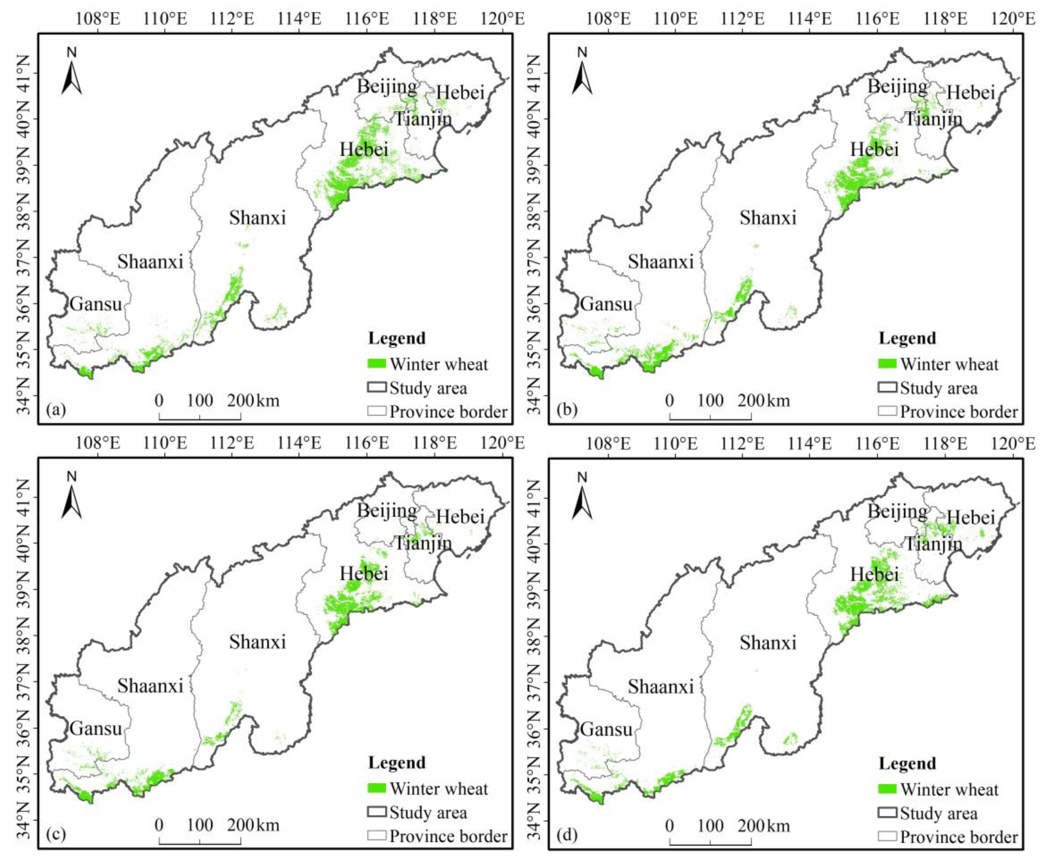
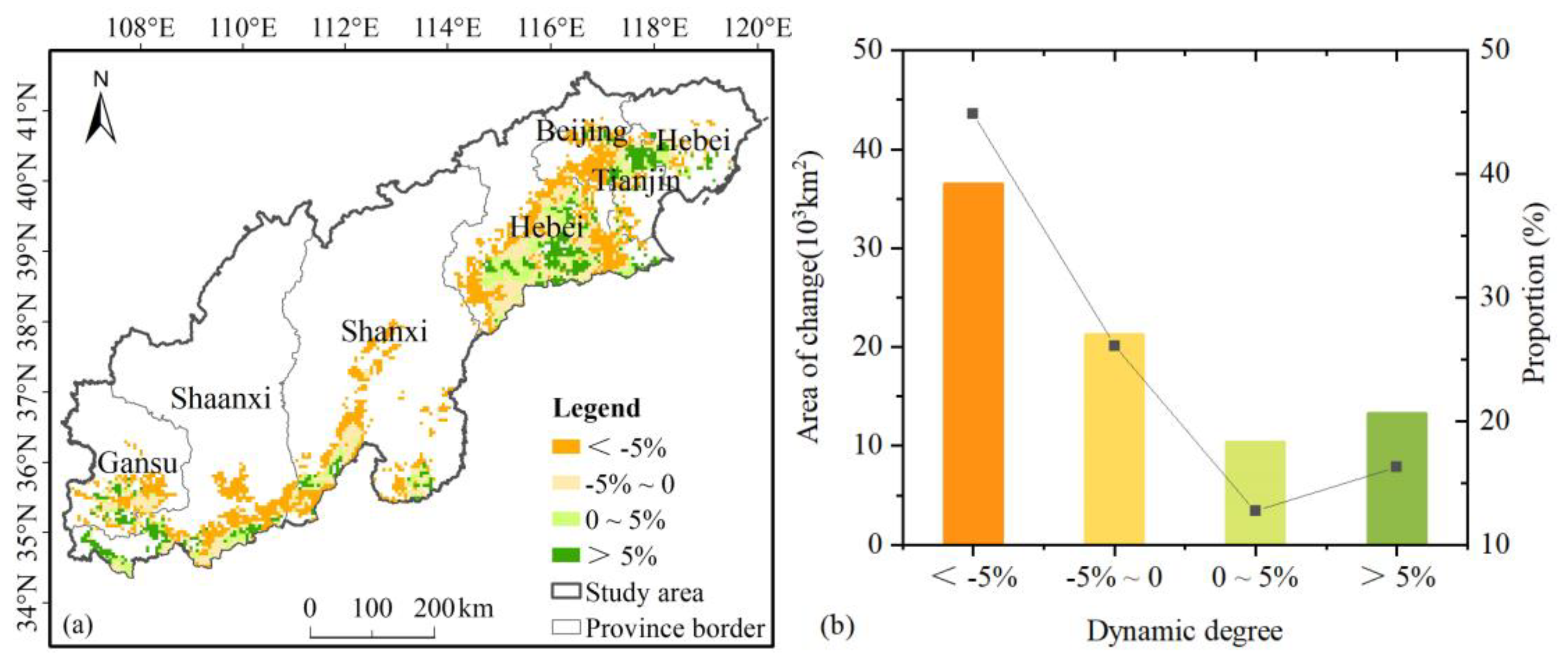
4.2. Spatiotemporal Dynamics of Winter Wheat Planting Area

The winter wheat planting area in northern China displayed a decreasing trend from 2001 to 2019. The planting area of winter wheat decreased significantly, from 16.0 × 10³ km² to 12.4 × 10³ km² during the period 2001–2014, and increased in 2019. In terms of spatial variation, the planting area in the transition zone of winter wheat planting decreased most obviously, particularly in the Shanxi and Shaanxi Provinces (Figure 6).

The Jenks optimization method was used to visually reflect the dynamic degree of spatial and temporal changes of the winter wheat planting area. Over the past 20 years, in general there has been a significant reduction in the dynamic degree of the change of winter wheat planting area (71% reduction) (Figure 7a). The trend was clearest in the northernmost planting transition zone of winter wheat (Figure 7b).

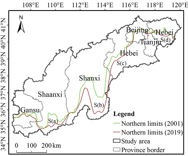
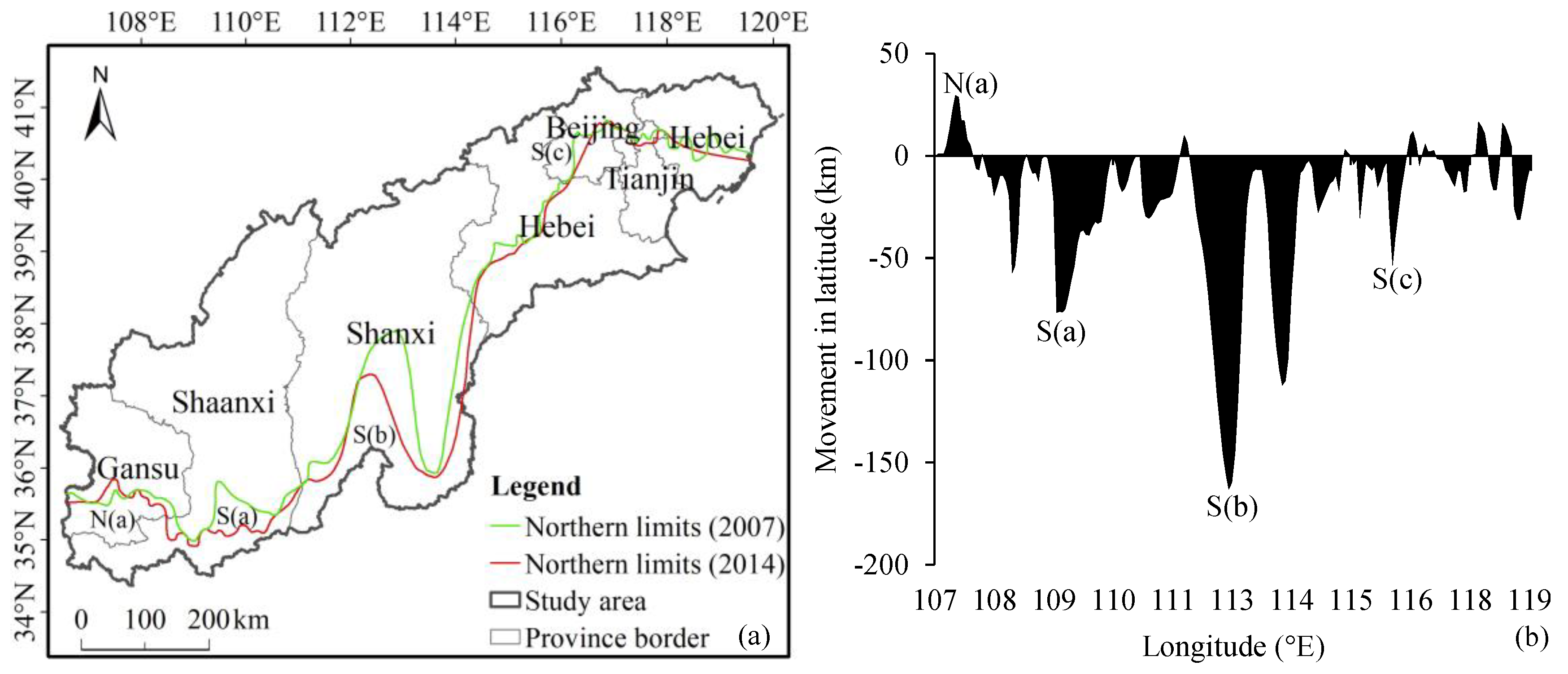
4.3. Latitudinal Dynamics of the NLWW during the Period 2001–2019

During the period 2001–2019, the NLWW showed a clear trend of southward movement, i.e., as an average for the entire study area, the NLWW moved 37 km southward. Specifically, it moved southward by 83 km in the area of transition between the Shaanxi Basin and Shaanxi Plateau (represented by S(a) in Figure 8a,b), by 189 km on the Shanxi Central Plain (represented by S(b) in Figure 8a,b), and by 46 and 56 km in the border area of the Hebei Plain and Hebei mountain ranges, respectively (represented by S(c) and S(d), respectively, in Figure 8a and Figure 8b).

In the past 20 years, the shift of the NLWW has exhibited a marked fluctuating trend of southward movement. During this migration, the amplitude of the shift reflected in each period has varied. The period with the most substantial southward movement was 2007–2014.

During the period 2001–2007, the average movement of the NLWW was 11 km southward. On the Loess Plateau of eastern Gansu, there was modest southward movement of 29 km (represented by S(a) in Figure 9a,b). The areas in which the NLWW moved southward more obviously were the Shanxi Central Plain (93 km; represented by S(b) in Figure 9a,b), and the border area of the Hebei Plain and Hebei mountain ranges (35 km; represented by S(c) in Figure 9a,b). However, northward movements of 44 and 30 km occurred at the Shaanxi–Gansu border and the Shaanxi–Shanxi border, respectively (represented by N(a) and N(b), respectively, in Figure 9a and Figure 9b).

During the period 2007–2014, the average movement of the NLWW was 23 km southward. It moved 76 km to the south in the transition area between the Shaanxi Basin and Shaanxi Plateau (represented by S(a) in Figure 10a,b). The area where the NLWW moved more obviously southward was the Shanxi Central Plain (163 km; represented by S(b) in Figure 10a,b). The NLWW shifted 53 km southward on the border area of the Hebei Plain and Hebei mountain (represented by S(c) in Figure 10a,b). In addition, there was northward movement of 29 km on the Loess Plateau of eastern Gansu (represented by N(a) in Figure 10a,b).

In comparison with the previous period, the NLWW generally showed only a slight trend of southward movement (4 km) during the period 2014–2019. The areas with southward movement were primarily the Shanxi Central Basin (47 km; represented by S(a) in Figure 11) and in the transition area between the Shaanxi Basin and Shaanxi Plateau (20 km). However, northward movement occurred at the northern end of the North China Plain (34 km; represented by N(a) in Figure 11).

4.4. Elevational Gradient Distributions of the NLWW during the Period 2001–2019

Over the past 20 years, a fluctuating trend of increase from east to west has been demonstrated in the elevation of the NLWW for each period (Figure 12a). In comparison with western areas, eastern parts exhibited clear changes in the elevation of the NLWW (i.e., winter wheat cultivation in high-elevation areas in the east gradually decreased), particularly in the border area of the Hebei Plain and Hebei mountain ranges. The elevation limit of winter wheat planting was approximately 1600 m. Overall, the amount of winter wheat planting in low-elevation areas gradually increased, and its planting centroid shifted slowly toward low-elevation areas (Figure 12b).

5. Discussion

We analyzed the latitudinal dynamics of the NLWW during the period 2001–2019 in northern China. This analysis indicated that the actual NLWW showed a clear trend of southward movement. In contrast, the potential NLWW showed considerable northward movement and westward expansion [10,43]. There was indeed a gap between the potential NLWW and the actual NLWW in China. Therefore, we analyzed the reasons for this gap.

5.1. Analysis of Driving Factors for the Gap Between the Potential NLWW and the Actual NLWW

Climate change has led to a northward shifting of the potential NLWW in China [44]. In general, the limit moves to the north during warm and wet periods, and it expands to the south during the cold and dry period [45]. Over the past five decades, the record of temperature in the growing season has demonstrated a significant increase in temperature [46]. Simultaneously, extremely arid areas on land have become increasingly humid, and increasingly favorable climatic conditions have made it possible to plant winter wheat at higher latitudes [47]. This has provided favorable climatic conditions for the northward migration of the potential NLWW [48]. The northward shift of the potential NLWW shows that the climatic resource conditions suitable for winter wheat planting are gradually expanding northward, but it does not mean that the actual winter wheat planting is moving to the north.

Through the interacting effects of human activities and climate change, the actual NLWW was formed under suitable climatic conditions, and moved southward. Human activities play a decisive role in the formation and change of the actual NLWW. Urbanization development, the migration of agricultural populations and comparative incomes, among other factors, affect the shift of the actual NLWW. In the areas where groups of cities are located, farmland resources have been repurposed to provide additional space for city development [49]. For example, the Development of Western China further accelerated urbanization after the year 2000 [50]. Rural labor has undergone a large-scale transfer to urban areas, resulting in the loss of famers engaged in winter wheat cultivation, which further led to a decline, or even non-planting, of winter wheat [51]. Large areas of farmland have been abandoned in some regions of northern China [52]. In comparison with other economic crops, winter wheat often succumbed to drought, freezing and insects [9], which elevated the risks and costs associated with winter wheat planting [53]. Hence, the large input–output gap associated with winter wheat planting often reduces the willingness of farmers to plant winter wheat [54]. Many farmers in transition areas of winter wheat cultivation prefer to plant less, or even no, winter wheat.

Government policy has also been a key driving force for actual NLWW changes. A series of ecological engineering projects has been applied in northern China [55]. The Grain for Green project encouraged farmland shrinkage by ecological restoration, especially in northern China [50]. This policy dictated that farmland that is unsuitable for cropping should be converted to woodland or grassland for ecological restoration. The winter wheat planting area significantly decreased during the period 2000–2010, mainly owning to the deployment of protection policies [41]. Agricultural incentive policies guided farmers to change cropping systems by subsidizing the reduction of winter wheat planting [54,56]. In addition, local governments have undertaken the supply-side structural reform of agriculture to adjust the planting structure [57]. For example, based on the natural resource conditions and production characteristics, Hebei Province’s central and southern regions have been regarded as the key development areas for strong gluten winter wheat. The winter wheat planting area in the region has increased in recent years. Further, winter wheat production was also affected by expanding irrigation infrastructure, the update of winter wheat varieties, purchase prices, and so forth [58].

5.2. Uncertainties in MODIS-Derived Winter Wheat Maps

Considering the impacts of unstable climate change, weather-related agricultural disasters and the quality of the MODIS and Landsat remote sensing data, the research period of 2001–2019 was divided into four years: 2001, 2007, 2014 and 2019. The MODIS-derived map of winter wheat for each of these years can represent the stable state of the winter wheat planting area. Compared with the curve shape-based algorithm and the winter bump method, the CBAH method incorporated the intraclass variability over large regions, and thus achieved higher accuracy for winter wheat mapping [18]. For the former two algorithms, clear commission errors occurred in winter wheat mapping (i.e., overestimations were confirmed in provincial census statistics and ground survey data). The characteristics for vegetation indices were relatively stable in smaller regions, but the two algorithms had difficulties in obtaining satisfactory results in larger regions [16]. Therefore, in our larger region of 380,000 km², we used the CBAH method to attain the most appropriate results for winter wheat mapping.

It is important to note that our actual NLWW was the NLWW of the core area of winter wheat planting extracted using the KDE method on the spatial scale of the MODIS data (i.e., 250 × 250 m). Some sections of the study area contain complex terrain, fragmented land and mixed crops, which would have an impact on the accuracy of the MODIS-derived mapping. For example, a small proportion of winter wheat planting was scattered and distributed within mountainous areas, where the natural growth environment is poor.

We applied the CBAH method to map winter wheat in the study area. There were uncertainties in the verification methods adopted. First, owing to the low spatial resolution of the MODIS EVI2 data, it was not possible to fully capture the scattered areas of winter wheat planting. Second, the extraction results of the winter wheat planting area were verified using agricultural census data; however, the agricultural census data have certain inherent errors. Moreover, an assessment of the degree of consistency in the spatial distribution could not be performed. For example, at the county level, in comparison with the agricultural census data, the MODIS-estimated area of winter wheat was underestimated or overestimated in certain counties [18]. Finally, Landsat validation was only performed for an area in the middle of the Hebei Plain where winter wheat planting is reasonably concentrated. In Shanxi, Shaanxi and eastern Gansu, no validation was possible due to a lack of data or data quality problems.

6. Conclusions

In the context of climate change, it is crucial to understand the spatiotemporal shifts of the NLWW in order to develop adaptation strategies and ensure food security in China. In this study, we extracted the actual NLWW for 2001, 2007, 2014 and 2019 in China, and quantitatively analyzed the directions and distances of the temporal and spatial changes. The CBAH method achieved good results for winter wheat mapping in this study area based on the MODIS-derived maps of the spatial distribution of winter wheat. In the past 20 years, there has been a significant decrease of winter wheat in the transition zone of winter wheat planting. It was found that the NLWW has exhibited a marked fluctuating trend of southward migration, and the average distance of movement was 37 km in latitude. Our results revealed that the elevation limit of winter wheat planting was approximately 1,600 m, and the centroid of the area of winter wheat planting has slowly shifted toward low-elevation areas. Human activities were the decisive factor for the formation and southward movement of the actual NLWW, while the northward movement of the potential NLWW was caused by climate warming and humidification, and there was a large gap between these two limits. Our study provides an important scientific reference for adaptation of the winter wheat cropping system to future climate change.

This study represents a pioneering investigation of NLWW extraction for a large area using MODIS time series data. The actual NLWW in northern China has exhibited a fluctuating trend of southward movement as a result of anthropogenic activities under suitable climatic conditions. Further research is needed to ascertain the mechanism whereby climatic factors and human activities might influence the formation and change of the actual NLWW.

References

1. Appels, R.; Eversole, K.; Stein, N.; Feuillet, C.; Keller, B.; Rogers, J.; Pozniak, C.J.; Choulet, F.; Distelfeld, A.; Poland, J.; et al. Shifting the limits in wheat research and breeding using a fully annotated reference genome. Science 2018, 361, eaar7191. [Google Scholar] [CrossRef] [Green Version]
2. Dong, J.; Lu, H.; Wang, Y.; Ye, T.; Yuan, W. Estimating winter wheat yield based on a light use efficiency model and wheat variety data. ISPRS J. Photogramm. Remote Sens. 2020, 160, 18–32. [Google Scholar] [CrossRef]
3. Zhao, C.; Liu, B.; Piao, S.; Wang, X.; Lobell, D.B.; Huang, Y.; Huang, M. Temperature increase reduces global yields of major crops in four independent estimates. Proc. Natl. Acad. Sci. USA 2017, 114, 9326–9331. [Google Scholar] [CrossRef] [Green Version]
4. Wang, H.; Vicente-serrano, S.M.; Tao, F.; Zhang, X.; Wang, P.; Zhang, C.; Chen, Y.; Zhu, D.; Kenawy, A.E. Monitoring winter wheat drought threat in Northern China using multiple climate-based drought indices and soil moisture during 2000–2013. Agric. For. Meteorol. 2016, 228–229, 1–12. [Google Scholar] [CrossRef]
5. Liu, Z.; Liu, Y.; Li, Y. Extended warm temperate zone and opportunities for cropping system change in the Loess Plateau of China. Int. J. Climatol. 2019, 39, 658–669. [Google Scholar] [CrossRef]
6. Wu, W.; Verburg, P.H.; Tang, H. Climate change and the food production system: Impacts and adaptation in China. Reg. Environ. Chang. 2014, 14, 1–5. [Google Scholar] [CrossRef] [Green Version]
7. Neset, T.S.; Wiréhn, L.; Opach, T.; Glaas, E.; Linnér, B.O. Evaluation of indicators for agricultural vulnerability to climate change: The case of Swedish agriculture. Ecol. Indic. 2019, 105, 571–580. [Google Scholar] [CrossRef]
8. Ray, D.K.; West, P.C.; Clark, M.; Gerber, J.S.; Prishchepov, A.V.; Chatterjee, S. Climate change has likely already affected global food production. PLoS ONE 2019, 14, 1–18. [Google Scholar] [CrossRef]
9. Olmstead, A.L.; Rhode, P.W. Adapting North American wheat production to climatic challenges, 1839–2009. Proc. Natl. Acad. Sci. USA 2011, 108, 480–485. [Google Scholar] [CrossRef] [Green Version]
10. Yang, X.; Chen, F.; Lin, X.; Liu, Z.; Zhang, H.; Zhao, J.; Li, K.; Ye, Q.; Li, Y.; Lv, S.; et al. Potential benefits of climate change for crop productivity in China. Agric. For. Meteorol. 2015, 208, 76–84. [Google Scholar] [CrossRef]
11. Zhang, Q.; Deng, Z.Y.; Zhao, Y.D.; Qiao, J. The impacts of global climatic change on the agriculture in northwest China. Acta Ecol. Sin. 2008, 28, 1210–1218. [Google Scholar] [CrossRef]
12. Wu, X.; Qi, Y.; Shen, Y.; Yang, W.; Zhang, Y.; Kondoh, A. Change of winter wheat planting area and its impacts on groundwater depletion in the North China Plain. J. Geogr. Sci. 2019, 29, 891–908. [Google Scholar] [CrossRef] [Green Version]
13. Gómez, C.; White, J.C.; Wulder, M.A. Optical remotely sensed time series data for land cover classification: A review. ISPRS J. Photogramm. Remote Sens. 2016, 116, 55–72. [Google Scholar] [CrossRef] [Green Version]
14. Song, Q.; Hu, Q.; Zhou, Q.; Hovis, C.; Xiang, M.; Tang, H.; Wu, W. In-season crop mapping with GF-1/WFV data by combining object-based image analysis and random forest. Remote Sens. 2017, 9, 1184. [Google Scholar] [CrossRef] [Green Version]
15. Tao, J.; Wu, W.; Zhou, Y.; Wang, Y.; Jiang, Y. Mapping winter wheat using phenological feature of peak before winter on the North China Plain based on time-series MODIS data. J. Integr. Agric. 2017, 16, 348–359. [Google Scholar] [CrossRef]
16. Sun, H.; Xu, A.; Lin, H.; Zhang, L.; Mei, Y. Winter wheat mapping using temporal signatures of MODIS vegetation index data. Int. J. Remote Sens. 2012, 33, 5026–5042. [Google Scholar] [CrossRef]
17. Yang, Y.; Tao, B.; Ren, W.; Zourarakis, D.P.; Masri, B.E.; Sun, Z.; Tian, Q. An improved approach considering intraclass variability for mapping winter wheat using multitemporal MODIS EVI images. Remote Sens. 2019, 11, 1191. [Google Scholar] [CrossRef] [Green Version]
18. Qiu, B.; Luo, Y.; Tang, Z.; Chen, C.; Lu, D.; Huang, H.; Chen, Y.; Chen, N.; Xu, W. Winter wheat mapping combining variations before and after estimated heading dates. ISPRS J. Photogramm. Remote Sens. 2017, 123, 35–46. [Google Scholar] [CrossRef]
19. Pan, Y.; Li, L.; Zhang, J.; Liang, S.; Zhu, X.; Sulla-Menashe, D. Winter wheat area estimation from MODIS-EVI time series data using the Crop Proportion Phenology Index. Remote Sens. Environ. 2012, 119, 232–242. [Google Scholar] [CrossRef]
20. Khan, A.; Hansen, M.C.; Potapov, P.V.; Adusei, B.; Pickens, A.; Krylov, A.; Stehman, S.V. Evaluating Landsat and RapidEye data for winter wheat mapping and area estimation in Punjab, Pakistan. Remote Sens. 2018, 10, 489. [Google Scholar] [CrossRef] [Green Version]
21. Skakun, S.; Vermote, E.; Roger, J.-C.; Franch, B. Combined Use of Landsat-8 and Sentinel-2A Images for Winter Crop Mapping and Winter Wheat Yield Assessment at Regional Scale. AIMS Geosci. 2017, 3, 163–186. [Google Scholar] [CrossRef] [PubMed]
22. Song, Y.; Wang, J. Mapping Winter Wheat Planting Area and Monitoring Its Phenology Using Sentinel-1 Backscatter Time Series. Remote Sens. 2019, 11, 449. [Google Scholar] [CrossRef] [Green Version]
23. Zhou, T.; Pan, J.; Zhang, P.; Wei, S.; Han, T. Mapping winter wheat with multi-temporal SAR and optical images in an urban agricultural region. Sensors 2017, 17, 1210. [Google Scholar] [CrossRef]
24. Skakun, S.; Franch, B.; Vermote, E.; Roger, J.C.; Becker-Reshef, I.; Justice, C.; Kussul, N. Early season large-area winter crop mapping using MODIS NDVI data, growing degree days information and a Gaussian mixture model. Remote Sens. Environ. 2017, 195, 244–258. [Google Scholar] [CrossRef]
25. Clauss, K.; Yan, H.; Kuenzer, C. Mapping paddy rice in China in 2002, 2005, 2010 and 2014 with MODIS time series. Remote Sens. 2016, 8, 434. [Google Scholar] [CrossRef] [Green Version]
26. Dempewolf, J.; Adusei, B.; Becker-Reshef, I.; Hansen, M.; Potapov, P.; Khan, A.; Barker, B. Wheat yield forecasting for Punjab Province from vegetation index time series and historic crop statistics. Remote Sens. 2014, 6, 9653–9675. [Google Scholar] [CrossRef] [Green Version]
27. Dong, J.; Xiao, X.; Zhang, G.; Menarguez, M.A.; Choi, C.Y.; Qin, Y.; Luo, P.; Zhang, Y.; Moore, B. Northward expansion of paddy rice in northeastern Asia during 2000-2014. Geophys. Res. Lett. 2016, 43, 3754–3761. [Google Scholar] [CrossRef] [Green Version]
28. Gao, F.; Anderson, M.C.; Zhang, X.; Yang, Z.; Alfieri, J.G.; Kustas, W.P.; Mueller, R.; Johnson, D.M.; Prueger, J.H. Toward mapping crop progress at field scales through fusion of Landsat and MODIS imagery. Remote Sens. Environ. 2017, 188, 9–25. [Google Scholar] [CrossRef] [Green Version]
29. Qiu, B.; Huang, Y.; Chen, C.; Tang, Z.; Zou, F. Mapping spatiotemporal dynamics of maize in China from 2005 to 2017 through designing leaf moisture based indicator from Normalized Multi-band Drought Index. Comput. Electron. Agric. 2018, 153, 82–93. [Google Scholar] [CrossRef]
30. Hu, Q.; Ma, Y.; Xu, B.; Song, Q.; Tang, H.; Wu, W. Estimating sub-pixel soybean fraction from time-series MODIS data using an optimized geographically weighted regression model. Remote Sens. 2018, 10, 491. [Google Scholar] [CrossRef] [Green Version]
31. Shi, W.; Liu, Y.; Shi, X. Contributions of climate change to the boundary shifts in the farming-pastoral ecotone in northern China since 1970. Agric. Syst. 2018, 161, 16–27. [Google Scholar] [CrossRef]
32. Yan, H.; Liu, F.; Qin, Y.; Niu, Z.; Doughty, R.; Xiao, X. Tracking the spatio-temporal change of cropping intensity in China during 2000-2015. Environ. Res. Lett. 2019, 14. [Google Scholar] [CrossRef]
33. Zhao, J.; Yang, Y.; Zhang, K.; Jeong, J.; Zeng, Z.; Zang, H. Does crop rotation yield more in China? A meta-analysis. F. Crop. Res. 2020, 245, 107659. [Google Scholar] [CrossRef]
34. Zhang, J.; Feng, L.; Yao, F. Improved maize cultivated area estimation over a large scale combining MODIS-EVI time series data and crop phenological information. ISPRS J. Photogramm. Remote Sens. 2014, 94, 102–113. [Google Scholar] [CrossRef]
35. Bégué, A.; Arvor, D.; Bellon, B.; Betbeder, J.; de Abelleyra, D.; Ferraz, R.P.D.; Lebourgeois, V.; Lelong, C.; Simões, M.; Verón, S.R. Remote sensing and cropping practices: A review. Remote Sens. 2018, 10, 99. [Google Scholar] [CrossRef] [Green Version]
36. Doktor, D.; Lausch, A.; Spengler, D.; Thurner, M. Extraction of plant physiological status from hyperspectral signatures using machine learning methods. Remote Sens. 2014, 6, 12247–12274. [Google Scholar] [CrossRef] [Green Version]
37. Hu, Q.; Wu, W.; Xia, T.; Yu, Q.; Yang, P.; Li, Z.; Song, Q. Exploring the use of google earth imagery and object-based methods in land use/cover mapping. Remote Sens. 2013, 5, 6026–6042. [Google Scholar] [CrossRef] [Green Version]
38. Zuo, L.; Zhang, Z.; Zhao, X.; Wang, X.; Wu, W.; Yi, L.; Liu, F. Multitemporal analysis of cropland transition in a climate-sensitive area: A case study of the arid and semiarid region of northwest China. Reg. Environ. Chang. 2014, 14, 75–89. [Google Scholar] [CrossRef]
39. Bonnier, A.; Finné, M.; Weiberg, E. Examining Land-Use through GIS-Based Kernel Density Estimation: A Re-Evaluation of Legacy Data from the Berbati-Limnes Survey. J. F. Archaeol. 2019, 44, 70–83. [Google Scholar] [CrossRef] [Green Version]
40. Pilø, L.; Finstad, E.; Ramsey, C.B.; Martinsen, J.R.P.; Nesje, A.; Solli, B.; Wangen, V.; Callanan, M.; Barrett, J.H. The chronology of reindeer hunting on Norway’s highest ice patches. R. Soc. Open Sci. 2018, 5. [Google Scholar] [CrossRef] [Green Version]
41. Li, S.; Sun, Z.; Tan, M.; Guo, L.; Zhang, X. Changing patterns in farming–pastoral ecotones in China between 1990 and 2010. Ecol. Indic. 2018, 89, 110–117. [Google Scholar] [CrossRef]
42. Yang, P.; Shibasaki, R.; Wu, W.; Zhou, Q.; Chen, Z.; Zha, Y.; Shi, Y.; Tang, H. Evaluation of MODIS land cover and LAI products in cropland of north china plain using in situ measurements and landsat TM Images. IEEE Trans. Geosci. Remote Sens. 2007, 45, 3087–3097. [Google Scholar] [CrossRef]
43. Yang, X.; Liu, Z.; Chen, F. The Possible Effect of Climate Warming on Northern Limits of Cropping System and Crop Yield in China. Agric. Sci. China 2011, 10, 585–594. [Google Scholar] [CrossRef]
44. Li, T.; Long, H.; Zhang, Y.; Tu, S.; Ge, D.; Li, Y.; Hu, B. Analysis of the spatial mismatch of grain production and farmland resources in China based on the potential crop rotation system. Land Use Policy 2017, 60, 26–36. [Google Scholar] [CrossRef]
45. Shi, X.; Shi, W. Review on boundary shift of farming-pastoral ecotone in northern China and its driving forces. Trans. Chin. Soc. Agric. Eng. 2018, 34, 1–11. [Google Scholar] [CrossRef]
46. Liu, Z.; Liu, Y.; Li, Y. Anthropogenic contributions dominate trends of vegetation cover change over the farming-pastoral ecotone of northern China. Ecol. Indic. 2018, 95, 370–378. [Google Scholar] [CrossRef]
47. Donat, M.G.; Lowry, A.L.; Alexander, L.V.; O’Gorman, P.A.; Maher, N. More extreme precipitation in the world’s dry and wet regions. Nat. Clim. Chang. 2016, 6, 508–513. [Google Scholar] [CrossRef]
48. Shi, W.; Tao, F.; Liu, J.; Xu, X.; Kuang, W.; Dong, J.; Shi, X. Has climate change driven spatio-temporal changes of cropland in northern China since the 1970s? Clim. Chang. 2014, 124, 163–177. [Google Scholar] [CrossRef]
49. Jiang, L.; Deng, X.; Seto, K.C. The impact of urban expansion on agricultural land use intensity in China. Land Use Policy 2013, 35, 33–39. [Google Scholar] [CrossRef]
50. Liu, J.; Zhang, Z.; Xu, X.; Kuang, W.; Zhou, W.; Zhang, S.; Li, R.; Yan, C.; Yu, D.; Wu, S.; et al. Spatial patterns and driving forces of land use change in China during the early 21st century. J. Geogr. Sci. 2010, 20, 483–494. [Google Scholar] [CrossRef]
51. Chen, R.; Ye, C.; Cai, Y.; Xing, X.; Chen, Q. The impact of rural out-migration on land use transition in China: Past, present and trend. Land Use Policy 2014, 40, 101–110. [Google Scholar] [CrossRef]
52. Xiao, G.; Zhu, X.; Hou, C.; Xia, X. Extraction and analysis of abandoned farmland: A case study of Qingyun and Wudi counties in Shandong Province. J. Geogr. Sci. 2019, 29, 581–597. [Google Scholar] [CrossRef] [Green Version]
53. Lesk, C.; Rowhani, P.; Ramankutty, N. Influence of extreme weather disasters on global crop production. Nature 2016, 529, 84–87. [Google Scholar] [CrossRef] [PubMed]
54. Xie, H.; Cheng, L.; Lv, T. Factors influencing farmer willingness to fallow winter wheat and ecological compensation standards in a groundwater funnel area in Hengshui, Hebei Province, China. Sustainability 2017, 9, 839. [Google Scholar] [CrossRef] [Green Version]
55. Wang, S.; Fu, B.; Piao, S.; Lü, Y.; Ciais, P.; Feng, X.; Wang, Y. Reduced sediment transport in the Yellow River due to anthropogenic changes. Nat. Geosci. 2016, 9, 38–41. [Google Scholar] [CrossRef]
56. Liu, Z.; Yang, P.; Wu, W.; You, L. Spatiotemporal changes of cropping structure in China during 1980–2011. J. Geogr. Sci. 2018, 28, 1659–1671. [Google Scholar] [CrossRef] [Green Version]
57. Zhou, Y.; Shi, W.; Wang, Q.; Zhang, F. The Countermeasure Research on the Agricultural Supply-side Structural Reform in Liaoning Province. Adv. Econ. Bus. Manag. Res. 2018, 71, 186–189. [Google Scholar] [CrossRef]
58. Tanaka, A.; Takahashi, K.; Masutomi, Y.; Hanasaki, N.; Hijioka, Y.; Shiogama, H.; Yamanaka, Y. Adaptation pathways of global wheat production: Importance of strategic adaptation to climate change. Sci. Rep. 2015, 5, 2–11. [Google Scholar] [CrossRef]
Figure 1. Geographic location of the study area. The borders of the MODIS and Landsat scenes are shown on the map. The spatial distribution of ground survey sites and the locations of agrometeorological sites are also indicated. Elevation information was derived from a digital elevation model with 90-m spatial resolution.
Remotesensing 12 02382 g001
Figure 2. Basic details of the sampling point data. The figure includes the source of the sampling point data and the application of the data in 2001, 2007, 2014 and 2019.
Remotesensing 12 02382 g002
Figure 3. Schematic of phenological index extraction of winter wheat. Black solid line represents winter wheat, black dotted line represents unknown pixels, red arrow represents the EVE, blue arrow represents the EVL, SDS (light green shaded rectangular belt) represents the seedling stage, HDS (green shaded rectangular belt) represents the heading stage, and HTS (yellow shaded rectangular belt) represents the harvesting stage.
Remotesensing 12 02382 g003
Figure 4. Maps of winter wheat in the 123033 tile area derived from (a) Landsat and (b) MODIS data in 2001, 2007, 2014 and 2019.
Remotesensing 12 02382 g004
Figure 5. Correlation analysis between winter wheat statistics and MODIS-estimated area in (a) 2001, (b) 2007 and (c) 2014 at the county level.
Remotesensing 12 02382 g005
Figure 6. Spatial distribution of winter wheat planting area based on MODIS in 2001 (a), 2007 (b), 2014 (c) and 2019 (d).
Remotesensing 12 02382 g006
Figure 7. Dynamic degree analysis of spatial and temporal changes of winter wheat planting area from 2001 to 2019. (a) The dynamic degree of the winter wheat planting area changes in a 5 × 5-km grid; (b) The change area and proportion of winter wheat dynamic degree in a 5 × 5-km grid. (Dark orange is <−5% dynamic degree, orange is −5~0% dynamic degree, light green is 0~5% dynamic degree, green is >5% dynamic degree.).
Remotesensing 12 02382 g007
Figure 8. (a) Derived extent of the northern limit of winter wheat (NLWW) and (b) latitudinal movement of the NLWW during the period 2001–2019. (Red solid line represents the NLWW in 2019, green solid line represents the NLWW in 2001, black bars indicate latitudinal movement of the NLWW, and S(a, b, c, d) represent typical points of southward migration.).
Remotesensing 12 02382 g008
Figure 9. (a) Derived extent of the NLWW and (b) latitudinal movement of the NLWW during the period 2001–2007 (Red solid lines show NLWW at end of period, green solid lines show NLWW at beginning of period, black bars indicate latitudinal movement of NLWW, S(a, b, c) represent typical points of southward migration, and N(a, b) represent typical points of northward migration.).
Remotesensing 12 02382 g009
Figure 10. (a) Derived extent of the NLWW and (b) latitudinal movement of the NLWW during the period 2007–2014 (Red solid lines show NLWW at end of period, green solid lines show NLWW at beginning of period, black bars indicate latitudinal movement of NLWW, S(a, b, c) represent typical points of southward migration, and N(a) represents typical points of northward migration.).
Remotesensing 12 02382 g010
Figure 11. (a) Derived extent of the NLWW and (b) latitudinal movement of the NLWW during the period 2014–2019. (Red solid lines show NLWW at end of period, green solid lines show NLWW at beginning of period, black bars indicate latitudinal movement of NLWW, S(a) represent typical points of southward migration, and N(a) represent typical points of northward migration.).
Remotesensing 12 02382 g011
Figure 12. Change of elevation of the NLWW during the period 2001–2019. (Green, blue, orange and dark orange solid lines in (a) are the elevation change curves, and in (b) represent the cumulative distribution function curves of the statistical quantity of different normalized elevation values in 2001, 2007, 2014 and 2019, respectively.).
Remotesensing 12 02382 g012