Abstract
Assessing plant population of cotton is important to make replanting decisions in low plant density areas, prone to yielding penalties. Since the measurement of plant population in the field is labor intensive and subject to error, in this study, a new approach of image-based plant counting is proposed, using unmanned aircraft systems (UAS; DJI Mavic 2 Pro, Shenzhen, China) data. The previously developed image-based techniques required a priori information of geometry or statistical characteristics of plant canopy features, while also limiting the versatility of the methods in variable field conditions. In this regard, a deep learning-based plant counting algorithm was proposed to reduce the number of input variables, and to remove requirements for acquiring geometric or statistical information. The object detection model named You Only Look Once version 3 (YOLOv3) and photogrammetry were utilized to separate, locate, and count cotton plants in the seedling stage. The proposed algorithm was tested with four different UAS datasets, containing variability in plant size, overall illumination, and background brightness. Root mean square error (RMSE) and R2 values of the optimal plant count results ranged from 0.50 to 0.60 plants per linear meter of row (number of plants within 1 m distance along the planting row direction) and 0.96 to 0.97, respectively. The object detection algorithm, trained with variable plant size, ground wetness, and lighting conditions generally resulted in a lower detection error, unless an observable difference of developmental stages of cotton existed. The proposed plant counting algorithm performed well with 0–14 plants per linear meter of row, when cotton plants are generally separable in the seedling stage. This study is expected to provide an automated methodology for in situ evaluation of plant emergence using UAS data.
1. Introduction
In cotton (Gossypium hirsutum L.) production, early crop establishment is a critical stage that determines the yield potential of a given field. Yield potential is initially limited by the density of cotton plants and may be further impacted by unfavorable weather conditions, as well as disease and insect pressure [1,2,3,4]. Cotton yield can be maximized when plant density is 7–10 plants per linear meter of row and rapidly decreases below 5 plants per linear meter of row, for less indeterminate varieties planted in the Texas High Plains [5]. Therefore, a replanting decision should be made during the limited planting season when plant density is below an acceptable level [6].
One of the most common ways to evaluate plant density is manually counting the number of plants in 1/1000th of an acre (4047 m2) in the field [7]. The method consists of counting cotton seedlings along a specified distance that is equivalent to 1/1000th of an acre with respect to row spacing and multiplying the count by 1000 to estimate the number of plants per acre. The procedure should be repeated approximately 10 times in different locations and patterns to reduce sampling bias. Although this method is simple and straightforward, sampling bias can exist when the collected samples are not representative with respect to sampling location, and within-field variability is too high. Additionally, manual plant population assessment is time-consuming and labor-intensive.
Previous research has proved that unmanned aircraft systems (UAS; DJI Mavic 2 Pro, Shenzhen, China) can provide an accurate and consistent measurement of plant phenotypic traits at field scales [8,9,10]. This is achieved by leveraging high spatial and temporal resolution remote sensing data collected by UAS integrated with advanced sensors [11]. In this regard, the implementation of UAS in agricultural applications can help alleviate the issue of sampling bias, and possibly substitute manual field measurements in some instances. Most of the UAS-based research of cotton has been primarily conducted to acquire plant phenotypic data to evaluate plant vigor or stress level [12]. Plant physiological traits, such as canopy cover and height, are one of the most fundamental outcomes derived from UAS data as they generally control energy capture and water use efficiency [9,13]. Vegetation indices calculated from the combination of multispectral data can be utilized to characterize high yielding cotton varieties for plant breeding purposes [14], or to investigate effects of different management practices [15,16]. The spectral response of cotton root rot or spider mite infestation in a plant canopy can be used to identify damaged areas and monitor the progress of the disease [17,18]. In addition, UAS-derived plant phenotypic data can be exploited to quantify open cotton bolls in the field or to estimate yield [19,20].
For remote sensing based plant counting of cotton, a plant counting procedure based on maximum likelihood classification was suggested to detect cotton pixels in orthomosaic images, followed by a complimentary process of estimating plant count, when multiple cotton plants are overlapping [21]. To apply this approach, however, statistical relationships between the total number of plants and the average area of clustered plants should be re-calculated considering days after planting (DAP), cotton varieties, or region. A machine learning-based plant counting method was also proposed using hyperspectral UAS data [22]. Cotton pixels were extracted by normalized difference vegetation index (NDVI) thresholding, then multiple decision trees were used to estimate plant counts in regions where plants are clustered. Geometric attributes of the plant canopy were then fed into the machine learning model to retrieve plant counts. However, the above approach does not provide geolocation of individual plants. In addition, these techniques require a priori information of geometry or statistical properties of plant canopy features, and the input information can change depending on the developmental stage of cotton plants, field conditions, or lighting conditions. Consequently, the statistical or machine learning model of the previous approach should be adjusted for specific datasets.
Several pieces of research were conducted to determine image-based plant count of monocotyledons, including wheat and maize, in a highly dense environment [23,24,25]. Each of these studies relied on different plant counting algorithms to count plants, but the processing parameters or threshold values used in these algorithms require fine-tuning, depending on plant developmental stages or image statistics, as mentioned in above cases for plant counting of cotton.
UAS or satellite remote sensing data have also been used to count trees. In recent studies, image processing algorithms were applied to detect and geolocate individual trees in oil palm or olive farms, where trees are planted in a regularly spaced pattern [26,27]. A larger uncertainty is expected when delineating individual tree crowns (ITC) in a natural forest environment, and many object-based image analysis or region growing techniques have been developed to address this issue [28]. Remote sensing data, combined with object-based image analysis methods, also indicates the possibility of such algorithms in counting row crops [26,29]. In comparison with the research on counting trees, counting and geolocating of cotton in cropping systems requires the separation of plants, where the ratio of plant density to plant size is much higher in the planting row direction.
In this study, we propose a plant counting algorithm that can be applied to UAS data with variable plant size and field conditions, using You Only Look Once version 3 (YOLOv3), a deep learning-based object detection framework, and UAS photogrammetry. This approach can separate and geolocate individual cotton plants during the seedling stage, and the overall procedure requires a minimal number of input parameters for automation. In the object detection stage, YOLOv3 is applied on raw UAS images to fully take advantage of their higher spatial resolution, rather than applying the method on an orthomosaic image. This study aims to contribute to the growing area of in situ evaluation of plant emergence, as well as possible precision field management applications, by detecting objects of interest from UAS images.
2. Materials and Methods
2.1. Study Area and Plant Count Collection
The study area was located at the Texas A&M AgriLife Research and Extension Center at Corpus Christi, Texas, United States. The Köppen climate classification for this area is humid subtropical, characterized by high temperatures and evenly distributed precipitation throughout the year [30]. Three cotton cultivars were planted, targeting four different plant densities (3, 6, 9, and 12 plants per linear meter of row) on 5 April 2019. Each treatment was replicated four times. Plots were 56 rows wide by 11 m long and the cotton was planted in a North–South row orientation with a 1-m wide alley. Emergence of cotton seedlings started about 7 DAP, however, seedling survival rate varied between treatments affecting the final plant population. To consider the spatial variability of plant germination, the number of plants in 1 m by 1 m grids was quantified by a visual assessment of a UAS-derived orthomosaic image of 15 April. The grid-level plant count was used as a reference measurement to be compared with results from the proposed methodology (Figure 1).
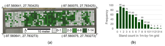
Figure 1.
Plant count of the entire study area at the grid level (1 m2) (a) and its histogram (b). Plant count assessed by visual inspection of Unmanned Aircraft Systems (UAS)-derived orthomosaic image.
2.2. UAS Data Collection
Input UAS data were collected using a DJI Mavic 2 Pro quadcopter equipped with a red, green, blue (RGB) Hasselblad L1D-20c camera. The onboard camera captured images with a 20-megapixel (5472 × 3648 pixels) CMOS sensor. Flight missions were conducted at 10 m above ground level (AGL) with 75% front and side overlap, resulting in a ground sampling distance (GSD) of 2.5 mm per pixel. Approximately 240 images were taken during each mission. Multiple UAS data were acquired between DAP 10–20 to verify that the proposed approach performed, even when within-row plant canopy was overlapping. (Table 1). Temporal variation in overall illumination (e.g., sun angle and cloud cover), soil wetness, and plant size allowed us to test the performance of the plant counting algorithm in diverse field conditions (Figure 2). In this study, a precise measurement of camera location or ground control points (GCP) were not available because the Mavic 2 Pro platform lacks a real time kinematics (RTK) GPS capability and a GCP survey was not performed. The location error of the UAS used in this study is less than 5 m, therefore, adjustment of camera locations by structure from motion (SfM) procedure was mandatory, to precisely project plant locations in image coordinates to the ground surface.

Table 1.
Summary of Unmanned Aircraft Systems (UAS) data collection.
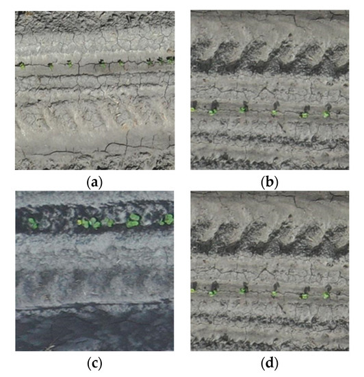
Figure 2.
Temporal variation in overall illumination, soil wetness, and plant size from zoomed-in images (416 × 416 pixels) of raw Unmanned Aircraft Systems (UAS) data collected on (a) 15 April, (b) 16 April, (c) 18 April, and (d) 24 April. Each image was taken from different locations.
2.3. Geospatial Object Detection Framework for Plant Counting
The proposed UAS-based plant counting framework consists of three core steps: (1) UAS data pre-processing, using a structure from Motion (SfM), (2) YOLOv3-based plant detection, and (3) image coordinates to ground surface projection using sensor orientation parameters. Each step is built upon a distinct sub-procedure designed to generate output used for the following steps (Figure 3).
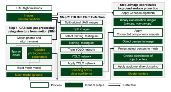
Figure 3.
Plant counting procedure using Unmanned Aircraft Systems (UAS) and the You Only Look Once version 3 (YOLOv3) object detection algorithm.
2.3.1. UAS Data Pre-Processing Using Structure from Motion (SfM)
Structure from motion (SfM) is an image-based three-dimensional (3D) reconstruction method that enables generation of high-resolution 3D data using consumer-grade cameras [31,32]. Multiple overlapping images are used by the SfM to estimate the metric characteristics of the camera (internal orientation, IO) for photogrammetric processes, and the exact position and orientation of the camera (external orientation, EO) when the photograph was taken. Local features such as corners or edges in the images are extracted by scale-invariant feature transform (SIFT), or one of its variant algorithms, subsequently, the feature points are matched across image pairs to optimize IO and EO [33]. During this procedure, valid key points that exist in image pairs are extracted as a sparse point cloud. A dense point cloud is generated by pairwise depth map computation [34] or multi view stereo (MVS) techniques, using information from the sparse cloud [35,36]. A surface model is created as a mesh or digital surface model (DSM) structure by applying a simplification algorithm to the sparse or dense point cloud. The surface models are then used to rectify geometric distortions in the original perspective images to generate an orthomosaic image.
In this study AgiSoft Metashape (Agisoft LLC, St. Petersburg, Russia) was used for SfM processing to build a ground mesh model. The original UAS images were used as input to the SfM pipeline. After the photo alignment step, initial camera positions were calculated to generate a sparse point cloud. A mesh surface was derived from the sparse point cloud because the proposed methodology only requires a low-detail surface rather than a high-fidelity model. The photogrammetric parameters (IO and EO), optimized during the SfM process, were used in the image coordinates to ground surface projection step.
2.3.2. YOLOv3-Based Plant Detection
The second step of the plant counting algorithm was identifying cotton plants from the raw UAS image set. The YOLOv3 model was used to obtain the location and size of individual plants in individual images [37]. YOLOv3 performs localization and object classification simultaneously by analyzing image data through its neural network, where the information flows without internal iterations. In general, YOLOv3 is faster than many deep learning models, including Single Shot Detector (SSD), Faster R-CNN, and RetinaNet [38]. The network structure and outcomes of YOLOv3, including bounding box coordinates, box confidence score, and conditional class probabilities are shown in Figure 4. The box confidence score refers to the likelihood of object presence in the corresponding bounding box, and the conditional class probability refers to the probability that the object belongs to a specific class. In its reference stage, class confidence score is used as a combined measure for both classification and localization. The class confidence score is calculated as a product of box confidence score and conditional class probability.
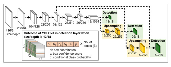
Figure 4.
Network architecture of YOLOv3 and its outcome.
In YOLOv3, there are three prediction blocks that are connected to the previous layer, with different levels of detail [37]. This allows YOLOv3 to detect small objects with about 50% and 25% of their original size. The upsampling feature can be particularly effective when plant size varies in UAS images due to the differences in plant developmental stage or distance between the camera and an object.
The rationale of our UAS-based plant counting was to minimize information loss by using the original UAS images instead of an orthomosaic image in the object detection process. Although an alternative approach that uses the orthomosaic image with image processing algorithms could be designed, it could be disadvantageous, because of potential problems related to image distortion in the orthomosaic image, which can occur since the SfM reconstructs objects from multiple images of a target [31]. When wind causes movements of a target plant in multiple images, the local feature points are not well aligned across the image pairs and the SfM process can lead to the absence of valid feature points or blurring of the target. Furthermore, GSD of an orthomosaic image is generally coarser than that of raw images. Due to these problems, utilizing the raw UAS images in which the target object is well defined (i.e., clear edge and texture) can be beneficial when detecting individual plants.
One of the challenges when detecting target objects from UAS imagery is lower detection accuracy, caused by the small target object in the input image. Many deep learning models, including YOLOv3, use multi-scale networks or region proposals to overcome this problem. A small object detection task in computer vision is generally aimed at detecting objects approximately less than, or equal to, 32 × 32 pixels in an image space of 640 × 640 pixels, whereas the object size in this study ranged from 10 × 10 to 40 × 40 pixels in the image space of 5472 × 3648 pixels [39,40]. To increase the relative size of objects in the images, all raw UAS images were split into non-overlapping image blocks, sized 416 by 416 pixels (Figure 5).
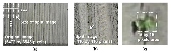
Figure 5.
Example of (a) raw UAS image collected on 15 April 2019 and (b) split image used for object detection, where (c) cotton seedling appears approximately in 15 by 15 pixels.
In order to train the YOLOv3 models, training and testing images were chosen from the split image dataset. The total number of split images for each UAS dataset in Table 1 was approximately 25,000 (240 raw images for each UAS dataset, 104 split images for each raw image: 240 × 104 = 24,960), and 300 split images were randomly selected for labeling. Cotton plants in the 300 images were manually labeled with center coordinates and the size of bounding box. The labeled images were then divided into 200, and 100, images as a training and testing set, respectively (Models 1–4 in Table 2). Six additional datasets were generated by combining the training and testing data of Models 1–4 in order to test the robustness of the plant counting algorithm when a larger number of input data, with an increased variability in target object (i.e., plant shape and size), are used. For this work, cotton plants with different sizes and shapes (Table 1, Figure 5) were labeled as a common cotton class. While creating additional classes for different developmental stages may be beneficial in in-season crop management applications, a single-class model was used in this study, since it could provide simplicity and efficiency for the plant counting algorithm. YOLOv3 models with the largest mean average precision (mAP) and F1 score were saved and used in the image coordinates to ground surface projection. General hyperparameters used for training the YOLOv3 network were as follows: momentum = 0.9, to help YOLOv3 network avoid local minima and converge faster; learning rate = 0.001, to control the speed of convergence with respect to the loss gradient; maximum iteration = 2000, to optimize error and avoid overfitting; decay = 0.0005, to prevent weights growing too large; saturation, exposure, hue = 1.5, 1.5, 0.1, to randomly change colors of images and reduce overfitting.
Table 2.
YOLOv3 cotton detection models generated from different training and testing data.
The performance of the YOLOv3 object detection was evaluated using the F1 score and mAP. The F1 score is the harmonic mean of precision and recall, and one of the most widely used accuracy measures utilized in image classification. The precision is defined by the number of true positive responses over the number of true positives plus the number of false positives, and the recall is defined by the number of the true positive responses over the number of true positives plus the number of false negatives. To calculate F1 scores, prediction results with a class confidence score over 0.25 were used [37,38]. In addition, mAP was also evaluated, which is an accuracy term commonly used in deep learning applications [41,42]. In essence, mAP is the area under the precision-recall curve where all prediction results were ranked in descending order of the class confidence score. To obtain mAP, objects with intersection over union (IoU) over 50% were used [37,38]. IoU measures how close the ground truth bounding box and predicted bounding box are, and it is calculated by the area of intersect divided by area of union.
2.3.3. Fine-Tuning of Object Center
Initially, it was expected that bounding boxes detected by the YOLOv3 algorithm would include a cotton plant at the geometric center of the boxes. An experimental analysis with 100 random object detection results revealed that there are small but considerable differences between bounding box centers and object centers (Figure 6).
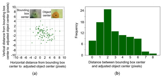
Figure 6.
Displacement between bounding box center and object center in a (a) horizontal and vertical direction, with (b) the histogram of the distance. The adjusted object center location was calculated as the geometric center of canopy pixels derived by a Canopeo-based algorithm [43].
To address this issue, the location of an accurate object center was determined by applying the Canopeo algorithm to generate a binary canopy map, and by performing connected components analysis to calculate centroid of the canopy within the bounding box region [43,44]. A pixel-level classification using the Canopeo algorithm was adopted to classify canopy and non-canopy pixels (green vs. non-green) from raw RGB images [43]. The canopy classification images generated by this step were then clipped using the bounding box coordinates retrieved from YOLOv3. Afterwards, connected components analysis was applied to the clipped images to delineate the canopy region within the bounding box in each canopy classification image [45,46]. The geometric center of the canopy region in the bounding box was calculated and exported as image coordinates of the original raw UAS image. The fine-tuning process for plant center was appended to the YOLOv3 object detection, before projecting center coordinates to the ground surface model (Figure 7).
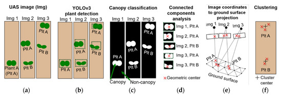
Figure 7.
Schematic diagram of overall plant detection procedure: (a) UAS data acquisition, (b) object detection using YOLOv3, (c) binary classification of canopy and non-canopy pixels, (d) plant center adjustment by connected components analysis, (e) localization of object detection results by UAS photogrammetry, and (f) extraction of average plant centers using agglomerative clustering algorithm.
If no canopy pixel was found within a bounding box, no coordinates were exported for the prediction. This may happen when the prediction of YOLOv3 is a false positive or when the Canopeo algorithm fails to detect canopy pixels. The latter case occurs mostly when yellow cotyledons or dried leaves are present. Although detecting dried plants is not in the scope of this study, an object detection approach similar to the proposed method could be implemented to locate dried plants by using the bounding box information and a fine-tuning algorithm for yellowish plant pixels.
Estimation of plant center by a Canopeo-based method was considered reliable because the Canopeo algorithm generally performs well with classifying canopy and non-canopy pixels, and the geometric center of the canopy pixels is found within the canopy area in most cases. Bounding box information retrieved from YOLOv3 is still necessary in this process, to define the approximate area in which each plant is located, especially for overlapping plants.
The experimental results indicated that 97% of the bounding box centers were located within 6 pixels from the object centers, determined by the Canopeo algorithm, and the other 3% were found to be up to 8 pixels away from the object centers (Figure 6b). Eight pixels in the raw image was equivalent to 20 mm on the ground surface, which may be acceptable and easy to compensate for when plant spacing is significantly wider than 40 mm. However, plant spacing may be less than 40 mm in some instances due to factors, such as planting method, field equipment, germination, seed quality, or field conditions, among others [47,48,49,50]. Accordingly, the projected plant centers of the clustered canopy might scatter in a continuous pattern along the major axis of the overlapping plants when the bounding box center is used for ground surface projection. The proposed algorithm in this study uses the geometric center of the canopy object derived by a Canopeo-based method to minimize the uncertainty of the object center location.
2.3.4. Image Coordinates to Ground Surface Projection
The geographic coordinates of each object center were calculated by projecting adjusted object centers onto the ground surface using AgiSoft Metashape (Agisoft LLC, St. Petersburg, Russia). In the beginning steps, the object center in the image coordinate system was calibrated by IO and transformed to a vector in a camera coordinate system. The vector in the camera coordinate system was transformed to another vector in Euclidean space by using EO parameters. Subsequently, a ray, starting from the perspective of the center of camera to the object center, was defined to calculate the intersection point between the ray and the ground surface model (Figure 3 and Figure 7). In addition to the geographic coordinates calculation, two additional metrics were considered in the process, i.e., radial distance from fiducial center to object center, and the class confidence score, calculated from the YOLOv3 algorithm. The additional metrics were used to reduce the number of detected objects, while removing the objects that might have larger location errors, induced by object detection and projection process.
Since the UAS images were acquired with significant overlaps, a single plant will be detected from multiple raw images, and it can be represented as multiple object centers when projected on the ground surface mesh. Therefore, an agglomerative hierarchical clustering algorithm was applied to merge the plant centers of a plant into a cluster, and to retrieve the center point of each cluster [51,52]. The agglomerative clustering algorithm first assigns each plant center as an individual cluster, and then successively merges clusters until a distance measure, between adjacent clusters, becomes bigger than a threshold value. In this study, Ward’s minimum variance method was used to measure distance between two clusters (Equation (1)) [51]:
where Ci and Cj mean two clusters; Cij means union of the two clusters; ri, rj, and rij mean the centroid of the corresponding cluster. The clustering technique was applied to the projected centers of detected plants, and the resultant cluster centers were counted in each 1 m by 1 m grid. The number of cluster centers was compared with the reference plant count previously obtained.
DWard = ∑x∈Ci (x − ri)2 + ∑x∈Cj (x − rj)2 + ∑x∈Cij (x − rij)2
3. Results and Discussion
3.1. Quality of Iput Data
An experiment was performed to confirm the consistency of object detection accuracy with the labeled data used in the study. From 300 labeled images of each flight (union of the training and testing set of Models 1–4 in Table 2), training and testing images were randomly chosen in a 2-to-1 split, and mAP was investigated as a measure of detection accuracy. This experiment was repeated 30 times for each labeled image of Models 1–4, to obtain average and standard deviation of mAP. The average mAP values of 85.1, 87.0, 78.3, and 72.3%, and standard deviations of 1.9, 2.7, 3.9, and 5.7 were observed from the datasets of 15, 16, 18, and 24 April (input dataset of Models 1–4), respectively (Figure 8). From models using the 15 April to 18 April datasets (Models 1–3), average values of mAP over 78% were observed, with standard deviations less than 4%, and the performance of object detection using the dataset in this period was considered persistent, compared to the results derived by 24 April data (Model 4). However, a decreasing trend of mAP was observed with data collected at later dates. The 24 April dataset produced the lowest mAP of 72.3%, with the largest standard deviation of 5.7%.
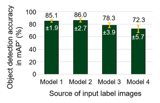
Figure 8.
Average and standard deviation of object detection accuracy of randomly chosen training and testing data, generated from input data of Models 1–4 in Table 2. * mAP: mean average precision (mAP) when intersect over union (IoU) is greater than 50%.
The decrease in mAP over time could be attributed to the fact that separation of individual plants becomes challenging as they grow (Figure 9). While their appearance in UAS images is generally uniform, and gaps between adjacent plants are well defined immediately after plant emergence, the gaps between individual plants tend to be covered by plant leaves over time, resulting in almost continuous canopy. At that point, it becomes difficult not only to delineate plant boundaries but also to determine the number of plants. Additionally, target objects located near the image boundary can cause inconsistency issues during labeling and training, since plants near the edge of an image may contain only partial coverage of the plant, therefore, and their shape might differ from intact plants found in the interior of the image. Furthermore, germination time and developmental phases vary within the field, due to microclimate or nutrition, resulting in variance of plant size.
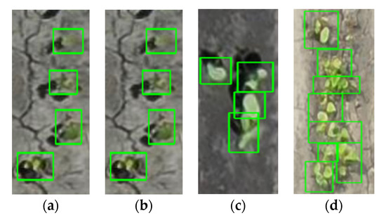
Figure 9.
Examples of manually labeled data on April (a) 15, (b) 16, (c) 18, and (d) 24. Note: These examples represent different locations of the experimental field with different zoom levels.
Even though care was taken to label images consistently, pinpointing the exact location and number of plants in the connected/clustered canopy area was challenging. Data shows that labeling performance in input training data, was adequate when there is good separation between plants, and then decreases in situations where plants are clustered or canopy overlaps (Figure 9). In cases where visual inspection fails to correctly label data, it may be unreasonable to expect that a machine learning model would outperform a human inference. In this regard, it seems that the timing of data acquisition will be very important for object detection-based plant counting. From the datasets of this study, 15 to 18 April (DAP 10 to 13) was effective to ensure object detection over 78% (Figure 8). It should be noted that the current dataset contains images of four different plant densities, from 3 to 12 plants per linear meter of row, and the effective period of UAS data can expand when the maximum plant density of target plot is lower than 12 plants per linear meter of row.
3.2. Object Detection Accuracy Using YOLOv3
When the training and testing images were both chosen from the corresponding dataset of the same flight, the mAP and F1 scores of the YOLOv3 model were higher than 78%, and 0.77, respectively, except for those derived from the 24 April data (Table 3). Training and testing data comprised of 15, 16, and 18 April, resulted in a higher accuracy, whether they were collected from a single date or multiple dates. In particular, it should be noted that the accuracy of Models 5 and 6 were comparable to that of Models 1 and 2. This suggests that a similar level of object detection accuracy can be achieved with an increased diversity in soil background, illumination, or plant shape in the training data.
Table 3.
YOLOv3 cotton detection models generated from different training and testing data.
The number of input training images used to train Models 1, 5, and 6 were 200, 400, and 600, and corresponding object detection accuracies were 88, 86, and 84%, when the models were applied to testing data of their own dates (left column in Table 3). It is expected that comparing the object detection accuracy of various YOLOv3 models, trained with training images in a 10–10,000 range, will clearly provide a more reliable guide to prepare an appropriate number of training datasets, however, more than 60 h will be required, only to label images, based on manual procedures, excluding model training and results interpretation. Although this paper does not rigorously investigate the effects of number of input data and plant detection accuracy, semi-automatic labeling methods based on Canopeo, and object detection algorithms, could help improve the efficiency of labelling, and investigate the effect of number of input training images.
As the reference plant count is available by 1 m2 for 15 April, the object detection performance of Models 1–10 was evaluated using the F1 score and mAP, when each model is tested on 15 April data. Models 1, 5, 6, and 7 contained 15 April images in their training sets, and these models showed a mAP over 80%. The highest accuracy was obtained from Model 1, which was assumed to be due to the consistency in training and testing data. A similar or slightly lower accuracy was observed from Models 5–7 that include training data of other dates. The mAP over 80% of Models 1, and 5–7, tested on 15 April data, indicates that detection accuracy can be maximized when training data include images of 15 April. Nevertheless, mAP declined from approximately 80% to 50% when 15 April images were not included in their training dataset. The models derived from single-date input (Models 2–4) exhibited an abrupt decrease in their accuracy. Model 4 for example was trained with 24 April data, and showed a mAP of 5.51% when tested on the 15 April data. It seems encouraging, however, that the use of multi-date labeled images as a training dataset could minimize the decrease of the detection accuracy. Within Models 5–10, mAP was greater than 53% when 15 April data were not used for training (Models 8–10), but mAP was above 79% when 15 April was used for training (Models 5–7). The usage of 15 April data in the training stage, and the use of multi-date labeled images, will affect final plant count results, therefore, this effect will also be discussed in Section 3.5.
Among the UAS data in this study, the background soil surface on 18 April was relatively darker, with less apparent soil crusting. Due to the difference in background brightness on that date, the YOLOv3 model performance was also evaluated. Similar to the previous results, models trained with 18 April data demonstrated higher accuracy when the models were applied to the testing data of 18 April. All models containing 18 April data in their training dataset showed mAP and F1 scores over 77%, and 0.70, respectively. On the contrary, mAP and F1 scores ranged between 43–67%, and 0.42–0.59, when training data did not contain the 18 April dataset. It is supposed that the combined effect of availability of 18 April training data, and the difference in background brightness, might have decreased the overall detection accuracy. However, Model 5 trained with multi-date labeled images, including 15 and 16 April, exhibited a higher detection mAP of 66%. It is considered that the low object detection accuracy, due to the absence of comparable training data, could be compensated by increasing the number of training data, even though the object or background information does not match well. Although reference plant count on 18 April is unavailable, the expected error of plant counting using Model 5 will be estimated in Section 3.5.
The mAP and F1 scores of YOLOv3 models on 15 and 18 April testing datasets, were mostly higher than 43% and 0.42. Although the 43–88% mAP achieved in this study appears low in comparison with a perfect detection rate of 100% mAP, the achieved value was higher than the mAP of other object detection algorithms, e.g., SSD, Faster R-CNN, and RetinaNet, that range between 28–38% [37]. It should be noted that, the object detection accuracy in mAP is not a measure of plant count error, and the final detection rate may increase by redundancy, created by multiple overlapping images. The overall trend between mAP and final plant count error will be discussed in Section 3.5.
The accuracy of object detection on 15 and 18 April testing data indicates that YOLOv3-based object detection performs adequately, even though differences in plant size, shape, or soil background exist in training and testing datasets. It was also shown that YOLOv3 models trained with multiple datasets exhibited stable performance, based on mAP and F1 score measures. However, it was evident that substantial differences of plant morphological appearance in training and testing data should be accounted for, to avoid a reduction in detection accuracy, such as noted for Model 4 on 15 April testing data.
3.3. Canopy and Non-Canopy Classification
The classification accuracy of canopy and non-canopy pixels is also important because the location of the plant center can be refined based on this result. Visual assessment of the Canopeo-based classification results was conducted by overlaying canopy pixels over the original RGB images (Figure 10). This revealed that nearly all plants with clear object boundaries were identified by the Canopeo algorithm, however, plants exhibiting off-green colors were rarely classified as canopy by the Canopeo algorithm. Unhealthy plants in the early season are unlikely to contribute to final crop yield, thus classifying such plants as non-canopy at this stage would be arguably inconsequential for the purpose of assessing plant population. In cases where there may be interest in identifying the plants with off-green color, such plants can be detected by a multi-class object detection approach, with an additional class of off-green plants supported by fine-tuning the of object center, using classification methods or thresholding of the excessive greenness index (ExG) image.
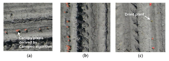
Figure 10.
Canopy pixels (red) overlaid on RGB images showing that (a–c) the majority of green plant pixels are correctly classified as canopy class by the Canopeo algorithm, whereas (c) off-green plants are not.
3.4. Determination of Optimal Parameters for Screening and Clustering Plant Centers
In an ideal case, plant centers obtained from multiple overlapping images should be projected on the exact geographic location of the plants, with minimal location error. However, errors in photogrammetric parameters (IO and EO) and the ground surface model can cause dispersion of projected centers, even though the errors were optimized by the SfM process (Figure 11b and Figure 12b). This study used a screening approach to reduce the number of plant centers that can induce larger dispersion of projection plant centers, and to find the best processing parameters that minimize error of plant count error.
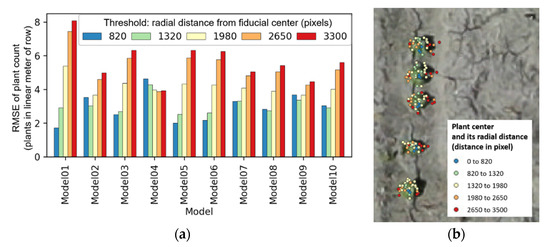
Figure 11.
Relation of radial distance threshold and average root mean square error (RMSE) of plant count (a); an example showing its effect on plant centers derived from Model 1 (b).
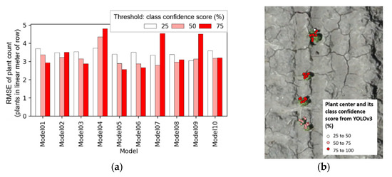
Figure 12.
Relation of class confidence threshold and average root mean square error (RMSE) of plant count (a); an example showing its effect on plant centers derived from Model 1 (b).
A small estimation error of the plant centers in the raw image space can be translated into a larger distance error in the projected geographic space, particularly when detected plants are far from the fiducial point. For this reason, radial distance threshold values of 820, 1320, 1980, 2650, and 3300 pixels, which is equivalent to 25%, 40%, 60%, 80%, and 100% of one-half diagonal pixel distance in the raw image, were used to filter out any points that are outside of the circular radius in the later stages. Another controlling parameter suggested here was the class confidence score from the YOLOv3 model. It was assumed that the dispersion in geographic space could be reduced by screening out plant centers with lower confidence scores. Threshold values used for class confidence scores were 25%, 50%, and 75%.
After screening plant centers using both criteria, an agglomerative clustering algorithm was applied to the chosen plant centers [51,52]. The clustering algorithm was tested by running it with 7 different threshold values of distance between clusters, i.e., 0.01, 0.02, 0.04, 0.05, 0.10, 0.15, and 0.20 m2. Afterwards, grid-wise plant counts were summarized for every combination of screening factor (radial distance and class confidence score), threshold of distance between two adjacent clusters (Equation (1)), and input YOLOv3 model (Table 3), and this resulted in a total of 1050 instances (5 cases from radial distance, 3 cases from class confidence score, 7 cases from distance measure in the clustering, and 10 YOLOv3 models: 5 × 3 × 7 × 10 = 1050). Root mean square error (RMSE) and R2, between manual and UAS-based counts, were calculated for each instance, to find optimal processing parameters.
Instances were separated into 5 groups according to the 5 radial distance threshold values for each model, and average RMSE was calculated. An average RMSE of 2.9, 3.0, 4.2, 5.3, and 5.6 plants, per linear meter of row, was observed, when radial distance was 820, 1320, 1980, 2650, and 3300. Figure 11a illustrates average RMSE, grouped by both radial distance threshold and the YOLOv3 models (Models 1–10). Projected ground centers tended to spread more widely when their image coordinates were far from the fiducial center (Figure 11b). Therefore, results with radial distance thresholds of 820, 1320, and 1980, which resulted in a total of 630 cases (3 cases from radial distance, 3 cases from class confidence score, 7 cases from distance measure, and 10 YOLOv3 models: 3 × 3 × 7 × 10 = 630), were used to identify the best performing parameters.
The 630 selected cases were separated into 3 groups by class confidence threshold of 25%, 50%, and 75%, and average RMSE was assessed for Models 1–10. When plant center coordinates were screened out by a 75% class confidence score, larger variances of average RMSE were observed, depending on which YOLOv3 model was used (Figure 12a). This could be because class confidence score can change abruptly when the appearance of the plant deviates from that of a well-separated single plant. For example, the upper three plants in Figure 12b show more concentrated canopy around the main stems, which was the common plant morphological appearance in 15 April data. Most of the plants showing the concentrated canopy structure had a class confidence score over 75%. On the contrary, the lowermost plant in the same figure (Figure 12b) showed two smaller canopy segments around its main stem, and its class confidence score was mostly 50–75%. There were many instances from the study area in which class confidence scores of valid plant centers were 25–75%. In this respect, cases with a class confidence score threshold of 25% or 50% were only used to minimize loss of input plant centers, resulting in 420 cases left in the search.
Average RMSE, according to the distance threshold between clusters, showed minor differences between input models, except when the threshold was 0.01 or 0.02 m2 (Figure 13a). It was also evident that the cluster distance threshold of 0.05 and 0.1 m2 produced smaller errors, when compared to others. Although the distance, defined by the Ward minimum variance method (Equation (1)), does not directly translate into a tangible distance concept, it is meaningful that the optimum range for this parameter could be identified. The effect of the cluster distance threshold on clustering results can be visually assessed in Figure 13b. The number of plants derived by the proposed clustering method, with the cluster distance threshold of 0.10 m2, perfectly matched the plant count driven by visual assessment (Figure 13b).
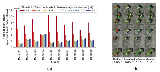
Figure 13.
Relation of cluster distance threshold and average root mean square error (RMSE) of plant count (a); an example showing its effect on agglomerative clustering when Model 1 was used (b).
The comparative analysis, between processing parameters and plant counting performance, revealed the applicable range of screening and clustering parameters. As one of the goals of this study is to suggest a plant counting procedure that works with general input UAS data, the average RMSE of plant count was assessed using Models 1–10, which were trained by different input training and testing datasets, and processing parameters with a minimum average RMSE were determined as optimal values. Average RMSE values derived from Models 1–10, when the selected screening and clustering parameters were applied, are shown in Table 4. The results indicate that average RMSE ranged from 1.02 to 2.83 plants per linear meter of row. The lowest average RMSE of Models 1–10 was 1.02 plants per linear meter of row, when class confidence score, radial distance, and cluster distance threshold were set to 25%, 1980 pixels, and 0.10 m2, respectively. It was considered that keeping a larger number of object centers, using a lower minimum class confidence score, was effective to minimize plant count error, when the distance threshold for clustering was 0.05 or 0.10 m2.
Table 4.
Average root mean square error (RMSE) of unmanned aircraft systems (UAS)-based plant count of Models 1 to 10 depending on different combination of screening and clustering parameters.
The three main hyperparameters used in the study should be adjusted when the proposed approach is applied with a different flight altitude, camera, or to a different target crop. Although in-depth investigation on hyperparameter tuning in different conditions was not conducted in this study, general recommendations can be drawn. Maximum radial distance from fiducial center is a parameter related to the quality of lens calibration, and should be decreased when poorly calibrated or a lower-quality lens is used. As the lens distortion error increases, smaller areas around the fiducial center will provide a reliable accuracy of image coordinates to ground surface projection. Minimum class confidence score is a parameter related to the quality of object detection results. A threshold value of 25% will be appropriate to minimize omission rate, when majority of detected objects have a smaller class confidence score due to small object size or diversity of object shape. However, a higher threshold value can be used if the target object is more distinctive, and the resultant class confidence score is generally higher. Maximum distance between adjacent clusters should be determined considering the ground projection errors. The location accuracy of the projected plant center can improve as flight altitude is lowered, or target plants are more regularly shaped, therefore, a smaller value for this parameter can be used.
3.5. Accuracy of Plant Counting
Assuming the average error was optimized with the steps discussed previously, RMSE and R2 values for Models 1–10 were examined (Table 5). The majority of RMSE and R2 values ranged between 0.50–1.14 plants per linear meter of row, and 0.82–0.97, respectively, and Models 1, 3, 5, 6, 7, and 8 showed optimal results with RMSE values ranging from 0.50 to 0.85 plants per linear meter of row. It should be noted that the RMSE values of multiple-date inputs (Models 5–10) were generally smaller than those of single-date input models (Models 1–4), as a similar trend was shown from the object detection accuracy (Figure 14). Therefore, it is considered that the accuracy of the deep learning-based plant counting method can be improved by including training data containing variability of plant size, shape, and background information for practical applications.
Table 5.
RMSE and R2 of UAS-based plant counting when class confidence score, maximum radial distance, and cluster distance threshold were set to 25%, 1980 pixels, and 0.10 m2, respectively.
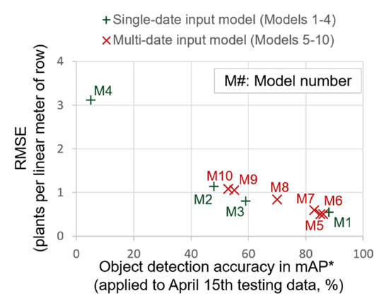
Figure 14.
Relation of plant count error and object detection accuracy depending on the use of single-date or multi-date input training data. The plant count errors in RMSE were obtained by applying the proposed plant counting method when class confidence, maximum radial distance, and cluster distance threshold were 25%, 1980 pixels, and 0.10 m2. * mAP: mean average precision (mAP) when intersect over union (IoU) is greater than 50%.
However, Model 4 (trained with 24 April data) resulted in an extremely large error of 3.11 plants per linear meter of row (Table 5), and Models 9 and 10, which used 24 April data during training, also produced slightly higher RMSE values of 1.06 and 1.09 plants per meter of row. The higher RMSE from Models 4, 9, and 10 can be largely attributed to differences in the morphological plant characteristics in the training and test datasets, as previously discussed.
Except for the results derived from Model 4, the RMSE of plant count of 0.50–1.14 plants per linear meter of row was achieved from all other YOLOv3 models, when mAP was over 45% (Figure 14). From inverse correlation between object detection accuracy and RMSE of plant count, it can also be presumed that expected values of plant count error (RMSE) is 0.5–1.2 when object detection accuracy (mAP) is 50–90%, and RMSE of plant count becomes lower than 1.0 when object detection accuracy is over 80%.
The range of RMSE when 15 April data were used in the training (Model 1 and 5–7) and when 15 April data were not used in the training (Models 2, 3, and 8), was 0.50–0.60, and 0.81–1.14 plants per linear meter of row. Therefore, it should be restated that training data should be collected from at least two different dates to obtain optimal results using the proposed method. In the following paragraphs, best results derived from two YOLOv3 models trained with 15 April data (Models 1 and 5), and a model trained without (Models 3), are presented to discuss the effect of availability of training data acquired from the date of inference (15 April).
From the plant count results in Table 5, Models 1, 5, 6, and 7 were considered effective based on the lower RMSE, ranging from 0.50 to 0.60 plants per linear meter of row. Figure 15a–d shows a scatter plot between the reference plant count and the optimal UAS-based plant count, derived from Models 1 and 5. Although Model 5 resulted in the lowest RMSE, Models 1, 6, and 7 also produced almost identical trends, as shown in Figure 15a. When assessing the relationship between the reference plant count and the UAS-based plant count, it was evident that most of the data points were distributed along the 1:1 line on the scatter plot (Figure 15a,c) when plant density was 0–14 plants per linear meter of row. Previous research indicates that yield potential can be drastically reduced when the number of plants per linear meter of row is below five plants per linear meter of row [5]. It is encouraging, since the proposed methodology performs well under these conditions, improving the chances of identifying areas prone to yield penalties due to inadequate plant population. For 82% of all 1 m2 grids, reference and UAS-based plant counts were identical, and 99% of the estimates showed an absolute error of less than or equal to two (Figure 15b,d).
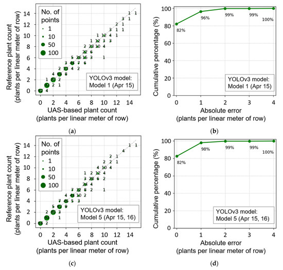
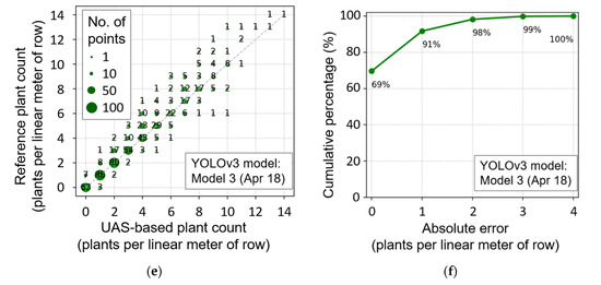
Figure 15.
Comparison of a unmanned aircraft systems (UAS)-based plant count with reference plant count measurement (a,c,e), and cumulative percentage of plants, according to absolute count error (b,d,f) when Model 1 (a,b), Model 5 (c,d), and Model 3 (e,f) were used.
Nevertheless, the accuracy of the proposed method was lower when reference plant count was greater than 10 plants per linear meter of row, based on the ratio of correct and incorrect results (Figure 15a,c). A larger variance in this region can be associated with the increase in canopy overlap, as well as the limited number of input data points (i.e., the less frequent appearance in the training data, Figure 1b). In order to overcome this problem with the object detection approach, more data is required, with plant count, greater than, or equal to, 10. Alternatively, a more sophisticated process, exploiting detailed object skeletal structure [25] or a feature extraction and classification method [23], can be performed to determine the exact number of plants and their locations.
The best plant count results without 15 April training data were achieved by Model 3. Although data are generally distributed around 1:1 line, larger variance was observed throughout the entire range, with a slight underestimating trend (Figure 15e). This result indicates the necessity of training data of earlier dates, when plants do not severely overlap each other, and the effectiveness of multi-date training data, to obtain a lower RMSE of plant count in the cotton seedling stage.
The implementation of proposed method, with diverse input training data and appropriate set of hyperparameters, resulted in a RMSE of plant counting less than 0.6 in the initial growth stages of cotton. While this study focuses on optimizing the three major hyperparameters (class confidence score, maximum radial distance, and cluster distance threshold) to minimize the RMSE of plant count, use of a novel object detection algorithm that is capable of detecting small objects and separating overlapping objects will greatly improve the performance of image-based plant counting.
3.6. Processign Time
The UAS-based stand counting process was performed on Dell compute nodes, with Intel Xeon processors and Nvidia Tesla GPUs (either 2 P100 or 2 V100). Table 6 shows approximate processing time of the research method on the study area of 400 m2. Total estimated time required for the entire procedure was 489 min, when pre-trained YOLOv3 model was unavailable. However, the time required for labeling data (120 min) and training the YOLOv3 network (300 min) could be saved in the case that a pre-trained YOLOv3 model exists, resulting in a processing time of 69 min for this case. Although the UAS used in this study did not have the capability of accurate measurement of camera location, use of UAS with RTK GPS technology could reduce by an additional 30 min the SfM process and ground surface model generation, allowing pseudo real-time processing of the overall procedure in 30 min.
Table 6.
Estimated processing time of the proposed approach in a 40 m by 10 m area.
4. Conclusions
In this study, we proposed a framework for cotton plant counting using the YOLOv3 object detection model, leveraging high resolution UAS imagery. In essence, this paper discusses UAS data collection configuration, plant counting procedure, and the evaluation of plant count results.
The proposed plant counting procedure consists of 3 steps: (1) ground surface generation, (2) YOLOv3 object detection, and (3) image coordinates to ground surface projection and clustering. The proposed approach performs object detection from raw UAS images, which enables object detection in the original image resolution (GSD). The object localization procedure, using camera locations and poses (EO), provides not only the exact geographic coordinate of detected objects but also multiple attempts for object detection. The accuracy of the plant counting algorithm was optimized by three processing parameters, i.e., radial distance from fiducial center to object center, class confidence score, and cluster distance thresholds. One of the advantages of the proposed method is that only three parameters determine the quality of the plant count results, and optimal ranges of the three parameters were identified as 820–1980 pixels for the radial distance, 25–50% for class confidence score, and 0.05–0.10 m2 for the cluster distance threshold.
The RMSE and R2 values of the YOLOv3-based input models ranged from 0.50 to 0.60 plants per linear meter of row, and 0.96 to 0.97, respectively. Six out of 10 models exhibited a RMSE ranging between 0.50 and 0.85 plants per linear meter of row. Models trained by multiple UAS data showed more stable results when compared to those driven by single-date training data input. The proposed method generally performed well when plant population ranges were between 0 and 14 plants per linear meter of row, and when plants were generally separable from each other. In order to increase the reliability of the proposed approach to severely overlapping plants, a novel object detection algorithm that is capable of detecting small objects and separating overlapping objects could be used instead of the YOLOv3 algorithm. The proposed framework can potentially be implemented to generate actionable, and timely, information that will aid the decision-making process at the farm level.
Author Contributions
Conceptualization, J.J., S.O., and J.L.; methodology, S.O. and J.J., and A.C.; software, S.O.; validation, S.O., J.J., and N.D.; formal analysis, S.O. and J.J.; investigation, S.O. and J.J.; resources, D.G., N.D., A.A., and J.L.; data curation, S.O., N.D., A.A., and A.C.; writing—original draft preparation, S.O.; writing—review and editing, J.J., M.M., A.C., N.D., and A.A.; visualization, S.O. and J.J.; supervision, J.J.; project administration, J.J. and J.L.; funding acquisition, J.J. and J.L. All authors have read and agreed to the published version of the manuscript.
Funding
This research was funded by Texas A&M AgriLife Research.
Acknowledgments
This work was supported by Texas A&M AgriLife Research.
Conflicts of Interest
The authors declare no conflict of interest.
References
- Reddy, K.R.; Reddy, V.R.; Hodges, H.F. Temperature effects on early season cotton growth and development. Agron. J. 1992, 84, 229–237. [Google Scholar] [CrossRef]
- Reddy, K.R.; Brand, D.; Wijewardana, C.; Gao, W. Temperature effects on cotton seedling emergence, growth, and development. Agron. J. 2017, 109, 1379–1387. [Google Scholar] [CrossRef]
- Briddon, R.W.; Markham, P.G. Cotton leaf curl virus disease. Virus Res. 2000, 71, 151–159. [Google Scholar] [CrossRef]
- Wheeler, T.R.; Craufurd, P.Q.; Ellis, R.H.; Porter, J.R.; Vara Prasad, P.V. Temperature variability and the yield of annual crops. Agric. Ecosyst. Environ. 2000, 82, 159–167. [Google Scholar] [CrossRef]
- Hopper, N.; Supak, J.; Kaufman, H. Evaluation of several fungicides on seedling emergence and stand establishment of Texas high plains cotton. In Proceedings of the Beltwide Cotton Production Research Conference, New Orleans, LA, USA, 5–8 January 1988. [Google Scholar]
- Wrather, J.A.; Phipps, B.J.; Stevens, W.E.; Phillips, A.S.; Vories, E.D. Cotton planting date and plant population effects on yield and fiber quality in the Mississippi Delta. J. Cotton Sci. 2008, 12, 1–7. [Google Scholar]
- UC IPM Pest Management Guidelines: Cotton. Available online: http://ipm.ucanr.edu/PDF/PMG/pmgcotton.pdf (accessed on 3 July 2020).
- Hunt, E.R.; Daughtry, C.S.T. What good are unmanned aircraft systems for agricultural remote sensing and precision agriculture? Int. J. Remote Sens. 2018, 39, 5345–5376. [Google Scholar] [CrossRef]
- Chang, A.; Jung, J.; Maeda, M.M.; Landivar, J. Crop height monitoring with digital imagery from Unmanned Aerial System (UAS). Comput. Electron. Agric. 2017, 141, 232–237. [Google Scholar] [CrossRef]
- Roth, L.; Streit, B. Predicting cover crop biomass by lightweight UAS-based RGB and NIR photography: An applied photogrammetric approach. Precis. Agric. 2018, 19, 93–114. [Google Scholar] [CrossRef]
- Maimaitijiang, M.; Ghulam, A.; Sidike, P.; Hartling, S.; Maimaitiyiming, M.; Peterson, K.; Shavers, E.; Fishman, J.; Peterson, J.; Kadam, S.; et al. Unmanned Aerial System (UAS)-based phenotyping of soybean using multi-sensor data fusion and extreme learning machine. ISPRS J. Photogramm. Remote Sens. 2017, 134, 43–58. [Google Scholar] [CrossRef]
- Berni, J.A.J.; Zarco-Tejada, P.J.; Suárez, L.; Fereres, E. Thermal and narrowband multispectral remote sensing for vegetation monitoring from an unmanned aerial vehicle. IEEE Trans. Geosci. Remote Sens. 2009, 47, 722–738. [Google Scholar] [CrossRef]
- Duan, T.; Zheng, B.; Guo, W.; Ninomiya, S.; Guo, Y.; Chapman, S.C. Comparison of ground cover estimates from experiment plots in cotton, sorghum and sugarcane based on images and ortho-mosaics captured by UAV. Funct. Plant Biol. 2017, 44, 169–183. [Google Scholar] [CrossRef]
- Jung, J.; Maeda, M.; Chang, A.; Landivar, J.; Yeom, J.; McGinty, J. Unmanned aerial system assisted framework for the selection of high yielding cotton genotypes. Comput. Electron. Agric. 2018, 152, 74–81. [Google Scholar] [CrossRef]
- Ashapure, A.; Jung, J.; Yeom, J.; Chang, A.; Maeda, M.; Maeda, A.; Landivar, J. A novel framework to detect conventional tillage and no-tillage cropping system effect on cotton growth and development using multi-temporal UAS data. ISPRS J. Photogramm. Remote Sens. 2019, 152, 49–64. [Google Scholar] [CrossRef]
- Chen, A.; Orlov-Levin, V.; Meron, M. Applying high-resolution visible-channel aerial imaging of crop canopy to precision irrigation management. Agric. Water Manag. 2019, 216, 196–205. [Google Scholar] [CrossRef]
- Huang, H.; Deng, J.; Lan, Y.; Yang, A.; Deng, X.; Zhang, L.; Wen, S.; Jiang, Y.; Suo, G.; Chen, P. A two-stage classification approach for the detection of spider mite- infested cotton using UAV multispectral imagery. Remote Sens. Lett. 2018, 9, 933–941. [Google Scholar] [CrossRef]
- Wang, T.; Alex Thomasson, J.; Yang, C.; Isakeit, T. Field-region and plant-level classification of cotton root rot based on UAV remote sensing. In Proceedings of the 2019 ASABE Annual International Meeting, Boston, MA, USA, 7–10 July 2019. [Google Scholar]
- Yeom, J.; Jung, J.; Chang, A.; Maeda, M.; Landivar, J. Automated open cotton boll detection for yield estimation using unmanned aircraft vehicle (UAV) data. Remote Sens. 2018, 10, 1895. [Google Scholar] [CrossRef]
- Ehsani, R.; Wulfsohn, D.; Das, J.; Lagos, I.Z. Yield estimation: A low-hanging fruit for application of small UAS. Resour. Eng. Technol. Sustain. World 2016, 23, 16–18. [Google Scholar]
- Chen, R.; Chu, T.; Landivar, J.A.; Yang, C.; Maeda, M.M. Monitoring cotton (Gossypium hirsutum L.) germination using ultrahigh-resolution UAS images. Precis. Agric. 2018, 19, 161–177. [Google Scholar] [CrossRef]
- Feng, A.; Sudduth, K.A.; Vories, E.D.; Zhou, J. Evaluation of cotton stand count using UAV-based hyperspectral imagery. In Proceedings of the 2019 ASABE Annual International Meeting, Boston, MA, USA, 7–10 July 2019. [Google Scholar]
- Jin, X.; Liu, S.; Baret, F.; Hemerlé, M.; Comar, A. Estimates of plant density of wheat crops at emergence from very low altitude UAV imagery. Remote Sens. Environ. 2017, 198, 105–114. [Google Scholar] [CrossRef]
- Gnädinger, F.; Schmidhalter, U. Digital counts of maize plants by unmanned aerial vehicles (UAVs). Remote Sens. 2017, 9, 544. [Google Scholar] [CrossRef]
- Liu, T.; Wu, W.; Chen, W.; Sun, C.; Zhu, X.; Guo, W. Automated image-processing for counting seedlings in a wheat field. Precis. Agric. 2016, 17, 392–406. [Google Scholar] [CrossRef]
- Kalantar, B.; Mansor, S.B.; Shafri, H.Z.M.; Halin, A.A. Integration of template matching and object-based image analysis for semi-Automatic oil palm tree counting in UAV images. In Proceedings of the 37th Asian Conference on Remote Sensing, ACRS 2016, Colombo, Sri Lanka, 17–21 October 2016. [Google Scholar]
- Salamí, E.; Gallardo, A.; Skorobogatov, G.; Barrado, C. On-the-Fly Olive Tree Counting Using a UAS and Cloud Services. Remote Sens. 2019, 11, 316. [Google Scholar] [CrossRef]
- Gu, J.; Grybas, H.; Congalton, R.G. Individual Tree Crown Delineation from UAS Imagery Based on Region Growing and Growth Space Considerations. Remote Sens. 2020, 12, 2363. [Google Scholar] [CrossRef]
- De Castro, A.I.; Torres-Sánchez, J.; Peña, J.M.; Jiménez-Brenes, F.M.; Csillik, O.; López-Granados, F. An Automatic Random Forest-OBIA Algorithm for Early Weed Mapping between and within Crop Rows Using UAV Imagery. Remote Sens. 2018, 10, 285. [Google Scholar] [CrossRef]
- Wetz, M.S.; Hayes, K.C.; Fisher, K.V.B.; Price, L.; Sterba-Boatwright, B. Water quality dynamics in an urbanizing subtropical estuary (Oso Bay, Texas). Mar. Pollut. Bull. 2016, 104, 44–53. [Google Scholar] [CrossRef]
- Schonberger, J.L.; Frahm, J.M. Structure-from-Motion Revisited. In Proceedings of the IEEE Computer Society Conference on Computer Vision and Pattern Recognition, Las Vegas, NV, USA, 27–30 June 2016. [Google Scholar]
- Westoby, M.J.; Brasington, J.; Glasser, N.F.; Hambrey, M.J.; Reynolds, J.M. “Structure-from-Motion” photogrammetry: A low-cost, effective tool for geoscience applications. Geomorphology 2012, 179, 300–314. [Google Scholar] [CrossRef]
- Lowe, D.G. Distinctive image features from scale-invariant keypoints. Int. J. Comput. Vis. 2004, 60, 91–110. [Google Scholar] [CrossRef]
- Hess, M.; Green, S. Structure from motion. In Digital Techniques for Documenting and Preserving Cultural Heritage; Bentkowska-Kafel, A., MacDonald, L., Eds.; Arc Humanities Press: York, UK, 2017; pp. 243–246. [Google Scholar]
- Furukawa, Y.; Ponce, J. Accurate, dense, and robust multiview stereopsis. IEEE Trans. Pattern Anal. Mach. Intell. 2010, 32, 1362–1376. [Google Scholar] [CrossRef]
- Haala, N.; Rothermel, M. Dense multi-stereo matching for high quality digital elevation models. Photogramm. Fernerkund. Geoinf. 2012, 2012, 331–343. [Google Scholar] [CrossRef]
- YOLOv3: An Incremental Improvement. Available online: https://pjreddie.com/media/files/papers/YOLOv3.pdf (accessed on 3 July 2020).
- Redmon, J.; Farhadi, A. YOLO9000: Better, faster, stronger. In Proceedings of the 30th IEEE Conference on Computer Vision and Pattern Recognition, CVPR 2017, Honolulu, HI, USA, 21–26 July 2017. [Google Scholar]
- Tong, K.; Wu, Y.; Zhou, F. Recent advances in small object detection based on deep learning: A review. Image Vis. Comput. 2020, 97, 103910. [Google Scholar] [CrossRef]
- Torralba, A.; Fergus, R.; Freeman, W.T. 80 million tiny images: A large data set for nonparametric object and scene recognition. IEEE Trans. Pattern Anal. Mach. Intell. 2008, 30, 1958–1970. [Google Scholar] [CrossRef] [PubMed]
- Pedregosa, F.; Varoquaux, G.; Gramfort, A.; Michel, V.; Thirion, B.; Grisel, O.; Blondel, M.; Prettenhofer, P.; Weiss, R.; Dubourg, V.; et al. Scikit-learn: Machine learning in Python. J. Mach. Learn. Res. 2011, 12, 2826–2830. [Google Scholar]
- Varoquaux, G.; Buitinck, L.; Louppe, G.; Grisel, O.; Pedregosa, F.; Mueller, A. Scikit-learn. GetMobile Mob. Comput. Commun. 2015, 19. [Google Scholar] [CrossRef]
- Patrignani, A.; Ochsner, T.E. Canopeo: A powerful new tool for measuring fractional green canopy cover. Agron. J. 2015, 107, 2312–2320. [Google Scholar] [CrossRef]
- Chung, Y.S.; Choi, S.C.; Silva, R.R.; Kang, J.W.; Eom, J.H.; Kim, C. Case study: Estimation of sorghum biomass using digital image analysis with Canopeo. Biomass Bioenerg. 2017, 105, 207–210. [Google Scholar] [CrossRef]
- Di Stefano, L.; Bulgarelli, A. A simple and efficient connected components labeling algorithm. In Proceedings of the 10th International Conference on Image Analysis and Processing, Venice, Italy, 27–29 September 1999. [Google Scholar]
- Image Processing Review, Neighbors, Connected Components, and Distance. Available online: http://homepages.inf.ed.ac.uk/rbf/CVonline/LOCAL_COPIES/MORSE/connectivity.pdf (accessed on 3 July 2020).
- Enciso, J.M.; Colaizzi, P.D.; Multer, W.L. Economic analysis of subsurface drip irrigation lateral spacing and installation depth for cotton. Trans. Am. Soc. Agric. Eng. 2005, 48, 197–204. [Google Scholar] [CrossRef]
- Khan, N.; Usman, K.; Yazdan, F.; Din, S.U.; Gull, S.; Khan, S. Impact of tillage and intra-row spacing on cotton yield and quality in wheat–cotton system. Arch. Agron. Soil Sci. 2015, 61, 581–597. [Google Scholar] [CrossRef]
- Yazgi, A.; Degirmencioglu, A. Optimisation of the seed spacing uniformity performance of a vacuum-type precision seeder using response surface methodology. Biosyst. Eng. 2007, 97, 347–356. [Google Scholar] [CrossRef]
- Nichols, S.P.; Snipes, C.E.; Jones, M.A. Cotton growth, lint yield, and fiber quality as affected by row spacing and cultivar. J. Cotton Sci. 2004, 8, 1–12. [Google Scholar]
- Murtagh, F.; Legendre, P. Ward’s Hierarchical Agglomerative Clustering Method: Which Algorithms Implement Ward’s Criterion? J. Classif. 2014, 31, 274–295. [Google Scholar] [CrossRef]
- Bouguettaya, A.; Yu, Q.; Liu, X.; Zhou, X.; Song, A. Efficient agglomerative hierarchical clustering. Expert Syst. Appl. 2015, 42, 2785–2797. [Google Scholar] [CrossRef]
© 2020 by the authors. Licensee MDPI, Basel, Switzerland. This article is an open access article distributed under the terms and conditions of the Creative Commons Attribution (CC BY) license (http://creativecommons.org/licenses/by/4.0/).