SLRL4D: Joint Restoration of Subspace Low-Rank Learning and Non-Local 4-D Transform Filtering for Hyperspectral Image

Abstract

During the process of signal sampling and digital imaging, hyperspectral images (HSI) inevitably suffer from the contamination of mixed noises. The fidelity and efficiency of subsequent applications are considerably reduced along with this degradation. Recently, as a formidable implement for image processing, low-rank regularization has been widely extended to the restoration of HSI. Meanwhile, further exploration of the non-local self-similarity of low-rank images are proven useful in exploiting the spatial redundancy of HSI. Better preservation of spatial-spectral features is achieved under both low-rank and non-local regularizations. However, existing methods generally regularize the original space of HSI, the exploration of the intrinsic properties in subspace, which leads to better denoising performance, is relatively rare. To address these challenges, a joint method of subspace low-rank learning and non-local 4-d transform filtering, named SLRL4D, is put forward for HSI restoration. Technically, the original HSI is projected into a low-dimensional subspace. Then, both spectral and spatial correlations are explored simultaneously by imposing low-rank learning and non-local 4-d transform filtering on the subspace. The alternating direction method of multipliers-based algorithm is designed to solve the formulated convex signal-noise isolation problem. Finally, experiments on multiple datasets are conducted to illustrate the accuracy and efficiency of SLRL4D.

1. Introduction

It began with the forging of the great imaging spectrometer. Many merits were given to the generated hyperspectral image (HSI)—multi bands, high resolution and rich details [1]. The vision of mankind was no longer merely limited to the spatial dimension with the assistance of HSI. An increasing number of application fields now rely on HSI, for instance, urban planning, geological exploration, military surveillance and precision agriculture [2]. Among these application fields, many critical tasks of computer vision processing such as unmixing [3], target detection [4], and classification [5] demand extremely high data quality. However, during sampling and acquisition, HSI is constantly degraded by mixed noises, for example, Gaussian noise, impulse noise, stripes and deadlines [6]. Under these circumstances, the accuracy and efficiency of the above work will be badly weakened. Therefore, as a key pre-processing step in HSI processing, the design of the restoration methodology has been an extremely valuable, active and high-interest research topic in recent years.

The general idea of traditional HSI restoration methods is to extend the band-by-band or pixel-by-pixel methods that are applied to gray images. The disadvantage of these methods is distinct; that is, the spatial or spectral correlations of the 3-D HSI are not maintained. Although methods based on wavelet shrinkage [7,8,9], non-local means [10], sparse representation [11,12,13,14] or deep learning [15,16,17,18,19] achieve the combination of spatial-spectral information, the sphere of their application is still limited. The prior knowledge of the original image and mixed noises are insufficiently explored and usually remove specific noise only; thus, their performance in real scenarios is not guaranteed.

1.1. Restoration by Low-Rank Property

Inspired by the robust principal component analysis model (RPCA) [20], He et al. conducted research to explore the low-rank property of HSI and modelled the HSI restoration as a low-rank matrix recovery (LRMR) problem, thus realizing the removal of various mixed noises [21]. This work proved that the probability is extremely high of restoring the low-rank latent clean HSI matrix from the observation HSI matrix, which is degraded by mixed noises. During the process of restoration, performance would be much improved if the global and local redundancies of HSI were both thoroughly utilized [22]. In Reference [23], a sparse method is employed to encode the global and local redundancy of the spectral dimension. Meanwhile, the global redundancy of the spectral dimension is explored by a low-rank constraint. Chen et al. [24] proposed a low-rank non-negative matrix factorization method to capture the spectral geometric features while maximizing the restoration of spatial detail. However, the spatial smoothing information of HSI is not fully utilized by the studies above. Due to the powerful ability to maintain the spatial smoothness of the image, the total variation (TV) regularized low-rank methods [25] are widely used in HSI restoration research. Aggarwal et al. [26] extended the traditional TV model to the three-dimensional space, and proposed a spatio-spectral total variation (SSTV) method for HSI restoration. The proposed SSTV method considers the high correlations in both the spatial and spectral dimensions, and performance enhancement of the TV-based restoration is achieved. However, in SSTV, only local spatial and spectral features have been explored. There is still no further research on the global low-rank property of HSI. Based on LRMR, Wang et al. continued their previous research [27] and proposed a combinatorial method with low-rank constraints named LSSTV [28]. The HSI restoration problem is modelled as a weighted nuclear norm minimization problem, and the jagged distortion left in SSTV is solved under certain circumstances. As an improvement of the LRMR, He et al. designed a TV regularized low-rank factorization method [29]. For further enhancement, they divided the HSI cube into many local patches, then imposed low-rank constraints on these patches [30]. This is about images in local fields have a high probability of containing the same features, thus, they usually share similar spectral features [31]. Tensor representation methods also shows great potential to explore the low-rank property [32]. Fan et al. extended the low-rank constraints to tensor represented HSI, and proposed a low-rank tensor recovery method that maintains correlations between three dimensions of HSI [33]. Wang et al. [34] combined tensor Tucker decomposition and anisotropic spatial-spectral TV, achieving exciting results in the removal of mixed noises.

However, the lack of spatial information often leads to poor restoration performance when strong Gaussian noise arrives. Most of the low-rank methods above only consider the piecewise smoothness or local similarity of the spatial dimension. Meanwhile, TV-based methods often cause distortion in the spectral domain, and some noises also appear smooth property (e.g., white Gaussian noise) [35]. The structural information of restored HSI is not guaranteed in these methods.

1.2. Restoration by Non-Local Similarity

Non-local self-similarity (NSS) theory holds that a patch of an image has many homogeneous patches with similar characteristics at other positions of the image. Since the structure of the clean image is redundant, similar patches of the target patch may exist at any position [36]. The NSS-based restoration method exploits this information redundancy of HSI to get rid of noises, where details of the spatial domain are kept to the greatest extent in course of denoising [37]. The priors of low-rankness and NSS are bonded in Reference [38]. By imposing non-local priors to the LRMR model, both pixels and spectrum in HSI are double corrected to remove mixed noises while preserving the fine spatial structure of HSI, thus improving the denoising performance. Bai et al. [39] applied a fixed window to extract non-local patches from the original image, and characterized the non-local similarity of HSI in the spatial domain and the global similarity in the spectral domain. In Reference [40], Xue et al. embedded the combined prior terms of low-rank and NSS into a sparse representation model. For further research, the tensor CANDECOMP/PARAFAC (CP) decomposition is applied to the joint denoising model [41]. Under this circumstance, the spatial information, for instance, image edges and textures of HSI, was further exploited, and the low-rank property was further utilized by the clustering of non-local patches. Both the global correlation along the spectrum and NSS were explored by Xie et al. [42]. In this work, all non-local patches were stacked to a third-order tensor and achieved excellent denoising performance. Similar research has been conducted in Reference [43]; the group sparsity and low-rank property of HSI are further utilized. Zhang et al. hypothesized that the piecewise smooth feature exists in the restored non-local patches of HSI, and thus conducted research on the combination of NSS and TV [44]. Considering the poor maintenance of CP decomposition on the intrinsic structure of HSI, Chen et al. applied a novel tensor decomposition approach named tensor ring decomposition to the non-local based HSI restoration model [45].

Unfortunately, although NSS-based low-rank methods have delivered gratifying restoration performance, the setting of certain parameters impacts the result of restoration excessively. For instance, various sizes of the search window and number of non-local patches often bring different results, some of which are unacceptable. Maggioni et al. designed a block-matching and 4D filtering (BM4D) restoration algorithm, which extended planar space denoising to three-dimensional space, and provided new ideas for HSI restoration [46,47]. This work simultaneously exploits the local correlation and non-local correlation between voxels instead of pixels, high-dimensional data is thus divided into many patches with similar features. Then, these patches are stacked together to form a four-dimensional hyperrectangle. Eventually, two diverse steps of estimation occur, the signal and noise are isolated by order of thresholding or Wiener filtering. The best legacy of this work is that actual parameter-free denoising is accomplished when applying BM4D to the HSI restoration problem. However, as with all NSS based restoration methods, the processing procedure of BM4D is relatively intricate, which ineluctably results in excessive time consumption when confronting the huge size of the original image space of HSI.

1.3. Restoration by Subspace Projection

Recently, the subspace low-rank (SLR) representation method has shown great potential to address the above challenges [48,49,50,51,52]. The theory of manifold learning suggests that the data in high-dimensional space is immoderately redundant, and principal information lives in the low-dimensional subspace [53]. Similar theories exist in the HSI compression field. Since the high-dimensional data is redundant, according to the low-rank property of HSI, the dimensions of the dictionary matrix and coefficient matrix generated from the low-rank decomposition are necessarily much lower than the dimension of the original image, thereby the purpose of data compression is realized. The reconstruction process is the inverse of compression, that is, the linear combination of dictionary and coefficient is the original image. Therefore, through this low-rank decomposition method, it is no longer necessary to store the original high-dimensional data, but only the compressed low-dimensional data. For low-rank image restoration, Figure 1 illustrates the distribution of singular value in the original space and low-dimensional subspace of the HYDICE Urban dataset. Since the spectrum of HSI lives in the low-dimensional subspace, as shown in Figure 1, the subspace has a lower singular value than the original space, which indicates that the subspace decomposition can yield a more accurate low-rank approximation. Part of this subspace low-rank property is given by the lower dimension of the projected matrix, and the other is given by the finiteness of the linear combination of end-members. For any pixel in HSI, it is impossible to be mixed by all end-members in the scene, but only a few of them (usually 2–3 end-members). This sparsity of the linear combination of end-members leads to the low-rankness of the decomposed coefficient matrix. Therefore, through imposing low-rank regularization to the subspace of HSI instead of the original space, better restoration results would be achieved. Reference [49] fused spectral subspace low-rank learning and superpixel segment, its restoration results proved that subspace does carry stronger low-rank property. By taking advantage of the subspace decomposition, a fast restoration method through using denoiser on subspace is proposed in [50] , but the fixed subspace basis they used also prevents the further rising of restoration results. References [48,51] proposed a Gaussian noise-removal method by combining low-rank subspace decomposition and weighted nuclear norm minimum, and achieved outstanding results. However, this advancement comes with the reduction of usability, as complex parameter settings greatly suppress the real application. Reference [52] modeled mixed denoising problem with a robust $l_1$ norm, and achieved the unification of complex statistical noise distribution. The number of parameters that need to be manually tuned is reduced, thus its usability and efficiency in real application is further enhanced. However, these studies also show that along with low-rank-based restoration methods, SLR-based methods are also powerless when encountering structured sparse noise and strong Gaussian noise. It is essential to further exploit the high correlation in the spatial dimension of HSI by exploring the NSS prior based on SLR. Meanwhile, the complexity of the parameters should be as simple as possible to make the proposed method easier to be implement. Through the discreet design of a low-dimensional orthogonal dictionary and prior regularization, the joint method of SLR and NSS not only accomplishes precise restoration of HSI, but also reduces the cost of computation. In this way, the NSS property is utilized in subspace, the dilemma of heavy computation cost of NSS-based methods is distinctly compensated.

In this paper, a joint method of subspace low-rank learning and non-local 4-D transform filtering, named SLRL4D, is presented for HSI restoration. By assuming that the latent clean HSI exists in the low-dimensional subspace, the NSS prior of the HSI is embedded into the SLR learning architecture. Thus, the high correlation of HSI in both spatial and spectral dimensions is thoroughly explored, and the successful removal of the mixed noises of HSI is realized. The main contributions of this paper are summarized as:

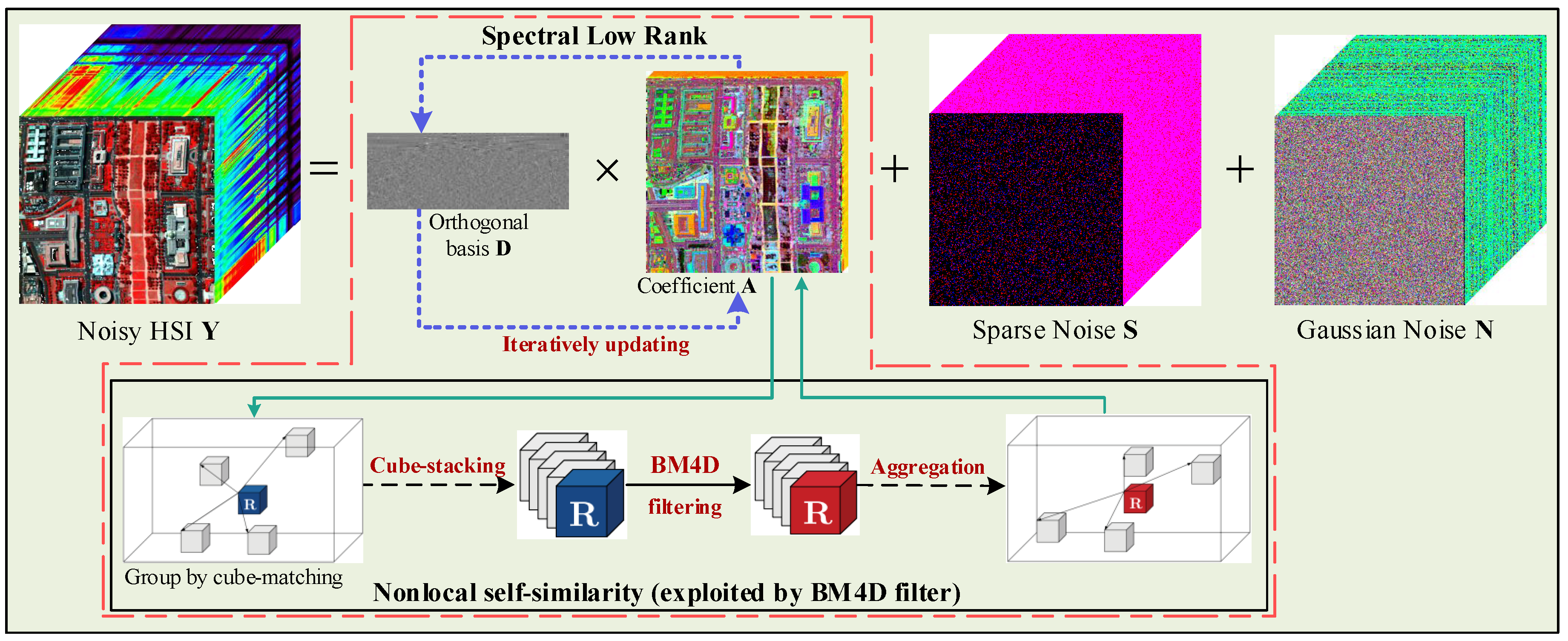
• The subspace low-rank learning method is designed to restore the clean HSI from the contaminated HSI which is degraded by mixed noises. An orthogonal dictionary with far lower dimensions is learned during the process of alternating updates, thus leading to precise restoration of the clean principal signal of HSI.
• Based on the full exploration of low-rank property in subspace, BM4D filtering is employed to further explore the NSS property within the subspace of HSI rather than the original space. By preserving the details of the spatial domain more precisely, the complete parameter-free BM4D filtering leads to easier application in real world.
• Each term in the proposed restoration model is convex after careful design, thus, the convex optimization algorithm based on the alternating direction method of multipliers (ADMM) could be derived to solve and optimize this model. Meanwhile, due to the HSI being decomposed into two sub-matrices of lower dimensions, computational consumption of the proposed SLRL4D algorithm is much lower than other existing restoration methods.
• Extensive experiments of quantitative analysis and visual evaluation are conducted on several simulated and real datasets, and it is demonstrated that our proposed method not only achieves better restoration results, but also improves reliability and efficiency compared with the latest HSI restoration methods.

The remainder of this paper is organized as follows. Section 2 formulates the preliminary problem of HSI restoration. Then, the combined restoration approach of subspace low-rank learning and nonlocal 4-d transform filtering is elaborated specifically in Section 3. In Section 4, Section 5 and Section 6, substantial experimental evaluations are conducted to demonstrate that our proposed method is both effective and efficient. Eventually, the conclusion and future work are drawn in Section 7.

2. Problem Formulation

2.1. Degradation Model

During the process of acquisition and transmission, a succession of noises (e.g., Gaussian, deadline, impulse and stripe noises) frequently degrade the imaging quality of HSI. Denote the observed HSI cube as a 3D tensor $\mathcal{Y}\in {\mathbb{R}}^{m\times n\times l}$ with the size of spatial dimension $m\times n$ and the number of spectral bands l.

Considering a scenario of mixed noises contamination, the degradation model of HSI restoration is formulated as:

$$\mathbf{Y}=\mathbf{X}+\mathbf{S}+\mathbf{N},$$

(1)

where $\mathbf{Y}\in {\mathbb{R}}^{l\times d}$ is the 2D HSI matrix reconstructed from the 3D tensor $\mathcal{Y}$ with d pixels and l spectral bands($d=m\times n$). $\mathbf{X}\in {\mathbb{R}}^{l\times d}$ denotes the latent clean HSI which demands to be recovered, $\mathbf{N}\in {\mathbb{R}}^{l\times d}$ and $\mathbf{S}\in {\mathbb{R}}^{l\times d}$ denote the Gaussian additive noise and sparse noise, respectively.

The purpose of HSI denoising is to seek the restoration of clean image $\mathbf{X}$ from the observed image $\mathbf{Y}$ by isolating $\mathbf{S}$ and $\mathbf{N}$. However, it is clear that Equation (1) is an unsolvable ill-conditioned problem. Employing prior knowledge to introduce regularization constraints, the compression of the uncertain solution domain shall be realized:

$$\begin{array}{c}min{R}_1\left(\mathbf{X}\right)+\lambda R_2\left(\mathbf{S}\right)s.t.{∥\mathbf{Y}-\mathbf{X}-\mathbf{S}∥}_F^2\le \epsilon ,\hfill \end{array}$$

(2)

where $R_1\left(\mathbf{X}\right)$ and $R_2\left(\mathbf{S}\right)$ are the regularization terms that constrain the pure image and sparse noise, respectively. The regularization parameter $\lambda$ is accountable for the balance of the two regularization terms. ${∥\mathbf{Y}-\mathbf{X}-\mathbf{S}∥}_F^2\le \epsilon$ is the fidelity term, which constrains the Gaussian additive noise, and $\epsilon$ is the standard deviation of Gaussian noise.

2.2. Low-Rank Regularization

One of the most efficient ways for $R_1\left(\mathbf{X}\right)$ is low-rank regularization. This is mainly caused by the high linear correlation of the spectral domain between diverse areas of HSI. The low-rank property of HSI can be effectively explored by enforcing nuclear norm to the original image $\mathbf{X}$. As for the $R_2\left(\mathbf{S}\right)$, $l_0$-norm is an option that meets the constraint of sparsity, thereby the restoration problem of HSI is reformulated as:

$$\begin{array}{c}min{∥\mathbf{X}∥}_{*}+\lambda {∥\mathbf{S}∥}_0\hfill \\ s.t.{∥\mathbf{Y}-\mathbf{X}-\mathbf{S}∥}_F^2\le \epsilon ,rank\left(\mathbf{X}\right)\le r.\hfill \end{array}$$

(3)

In the process of solving, $l_1$-norm is employed as the convex relaxation of $l_0$-norm, thus, Equation (3) is transformed into a solvable problem.

2.3. Non-Local Regularization

Furthermore, the NSS is also a highly effective regularization constraint while exploring the low-rank property of images:

$$\begin{array}{c}min{∥\mathbf{X}∥}_{*}+{\lambda }_1{∥\mathbf{X}∥}_{NL}+{\lambda }_2{∥\mathbf{S}∥}_1\hfill \\ s.t.{∥\mathbf{Y}-\mathbf{X}-\mathbf{S}∥}_F^2\le \epsilon ,rank\left(\mathbf{X}\right)\le r.\hfill \end{array}$$

(4)

Non-local regularization ${∥\mathbf{X}∥}_{NL}$ realizes the full advantage of redundant information in the latent clean HSI and achieves the maintenance of image details in the course of restoration. By setting a neighborhood window and a search window, the estimate weight value of the target area is calculated from the area with a similar neighborhood structure.

However, even working favorable for HSI restoration, there still exists the following disadvantages:

• For the low-rank regularization, when stripes or deadlines emerge at the same location in HSI, they also appear to have structured low-rank property, hence it is difficult to isolate sparse noise from low-rank signals. Meanwhile, its denoising ability is highly degraded when encountering heavy Gaussian noise.
• For the non-local regularization, the performance of restoration relies on the selection of search window and the neighborhood window, better performance is often achieved with much higher computational complexity. In practical applications, the excessively high time consumption of processing is fatal.

3. Methodology Design

3.1. Subspace Low-Rank Representation

According to the basic principle of manifold learning, high-dimensional data lives in a low-dimensional manifold. Meanwhile, both spatial and spectral domains of HSI are correlated greatly. Therefore, under the linear mixture model, the HSI matrix $\mathbf{X}$ can be decomposed into the product of an endmember matrix and an abundance matrix. In specific HSI scenes, each pixel is a mixture of a few pure endmembers, and the number of endmembers is far less than the dimension of original HSI space. Projecting the original image signal into a low-rank subspace, the degraded HSI is revealed as

$$\mathbf{X}=\mathbf{DA},$$

(5)

where $\mathbf{D}\in {\mathbb{R}}^{l\times p}$ is the dictionary matrix that spans each subspace of original space $\mathbf{X}$, and $\mathbf{A}\in {\mathbb{R}}^{p\times d}$ is the representation coefficient matrix of $\mathbf{X}$ in respect of $\mathbf{D}$. In this equation, p is the dimension of the subspace. Consequently, the subspace low-rank representation is denoted as

$$\begin{array}{c}\underset{\mathbf{D},\mathbf{A},\mathbf{S}}{argmin}{∥\mathbf{A}∥}_{*}+\lambda {∥\mathbf{S}∥}_1\hfill \\ s.t.{∥\mathbf{Y}-\mathbf{DA}-\mathbf{S}∥}_F^2\le \epsilon ,\mathbf{X}=\mathbf{DA}.\hfill \end{array}$$

(6)

In this enhanced low-rank restoration model, the nuclear norm is employed to constraint the coefficient matrix $\mathbf{A}$. It has been proven that under the certain dictionary $\mathbf{D}$, integrated HSI could be recovered accurately by the SLR representation model [49]. It inspired that the employment of latent clean HSI as a dictionary might be a good choice. Therefore, the SLR representation model is converted to

$$\begin{array}{c}\underset{\mathbf{X},\mathbf{A},\mathbf{S}}{argmin}{∥\mathbf{A}∥}_{*}+\lambda {∥\mathbf{S}∥}_1\hfill \\ s.t.{∥\mathbf{Y}-\mathbf{XA}-\mathbf{S}∥}_F^2\le \epsilon ,\hfill \\ {∥\mathbf{Y}-\mathbf{X}-\mathbf{S}∥}_F^2\le \epsilon .\hfill \end{array}$$

(7)

An additional fidelity item was implemented into Equation (6) by supposing that subspace $\mathbf{D}$ equal to clean HSI $\mathbf{X}$. Although certain effects are achieved, the following disadvantage of this strategy still exists.

• The use of clean HSI $\mathbf{X}\in {\mathbb{R}}^{l\times d}$ as the dictionary $\mathbf{D}\in {\mathbb{R}}^{l\times p}$ will inevitably cause the situation $l=p$. Hence the dimension of the coefficients matrix $\mathbf{A}$ will increase to $l\times l$ immediately. The velocity of calculation and the rate of convergence will be decreased remarkably.
• In the face of heavy Gaussian noise, this model is not able to perform satisfied restoration results. The main reason is the plentiful sharp feature of the spatial domain in the original HSI are directly ignored.

3.2. Proposed SLRL4D Model

To address these challenges, we propose the SLRL4D method as follows. The flowchart of the proposed SLRL4D method is depicted in Figure 2. In our model, an orthogonal dictionary, $\mathbf{D}\in {\mathbb{R}}^{l\times p}$ with $p\ll l$ is learned during the process of HSI restoration. In this manner, the computational cost is much decreased due to the reduction of subspace dimensions. Meanwhile, aiming to achieve the finest preservation of spatial details, the well-known non-local 4-D transform filtering method BM4D is invited into the subspace low-rank learning model. Through superimposing cubes of voxels with similar features in $\mathbf{A}$, the composited hyperrectangle accomplishes successful exploration of the NSS. Under the above regularization, the proposed restoration method SLRL4D is designed as

$$\begin{array}{c}\underset{\mathbf{D},\mathbf{A},\mathbf{S}}{argmin}{\varphi }_{NL}\left(\mathbf{A}\right)+\gamma {∥\mathbf{A}∥}_{*}+\lambda {∥\mathbf{S}∥}_1\hfill \\ s.t.{∥\mathbf{Y}-\mathbf{DA}-\mathbf{S}∥}_F^2\le \epsilon ,{\mathbf{D}}^T\mathbf{D}=\mathbf{I},\hfill \end{array}$$

(8)

where ${\varphi }_{NL}\left(\mathbf{A}\right)$ is the non-local regularization term which is imposed on the representation coefficient matrix $\mathbf{A}$. The corresponding convex optimization subproblem could be efficiently solved by the BM4D filtering without any parameter. In our design, the following advantages emerge:

• The low-rank property of the spectral dimension lives in multiple subspaces and NSS of the spatial dimension is synchronously exploited in the process of restoration. Better restoration results would be achieved consequently.
• The dimension of subspace p is far lesser than the dimension of original space l which brings far lesser resource consumption and computational time in the practical experimentation. Higher restoration performance would be achieved consequently.
• Each term of this model is convex, thereby it is solvable with the employment of distributed ADMM algorithm. Easier restoration solution and optimization would be achieved consequently.

3.3. Model Optimization

Obviously, attempting to solving Equation (8) directly is extremely difficult. Through introducing two variables ${\mathbf{L}}_{\mathbf{1}}={\mathbf{L}}_{\mathbf{2}}=\mathbf{A}$, the proposed SLRL4D model is translated as the following equivalent form

$$\begin{array}{c}\hfill L({\mathbf{L}}_1,{\mathbf{L}}_2,\mathbf{S},\mathbf{D},\mathbf{A},{\Gamma }_1,{\Gamma }_2,{\Gamma }_3)={\varphi }_{NL}\left({\mathbf{L}}_1\right)+\gamma {∥{\mathbf{L}}_2∥}_{*}+\lambda {∥\mathbf{S}∥}_1+{\zeta }_{\left\{\mathbf{I}\right\}}\left({\mathbf{D}}^T\mathbf{D}\right)\\ \hfill +\frac{1}{2\mathsf{\mu }}{∥\mathbf{Y}-\mathbf{DA}-\mathbf{S}-{\Gamma }_1∥}_F^2+\frac{1}{2\mathsf{\mu }}{∥\mathbf{A}-{\mathbf{L}}_1-{\Gamma }_2∥}_F^2+\frac{1}{2\mathsf{\mu }}{∥\mathbf{A}-{\mathbf{L}}_2-{\Gamma }_3∥}_F^2,\end{array}$$

(9)

where ${\Gamma }_1$, ${\Gamma }_2$ and ${\Gamma }_3$ are three augmented Lagrange multipliers, $\mathsf{\mu }$ is the penalty parameter, and ${\zeta }_{\left\{\mathbf{I}\right\}}\left({\mathbf{D}}^T\mathbf{D}\right)$ is the indicator function which is transformed from the orthogonal constraint of dictionary $\mathbf{D}$. In this way, ADMM is prone to solve our proposed model by minimizing the above Lagrangian function [54]. The original difficult problem could be solved through alternately optimizing the divided five easily solved subproblems.

The main steps of solving Equation (9) are summarized in Algorithm 1. Mixed noises and latent clean HSI are gradually isolated during the process of alternating updates the following five variables:

• Update $\mathbf{S}$ (Line 4): The subproblem of updating $\mathbf{S}$ is given by:

  $$\begin{array}{c}\hfill {\mathbf{S}}^{\left(k+1\right)}=\underset{\mathbf{S}}{argmin}\lambda {∥\mathbf{S}∥}_1+\frac{1}{2\mathsf{\mu }}{∥\mathbf{Y}-{\mathbf{D}}^{\left(k\right)}{\mathbf{A}}^{\left(k\right)}-\mathbf{S}-{\Gamma }_1^{\left(k\right)}∥}_F^2.\end{array}$$

  (10)
  The soft-thresholding algorithm is employed to efficiently solve this subproblem:

  $${\mathbf{S}}^{\left(k+1\right)}=\mathrm{softT}{\mathrm{H}}_{\lambda \mathsf{\mu }}\left(\mathbf{Y}-{\mathbf{D}}^{\left(k\right)}{\mathbf{A}}^{\left(k\right)}-{\Gamma }_1^{\left(k\right)}\right),$$

  (11)

  where $\mathrm{softT}{\mathrm{H}}_{\tau }\left(\mathbf{M}\right)=\mathrm{sign}\left(\mathbf{M}\right)max\left(0,\left|\mathbf{M}\right|-\tau \right)$ is the soft-thresholding operator with threshold value $\tau$. $\left|\mathbf{M}\right|$ is the absolute value of each element in matrix $\mathbf{M}$.
• Update $\mathbf{D}$ (Line 6):
  The subproblem of updating $\mathbf{D}$ is given by:

  $$\begin{array}{c}\hfill {\mathbf{D}}^{\left(k+1\right)}=\underset{\mathbf{D}}{argmin}{\zeta }_{\left\{\mathbf{I}\right\}}\left({\mathbf{D}}^T\mathbf{D}\right)+\frac{1}{2\mathsf{\mu }}{∥\mathbf{Y}-\mathbf{D}{\mathbf{A}}^{\left(k\right)}-{\mathbf{S}}^{\left(k+1\right)}-{\Gamma }_1^{\left(k\right)}∥}_F^2.\end{array}$$

  (12)
  According to the reduced-rank Procrustes rotation algorithm [49], the solution of this subproblem is formulated as

  $${\mathbf{D}}^{\left(k+1\right)}=\Im \left(\widehat{\Sigma }\right)\Re {\left(\widehat{\Sigma }\right)}^T,$$

  (13)

  where $\widehat{\Sigma }=\left(\mathbf{Y}-{\mathbf{S}}^{\left(k+1\right)}-{\Gamma }_1^{\left(k\right)}\right){\left({\mathbf{A}}^{\left(k\right)}\right)}^T$, $\Im \left(\widehat{\Sigma }\right)$ and $\Re \left(\widehat{\Sigma }\right)$ are the left singular vector and right singular vector of $\widehat{\Sigma }$. In this way, the solution to $\mathbf{D}$ is given by the $\mathbf{D}=\mathbf{U}{\mathbf{V}}^T$ form.

  Algorithm 1 ADMM-based algorithm for solving Equation (9).

  Require:  The contaminated HSI $\mathbf{Y}$, dimension of subspace r, regularization parameters $\gamma >0$ and $\lambda >0$, stop criterion $\epsilon$, maximum iteration $k_{max}$. Ensure:  The latent denoised HSI $\mathbf{X}$.  1: Initialization: Estimate $\mathbf{D}$ with the HySime algorithm [55], set $\mathbf{A}$ = $\mathbf{S}$ = ${\mathbf{L}}_{\mathbf{1}}$ = ${\mathbf{L}}_{\mathbf{2}}$ =0, set ${\Gamma }_i=0$, $i=1,2,3$, set $\epsilon ={10}^{-8}$.  2: while not converged do  3:   Update ${\mathbf{S}}^{(k+1)}$ with ${\mathbf{L}}_{\mathbf{1}}^{\left(k\right)}$, ${\mathbf{L}}_{\mathbf{2}}^{\left(k\right)}$, ${\mathbf{D}}^{\left(k\right)}$, ${\mathbf{A}}^{\left(k\right)}$ fixed  4:   ${\mathbf{S}}^{\left(k+1\right)}\leftarrow arg{min}_{\mathbf{S}}\mathcal{L}\left({{\mathbf{L}}_{\mathbf{1}}}^{\left(k\right)},\cdots ,\mathbf{S},\cdots ,{{\Gamma }_i}^{\left(k\right)}\right)$  5:   Update ${\mathbf{D}}^{(k+1)}$ with ${\mathbf{L}}_{\mathbf{1}}^{\left(k\right)}$, ${\mathbf{L}}_{\mathbf{2}}^{\left(k\right)}$, ${\mathbf{S}}^{(k+1)}$, ${\mathbf{A}}^{\left(k\right)}$ fixed  6:   ${\mathbf{D}}^{\left(k+1\right)}\leftarrow arg{min}_{\mathbf{D}}\mathcal{L}\left({{\mathbf{L}}_{\mathbf{1}}}^{\left(k+1\right)},\cdots ,\mathbf{D},\cdots ,{{\Gamma }_i}^{\left(k\right)}\right)$  7:   Update ${\mathbf{L}}_{\mathbf{1}}^{(k+1)}$ with ${\mathbf{L}}_{\mathbf{2}}^{\left(k\right)}$, ${\mathbf{S}}^{(k+1)}$, ${\mathbf{D}}^{(k+1)}$, ${\mathbf{A}}^{\left(k\right)}$ fixed  8:   ${\mathbf{L}}_1^{\left(k+1\right)}\leftarrow arg{min}_{{\mathbf{L}}_1}\mathcal{L}\left({\mathbf{L}}_{\mathbf{1}},\cdots ,{{\Gamma }_i}^{\left(k\right)}\right)$  9:   Update ${\mathbf{L}}_{\mathbf{2}}^{(k+1)}$ with ${\mathbf{L}}_{\mathbf{1}}^{(k+1)}$, ${\mathbf{S}}^{(k+1)}$, ${\mathbf{D}}^{(k+1)}$, ${\mathbf{A}}^{\left(k\right)}$ fixed 10:   ${\mathbf{L}}_2^{\left(k+1\right)}\leftarrow arg{min}_{{\mathbf{L}}_2}\mathcal{L}\left({{\mathbf{L}}_{\mathbf{1}}}^{\left(k+1\right)},{\mathbf{L}}_{\mathbf{2}},\cdots ,{{\Gamma }_i}^{\left(k\right)}\right)$ 11:   Update ${\mathbf{A}}^{(k+1)}$ with ${\mathbf{L}}_{\mathbf{1}}^{(k+1)}$, ${\mathbf{L}}_{\mathbf{2}}^{(k+1)}$, ${\mathbf{S}}^{(k+1)}$, ${\mathbf{D}}^{(k+1)}$ fixed 12:   ${\mathbf{A}}^{\left(k+1\right)}\leftarrow arg{min}_{\mathbf{A}}\mathcal{L}\left({{\mathbf{L}}_{\mathbf{1}}}^{\left(k+1\right)},\cdots ,\mathbf{A},{{\Gamma }_i}^{\left(k\right)}\right)$ 13:   Update lagrange multipliers ${{\Gamma }_i}^{\left(k+1\right)}$, $i=1,2,3$ 14:   ${{\Gamma }_1}^{\left(k+1\right)}\leftarrow {{\Gamma }_{\mathbf{1}}}^{\left(k\right)}+\left(\mathbf{Y}-{\mathbf{D}}^{\left(k+1\right)}{\mathbf{A}}^{\left(k+1\right)}-{\mathbf{S}}^{\left(k+1\right)}\right)$ 15:   ${{\Gamma }_2}^{\left(k+1\right)}\leftarrow {{\Gamma }_2}^{\left(k\right)}+\left({\mathbf{A}}^{\left(k+1\right)}-{\mathbf{L}}_1^{\left(k+1\right)}\right)$ 16:   ${{\Gamma }_3}^{\left(k+1\right)}\leftarrow {{\Gamma }_3}^{\left(k\right)}+\left({\mathbf{A}}^{\left(k+1\right)}-{\mathbf{L}}_2^{\left(k+1\right)}\right)$ 17:   Update iteration 18:   $k=k+1$ 19: end while 20: return$\mathbf{X}={\mathbf{D}}^{\left(k+1\right)}{\mathbf{A}}^{\left(k+1\right)}$.

• Update ${\mathbf{L}}_{\mathbf{1}}$ (Line 8):
  The subproblem of updating ${\mathbf{L}}_{\mathbf{1}}$ is given by:

  $$\begin{array}{c}\hfill {\mathbf{L}}_1^{(k+1)}=\underset{{\mathbf{L}}_1}{argmin}{\varphi }_{NL}\left({\mathbf{L}}_1\right)+\frac{1}{2\mathsf{\mu }}{∥{\mathbf{A}}^{\left(k\right)}-{\mathbf{L}}_1-{\Gamma }_2^{\left(k\right)}∥}_F^2.\end{array}$$

  (14)
  Under our design, BM4D filtering could efficiently solve this non-local regularized subproblem at lightning speed:

  $${\mathbf{L}}_1^{(k+1)}=\mathrm{BM}4\mathrm{D}\left({\mathbf{A}}^{\left(k\right)}-{\Gamma }_2^{\left(k\right)}\right).$$

  (15)
• Update ${\mathbf{L}}_{\mathbf{2}}$ (Line 10):
  The subproblem of updating ${\mathbf{L}}_{\mathbf{2}}$ is given by:

  $$\begin{array}{c}\hfill {\mathbf{L}}_2^{(k+1)}=\underset{{\mathbf{L}}_2}{argmin}\gamma {∥{\mathbf{L}}_2∥}_{*}+\frac{1}{2\mathsf{\mu }}{∥{\mathbf{A}}^{\left(k\right)}-{\mathbf{L}}_2-{\Gamma }_3^{\left(k\right)}∥}_F^2.\end{array}$$

  (16)
  Inviting the well-known singular value shrinkage method [56] to solve this nuclear norm subproblem, thus the solution could be formulated as:

  $${\mathbf{L}}_2^{(k+1)}={\mathcal{D}}_{\mathsf{\mu }\gamma }\left({\mathbf{A}}^{\left(k\right)}-{\Gamma }_3^{\left(k\right)},r\right),$$

  (17)

  where ${\mathcal{D}}_{\tau }\left(·\right)$ is the singular value thresholding operator, which is defined as:

  $$\begin{array}{cc}\hfill {\mathcal{D}}_{\tau }\left(\mathbf{M}\right)& =\mathbf{U}{\mathcal{D}}_{\tau }\left({\Sigma }_r\right){\mathbf{V}}^T\hfill \\ \hfill & =\mathbf{U}\mathrm{diag}{\left\{max\left(0,{\delta }_i-\tau \right)\right\}}_{1\le i\le r}{\mathbf{V}}^T.\hfill \end{array}$$

  (18)

  and $\mathbf{M}=\mathbf{U}\Sigma {\mathbf{V}}^T$ represents the singular value decomposition of $\mathbf{M}$, ${\left\{{\delta }_i\right\}}_{1\le i\le r}$ represents first r singular values of $\mathbf{M}$.
• Update $\mathbf{A}$ (Line 12):
  The subproblem of updating $\mathbf{A}$ is given by:

  $$\begin{array}{cc}\hfill {\mathbf{A}}^{\left(k+1\right)}& =\underset{\mathbf{A}}{argmin}\frac{1}{2\mathsf{\mu }}{∥\mathbf{A}-{\mathbf{L}}_1^{(k+1)}-{\Gamma }_2^{\left(k\right)}∥}_F^2+\frac{1}{2\mathsf{\mu }}{∥\mathbf{A}-{\mathbf{L}}_2^{(k+1)}-{\Gamma }_3^{\left(k\right)}∥}_F^2\hfill \\ \hfill & +\frac{1}{2\mathsf{\mu }}{∥\mathbf{Y}-{\mathbf{D}}^{\left(k+1\right)}\mathbf{A}-{\mathbf{S}}^{\left(k+1\right)}-{\Gamma }_1^{\left(k\right)}∥}_F^2.\hfill \end{array}$$

  (19)
  Through the calculation of partial derivative, the solution of this convex subproblem is equivalent to the beneath linear equation:

  $${\mathbf{A}}^{\left(k+1\right)}={\left({\mathbf{D}}^{(k+1)T}{\mathbf{D}}^{(k+1)}+2\mathbf{I}\right)}^{-1}\left({\mathbf{D}}^{(k+1)T}{\Omega }^{(k+1)}+{\Lambda }_1^{(k+1)}+{\Lambda }_2^{(k+1)}\right),$$

  (20)

  where $\Omega =\mathbf{Y}-{\mathbf{S}}^{\left(k+1\right)}-{\Gamma }_1^{\left(k\right)}$, ${\Lambda }_{{}_1}^{(k+1)}={\mathbf{L}}_1^{(k+1)}+{\Gamma }_2^{\left(k\right)}$, ${\Lambda }_2^{(k+1)}={\mathbf{L}}_2^{(k+1)}+{\Gamma }_3^{\left(k\right)}$, and $\mathbf{I}$ is the identity matrix, ${\mathbf{D}}^{(k+1)T}$ is the transpose of the matrix ${\mathbf{D}}^{(k+1)}$.

4. Experimental Configurations

Aiming to verify the effectiveness and efficiency of our proposed SLRL4D restoration method, extensive experiments were conducted in multiple simulated and real HSI datasets. Main configurations of the experiment environment are Intel Core I7-9700K CPU @4.90 GHz, RTX2060Super GPU with 8GB graphics memory, and 16GB Dual channel RAM. Before the experiment, the gray values of each band were first normalized into the interval [0, 1]. The source code of all the comparison methods is downloaded from the author’s homepage or obtained directly from the author. All our experiments were run on MATLAB 2018b and Windows 10. Source code of the proposed SLRL4D, corresponding datasets, and parameter settings are available in https://github.com/cxunhey/SLRL4D.

4.1. Datasets

Four different datasets were employed in our experiments, including two simulated datasets and two real datasets. The details of these datasets are listed as follows.

• HYDICE Washington DC Mall (WDC): This dataset was acquired in the Washington DC mall by the HYDICE sensor, which contains intricate ground substances for example, rooftops, rubble roads, streets, lawn, vegetation, aquatoriums, and shadows. The spectral and spatial resolutions of corrected data are 191 high-quality clean bands ranging from 0.4–2.4 μm and 1208 × 307 pixels with 2.0 m/pixel. A sub-cube with the size of 256 × 256 × 191 is cropped for our simulated experiment.
• ROSIS Pavia University (PU): This dataset was acquired in the Pavia University by the ROSIS sensor, which contains intricate ground substances for example, asphalt roads, meadows, buildings, Bricks, vegetation and shadows. The spectral and spatial resolutions of corrected data are 103 high-quality clean bands ranging from 0.43–0.86 μm and 610 × 340 pixels with 1.3 m/pixel. A sub-cube with the size of 256 × 256 × 103 is cropped for our simulated experiment.
• HYDICE Urban: This dataset was acquired in the Copperas Cove by the HYDICE sensor, which also contains intricate ground substances. The spectral and spatial resolutions of this dataset are 210 bands and 307 × 307 pixels. Multiple bands are severely corrupted by the heavy mixed noises and watervapour absorption hence this data is employed to validate the performance of the proposed method in the real application.
• EO-1 Australia: This dataset was acquired in Australia by the EO-1 HYPERION sensor, the spectral and spatial resolutions of this dataset are 150 bands and 200 × 200 pixels. Multiple bands are severely corrupted by a series of deadlines, stripes and Gaussian noise, hence this data is also employed to validate the performance of SLRL4D in the real application.

4.2. Comparison Methods

Nine different methods were employed in our experiment, and all parameters are manually optimized according to the instructions in the corresponding references. The details of these methods are listed as follows.

• NLR-CPTD [41]: One of the latest HSI restoration methods which combine the low-rank CP tensor decomposition and non-local patches segmentation. It achieves state-of-the-art performance in removing Gaussian-stripes mixed noises removal.
• LRTDGS [57]: One of the latest HSI restoration methods that combine the low-rank Tucker tensor decomposition and group sparsity regularization. It achieves state-of-the-art performance in isolating structured sparse noise.
• LRTDTV [34]: A combination method of the tensor tucker decomposition and anisotropic TV, the piecewise smooth property of spatial-spectral domains and the global correlation of all bands are successfully explored.
• LLRSSTV [30]: Local overlapping patches of HSI are first cropped, then SSTV is embedded in the LRMR framework, therefore, the isolation of clean HSI patch and mixed noises is achieved.
• FSSLRL [49]: Superpixel segmentation is creatively introduced into the subspace low-rank learning architecture, and both spatial and spectral correlations are exploited simultaneously.
• TDL [58]: A dictionary learning denoising method based on the well-known Tucker tensor decomposition technique, outstanding Gaussian noise removal is achieved with the splitting rate of convergence.
• PCABM4D [47]: An enhanced principal component analysis method based on BM4D, BM4D filtering is employed to eliminate the remaining low-energy noisy component after PCA is executed in HSI.
• LRMR [21]: A patch-based restoration method under the framework of low-rank matrix recovery, the low-rank property of HSI is explored by dividing the original HSI into several local patches.
• BM4D [46]: An improved version of the well-known BM3D denoising algorithm, NSS of HSI is efficiently utilized in voxels instead of pixels.

4.3. Simulation Configurations

For simulating the contamination scenario of extreme noise to validate the restoration performance of our proposed method, six different instances of noises were added to the WDC and PU datasets.

• Case 1: Zero-mean Gaussian noise with the same standard deviation was added to each band, and the variance of Gaussian noise was set to 0.25.
• Case 2: Zero-mean Gaussian noise with the different standard deviations was added to each band, and the variances were randomly selected from 0.15 to 0.25.
• Case 3: The variances and added bands of Gaussian noise were selected in the same manner as in Case 2. Meanwhile, impulse noise was added to 20 continuous bands with a percentage of 10%.
• Case 4: Deadlines were added to 20 continuous bands, and their widths and number were randomly selected, ranging from [1, 3] and [3, 10], respectively. The variances and added bands of Gaussian noise were selected in the same manner as in Case 2 still.
• Case 5: The stripes were added to 20 continuous bands, whose numbers were also randomly selected, ranging from [3, 10]. And the added manner of Gaussian noise were also selected same as in Case 2.
• Case 6: Mixed noises composed of multiple diverse types were added to different bands of datasets, that is, Gaussian noise, impulse noise, deadlines and stripes were added in the same manner as Case 2–5 simultaneously.

5. Results

5.1. Experimental Results on Simulated Datasets

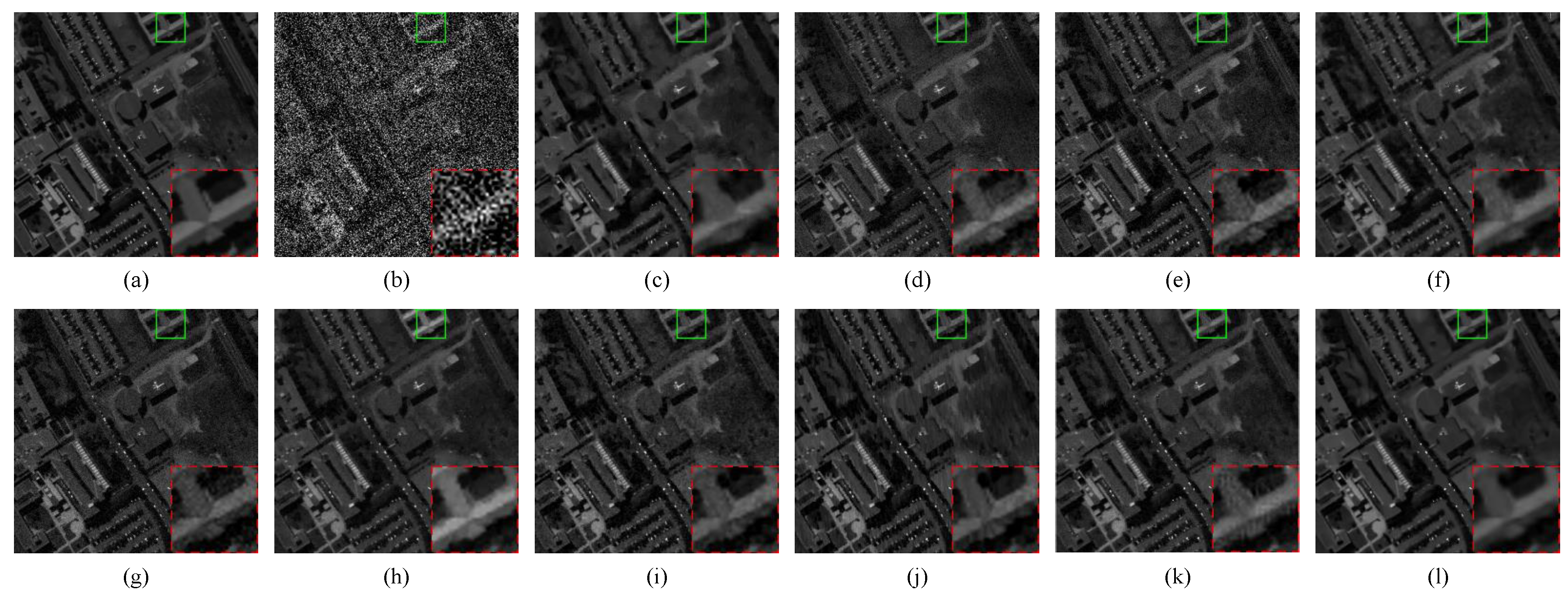
5.1.1. Visual Evaluation Results

For the visual performance of different methods, representative Case 1 and Case 6 are presented for evaluation. Figure 3 and Figure 4 illustrate the restoration results of WDC dataset. To further evaluate the visual results, zoom-in figures of specific area are enlarged in the bottom right corner.

As shown in Figure 3, the original band 1 of WDC is highly degraded by heavy Gaussian noise, ground information is completely unobservable. BM4D fails to remove noise and distorts the spatial domain of the image. LRMR, PCABM4D and TDL partially remove noise but are still unacceptable. FSSLRL, LLRSSTV, LRTDTV and LRTDGS are powerless in the front of heavy Gaussian noise. The non-local regularized method NLR-CPTD achieved fine removal of Gaussian noise, but there are still some gaps compared to SLRL4D. As the enlarged box shows, SLRL4D performs best in preserving details while the accurate restoration is realized successfully.

Same results are shown in Figure 4. Figure 4b indicates that band 110 of WDC in Case 6 is severely contaminated from mixed noises. Both BM4D, LRMR and PCABM4D failed their mission. TDL failed to completely remove the stripes. Four low-rank based methods, FSSLRL, LLRSSTV, LRTDTV and LRTDGS achieved fine removal of mixed noises, however, our proposed SLRL4D not only achieved the same outstanding mixed noises removal but also achieved the finest detail preservation according to the enlarged box. In addition, Figure 4k shows that the ability of NLR-CPTD in removing stripes partly decreases while heavy Gaussian noise exists.

Restoration results of all methods on PU dataset are shown in Figure 5 and Figure 6. Band 66 of the PU dataset is also degraded by heavy Gaussian noise. Among all methods, our SLRL4D method undoubtedly accomplished the best spatial information restoration as shown in the enlarged boxes of Figure 5. Severe mixed noises corrupted the band 82 of PU in Case 6, as shown in Figure 6b, and no progress was made by BM4D, LRMR, PCABM4D and TDL. Only FSSLRL, LLRSSTV and LRTDGS achieved the removal of mixed noises, but none of them ever transcended SLRL4D in spatial details preservation.

In summary, either with Gaussian noise or mixed noises, our SLRL4D method achieved the best results in visual performance for HSI restoration compared with all nine competitors. The superiority of low-rank learning and non-local filtering in the subspace of HSI is revealed.

5.1.2. Quantitative Evaluation Results

Five evaluation metrics with three positive metrics that is, the peak signal-to-noise ratio (PSNR), structure similarity (SSIM), feature similarity (FSIM) and two negative metrics, namely, erreur relative globale adimensionnellede synthese (ERGAS), and mean spectral angle (MSA) are invited to conduct a quantitative evaluation of our proposed method. The higher values of positive metrics indicate better restoration performance, as well as the lower values of negative metrics. Figure 7a–l shows the curves of the above three positive metrics comparison of all restoration methods on simulated WDC and PU datasets in Case 1 and Case 6. For Gaussian noise degraded Case 1 on WDC, SLRL4D achieved the highest PSNR, SSIM and FSIM in most of bands, and overwhelming dominance is achieved in more than half of all bands. Similar results occur in Case 6 on WDC which is heavily contaminated by mixed noises. SLRL4D still achieved optimal results in most of bands. Although the results in few bands are not optimal yet, the average results of all bands still exceed all competing methods. In Case 1 of PU dataset, our SLRL4D method purchased optimal PSNR and SSIM value effortlessly. Meanwhile, the same first-rank results happened in SSIM values of Case 6. As for rest metrics in the PU datasets, gratifying top-ranking results in all bands are also achieved. Meanwhile, the average optimum of all bands is also easily derived by SLRL4D.

Table 1. Quantitative Comparison under all six diverse case in simulated WDC and PU datasets.

Dataset	Case	Index	Noisy	PCABM4D [47]	TDL [58]	FSSLRL [49]	LLRSSTV [30]	LRTDTV [34]	LRTDGS [57]	NLR-CPTD [41]	SLRL4D
WDC	Case 1	PSNR	12.042	30.341	30.012	30.339	30.225	30.981	31.330	32.090	32.633
		SSIM	0.1330	0.8639	0.8647	0.8586	0.8529	0.8740	0.8871	0.9070	0.9208
		FSIM	0.4919	0.9328	0.9230	0.9330	0.9239	0.9299	0.9370	0.9475	0.9520
		ERGAS	60.8209	7.0790	7.3258	7.1147	7.3759	6.5940	6.3424	5.7895	5.4803
		MSA	0.8570	0.1307	0.1222	0.1302	0.1432	0.1050	0.1058	0.0976	0.0802
	Case 2	PSNR	14.129	31.534	31.422	31.611	31.539	32.150	32.410	33.396	33.439
		SSIM	0.1922	0.8966	0.8985	0.8985	0.8997	0.9008	0.9090	0.9288	0.9350
		FSIM	0.5539	0.9460	0.9416	0.9493	0.9419	0.9446	0.9485	0.9590	0.9607
		ERGAS	48.5655	6.1748	6.2320	6.1407	8.4325	5.7740	5.6087	5.0149	4.9961
		MSA	0.7572	0.1136	0.1059	0.1092	0.1607	0.0927	0.0925	0.0858	0.0742
	Case 3	PSNR	13.826	30.656	30.445	31.196	31.515	32.081	32.314	32.341	32.969
		SSIM	0.1831	0.8846	0.8818	0.8924	0.8989	0.8995	0.9087	0.9148	0.9224
		FSIM	0.5472	0.9428	0.9356	0.9469	0.9414	0.9441	0.9486	0.9540	0.9552
		ERGAS	50.5963	7.4086	7.5494	6.5403	9.6627	5.8170	5.6860	6.3406	5.4038
		MSA	0.7640	0.1486	0.1484	0.1260	0.1617	0.0926	0.0934	0.1280	0.0876
	Case 4	PSNR	13.948	30.427	31.408	31.503	31.809	31.893	32.248	32.144	33.312
		SSIM	0.1890	0.8816	0.8994	0.8957	0.8940	0.9005	0.9078	0.9143	0.9338
		FSIM	0.5486	0.9360	0.9425	0.9480	0.9431	0.9429	0.9478	0.9494	0.9599
		ERGAS	49.7693	7.6996	6.5065	6.2197	6.9987	6.0993	5.8574	6.3738	5.0699
		MSA	0.7651	0.1455	0.1143	0.1115	0.1381	0.0983	0.0955	0.1136	0.0751
	Case 5	PSNR	14.005	31.446	31.458	31.530	31.581	32.080	32.292	33.244	33.390
		SSIM	0.1892	0.8946	0.8970	0.8969	0.8928	0.8994	0.9102	0.9271	0.9284
		FSIM	0.5501	0.9451	0.9409	0.9481	0.9407	0.9438	0.9488	0.9577	0.9576
		ERGAS	49.5954	6.2429	6.2088	6.1925	8.1999	5.8178	5.7303	5.1017	5.0423
		MSA	0.7637	0.1146	0.1042	0.1099	0.1472	0.0935	0.0955	0.0869	0.0736
	Case 6	PSNR	13.790	30.141	30.639	31.110	31.788	32.047	32.217	31.748	32.919
		SSIM	0.1802	0.8765	0.8878	0.8925	0.8944	0.8995	0.9086	0.9059	0.9215
		FSIM	0.5458	0.9366	0.9388	0.9468	0.9438	0.9437	0.9481	0.9483	0.9553
		ERGAS	50.5140	8.4916	7.8616	6.6505	7.0572	5.8479	5.8564	7.2990	5.4843
		MSA	0.7654	0.1684	0.1575	0.1308	0.1380	0.0929	0.0963	0.1467	0.0903
PU	Case 1	PSNR	12.042	28.113	30.440	28.702	29.612	30.325	30.455	31.041	31.671
		SSIM	0.0892	0.7018	0.8408	0.7291	0.8194	0.7954	0.8217	0.8290	0.8717
		FSIM	0.4234	0.8831	0.9134	0.8970	0.9126	0.9016	0.9054	0.9206	0.9180
		ERGAS	61.3613	9.5350	7.3390	8.9760	8.2130	8.1152	7.6081	6.8476	6.3751
		MSA	0.9318	0.1885	0.1186	0.1764	0.1452	0.1702	0.1478	0.1385	0.0984
	Case 2	PSNR	14.097	29.555	31.599	30.144	30.529	31.744	31.549	32.495	32.643
		SSIM	0.1345	0.7656	0.8617	0.8035	0.8551	0.8435	0.8552	0.8672	0.8924
		FSIM	0.4847	0.9079	0.9316	0.9246	0.9277	0.9251	0.9221	0.9372	0.9321
		ERGAS	49.3741	8.1296	6.4632	7.6367	7.5414	6.9415	6.7190	5.9089	5.7106
		MSA	0.8319	0.1625	0.1159	0.1441	0.1336	0.1520	0.1349	0.1223	0.0916
	Case 3	PSNR	13.756	28.407	29.684	30.064	31.210	31.565	31.420	30.847	31.906
		SSIM	0.1253	0.7435	0.8123	0.7962	0.8282	0.8385	0.8518	0.8348	0.8799
		FSIM	0.4794	0.9014	0.9146	0.9221	0.9257	0.9240	0.9203	0.9240	0.9253
		ERGAS	51.0981	9.5420	8.5100	7.7057	6.8000	7.0056	6.8903	7.6459	6.2219
		MSA	0.8253	0.1930	0.1704	0.1432	0.1352	0.1517	0.1317	0.1646	0.1005
	Case 4	PSNR	14.056	28.232	30.186	30.278	31.354	31.750	31.386	30.635	32.506
		SSIM	0.1356	0.7452	0.8200	0.8049	0.8309	0.8442	0.8499	0.8449	0.8903
		FSIM	0.4841	0.8911	0.9183	0.9250	0.9255	0.9261	0.9195	0.9212	0.9316
		ERGAS	49.4070	10.1610	8.1262	7.5204	6.7023	6.8369	6.8518	8.2926	5.8021
		MSA	0.8261	0.2126	0.1613	0.1434	0.1359	0.1540	0.1357	0.1697	0.0945
	Case 5	PSNR	13.903	29.384	31.368	29.999	30.462	31.520	31.305	32.272	32.578
		SSIM	0.1295	0.7587	0.8538	0.7973	0.8523	0.8356	0.8470	0.8615	0.8912
		FSIM	0.4791	0.9054	0.9294	0.9228	0.9272	0.9216	0.9185	0.9345	0.9320
		ERGAS	50.4128	8.2778	6.6221	7.7509	7.5701	7.0474	6.8714	6.0468	5.7400
		MSA	0.8419	0.1648	0.1171	0.1465	0.1335	0.1552	0.1348	0.1245	0.0936
	Case 6	PSNR	13.469	27.448	28.899	29.932	31.067	31.334	31.238	29.485	31.811
		SSIM	0.1199	0.7197	0.7823	0.7892	0.8219	0.8289	0.8448	0.8109	0.8773
		FSIM	0.4705	0.8849	0.9087	0.9189	0.9226	0.9196	0.9171	0.9086	0.9238
		ERGAS	52.5291	11.0025	9.5224	7.8226	6.9016	7.1722	7.0374	9.2811	6.2780
		MSA	0.8339	0.2239	0.1910	0.1456	0.1371	0.1562	0.1369	0.1916	0.1025

demonstrates all the five quantitative evaluation metrics of seven competitive methods in WDC and PU datasets under all simulated cases. Due to the poor results of BM4D and LRMR, we have omitted them in this table. The optimal value of metrics among all competitive methods is highlighted in bold. As shown in Case 1 and Case 2, it is obvious that NLR-CPTD achieves second optimal PSNR, SSIM and FSIM values encountering heavy Gaussian noise.

The reason is that self-similarity of HSI is sufficiently utilized by the non-local regularization. However, our SLRL4D still performs better even NLR-CPTD reached competitive results. The superiority of non-local BM4D filtering is revealed compared with patch matching of NLR-CPTD. Meanwhile, as a BM4D filtering based method, PCABM4D achieved only average results. Both above phenomenas indicate that the combination of subspace low-rank learning and non-local BM4D filtering is sincerely powerful for getting rid of heavy Gaussian noise. Case 3–6 show that our proposed method almost achieved global optimal quantitative results in all cases in contrast with every competitor. Thus, the ability to remove mixed noises of SLRL4D is verified convincingly. NLR-CPTD performs delightful in heavy Gaussian noise, but its restoration results on mixed noises case is relativity inferior. LRTDTV and LRTDGS achieved pleasant consequences in mixed noises case, but compared with subspace-based SLRL4D, a conspicuous divergence still exists.

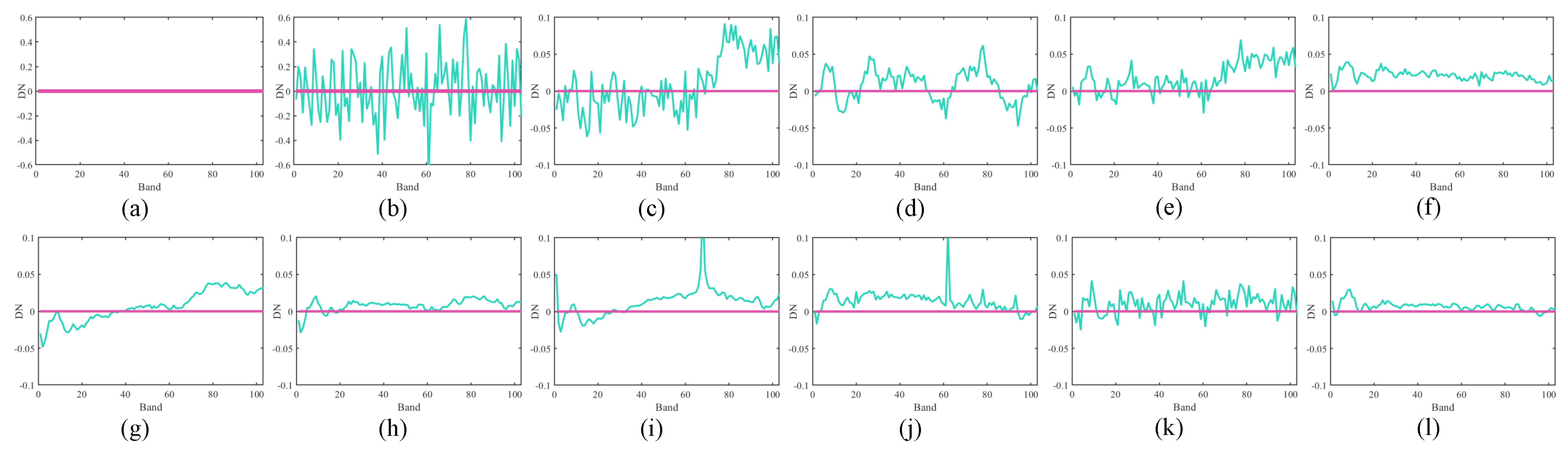
5.1.3. Qualitative Evaluation Results

For further illustrating the ability to preserve spectral signatures while restoring clean HSI of the SLRL4D method, the spectrum difference curves between original and restored HSI are presented in Figure 8, Figure 9, Figure 10 and Figure 11. As shown in Figure 8b, extensiveness fluctuations occurs at the spectrum of pixel (92, 218) in WDC under the contamination of heavy Gaussian noise. It is clear that our SLRL4D achieved most parallel signature of spectral after restoration. Figure 9 shows that in front of intricate mixed noises, BM4D, PCABM4D, TDL and NLR-CPTD disappointed the retrieval of spectral signatures.

This is unsurprising, particularly given their poor performance on mixed denoising. Combination methods of low-rank and other regularization terms that is, FSSLRL, LLRSSTV and LRTDTV achieved suboptimal spectral signatures preservation, but some middle-scale fluctuations still exist. Both LRTDGS and our SLRL4D makes splendid preservation of spectral signatures, but whether in visual comparison or quantitative analysis, far better results are always accomplished by SLRL4D.

Regarding to the PU dataset, approximate phenomena occurred as illustrated in Figure 10 and Figure 11. In either Case 1 or Case 6, the proposed method performs far better stability on spectrum difference images than any competitive method without even a hitch. Figure 10k–l indicates that while NLR-CPTD shows suboptimal ability on the removal of heavy Gaussian noise with the help of non-local regularization, its ability to maintain spectral correlation is far inferior to SLRL4D. As for mixed noises degraded Case 6, Figure 11 and Table 1 collectively indicate that our SLRL4D not only achieved better quantitative analyzed results than both LRTDTV and LRTDGS, the ability to restore spectral signatures of SLRL4D still exceeded them in the PU dataset. In conclusion, the proposed SLRL4D achieved not only optimal visual and quantitative performance but also transcendental preservation of spectral signatures.

5.1.4. Classification Evaluation Results

In this evaluation, we conducted the classification experiments on the restored Pavia University dataset to further verify the superiority of the proposed method. Representative case 1 and case 6 are employed.

Table 2. Classification accuracy for Case 1 and Case 6 of Pavia University dataset.

Case	Index	Noisy	PCABM4D [47]	TDL [58]	FSSLRL [49]	LLRSSTV [30]	LRTDTV [34]	LRTDGS [57]	NLR-CPTD [41]	SLRL4D
Case 1	OA	0.57732	0.70891	0.74824	0.60057	0.65361	0.71816	0.73532	0.76189	0.84743
	AA	0.52242	0.67714	0.68235	0.50377	0.55286	0.63976	0.66712	0.72033	0.80327
	Kappa	0.45628	0.63205	0.68247	0.46198	0.55072	0.64255	0.66595	0.70220	0.80847
Case 6	OA	0.59775	0.72702	0.73404	0.63980	0.66957	0.73811	0.75806	0.77881	0.86227
	AA	0.54232	0.69083	0.67431	0.54924	0.57729	0.65813	0.69144	0.72933	0.83022
	Kappa	0.48407	0.65680	0.66464	0.53553	0.57537	0.66784	0.69498	0.72158	0.82752

shows the classification results of restored HSI by every competitor and the proposed SLRL4D, respectively. The well-known support vector machine (SVM) [59,60,61] classier with RBF kernel is used for classification. Three indexes, that is, overall accuracy (OA), average accuracy (AA), and kappa statistic (Kappa), are employed for quantitative evaluation. Before classification, about 10% of samples are randomly selected from the labeled samples for training and the rest samples are for testing. Ten times of Monte Carlo runs are conducted and the averaged results are listed in Table 2. It leads us to conclude that restoration does improve the accuracy of classification, and better restoration delivers higher accuracy. The classification results once again verified that the proposed SLRL4D can accurately and effectively restore the HSI from mixed noise.

5.1.5. Comparison with Deep Learning Methods

In recent years, deep learning methods have earned a prestigious position that cannot be ignored in the field of computer vision [62,63,64,65,66]. Aiming to further verify the capacity of the proposed SLRL4D to remove heavy Gaussian noise, two state-of-the-art deep learning HSI denoising methods HSID-CNN [15] and HSI-SDeCNN [16] are employed for comparison. Similar to most deep learning methods, HSID-CNN and HSI-SDeCNN are mainly designed to remove Gaussian noise. Therefore, for a fair comparison, in the following experiments, we used the exact same WDC dataset and simulation manner of heavy Gaussian noise as in the article corresponding to HSI-SDeCNN [16], that is, the noise level ${\sigma }_n$ was set to [50, 75, 100]. The detailed quantitative evaluation results are shown in

Table 3. Comparison with Deep Learning Methods.

Noise Level	Index	BM4D [46]	HSID-CNN [15]	HSI-SDeCNN [16]	SLRL4D
${\sigma }_n=50$	PSNR	26.752	28.968	29.612	29.722
	SSIM	0.9208	0.9532	0.9608	0.9656
${\sigma }_n=75$	PSNR	24.261	26.753	27.351	28.045
	SSIM	0.8670	0.9273	0.9371	0.9489
${\sigma }_n=100$	PSNR	22.577	25.296	25.753	26.783
	SSIM	0.8119	0.9014	0.9121	0.9321

. Again, the optimal results are shown in bold font. It can be seen that the SLRL4D realizes better restoration than both latest deep learning methods from quantitative assessment.

5.2. Experimental Results on Real Datasets

5.2.1. Visual Evaluation Results

The aforementioned discussion demonstrated the outstanding ability in mixed denoising on the simulated datasets. However, noise degradation is far more intricate than simulation in real scenes.

Figure 12a shows the representative bands 103, 105, 144, 148 and 210 of the well-known real Urban dataset. In these five bands, the intensity of mixed noises is strengthened gradually. Except for band 103, which is slightly contaminated, the other four bands have been completely contaminated by a variety of heavy mixed noises, attempt to acquire any valuable information is absolutely impossible. For slightly contaminated band 103, PCABM4D, TDL, FSSLRL and LLRSSTV failed to remove the cross stripes, rest three comparison methods achieved the removal of stripes but spatial details contrast of some area are slightly enhanced as observed in the enlarged boxes. Both denoising and details preservation were achieved by our SLRL4D method. For band 105, as the noise density of mixed noises increases, PCABM4D, TDL and NLR-CPTD completely lose their power. Low-rank based methods FSSLRL and LRTDTV cannot deal with heavy stripes. LLRSSTV and LRTDGS achieved fine restoration results, but as shown in the enlarged boxes, distortion happened in the results, and, some areas became too bright in contrast with SLRL4D. For band 144, even LLRSSTV failed to remove the cross stripes. Similar to band 105, LRTDGS caused anamorphoses after restoration as shown in the enlarged box. The proposed SLRL4D successfully achieved delightful preservation of image details. Similar restoration results re-emerged on band 148. The difficulty of restoration was further increased, but SLRL4D still successfully accomplishes its mission without causing any abnormal brightness. As for band 210, SLRL4D also achieved optimal restoration results, the combination of subspace low-rank learning and subspace non-local filtering proved itself again.

5.2.2. Quantitative Evaluation Results

The horizontal mean profiles of bands 103, 105, 144, 148 and 210 on the HYDICE Urban dataset are shown in Figure 13. In each subfig, the horizontal axis represents the bands of urban dataset, and the vertical axis represents the digital number of horizontal mean profiles. As shown in Figure 13a, rapid fluctuations exist in the curve of the original bands due to the contamination of heavy mixed noises in all five bands. Particularly in the last three bands, severe mixed noises caused an abnormal jitter. As shown in Figure 13b–e and h, PCABM4D, TDL, FSSLRL, and LLRSSTV achieved inferior restoration performance. For non-local method NLR-CPTD, fine results are achieved only when the noises level are relativity mild. Figure 13f,g indicates that both LRTDTV and LRTDGS achieved relatively flat horizontal mean profiles curves. However, the blue box shows that compared with these two methods, our proposed method SLRL4D achieved flatter curves in all five bands, which indicates that the cross stripes and other diverse noises of Urban dataset have been eliminated more efficiently. In sum, competitive restoration results of our proposed SLRL4D were verified.

To further illustrate the efficiency of our proposed SLRL4D method in real scenarios, a blind non-reference assessment index named Q-metric was employed in our experiment to evaluate the restoration of spatial information.

Table 4. Blind Q-Metric comparison on HYDICE Urban and EO1-Hyperion datasets.

Dataset	Noisy	PCABM4D [47]	TDL [58]	FSSLRL [49]	LLRSSTV [30]	LRTDTV [34]	LRTDGS [57]	NLR-CPTD [41]	SLRL4D
Urban	0.06293	0.07881	0.06306	0.06217	0.06830	0.07408	0.07077	0.09202	0.09818
Hyperion	0.02432	0.03426	0.03198	0.03144	0.03198	0.03385	0.03716	0.03966	0.04459

lists the average Q values of all bands in both HYDICE Urban and EO-1 Hyperion datasets. A higher value of Q-metric yields a better restoration result. The optimal values are shown in bold. It can be seen that our proposed method SLRL4D acquires the best restoration indexes compared with all seven competitive methods.

The running time of an algorithm can effectively measure its efficiency.

Table 5. Running time comparison on HYDICE Urban and EO1-Hyperion datasets.

Dataset	PCABM4D [47]	TDL [58]	FSSLRL [49]	LLRSSTV [30]	LRTDTV [34]	LRTDGS [57]	NLR-CPTD [41]	SLRL4D
Urban	738.59	56.08	258.17	337.96	323.52	202.90	>1000	269.24
Hyperion	235.21	13.47	80.64	101.66	77.50	55.82	>1000	57.72

lists the running time comparison of all methods on two real datasets. Each method is run 10 times and averaged. In order to ensure the fairness of comparison, all methods are conducted in the same experimental environment, and the iteration times of those methods that require iterative solution is set to 50. As shown by the bold values, TDL achieved the fastest running speed of all methods, but its restoration results are also worse than most methods. The proposed SLRL4D achieved a competitive running time while ensuring the denoising performance.

6. Discussion

In our SLRL4D model, multiple parameters need to be discussed. With the help of BM4D filtering, no parameter of the non-local term requires to be tunning arduously, which makes our algorithm far more efficient and stable than exist non-local methods. Only subspace dimension p, penalty parameter $\mathsf{\mu }$, regularization parameters $\gamma$ and $\lambda$, which impact the nuclear norm and sparse norm respectively are left to be discussed. Obviously, less dependence on the parameters is achieved by our model in contrast with the congeneric methods.

6.1. The Impact of Parameters $\mu$, $\gamma$ and $\lambda$

Remarkable impacts were caused by the penalty parameter $\mathsf{\mu }$, as with the soft-thresholding parameter $\lambda$ and singular value thresholding parameters $\gamma$. More parameters bring more complex tunning, in order to make the method easier to use, we empirically set $\mathsf{\mu }=\left(10/\sqrt{max\left(d,l\right)}\right)\left(\sqrt{d}+\sqrt{l}\right)$ at first [49]. For regularization parameters $\gamma$ and $\lambda$, extensive experiments were conducted in the interval [0.1, 2] and [0.01, 0.1] to evaluate their sensitivity. As shown in Figure 14, mean PSNR, mean SSIM and ERGAS are employed to demonstrate the restoration performance of different parameter combinations on the mixed noises degraded Case 6 of the WDC dataset. It is easy to find that the proposed SLRL4D achieved delightful restoration results on a large scale of parameters, which indicates that our method does not require extremely specific parameter settings. Therefore, we recommend choosing $\gamma$ and $\lambda$ within the range of [0.1, 1] and [0.01, 0.05] respectively.

6.2. The Dimension of Subspace p

Theoretically, the number of endmembers in an HSI is the perfect candidate for the dimension of subspace p. The HySime signal identification algorithm is a highly effective tool to estimate p. For the simulated Case 6 under WDC dataset, HySime gives $p=3$ as the estimated dimension. However, as illustrated in Figure 15, both mean PSNR and MSA achieved the best results at $p=5$ instead of $p=3$. The primary cause of this phenomenon is that HySime only delivers precise estimation for Gaussian degraded signals. Therefore, for the case of mixed noises, we recommend choosing subspace dimension p within the range of [3, 8] according to the specific degradation status itself.

All our experiments select parameters in the above ranges, for instance, the parameters used on simulated case 1–6 of the WDC dataset are listed in

Table 6. Parameters used on simulated case 1–6 of the WDC dataset.

	Case	Case 1	Case 2	Case 3	Case 4	Case 5	Case 6
Parameter
$\lambda$		1	1	0.2	0.4	0.4	0.2
$\gamma$		0.02	0.02	0.02	0.02	0.02	0.02
p		4	4	5	4	5	4

.

6.3. Convergence Analysis

Figure 16 shows the rising tendency of the PSNR and SSIM under simulated Case 6 of WDC dataset along with the increase of iterations, both the PSNR and SSIM achieved convergence after rapid growth in the initial few iterations, hence the rapid convergence of the proposed SLRL4D is verified.

7. Conclusions and Future Work

Focusing on the mixed noises degeneration problem of HSI, in this paper, a joint method of subspace low-rank learning and nonlocal 4-d transform filtering is presented for HSI restoration. In summary, both spatial-spectral correlations of HSI are explored comprehensively through joint low-rank regularization and non-local 4-d filtering in the subspace decomposition framework. In this manner, the low-rank property in the spectral domain and the non-local self-similarity of the spatial domain are exploited simultaneously. In contrast with utilizing prior in original space, our proposed subspace-based method not only obtained better restoration results but also cost lower computational resource. The carefully designed restoration model is efficiently solved by the convex optimization algorithm. Extensive experimental evaluations on multiple simulated and real datasets validate that our proposed HSI restoration method is both effective and efficient. For future work, the tensor representation based subspace low-rank learning methods will be considered to further improve the performance, and more precise non-local self-similarity regularization of spatial domain of HSI will be explored. Meanwhile, using low-rankness for image compression is also worth further study.

References

1. Bioucas-Dias, J.M.; Plaza, A.; Camps-Valls, G.; Scheunders, P.; Nasrabadi, N.; Chanussot, J. Hyperspectral remote sensing data analysis and future challenges. IEEE Geosci. Remote Sens. Mag. 2013, 1, 6–36. [Google Scholar] [CrossRef] [Green Version]
2. Imani, M.; Ghassemian, H. An overview on spectral and spatial information fusion for hyperspectral image classification: Current trends and challenges. Inf. Fusion 2020, 59, 59–83. [Google Scholar] [CrossRef]
3. Lu, X.; Dong, L.; Yuan, Y. Subspace clustering constrained sparse NMF for hyperspectral unmixing. IEEE Trans. Geosci. Remote Sens. 2020, 58, 3007–3019. [Google Scholar] [CrossRef]
4. Moeini Rad, A.; Abkar, A.A.; Mojaradi, B. Supervised distance-based feature selection for hyperspectral target detection. Remote Sens. 2019, 11, 2049. [Google Scholar] [CrossRef] [Green Version]
5. Sun, L.; Ma, C.; Chen, Y.; Zheng, Y.; Shim, H.J.; Wu, Z.; Jeon, B. Low rank component Induced spatial-spectral kernel method for hyperspectral image classification. IEEE Trans. Circuits Syst. Video Technol. 2020, 1. [Google Scholar] [CrossRef]
6. Chen, Y.; Li, J.; Zhou, Y. Hyperspectral image denoising by total variation-regularized bilinear factorization. Signal Process. 2020, 174, 107645. [Google Scholar] [CrossRef]
7. Othman, H.; Qian, S.E. Noise reduction of hyperspectral imagery using hybrid spatial-spectral derivative-domain wavelet shrinkage. IEEE Trans. Geosci. Remote Sens. 2006, 44, 397–408. [Google Scholar] [CrossRef]
8. Chen, G.; Qian, S.E. Denoising of hyperspectral imagery using principal component analysis and wavelet shrinkage. IEEE Trans. Geosci. Remote Sens. 2010, 49, 973–980. [Google Scholar] [CrossRef]
9. Zhang, X.; Peng, F.; Long, M. Robust coverless image steganography based on DCT and LDA topic classification. IEEE Trans. Multimed. 2018, 20, 3223–3238. [Google Scholar] [CrossRef]
10. Buades, A.; Coll, B.; Morel, J.M. A non-local algorithm for image denoising. In Proceedings of the 2005 IEEE Computer Society Conference on Computer Vision and Pattern Recognition (CVPR’05), San Diego, CA, USA, 20–25 June 2005; Volume 2, pp. 60–65. [Google Scholar]
11. Qian, Y.; Ye, M. Hyperspectral imagery restoration using nonlocal spectral-spatial structured sparse representation with noise estimation. IEEE J. Sel. Top. Appl. Earth Obs. Remote Sens. 2012, 6, 499–515. [Google Scholar] [CrossRef]
12. Song, Y.; Cao, W.; Shen, Y.; Yang, G. Compressed sensing image reconstruction using intra prediction. Neurocomputing 2015, 151, 1171–1179. [Google Scholar] [CrossRef]
13. Song, Y.; Yang, G.; Xie, H.; Zhang, D.; Sun, X. Residual domain dictionary learning for compressed sensing video recovery. Multimed. Tools Appl. 2017, 76, 10083–10096. [Google Scholar] [CrossRef]
14. Shen, Y.; Li, J.; Zhu, Z.; Cao, W.; Song, Y. Image reconstruction algorithm from compressed sensing measurements by dictionary learning. Neurocomputing 2015, 151, 1153–1162. [Google Scholar] [CrossRef]
15. Yuan, Q.; Zhang, Q.; Li, J.; Shen, H.; Zhang, L. Hyperspectral image denoising employing a spatial–spectral deep residual convolutional neural network. IEEE Trans. Geosci. Remote Sens. 2019, 57, 1205–1218. [Google Scholar] [CrossRef] [Green Version]
16. Maffei, A.; Haut, J.M.; Paoletti, M.E.; Plaza, J.; Bruzzone, L.; Plaza, A. A single model CNN for hyperspectral image denoising. IEEE Trans. Geosci. Remote Sens. 2020, 58, 2516–2529. [Google Scholar] [CrossRef]
17. Long, M.; Zeng, Y. Detecting iris liveness with batch normalized convolutional neural network. Comput. Mater. Contin. 2019, 58, 493–504. [Google Scholar] [CrossRef]
18. Zhang, J.; Jin, X.; Sun, J.; Wang, J.; Sangaiah, A.K. Spatial and semantic convolutional features for robust visual object tracking. Multimed. Tools Appl. 2020, 79, 15095–15115. [Google Scholar] [CrossRef]
19. Zeng, D.; Dai, Y.; Li, F.; Wang, J.; Sangaiah, A.K. Aspect based sentiment analysis by a linguistically regularized CNN with gated mechanism. J. Intell. Fuzzy Syst. 2019, 36, 3971–3980. [Google Scholar] [CrossRef]
20. Candès, E.J.; Li, X.; Ma, Y.; Wright, J. Robust principal component analysis? J. ACM (JACM) 2011, 58, 1–37. [Google Scholar] [CrossRef]
21. Zhang, H.; He, W.; Zhang, L.; Shen, H.; Yuan, Q. Hyperspectral image restoration using low-rank matrix recovery. IEEE Trans. Geosci. Remote Sens. 2013, 52, 4729–4743. [Google Scholar] [CrossRef]
22. Wang, Q.; He, X.; Li, X. Locality and structure regularized low rank representation for hyperspectral image classification. IEEE Trans. Geosci. Remote Sens. 2018, 57, 911–923. [Google Scholar] [CrossRef] [Green Version]
23. Zhao, Y.Q.; Yang, J. Hyperspectral image denoising via sparse representation and low-rank constraint. IEEE Trans. Geosci. Remote Sens. 2014, 53, 296–308. [Google Scholar] [CrossRef]
24. Chen, Y.; Huang, T.Z.; Zhao, X.L.; Deng, L.J. Hyperspectral image restoration using framelet-regularized low-rank nonnegative matrix factorization. Appl. Math. Model. 2018, 63, 128–147. [Google Scholar] [CrossRef]
25. Rudin, L.I.; Osher, S.; Fatemi, E. Nonlinear total variation based noise removal algorithms. Phys. D: Nonlinear Phenom. 1992, 60, 259–268. [Google Scholar] [CrossRef]
26. Aggarwal, H.K.; Majumdar, A. Hyperspectral image denoising using spatio-spectral total variation. IEEE Geosci. Remote Sens. Lett. 2016, 13, 442–446. [Google Scholar] [CrossRef]
27. Wu, Z.; Wang, Q.; Wu, Z.; Shen, Y. Total variation-regularized weighted nuclear norm minimization for hyperspectral image mixed denoising. J. Electron. Imaging 2016, 25, 013037. [Google Scholar] [CrossRef]
28. Wang, Q.; Wu, Z.; Jin, J.; Wang, T.; Shen, Y. Low rank constraint and spatial spectral total variation for hyperspectral image mixed denoising. Signal Process. 2018, 142, 11–26. [Google Scholar] [CrossRef]
29. He, W.; Zhang, H.; Zhang, L.; Shen, H. Total-variation-regularized low-rank matrix factorization for hyperspectral image restoration. IEEE Trans. Geosci. Remote Sens. 2015, 54, 178–188. [Google Scholar] [CrossRef]
30. He, W.; Zhang, H.; Shen, H.; Zhang, L. Hyperspectral image denoising using local low-rank matrix recovery and global spatial–spectral total variation. IEEE J. Sel. Top. Appl. Earth Obs. Remote Sens. 2018, 11, 713–729. [Google Scholar] [CrossRef]
31. Fang, Y.; Li, H.; Ma, Y.; Liang, K.; Hu, Y.; Zhang, S.; Wang, H. Dimensionality reduction of hyperspectral images based on robust spatial information using locally linear embedding. IEEE Geosci. Remote Sens. Lett. 2014, 11, 1712–1716. [Google Scholar] [CrossRef]
32. Xue, J.; Zhao, Y.; Liao, W.; Chan, J.C.W. Nonconvex tensor rank minimization and its applications to tensor recovery. Inf. Sci. 2019, 503, 109–128. [Google Scholar] [CrossRef]
33. Fan, H.; Chen, Y.; Guo, Y.; Zhang, H.; Kuang, G. Hyperspectral image restoration using low-rank tensor recovery. IEEE J. Sel. Top. Appl. Earth Obs. Remote Sens. 2017, 10, 4589–4604. [Google Scholar] [CrossRef]
34. Wang, Y.; Peng, J.; Zhao, Q.; Leung, Y.; Zhao, X.L.; Meng, D. Hyperspectral image restoration via total variation regularized low-rank tensor decomposition. IEEE J. Sel. Top. Appl. Earth Obs. Remote Sens. 2018, 11, 1227–1243. [Google Scholar] [CrossRef] [Green Version]
35. Yang, J.H.; Zhao, X.L.; Ma, T.H.; Chen, Y.; Huang, T.Z.; Ding, M. Remote sensing images destriping using unidirectional hybrid total variation and nonconvex low-rank regularization. J. Comput. Appl. Math. 2020, 363, 124–144. [Google Scholar] [CrossRef]
36. Mairal, J.; Bach, F.; Ponce, J.; Sapiro, G.; Zisserman, A. Non-local sparse models for image restoration. In Proceedings of the 2009 IEEE 12th International Conference on Computer Vision, Kyoto, Japan, 29 September–2 October 2009; pp. 2272–2279. [Google Scholar]
37. Katkovnik, V.; Foi, A.; Egiazarian, K.; Astola, J. From local kernel to nonlocal multiple-model image denoising. Int. J. Comput. Vis. 2010, 86, 1. [Google Scholar] [CrossRef] [Green Version]
38. Zhu, R.; Dong, M.; Xue, J.H. Spectral nonlocal restoration of hyperspectral images with low-rank property. IEEE J. Sel. Top. Appl. Earth Obs. Remote Sens. 2014, 8, 3062–3067. [Google Scholar]
39. Bai, X.; Xu, F.; Zhou, L.; Xing, Y.; Bai, L.; Zhou, J. Nonlocal similarity based nonnegative tucker decomposition for hyperspectral image denoising. IEEE J. Sel. Top. Appl. Earth Obs. Remote Sens. 2018, 11, 701–712. [Google Scholar] [CrossRef] [Green Version]
40. Xue, J.; Zhao, Y.; Liao, W.; Kong, S.G. Joint spatial and spectral low-rank regularization for hyperspectral image denoising. IEEE Trans. Geosci. Remote Sens. 2017, 56, 1940–1958. [Google Scholar] [CrossRef]
41. Xue, J.; Zhao, Y.; Liao, W.; Chan, J.C.W. Nonlocal low-rank regularized tensor decomposition for hyperspectral image denoising. IEEE Trans. Geosci. Remote Sens. 2019, 57, 5174–5189. [Google Scholar] [CrossRef]
42. Xie, Q.; Zhao, Q.; Meng, D.; Xu, Z.; Gu, S.; Zuo, W.; Zhang, L. Multispectral images denoising by intrinsic tensor sparsity regularization. In Proceedings of the IEEE Conference on Computer Vision and Pattern Recognition, Las Vegas, NV, USA, 27–30 June 2016; pp. 1692–1700. [Google Scholar]
43. Huang, Z.; Li, S.; Fang, L.; Li, H.; Benediktsson, J.A. Hyperspectral image denoising with group sparse and low-rank tensor decomposition. IEEE Access 2017, 6, 1380–1390. [Google Scholar] [CrossRef]
44. Zhang, H.; Liu, L.; He, W.; Zhang, L. Hyperspectral image denoising with total variation regularization and nonlocal low-rank tensor decomposition. IEEE Trans. Geosci. Remote Sens. 2019, 58, 3071–3084. [Google Scholar] [CrossRef]
45. Chen, Y.; He, W.; Yokoya, N.; Huang, T.Z.; Zhao, X.L. Nonlocal tensor-ring decomposition for hyperspectral image denoising. IEEE Trans. Geosci. Remote Sens. 2019, 58, 1348–1362. [Google Scholar] [CrossRef]
46. Maggioni, M.; Katkovnik, V.; Egiazarian, K.; Foi, A. Nonlocal transform-domain filter for volumetric data denoising and reconstruction. IEEE Trans. Image Process. 2012, 22, 119–133. [Google Scholar] [CrossRef] [PubMed]
47. Chen, G.; Bui, T.D.; Quach, K.G.; Qian, S.E. Denoising hyperspectral imagery using principal component analysis and block-matching 4D filtering. Can. J. Remote Sens. 2014, 40, 60–66. [Google Scholar] [CrossRef]
48. Sun, L.; Jeon, B. A novel subspace spatial-spectral low rank learning method for hyperspectral denoising. In Proceedings of the 2017 IEEE Visual Communications and Image Processing (VCIP), St. Petersburg, FL, USA, 10–13 December 2017; pp. 1–4. [Google Scholar]
49. Sun, L.; Jeon, B.; Soomro, B.N.; Zheng, Y.; Wu, Z.; Xiao, L. Fast superpixel based subspace low rank learning method for hyperspectral denoising. IEEE Access 2018, 6, 12031–12043. [Google Scholar] [CrossRef]
50. Zhuang, L.; Bioucas-Dias, J.M. Fast hyperspectral image denoising and inpainting based on low-rank and sparse representations. IEEE J. Sel. Top. Appl. Earth Obs. Remote Sens. 2018, 11, 730–742. [Google Scholar] [CrossRef]
51. He, W.; Yao, Q.; Li, C.; Yokoya, N.; Zhao, Q. Non-local meets global: An integrated paradigm for hyperspectral denoising. In Proceedings of the 2019 IEEE/CVF Conference on Computer Vision and Pattern Recognition (CVPR), Long Beach, CA, USA, 15–20 June 2019; pp. 6861–6870. [Google Scholar]
52. Zhuang, L.; Ng, M.K. Hyperspectral mixed noise temoval by l_1-norm-based subspace representation. IEEE J. Sel. Top. Appl. Earth Obs. Remote Sens. 2020, 13, 1143–1157. [Google Scholar] [CrossRef]
53. Huang, H.; Shi, G.; He, H.; Duan, Y.; Luo, F. Dimensionality reduction of hyperspectral imagery based on spatial–spectral manifold learning. IEEE Trans. Cybern. 2019, 50, 2604–2616. [Google Scholar] [CrossRef] [Green Version]
54. Boyd, S.; Parikh, N.; Chu, E.; Peleato, B.; Eckstein, J. Distributed optimization and statistical learning via the alternating direction method of multipliers. Found. Trends Mach. Learn. 2011, 3, 1–122. [Google Scholar] [CrossRef]
55. Bioucas-Dias, J.M.; Nascimento, J.M. Hyperspectral subspace identification. IEEE Trans. Geosci. Remote Sens. 2008, 46, 2435–2445. [Google Scholar] [CrossRef] [Green Version]
56. Sun, L.; Wu, F.; Zhan, T.; Liu, W.; Wang, J.; Jeon, B. Weighted nonlocal low-rank tensor decomposition method for sparse unmixing of hyperspectral images. IEEE J. Sel. Top. Appl. Earth Obs. Remote Sens. 2020, 13, 1174–1188. [Google Scholar] [CrossRef]
57. Chen, Y.; He, W.; Yokoya, N.; Huang, T.Z. Hyperspectral image restoration using weighted group sparsity-regularized low-rank tensor decomposition. IEEE Trans. Cybern. 2020, 50, 3556–3570. [Google Scholar] [CrossRef] [PubMed]
58. Peng, Y.; Meng, D.; Xu, Z.; Gao, C.; Yang, Y.; Zhang, B. Decomposable nonlocal tensor dictionary learning for multispectral image denoising. In Proceedings of the IEEE Conference on Computer Vision and Pattern Recognition, Columbus, OH, USA, 23–28 June 2014; pp. 2949–2956. [Google Scholar]
59. Kuang, F.; Zhang, S.; Jin, Z.; Xu, W. A novel SVM by combining kernel principal component analysis and improved chaotic particle swarm optimization for intrusion detection. Soft Comput. 2015, 19, 1187–1199. [Google Scholar] [CrossRef]
60. Chen, Y.; Xiong, J.; Xu, W.; Zuo, J. A novel online incremental and decremental learning algorithm based on variable support vector machine. Clust. Comput. 2019, 22, 7435–7445. [Google Scholar] [CrossRef]
61. Chen, Y.; Xu, W.; Zuo, J.; Yang, K. The fire recognition algorithm using dynamic feature fusion and IV-SVM classifier. Clust. Comput. 2019, 22, 7665–7675. [Google Scholar] [CrossRef]
62. Zeng, D.; Dai, Y.; Li, F.; Sherratt, R.S.; Wang, J. Adversarial learning for distant supervised relation extraction. Comput. Mater. Contin. 2018, 55, 121–136. [Google Scholar]
63. Meng, R.; Rice, S.G.; Wang, J.; Sun, X. A fusion steganographic algorithm based on faster R-CNN. Comput. Mater. Contin. 2018, 55, 1–16. [Google Scholar]
64. Zhou, S.; Ke, M.; Luo, P. Multi-camera transfer GAN for person re-identification. J. Vis. Commun. Image Represent. 2019, 59, 393–400. [Google Scholar] [CrossRef]
65. He, S.; Li, Z.; Tang, Y.; Liao, Z.; Li, F.; Lim, S.J. Parameters compressing in deep learning. Comput. Mater. Contin. 2020, 62, 321–336. [Google Scholar] [CrossRef]
66. Gui, Y.; Zeng, G. Joint learning of visual and spatial features for edit propagation from a single image. Vis. Comput. 2020, 36, 469–482. [Google Scholar] [CrossRef]
Figure 1. Singular values comparison of the original Urban hyperspectral image (HSI) and the corresponding subspace.
Remotesensing 12 02979 g001
Figure 2. Flowchart of the proposed subspace low-rank learning and non-local 4-d transform filtering (SLRL4D) method.
Remotesensing 12 02979 g002
Figure 3. Visual comparison on band 1 of Washington DC Mall (WDC) dataset under simulated Case 1. (a) Original. (b) Contaminated. (c)BM4D. (d) LRMR. (e) PCABM4D. (f) TDL. (g) FSSLRL. (h) LLRSSTV. (i) LRTDTV. (j) LRTDGS. (k) NLR-CPTD. (l) SLRL4D.
Remotesensing 12 02979 g003
Figure 4. Visual comparison on band 110 of WDC dataset under simulated Case 6. (a) Original. (b) Contaminated. (c) BM4D. (d) LRMR. (e) PCABM4D. (f) TDL. (g) FSSLRL. (h) LLRSSTV. (i) LRTDTV. (j) LRTDGS. (k) NLR-CPTD. (l) SLRL4D.
Remotesensing 12 02979 g004
Figure 5. Visual comparison on band 66 of PU dataset under simulated Case 1. (a) Original. (b) Contaminated. (c) BM4D. (d) LRMR. (e) PCABM4D. (f) TDL. (g) FSSLRL. (h) LLRSSTV. (i) LRTDTV. (j) LRTDGS. (k) NLR-CPTD. (l) SLRL4D.
Remotesensing 12 02979 g005
Figure 6. Visual comparison on band 82 of PU dataset under simulated Case 6. (a) Original. (b) Contaminated. (c) BM4D. (d) LRMR. (e) PCABM4D. (f) TDL. (g) FSSLRL. (h) LLRSSTV. (i) LRTDTV. (j) LRTDGS. (k) NLR-CPTD. (l) SLRL4D.
Remotesensing 12 02979 g006
Figure 7. Peak signal-to-noise ratio (PSNR), structure similarity (SSIM), feature similarity (FSIM) comparison of all restoration methods under simulation Case 1 and Case 6. (ac) Case 1 of WDC dataset. (df) Case 6 of WDC dataset. (gi) Case 1 of Pavia University (PU) dataset. (jl) Case 6 of PU dataset.
Remotesensing 12 02979 g007
Figure 8. Spectrum difference comparison in pixel (92, 218) of WDC under Case 1. (a) Original, (b) Contaminated, (c) BM4D, (d) LRMR, (e) PCABM4D, (f) TDL, (g) FSSLRL, (h) LLRSSTV, (i) LRTDTV, (j) LRTDGS, (k) NLR-CPTD, (l) SLRL4D.
Remotesensing 12 02979 g008
Figure 9. Spectrum difference comparison in pixel (53, 129) of WDC under Case 6. (a) Original, (b) Contaminated, (c) BM4D, (d) LRMR, (e) PCABM4D, (f) TDL, (g) FSSLRL, (h) LLRSSTV, (i) LRTDTV, (j) LRTDGS, (k) NLR-CPTD, (l) SLRL4D.
Remotesensing 12 02979 g009
Figure 10. Spectrum difference comparison in pixel (140, 105) of PU under Case 1. (a) Original, (b) Contaminated, (c) BM4D, (d) LRMR, (e) PCABM4D, (f) TDL, (g) FSSLRL, (h) LLRSSTV, (i) LRTDTV, (j) LRTDGS, (k) NLR-CPTD, (l) SLRL4D.
Remotesensing 12 02979 g010
Figure 11. Spectrum difference comparison in pixel (72, 150) of PU under Case 6. (a) Original, (b) Contaminated, (c) BM4D, (d) LRMR, (e) PCABM4D, (f) TDL, (g) FSSLRL, (h) LLRSSTV, (i) LRTDTV, (j) LRTDGS, (k) NLR-CPTD, (l) SLRL4D.
Remotesensing 12 02979 g011
Figure 12. Visual comparison of all restoration methods on bands 103, 105, 144, 148, 210 of HYDICE Urban dataset. (a) Original, (b) PCABM4D, (c) TDL, (d) FSSLRL, (e) LLRSSTV, (f) LRTDTV, (g) LRTDGS, (h) NLR-CPTD, (i) SLRL4D.
Remotesensing 12 02979 g012
Figure 13. Horizontal mean profiles comparison of all methods on bands 103, 105, 144, 148, 210 of HYDICE Urban dataset. (a) Original, (b) PCABM4D, (c) TDL, (d) FSSLRL, (e) LLRSSTV, (f) LRTDTV, (g) LRTDGS, (h) NLR-CPTD, (i) SLRL4D.
Remotesensing 12 02979 g013
Figure 14. Sensitivity analysis of parameters λ and γ by employing PSNR, SSIM and erreur relative globale adimensionnellede synthese (ERGAS) under Case 6 of simulated WDC dataset. (a) PSNR, (b) SSIM, (c) ERGAS.
Remotesensing 12 02979 g014
Figure 15. Sensitivity analysis of subspace dimension p by employing PSNR and mean spectral angle (MSA) under Case 6 of simulated WDC dataset. (a) PSNR, (b) MSA.
Remotesensing 12 02979 g015
Figure 16. Convergence analysis of SLRL4D by employing PSNR and SSIM under Case 6 of simulated WDC dataset. (a) PSNR, (b) SSIM.
Remotesensing 12 02979 g016