Spatial Configuration and Extent Explains the Urban Heat Mitigation Potential due to Green Spaces: Analysis over Addis Ababa, Ethiopia

Abstract

Urban green space (UGS) is considered a mitigative intervention for urban heat. While increasing the UGS coverage is expected to reduce the urban heat, studies on the effects of UGS configuration have produced inconsistent results. To investigate this inconsistency further, this study conducted a multi-spatial and multi-temporal resolution analysis in the Addis Ababa city metropolitan area for assessing the relationship between UGS patterns and land surface temperature (LST). Landsat images were used to generate land cover and LST maps. Regression models were developed to investigate whether controlling for the proportion of the green area (PGS), fragmentation, shape, complexity, and proximity distance can affect surface temperature. Results indicated that the UGS patches with aggregated, regular and simple shapes and connectivity throughout the urban landscape were more effective in decreasing the LST as compared to the fragmented and complicated spatial patterns. This finding highlighted that in addition to increasing the amount of UGS, optimizing the spatial structure of UGS, could be an effective and useful action to mitigate the urban heat island (UHI) impacts. Changing the spatial size had a significant influence on the interconnection between LST and UGS patterns as well. It also noted that the spatial arrangement of UGS was more sensitive to spatial scales than that of its composition. The relationship between the spatial configuration of UGS and LST could be changed when applying different statistical methods. This result underlined the importance of controlling the effects of the share of green spaces when calculating the impacts of the spatial configuration of UGS on LST. Furthermore, the study highlighted that applying different statistical approaches, spatial scale, and coverage of UGS can help determine the effectiveness of the association between LST and UGS patterns. These outcomes provided new insights regarding the inconsistent findings from earlier studies, which might be a result of the different approaches considered. Indeed, these findings are expected to be of help more broadly for city planning and urban heat mitigation.

1. Introduction

Over half the global population dwells in cities [1]. Urbanization is typically associated with providing better socio-economic conditions. On the other end, urbanization has also been associated with environmental and ecological stresses [2,3,4]. One of the widely recorded and evident impacts associated with urbanization is the increased temperature over the cities relative to the adjacent rural areas, or the urban heat island (UHI) [5,6]. Relative to the rural regions, urban areas have distinct morphology, geometry, and infrastructure that contributes to the UHI. Changes in land use and land cover result in an abundance of built impervious surfaces and depletion of green vegetation covers, causing alterations in the surface energy fluxes [6,7,8,9], distribution and composition of biodiversity [10,11], increasing anthropogenic heat releases [12], and human health [13,14]. As a result, how to understand and mitigate these adverse impacts has become a key study topic in urban ecology, geography, and climatology [15,16,17,18].

Spatial patterns and intensity of UHI are determined by the size of the population and impervious surface [4,19,20,21], land cover types [15,22,23,24,25], spatial patterns of green space [16,26,27,28], urban spatial structure [2,4,29,30,31,32], socioeconomic activities [33,34], and climate conditions [15,35,36,37]. Broadly, two major categories of UHI have been identified depending upon the substrate of their influences: air (atmospheric) and surface. The atmospheric UHI and the surface temperature are highly correlated to health, though the air UHI impact is reflected to be intimately connected to human health [38]. The in-situ measurement techniques used for atmospheric UHI monitoring [37,38,39,40], have the advantages of better temporal resolution but lack spatial resolution. Whereas the surface land surface temperature (LST) is typically mapped using satellite data from thermal sensors [41,42,43]. Thermal remote sensing makes use of non-contact instruments to sense thermal radiations and estimate surface or skin temperatures. Nevertheless, thermal remote sensing has its limitation of poor temporal coverage, coarse spatial resolution, and the requirement for clear weather conditions.

Many studies have estimated LST from medium-resolution remotely sensed satellite data (e.g., Landsat) for long-term temperature observations from the early 1980s. For instance, the significant cooling effects of urban green space (UGS) spatial patterns on the urban heat have been widely demonstrated by previous researches [22,24,35,44,45,46,47]. Spatial pattern encompasses composition (the amounts and diversities of land cover types), as well as configuration (their distribution and structure). Urban landscapes are composed of several diverse land cover varieties, while built-up and vegetated cover are two essential features in the UHI formation [48]. Accordingly, it is known that increasing the amount of green space can significantly reduce the ambient air and land surface temperature [16,43,44]. This correlation has been reported consistently and follows the first principle surface radiative flux balance at the surface. Several studies also confirmed that the arrangement (configuration) of green space had considerable impacts on land surface temperature [2,26,31,49,50]. However, these studies produced contradictory findings. Green space with higher patch density, for instance, decreased LST in research carried out in the Phoenix metropolitan area, USA [51], Lagos, Nigeria [39], Shanghai, China [16], regions across Illinois-Indiana-Ohio, USA [19], and Berlin, Germany [52]. On the other hand, green space density was associated with increased LST in Jakarta, Indonesia [53], and Nairobi, Kenya [54]. In addition, the edge density of green space had negatively correlated to LST with several cities [42,43,49,51], and contrarily, it was positively correlated with others [45,55]. These inconsistencies are likely due to the following reasons. (i) using a single snapshot data for individual cities with multiple approaches [39,45]; (ii) implementing different images of data with varied spatial resolutions [21,42,55,56]; (iii) applying a different statistical analysis [2,16,45,53]; and (iv) using a different spatial scale (analytical unit) such as circular plots [26,51,57,58], sub-zones (16,30,43,45), pixels or grids [59], or city blocks [52].

Although the above-stated factors could be reasons for the inconsistency findings in the prior studies, such contradictory results could restrict the application of findings for planning and managing the urban green space. Hence, further investigation is warranted. Moreover, urban regions are complex systems [20,60]. The phenomenon associated with urban landscape characteristics is scale-dependent. When the scale of observation is altered, the correlation between pattern and process phenomenon will change [16,42,45]. Hence, recognizing how the urban green space pattern influences the surface energy balance and the variability of LST needs, the analytical size exemplifies the characteristic spatial extent of LST and green space interaction. As noted in previous studies, there are two broad methods to accomplish this aim: (1) using a single city study to explore temporal dynamics [43,57], and (2) a comparative study of multiple cities applying similar approaches [45,53]. The present study adopts the first approach, to address the following questions: (i) does the spatial pattern of UGS affect temperatures differently in the city with changes over time? and (ii) do different statistical approaches or analytical units result in different effects of the spatial configuration of UGS on LST?

To answer these questions, the study analyzed the relationships between the LST and spatial configuration of UGS by using different statistical methods, and varied spatial configuration across different periods in the metropolitan area of Addis Ababa, Ethiopia. Landsat images were used to produce the land cover and LST maps. As cities have mostly limited space for greening [16,29,43], this study provides empirical results that can improve the understanding of the seemingly contradictory impacts of the spatial configuration of UGS patterns on LST noted in earlier studies. Such empirical results can potentially help planners and managers in regulating the spatial arrangement of urban green space to mitigate UHI. Furthermore, the adopted integrated approaches, multiple statistical, and landscape metrics analysis at varied analytical units, provide comprehensive and detailed information for environmental planning issues.

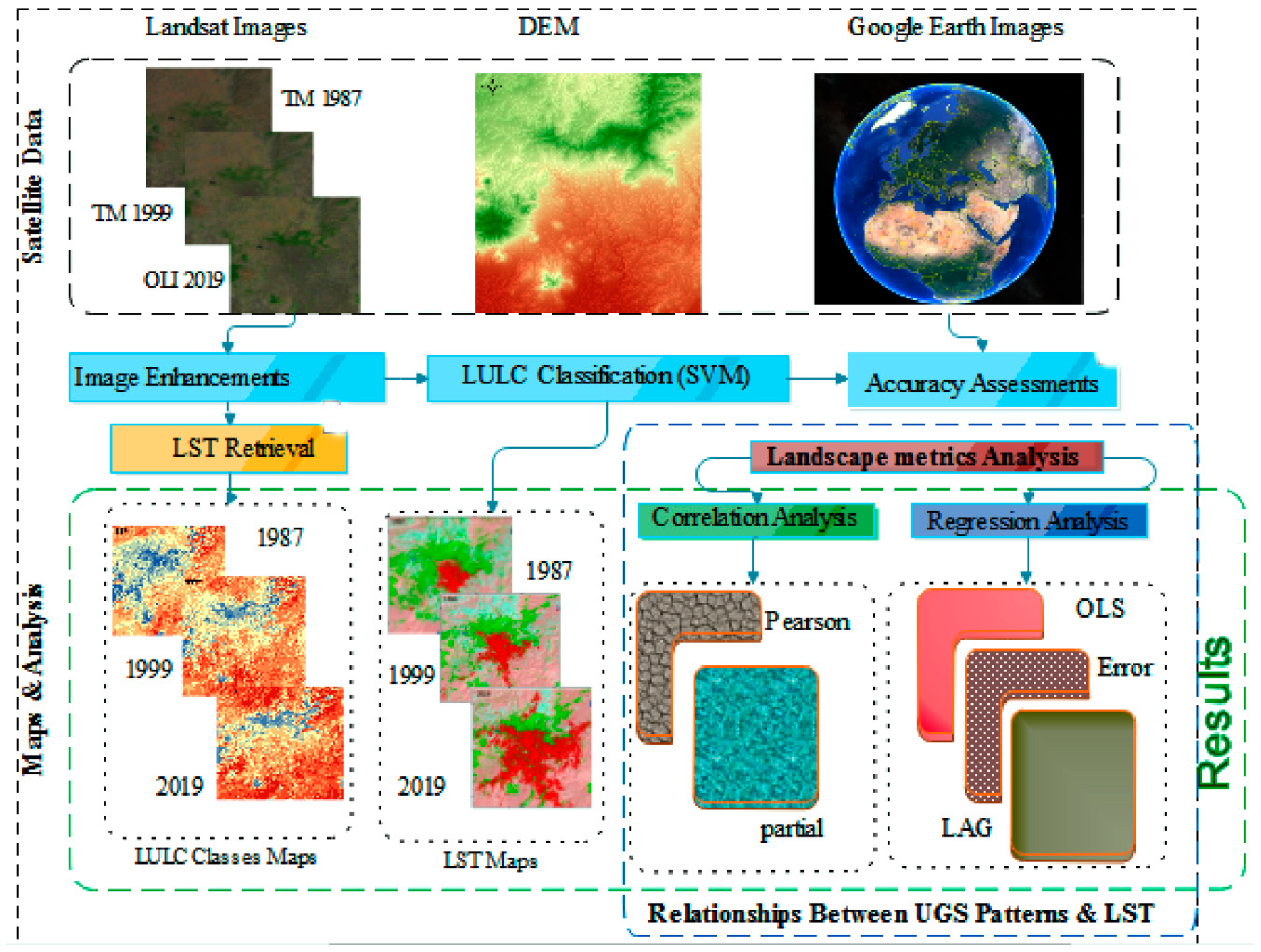
2. Materials and Methods

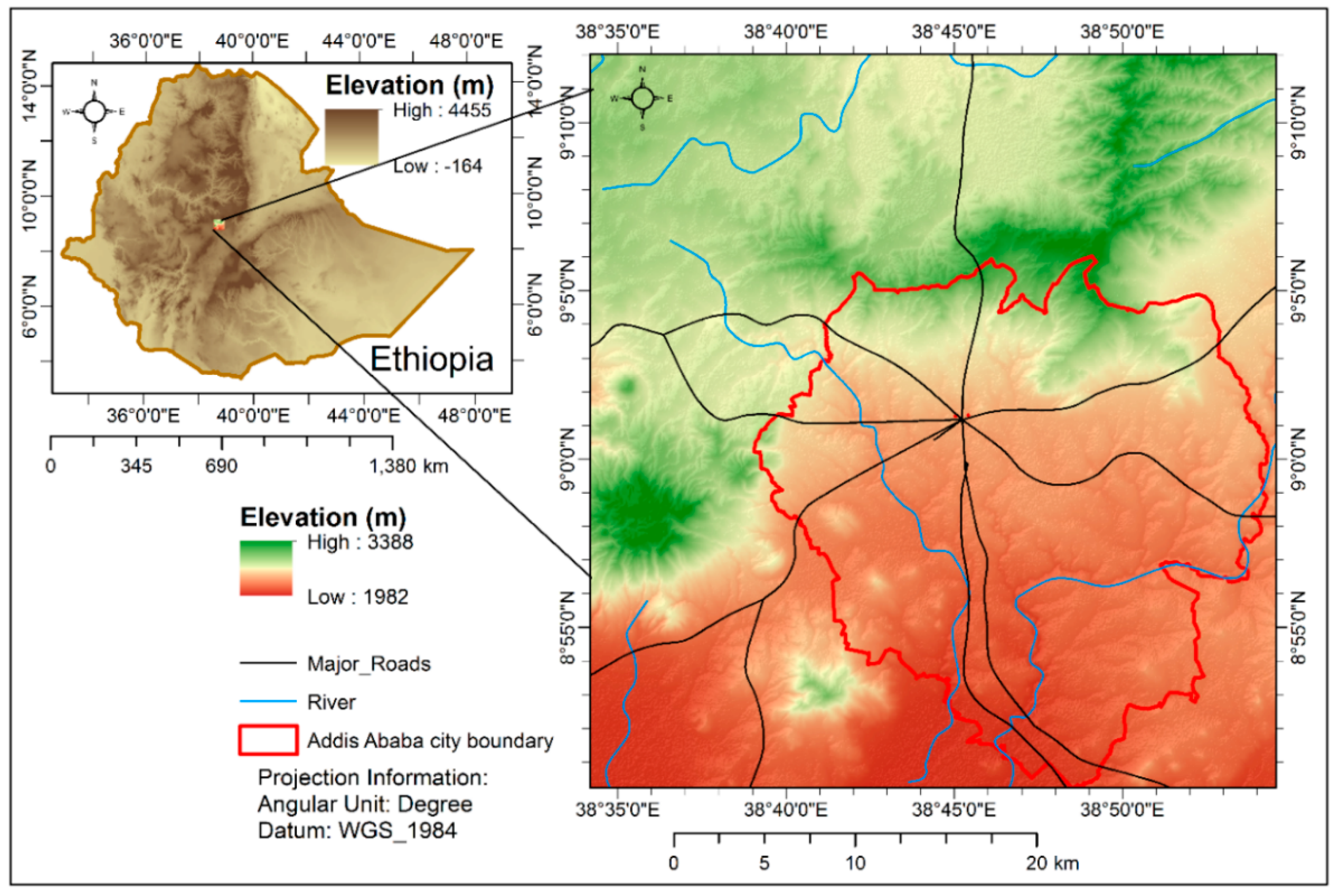
2.1. Study Area

The study area, presented in Figure 1, includes the city of Addis Ababa and its surrounding regions, which cover 1711.74 km². It is located between 8°54′00″ N to 9°8′00″ N and 38°36′00″ E to 38°54′00″ E. The mean altitude of the study site is 2685 m above sea level. Addis Ababa is the capital, and most important commercial, political, and industrial city of Ethiopia. The city also serves as the seat of the African Union in addition to the Oromia National, Regional State. The city has a total area of about 527 km² and 4.3 million residents in the year 2017 [3], which cover 16.9 percent of the country’s urban inhabitants and 3 percent of the country’s overall inhabitants. The city’s population is expected to grow to 5.9 million in 2030 at a mean annual growth rate of 4.1 percent [61]. The climate in the study site is warm and temperate. Typically, March, April, and May are the warmest months of the year, with values of 25 °C for the mean highest temperatures. November and December are the coldest months with the lowest average temperature values of 8 °C. The rainfall is moderate to heavy during the summer (June to August) with a mean yearly rainfall of 1143 mm. The dispersed nature of Addis Ababa city’s spatial growth [3] and the rapid reduction of urban green space [62,63] are likely to have considerable impacts on spatial patterns of temperature [42,51,64]. Hence, Addis Ababa metropolitan area was an interesting case study to explore the environmental effects of urbanization.

2.2. Remote Sensing Data and Processing

Landsat is regularly adopted for computing LST in UHI investigations [43] and is openly available. Three Landsat images for 1987, 1999, and 2019 acquired during the dry season (February) with clear atmospheric conditions were used in this study. These images were chosen based on the availability of the data for the same months. This month (February) was selected based on previous studies that reported the UHI effects during the dry season were more significant [34,59]. The images were downloaded from the United States Geological Survey. The details of the data implemented for the study are shown in

Table 1. Remotely sensed data information for the study sites.

Satellite	Sensor	Path/Row	Acquisition Date	Season	Source
Landsat-5	TM	168/54	1987/02/09	Dry
Landsat-5	TM		1999/02/10		www.earthexplorer.usgs.gov
Landsat-8	OLI/TIRS		2019/02/01
	Digital elevation model (DEM) data (30-m spatial resolution)

. The multispectral bands were applied for classification of land-use/land cover (LULC) classes, while the thermal bands were used to calculate satellite brightness temperatures.

2.3. Land Cover Mapping

The general idea of remotely sensed data and the methodological method employed for this investigation are illustrated in Figure 2 flow diagram.

Satellite data pre-processing, spectral, spatial, and radiometric rectifications were done using standard remote sensing methods [65,66,67]. The study then mapped the LULC classes based on 30 m resolution of Landsat images, bands 5-4-3 for Landsat 8 OLI, and bands 4-3-2 for Landsat-5. Depending on its spectral signature, each pixel in the image was allocated to the category that fits best. Ancillary data, such as Google Earth images, were used to help in classification. The five defined categories were: built-up area, bare land, water body, vegetation cover, and grassland. A supervised classification approach with the support vector machine (SVM) classifier algorithm was employed. The correctness of land cover classified results was validated by the accuracy assessment approaches [68,69,70]. The study further merged the vegetation cover, grasslands, and water body as UGS to analyze the relationships between the spatial patterns of UGS and land LST.

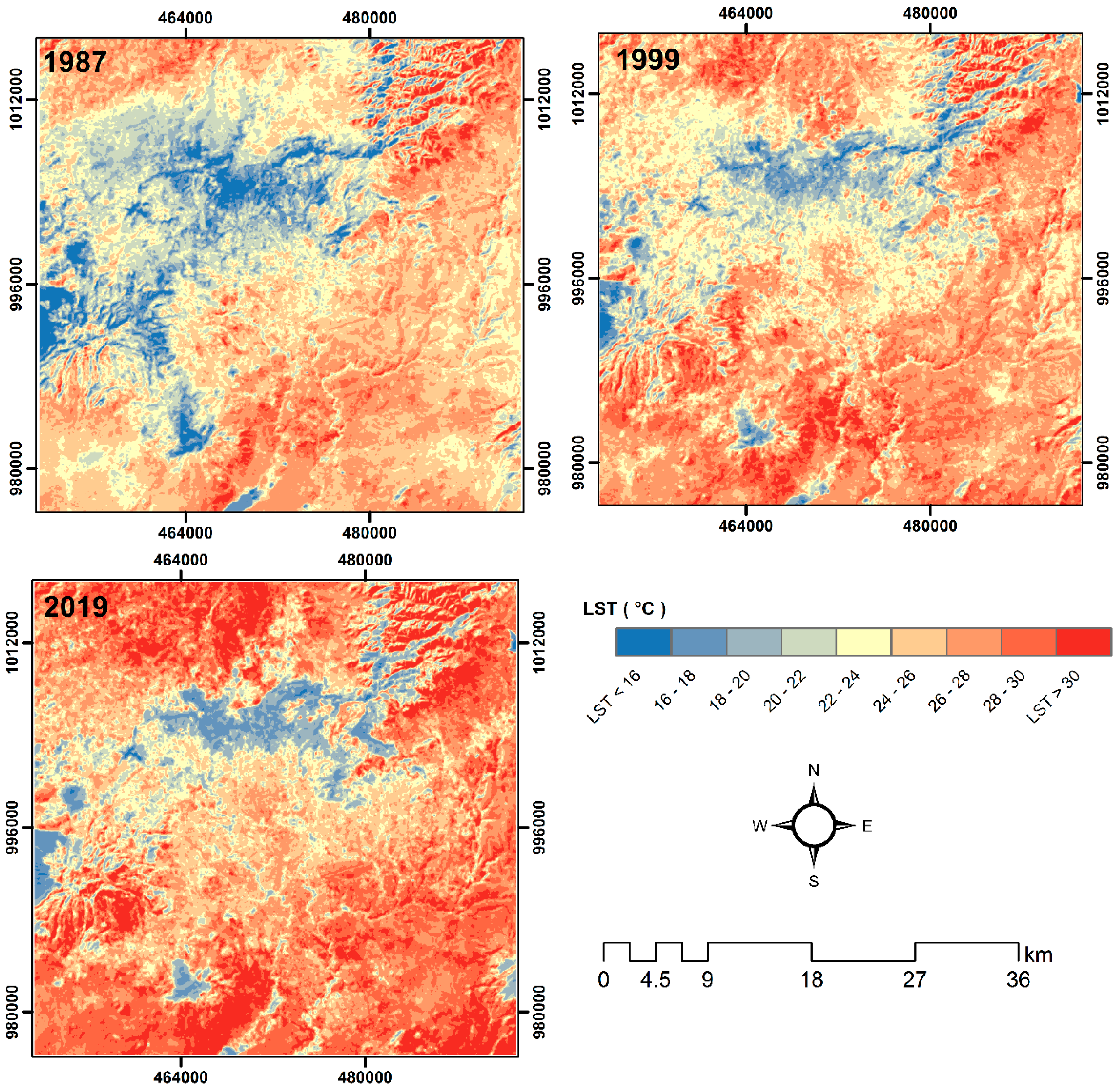
2.4. Land Surface Temperature Retrieval

Several factors affect LST, including surface emissivity [71,72], elevation [19,73], wind velocity, time of day, and the phenomena of precipitation [74], clouds [4,43,72], atmospheric situations, satellite sensor features, and the mathematical approaches used to retrieve LST [75,76]. It is not feasible to explicitly account for all these components in this study due to the following reasons: (1) the atmospheric data are not available before January 2000. (2) Though the atmospheric rectification based on satellite imagery using generic parameters is important, it has been revealed to the result in only a minor error for LST retrieval [77]. (3) This study implemented LST for the exploration of UGS patterns’ effect on urban land temperatures.

2.4.1. Retrieval of Spectral Radiance

To estimate LST, the study used thermal infrared band 6 (10.40–12.50 μm) for Landsat 5-TM and band 10 for Landsat-8 OLI (10.3–11.3 µm) with resolutions of 120 m and 100 m, respectively. As the Landsat images were produced from continuous digital values (digital numbers), to obtain LST, the digital number of pixels for each thermal image was converted to the top-of-atmosphere (TOA) radiance using the Equations (1) and (2) [4,30,64,65]. For Landsat 5-TM (TIR band 6), Equation (1) and for Landsat 8 (TIR band 10), Equation (2) were used as follows:

$${\mathrm{L}}_{\mathsf{\lambda }}=\frac{ {\mathrm{L}}_{\max }-{ \mathrm{L}}_{\min }}{{\mathrm{QCAL}}_{\max }-{ \mathrm{QCAL}}_{\min }}\times \left(\mathrm{QCAL}-{ \mathrm{QCAL}}_{\min }\right)+{\mathrm{L}}_{\min }$$

(1)

where:

(a)

${\mathrm{L}}_{\mathsf{\lambda }}$—TOA Spectral Radiance $\left(\mathrm{W}/\left({\mathrm{m}}^2 \times \mathrm{sr} \times \mathsf{\mu }\mathrm{m}\right)\right)$;

(b)

${\mathrm{LMAX}}_{\mathsf{\lambda }}$—the spectral radiance (QCALMAX ($\mathrm{W}/({\mathrm{m}}^2 \times \mathrm{sr} \times \mathsf{\mu }\mathrm{m})$));

(c)

${\mathrm{LMIN}}_{\mathsf{\lambda }}$—the spectral radiance (QCALMIN $\left(\mathrm{W}/\left({\mathrm{m}}^2 \times \mathrm{sr} \times \mathsf{\mu }\mathrm{m}\right)\right)$);

(d)

${\mathrm{LMIN}}_{\mathsf{\lambda }}$ = 1.238; ${\mathrm{LMAX}}_{\mathsf{\lambda }}$ = 15.303;

(e)

QCAL—the quantized rectified pixel value in Digital Numbers (DN); and

(f)

QCALMAX and QCALMIN the—maximum and minimum quantized adjusted pixel values matching to${ \mathrm{LMAX}}_{\mathsf{\lambda }}$ in DN = 255 and ${\mathrm{LMIN}}_{\mathsf{\lambda }}$ in DN = 1, respectively.

$${\mathrm{L}}_{\mathsf{\lambda }} ={ \mathrm{M}}_{\mathsf{\lambda }}\times { \mathrm{QCAL}}_{\mathsf{\lambda }} +{ \mathrm{A}}_{\mathsf{\lambda }}$$

(2)

where, ${\mathrm{M}}_{\mathsf{\lambda }}$ and ${\mathrm{A}}_{\mathsf{\lambda }}$ = Radiance multiplicative and additive scaling factor for the band, respectively, and ${\mathrm{QCAL}}_{\mathsf{\lambda }}$= the quantized calibrated pixel value in DN. The study then converted the ${\mathrm{L}}_{\mathsf{\lambda }}$ values to at-satellite brightness temperature (TB) using (Equation (3)).

$${\mathrm{T}}_{\mathrm{B}}=\frac{{\mathrm{K}}_2}{\ln \left( \frac{{\mathrm{K}}_1}{{\mathrm{L}}_{\mathsf{\lambda }}}+1\right)}$$

(3)

where, TB values in Kelvin (K); K1, K2 = Thermal conversion constants for the band.

2.4.2. Estimation of the Land Surface Emissivity

Land surface emissivity (ε) is one of the essential parameters in retrieving LST. Surface materials have different emissivity due to their different viewing angles, materials, and roughness. Normalized difference vegetation index (NDVI) is one of the most commonly applied vegetation indexes. NDVI is calculated from the red (R) and near-infrared (NIR) bands—for Landsat 5, and 8, using Equation (4).

$$\mathrm{NDVI} = \frac{\mathrm{NIR} - \mathrm{RED}}{\mathrm{NIR} + \mathrm{RED}}$$

(4)

where, RED is a red spectral band, and NIR is a near-infrared spectral band of Landsat images. Hence, to compute the LSE, the NDVI-based emissivity approach proposed by Van de Griend and Owe [78] was applied in this study (Equation (5)).

$$\mathsf{\epsilon } ={ \mathsf{\epsilon }}_{\mathrm{v}}{\mathrm{P}}_{\mathrm{v}}+{\mathsf{\epsilon }}_{\mathrm{s}}\left(1 -{ \mathrm{P}}_{\mathrm{v}}\right)+{\mathrm{d}}_{\mathsf{\epsilon }}$$

(5)

where, ${\mathsf{\epsilon }}_{\mathrm{s}}{ \mathrm{and} \mathsf{\epsilon }}_{\mathrm{v}}$ denote the emissivity of bare soil pixels and vegetation, respectively. Where ${\mathrm{P}}_{\mathrm{v}}$ indicates the fraction of vegetation [79], which was calculated using Equation (6):

$${\mathrm{P}}_{\mathrm{v}}={\left[\frac{ \mathrm{NDVI} -{ \mathrm{NDVI}}_{\min }}{{\mathrm{NDVI}}_{\max } -{ \mathrm{NDVI}}_{\min }}\right]}^2$$

(6)

In the above, ${\mathrm{NDVI}}_{\min }$and ${\mathrm{NDVI}}_{\max }$ are 0.2 and 0.5, respectively in a universal condition [80]. The term ${\mathrm{d}}_{\mathsf{\epsilon }}$includes geometrical distribution influence of the internal reflections and natural surface. As suggested by Valor and Caselles [81], the values of ${\mathsf{\epsilon }}_{\mathrm{s}}$and ${\mathsf{\epsilon }}_{\mathrm{v}}$ are 0.960 and 0.985, respectively, for vegetation structures and unknown emissivity. The study also applied these emissivity values in the calculation. Moreover, for rough and heterogeneous surfaces, ${\mathrm{d}}_{\mathsf{\epsilon }}$can increase to 2% of emissivity [80] and the values of ${\mathrm{d}}_{\mathsf{\epsilon }}$are calculated as proposed by Sobrino et al. [82], using Equation (7):

$${\mathrm{d}}_{\mathsf{\epsilon }} = \left(1 -{\mathsf{\epsilon }}_{\mathrm{s}}\right)\left(1 -{ \mathrm{P}}_{\mathrm{v}}\right)\times \mathrm{F} \times { \mathsf{\epsilon }}_{\mathrm{s}}$$

(7)

where, F is a shape factor with a mean value of 0.55, assuming different types of geometrical distributions [82]. Finally, the rectified land surface temperature maps (Figure 3) were produced using the Equation (8) as:

$$\mathrm{LST}=\frac{{\mathrm{T}}_{\mathrm{B}}}{\left(1+ \mathsf{\lambda } \left( \frac{{\mathrm{T}}_{\mathrm{B}}}{\mathrm{p}} \right) \times \ln \left[\mathsf{\epsilon }\right]\right)}$$

(8)

where, LST = the Land Surface Temperature in Kelvin (K);$\mathrm{p} = \mathrm{hc}/\mathrm{k} (1.438 \times {10}^{-2} \mathrm{mk}$); h = Planck constant ($6.626 \times {10}^{-34}{\mathrm{J} \mathrm{s}}^{-1}$), and c = velocity of light ($2.998 \times 108{ \mathrm{ms}}^{-1}$); k = Boltzmann constant ($1.38 \times {10}^{-23}-{\mathrm{J} \mathrm{K}}^{-1}$), and λ = the wavelength of emitted radiance. To obtain the LST values in Celsius (°C), 273.15 was subtracted from the original values (K). All steps were carried out by developing a raster calculator model using ArcGIS version 10.4.1.

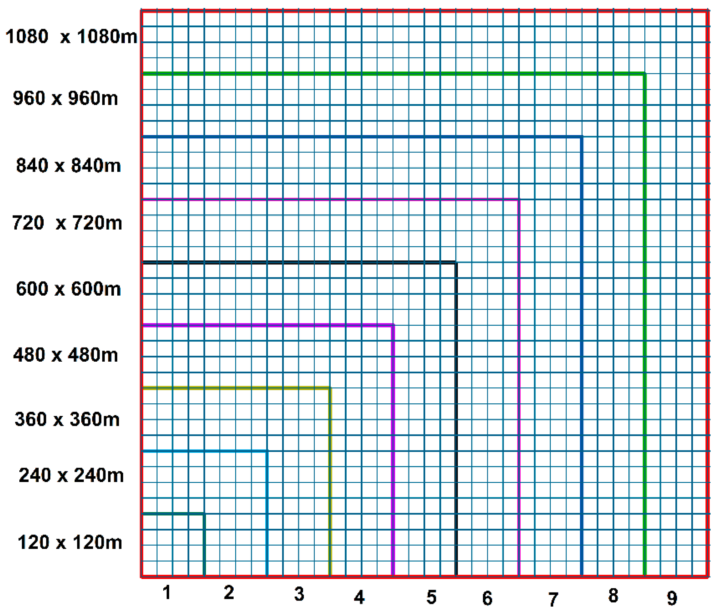
2.5. The Spatial Pattern of Urban Green Space Analysis

Four landscape metrics: (1) Percent cover of green space (PGS) (among composition metrics), and three configuration metrics: (2) patch density (PD), (3) edge density (ED), and (4) mean nearest-neighbor distance (MNN) (

Table 2. Chosen landscape metrics implemented from McGarigal [83].

Metric	Formula	Units	Narrative
Percent of urban green spaces (PGS) (%)	PGS = ${\mathrm{p}}_{\mathrm{i}}$= $\frac{{{\displaystyle \sum }}_{\mathrm{j}=1}^{\mathrm{m}}\mathrm{aji}\left(100\right)}{\mathrm{A}}$	Percent	${\mathrm{p}}_{\mathrm{i}}$ = share of the landscape occupied by patch type (class) i. A = area of entire landscape (m2).
Patch density (PD)	$\mathrm{PD}=\frac{{\mathrm{n}}_{\mathrm{i}}}{\mathrm{A}}\left(\mathrm{10,000}\right)\left(100\right)$	Number/100 hectares	${\mathrm{n}}_{\mathrm{i}}$ = number of patches in the landscape of patch type (class) i.
Edge density (ED)	$\mathrm{ED}=\frac{{{\displaystyle \sum }}_{\mathrm{k}=1}^{\mathrm{m}}{\mathrm{e}}_{\mathrm{ik}}}{\mathrm{A}}\left(\mathrm{10,000}\right)$	Meter/hectare	eik = whole length (m) of edge in landscape containing patch type (class) i.
Mean nearest-neighbor distance (MNN)	$\mathrm{MNN} ={ \mathrm{h}}_{\mathrm{ij}}$	Hectare	${\mathrm{h}}_{\mathrm{ij}}$ = distance (m) from patch ij to closest adjoining patch of the same type (class).

) were applied to compute the spatial patterns of UGS. These metrics denote the main characteristics that can describe the spatial patterns of UGS, including composition, complexity, configuration, and fragmentation of patches. These metrics were chosen based on their prevalence in the scientific literature and environmental significance [2,16,39,49,53]. The spatial metrics are sensitive to scales in the spatial pattern explorations [16,45,57]. The dependency on the scale also impacts on the results of UGS and LST analysis [16,45]. Thus, the study used 9 varied sizes of analytical units starting from 120 m (which is equal to the pixel size of the TM thermal band) to 1080 m. Accordingly, 120 m × 120 m, 240 m × 240 m, 360 m × 360 m, 480 m × 480 m, 600 m × 600 m, 720 m × 720 m, 840 m × 840 m, 960 m × 960 m, and 1080 m × 1080 m (Figure 4) were applied to determine the effects of spatial scale and distinguish the optimum spatial size in the UGS and LST relationship analysis. The study then calculated the chosen metrics and the values over generated grids using the Patch Analyst extension in ArcGIS. The LST for every analytical unit was computed using the developed-in Zonal Statistic tool of ArcMap ArcMap 10.4.1.

2.6. Statistical Analysis

2.6.1. Correlation Analysis

A Pearson correlation matrix was built based on the correlation between LST and the spatial patterns of the UGS. A partial correlation analysis was performed to assess the configuration metrics (PD, ED, and MNN) and the LST by controlling for the influence of the PGS. Controlling for the influence of PGS is important, as it had the highest correlation with the configuration metrics as well as the LST across the study period in almost all tested spatial scales. Thus, the Pearson correlation evaluation is reliable to get a spurious connection between configuration metrics and LST.

2.6.2. Regression Analysis

For each of the studied period, multiple regression models were built to select the best model that describes the highest variance in LST. To avoid redundancy (inter-correlation) within the chosen spatial metrics [43,84], a multi-collinearity condition number (MCN) coupled with the variance inflation factor (VIF), for each metric was calculated. The values of MCN and VIF for each independent variable were less than 30 and 7.5, respectively, which is acceptable for modeling [43].

The study then employed the ordinary least squares (OLS) for every built model, with the assumption of independent error terms. OLS is usually the initial step for diagnostic and to use as a benchmark for comparison. This method neglected the issue of spatial autocorrelation [45,53]. Spatial data contains spatial dependence and heterogeneity from spatial autocorrelation, which can amplify confounding in the analysis. Spatial clustering in error may come from spatial heterogeneity or spatial dependence. To address this, spatial auto-regression (SAR) models that incorporated spatial autocorrelation into the modeling are more suitable to explore the association between spatial patterns of UGS and LST [43,45,85]. Regarding SAR, the neighborhood interconnection of the response variable was estimated by a (n × n) framework of spatial weights and was incorporated in the ordinary multiple linear regression to consider spatial autocorrelation [86]. Accordingly, two spatial regression approaches: spatial lag and error models were applied to investigate the impacts of the spatial pattern of UGS on LST. The spatial lag model expects that the spatial autoregressive occurs only in the response variable [86]. The spatial lag model is expressed in Equation (9).

$$\mathrm{y} = \mathsf{\rho }\mathrm{Wy} + \mathsf{\beta }\mathrm{X} + \mathsf{\epsilon }$$

(9)

where Wy is the spatial lag variable, $\mathsf{\rho }$ is a spatial autoregressive coefficient, X is the independent regression variable, β is the regression coefficients, and ε is the error term vector.

Conversely, the spatial error model considers the spatial impacts that are not wholly defined by the factors within the error terms and is presented in Equation (10).

$$\mathrm{y}= \mathsf{\beta }\mathrm{X} + \mathsf{\lambda }\mathrm{W}\mathsf{\mu } + \mathsf{\epsilon }$$

(10)

where Wμ is a vector of spatially lagged errors, and λ is a coefficient of spatial autoregressive

The study implemented the Lagrange Multiplier statistics to match the applied modeling methods for each year. The standard coefficients (beta weights) were used to examine the relative significance of composition and configuration metrics on estimating LST [43,45]. The regression model was run using GEODA version 1.8.16 [87].

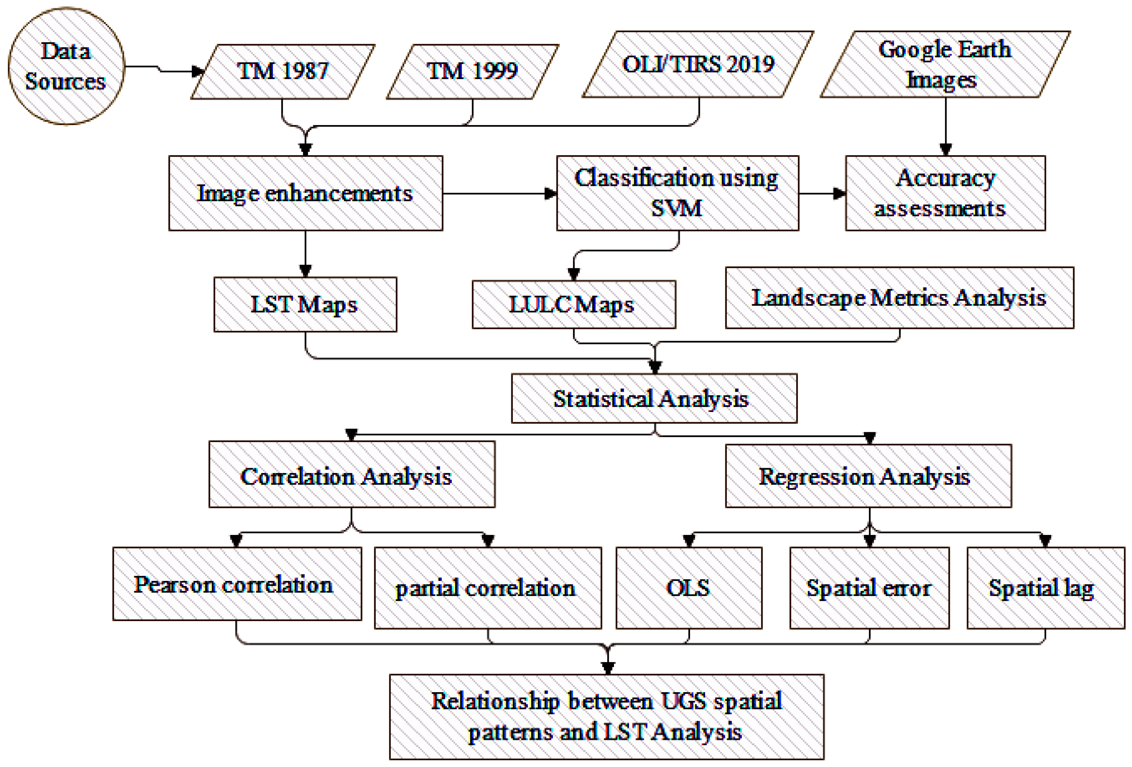
2.7. Summary of Experimental Steps

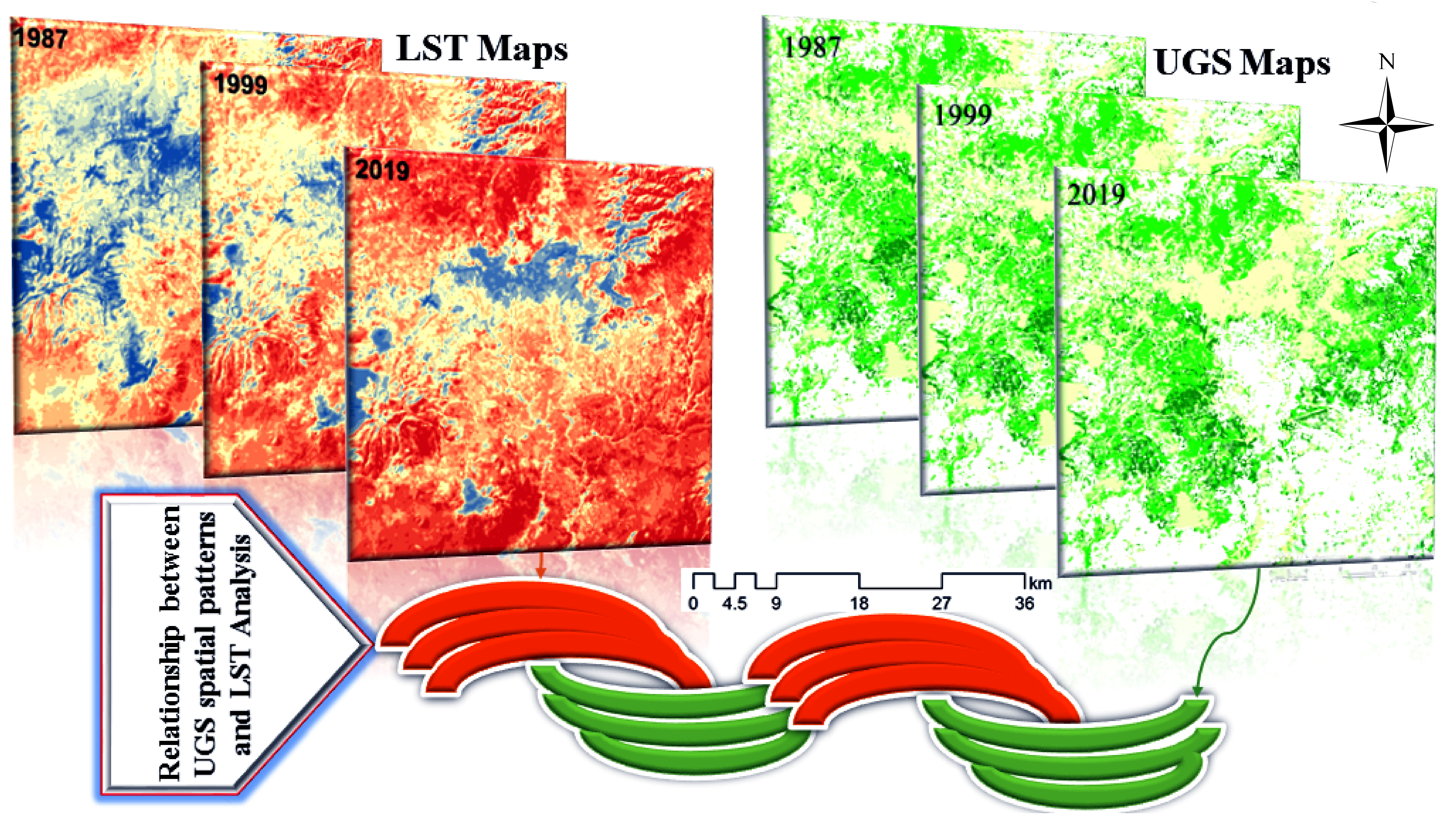
Figure 5 illustrates three series of tasks that were conducted to analyze the spatial patterns of UGS and LST. These are (1) classification of the LULC and validation process; (2) LST analysis; and (3) examining the effects of UGS patterns on the LST.

3. Results

3.1. LULC Changes in Addis Ababa Metropolitan Regions

Figure 6 shows the changes in the land use pattern of the Addis Ababa metropolitan regions from the 1987 to 2019 study period. The area of non-urban areas (vegetation, grass, agriculture, and water) has rapidly been reduced across the study periods. In contrast, the area of the urban region has significantly increased over the past 32 years (Figure 6). The overall and kappa coefficients of LULC classes were 87.8, 88.2, and 89.4 in 1987, 1999, and 2019, respectively. The kappa values were 0.85 for 1987 and 1999, respectively, and 0.88 for 2019. These values indicated that the generated data had responsibly high accuracy.

3.2. Space and Time-Based Pattern of UGS in the Addis Ababa Metropolitan Area

Table 3. Landscape metrics results from 1987 to 2019.

Metrics	Unit	1987	1999	2019
PGS	%	44.33	38.36	26.31
PD	Number/100 ha	5	7	27
ED	m/ha	96.30	111.39	215.14
MNN	m	42.00	57.88	91.36

shows the relative change patterns of UGS and the corresponding landscape metrics. The proportion of urban green space (PGS) in Addis Ababa metropolitan decreased gradually from 44.3% in 1987 to 33.4% in 1999, followed by a considerable decrease to 26.3% in 2019 (Table 3). In terms of fragmentation and aggregation, the PD values of the UGS gradually increased between 1987 and 1999, and then sharply increased further in 2019. The result indicated that the UGS was disaggregated across the study periods, but UGS patch fragmentation was more significant in 2019, as evidenced by a sharp rise in the PD values: 7 in 1999 to 27 in 2019. The shape complexity of UGS, which was calculated by ED, revealed that changes in the overall complexity of the patches became more complex and irregular patterns from 1987 to 2019. This trend was high during the 1999–2019 periods, as evidenced by a rapid increase in the ED values, from 111.4 m/ha in 1999 to 2015.1 m/ha in 2019 (Table 3). Whereas, the connectivity among UGS patches increased notably from 1987 to 2019 and was generally increased by 41 m during this study period (from 42 m of MNN in 1987 to 91.36 m in 2019) (Table 3).

In general, it was inferred that Addis Ababa lost its green space from 1987 to 2019, at about 12% between 1999 and 2019. Concerning the spatial patterns, UGS patches have become smaller, more complex in shape, and more fragmented overall.

3.3. Effects of Spatial Patterns of UGS on LST

Across the study periods, the Pearson correlation analysis revealed that most metrics were significant at all analytical units, except MNN at large spatial scales (

Table 4. Correlation coefficients between Landscape metrics and LST. The bold rows indicate the partial correlation analysis, where for proportion of urban green space (PGS), the control variables were the configuration metrics, and for configuration metrics, the control variable was PGS.

Year	Variable	Scale
		120 m	240 m	360 m	480 m	600 m	720 m	840 m	960 m	1080 m
1987	PGS	−0.658 **	−0.647 **	−0.661 **	−0.610 **	−0.529 **	−0.509 **	−0.449 **	−0.427 **	−0.470 **
		−0.465 **	−0.347 **	−0.305 **	−0.300 **	−0.298 **	−0.146 *	−0.103	−0.179 *	−0.175 *
	PD	0.570 **	0.625 **	0.631 **	0.598 **	0.503 **	0.552 **	0.467 **	0.375 **	0.429 **
		0.259 **	0.282 **	0.230 **	0.267 **	0.205 **	0.277 **	0.219 **	0.019	0.001
	ED	−0.484 **	−0.536 **	−0.586 **	−0.513 **	−0.417 **	−0.447 **	−0.418 **	−0.380 **	−0.410 **
		0.209 **	0.161 *	0.077	0.166 *	0.192 *	0.089	0.077	0.032	−0.018
	MNN	0.392 **	0.350 **	0.194 **	0.038	0.119	0.087	0.016	0.020	0.050
		0.103	0.105	−0.008	−0.076	−0.078	−0.028	−0.135	−0.022	0.052
1999	PGS	−0.649 **	−0.686 **	−0.606 **	−0.566 **	−0.514 **	−0.555 **	−0.530 **	−0.468 **	−0.420 **
		−0.483 **	−0.468 **	−0.376	−0.337 **	−0.305 **	−0.394 **	−0.235 **	−0.289 **	−0.279 **
	PD	0.548 **	0.581 **	0.519 **	0.482 **	0.453 **	0.449 **	0.501 **	0.406 **	0.352 **
		0.282 **	0.214 **	0.148	0.129	0.113 *	0.071	0.131	0.021	−0.002
	ED	−0.414 **	−0.492 **	−0.466 **	−0.457 **	−0.397 **	−0.405 **	−0.450 **	−0.346 **	−0.325 **
		0.194 **	0.183 **	0.126	0.112 *	0.143 *	0.188 *	0.104	0.108	0.133
	MNN	0.262 **	0.398 **	0.142 *	0.111 *	0.146 *	0.055	0.067	0.104	−0.004
		0.023	0.144 *	−0.045	−0.079	−0.001	−0.102	−0.042	0.006	−0.042
2019	PGS	−0.797 **	−0.823 **	−0.769 **	−0.708 **	−0.733 **	−0.652 **	−0.613 **	−0.551 **	−0.490 **
		−0.613 **	−0.580 **	−0.487 **	−0.410 **	−0.400 **	−0.246 **	−0.249 **	−0.253 **	−0.098
	PD	0.740 **	0.708 **	0.649 **	0.612 **	0.649 **	0.598 **	0.580 **	0.504 **	0.494 **
		0.466 **	0.245 **	0.172 *	0.177 *	0.195 *	0.122 *	0.195 *	0.058	0.111
	ED	−0.623 **	−0.673 **	−0.645 **	−0.587 **	−0.624 **	−0.550 **	−0.562 **	−0.477 **	−0.436 **
		0.118 *	0.053	0.002	0.037	0.054	0.065	0.126	0.045	−0.004
	MNN	0.294 **	0.308 **	0.139 **	0.209 **	0.120 *	0.098	−0.069	0.054	0.053
		0.026	0.050	−0.023	−0.030	−0.018	−0.064	−0.019	0.022	0.027

** p < 0.01, * p < 0.05.

). Composition metrics (PGS) showed a negative correlation with LST, suggesting that the more UGS patches give a higher cooling effect. Among the configuration metrics, PD revealed a positive correlation with LST, indicating that the low fragmented UGS patches show a more effective cooling signature. In contrast, the ED had a negative correlation with LST across all analytical units. In contrast, MNN revealed a positive, significant correlation with LST only at analytical units of 120 m, 240 m, and 360 m. Similar to PGS, the intensity of the correlations between the three configuration metrics (PD, ED, and MNN) and LST also generally decreased with the increase of the analysis scale.

After controlling for the impact of PGS, the correlations (i.e., partial correlations) between LST and configuration metrics were significantly changed and are shown in Table 4. From the table, four features were notable: (i) the intensity of the partial correlations, calculated by the correlation coefficients significantly declined relative to their equivalent Pearson correlation coefficients. (ii) Some configuration metrics and LST became insignificant (e.g., MNN). (iii) Significantly correlated at only smaller scales (e.g., ED was significantly correlated to LST at less than or equal to 360 m, and reduced as the spatial magnitude increased), and (iv) More importantly, the association between some configuration metrics and LST shifted their directions. For instance, the correlation between MNN and LST were shifted from positive to negative when the analytical unit was between 360 and 960 m, 360 to 840 m, and 360 to 840 m in the year 1987, 1999, and 2019, respectively. In addition, the correlation of ED with LST was shifted from negative to positive across all analytical units except at 1080 m in the year 1987.

3.4. Influences of UGS Spatial Size Pattern on LST

The correlation between the implemented landscape metrics and LST appears to be regularly decreasing with spatial size (Table 4). Whereas, some configuration metrics can influence on LST separately of the composition metrics at smaller scales. For example, the correlation of PD continued to be significant with LST at analytical units between 120 m to 600 m. This tendency is also noted when considering the influence of PGS across the study periods. The results imply that the patch density has a more prominent effect on LST than the other configuration metrics at smaller scales. It is noted that the optimum spatial scale of UGS for exploring the relationship between LST and spatial metrics could be between 120–600 m.

Indeed, this study did not find nor does it seem feasible to precisely identify a scale at which the correlation between LST and metrics converge. However, most metrics were generally more predictable at 240 m. For instance, after controlling for the impact of composition metrics (PGS), connectivity between the green spaces revealed a significant positive effect on LST only on the spatial scale of 240 m, as evidenced by MNN values in Table 4. Thus, 240 m × 240 m was applied as the optimum size for further analysis.

3.5. The Relative Significance of Composition and Configuration of UGS on LST

Table 5. Results for regression modeling. The Z-value shows the relative implication of each variable in the model. R² (coefficient of determination) and AIC (Akaike info criterion) reveal the general enactment of each model.

Year	Model	Variable	Coefficient	R2	Z-Value	AIC
1987	Spatial error	PGS	−2.814 **	0.482	−4.620	831.739
		ED	3.589 **		2.833
		PD	0.203 **		3.809
		MNN	0.001 *		2.259
	Spatial LAG	PGS	−2.822 **	0.480	−4.572	831.379
		ED	3.409 **		2.833
		PD	0.217 **		4.061
		MNN	0.001 *		2.172
	OLS	PGS	−3.197 **	0.463	−5.157	835.587
		ED	3.252 **		2.499
		PD	0.196 **		3.565
		MNN	0.001 *		2.054
1999	Spatial error	PGS	−4.226 **	0.584	−8.091	829.129
		ED	4.654 **		3.929
		PD	0.152 **		3.783
		MNN	0.001		1.372
	Spatial LAG	PGS	−3.916 **	0.565	−7.432	836.386
		ED	4.187 **		3.558
		PD	0.145 **		3.419
		MNN	0.001		1.564
	OLS	PGS	−0.188 **	0.507	−7.494	854.861
		ED	3.131 *		2.471
		PD	0.125 **		2.726
		MNN	0.001		1.627
2019	Spatial error	PGS	−4.517 **	0.661	−7.571	530.529
		PD	0.121 **		2.914
		ED	0.442		0.472
		MNN	0.0003		0.7335
	Spatial LAG	PGS	−4.481 **	0.655	−7.460	531.278
		PD	0.121 **		2.928
		ED	0.640		0.667
		MNN	0.0002		0.5667
	OLS	PGS	−4.468 *	0.634	−7.081	536.774
		PD	0.118 **		2.705
		ED	0.201		0.203
		MNN	0.0002		0.6108

** p < 0.01, * p < 0.05.

shows that the results from spatial error, Lag, and OLS linear regression models, the PGS had significant negative impacts on LST, across all the study periods. Additionally, PGS was the most significant indicator of LST, playing a considerably more significant role in forecasting LST relative to the other spatial configuration factors (Table 5). Among the three configuration metrics, PD played a much more significant and positive effect in estimating LST (Table 5). Other metrics, ED and MNN had positively significant effects on LST in the years 1985 and 1999.

The results indicated that composition, fragmentation, and shape complexity characteristics of UGS spatial patterns affected LST. Moreover, the results showed that the spatial error model outperformed its correspondent Lag, and OLS models, for each of the periods. This was evidenced by the higher R² values and the lower AIC of the spatial error model compared to the other two models (Table 5).

4. Discussion

The relative importance of both spatial composition and configuration of UGS on LST was almost similar across the study periods. PGS was the critical factor in estimating LST. This is consistent with prior studies that suggested that the amount of green space plays a more important role in the cooling effects of the city than their configurations [42,45,46,85]. The overall results suggest that the fraction of green patches, their geometrics shape, degree of aggregation and fragmentation, and the proximity distance of patches to each other, are the main determinants of LST in urban regions. In other words, for the greater cooling effect, more patches of UGS distribution and a reasonable spatial configuration are important considerations to impact LST and reduce the urban heat.

4.1. Scale-Dependence of UGS Spatial Patterns and LST Relationships

The association between PGS and LST was negative at all spatial scales, across the study periods. This is consistent with the past results that showed that the amount of vegetation cover is a significant feature in mitigating UHI effects [32,45,53]. The study also found that increasing the spatial scale, the relationship between landscape metrics and LST, including both composition and configuration, becomes weaker, highlighting a scale effect. The results are consistent with the recent studies found elsewhere [46]. Furthermore, a nonlinear relation is noted between LST and vegetation cover- the LST reduction by enhancing the amount of vegetation cover was relatively lower at larger scales (

Table 6. Results from OLS linear regression. The effects of UGS on LST was predicted by PGS.

Year		Scale
		120 m	240 m	360 m	480 m	600 m	720 m	840 m	960 m	1080 m
1987	Coef.	−0.894 **	−0.508 **	−0.507 **	−0.573 **	−0.605 **	−0.307 *	−0.230 *	−0.469 *	−0.428 *
	R2	0.486	0.475	0.467	0.419	0.303	0.320	0.241	0.184	0.225
1999	Coef.	−0.602 **	−0.633 **	−0.621 **	−5.133 **	−4.158 **	−4.158 **	−2.996 **	−0.660 **	−0.728 **
	R2	0.470	0.510	0.384	0.335	0.286	0.333	0.298	0.237	0.195
2019	Coef.	−0.585 **	−0.219 **	−0.640 **	−0.599 **	−0.626 **	−0.587 **	−0.647 **	−0.507 *	−0.268 *
	R2	0.726	0.707	0.606	0.518	0.556	0.441	0.401	0.312	0.258

** p < 0.01, * p < 0.05.

). This is likely due to higher diversity in green features of land covers and complex combinations typically occurring with the higher green cover than for small scales. Hence, smaller green fractions are likely less sensitive to the effect of changes in the proportion of vegetation cover on LST.

As noted, while the study did not find the exact spatial scale at which the greatest correlation has occurred, but it appeared that most metrics became more predictable at 240 m. This could be a robust feature considering the following three reasons, as demonstrated in this study. Primarily, after controlling for the effects of PGS, patch density of UGS revealed significant positive impacts on LST at the spatial extents between 120 m and 600 m in each studied period (see Table 4). Secondly, after controlling for the impact of composition metrics, connectivity between the green spaces revealed a significant positive effect on LST only on the spatial scale of 240 m in the year 1999, as evidenced by MNN values in Table 4. Third, such spatial scales were also suggested in earlier studies [28,43,57,58], though varied data used and approaches applied. Together this suggests that a spatial scale around 240 m could be an optimal spatial size to investigate the connection between UGS spatial patterns and LST.

The study results also revealed that spatial autocorrelation affected the association between LST and landscape metrics. Results from the spatial error and spatial lag models were higher than OLS in terms of R², regression coefficients, and AIC values. This indicated that temperature in a specific region was affected by and affected the temperature in its surrounding samples (via advection). A similar finding was also suggested by [45,85]. The findings indicated that the LST at a location was not only dependent on the spatial arrangement of UGS in that region but also broader distribution in nearby areas.

4.2. The Spatial Composition and Configuration of UGS Effects on LST

While the amount of urban green space was the critical reason for cooling urban LST, urban greens arrangement was also associated with LST distributions. Arrangement of green space, including patch density, patches connectivity, shape complexity, and edge density, revealed positive effects on LST. These spatial configurations of urban green spaces’ effects on LST; however, varied with the earlier studies in terms of significance, direction, and magnitude. The positive association between PD and LST in this study, for instance, is consistent with studies [42,53,85], suggesting aggregated greenspace is better than a fragmented greenspace in reducing LST, while others reported the opposite [16,49,51]. This study found that all analytical units revealed a positive correlation of the green space patch density with LST. In addition, after controlling for the effects of a green space percent, the PD was positively significant to LST within 120–600 m across the study periods. Similarly, the contradictory results of UGS configuration effects on the LST in different cities were documented by several studies. Edge density of UGS, for instance, was found to be negatively associated with LST in Kansas, USA [42], Baltimore, USA [45], and Berlin, Germany [52], but positive in Singapore [53]. Rising of the edge density may potentially result in a rise of shade offered by vegetation to adjoining surfaces [51,85]. It may also increase energy flow and coupling between vegetation and their neighboring areas [56]. Thereby, taking into account only the process of shading, rising edge density will result in lower LST. Conversely, high edge density is mostly a result of more disaggregated UGS. As small and dispersed UGS has a higher temperature than that of aggregated and larger patches [43,53], which can decrease the effectiveness of surface albedo and evapotranspiration. This study also highlighted that the edge density of UGS had positive effects on LST across the study periods, suggesting that the complex shape and irregular patches of green spaces, the higher in LST. In other words, the UGS with simpler and regular patches leads to reduced LST.

The inconsistent results of configuration metrics reported by different researchers are likely due to the amount of UGS considered in the studies. For instance, in 1987, the amount of UGS was 44.3%. This figure reduced to 38.4% in 1999 and finally reached 26.3% in 2019 (see Table 3). At the same time, the effects of configuration metrics were changed in terms of direction, significance, and magnitude. For instance, the average nearest distances among each patch of UGS had a positive impact on LST in 1987 (see Table 4). However, in the case of data for 2019, it revealed insignificant, even changed its direction to negative at larger scales (see Table 4). This suggests that the amounts of green spaces can decide the effectiveness of configuration metrics to predict the relationship between LST and UGS patterns. Simultaneously, high fragmentation, complex shape pattern, and decreasing the connectivity among each patch observed in 2019 than the other periods. This may suggest that when patches are highly complicated and disconnected, the configuration’s role could be declined. These outcomes can improve the understanding of the irregularity impacts of the spatial configuration of UGS on LST from earlier studies.

Furthermore, the irregularity impacts of configuration metrics on LST could be due to the spatial scale effects. The effects of configuration metrics were variable across the study periods. The average nearest distance between patches (MNN) was, for instance, notable in scale dependence with LST, where the relationships of MNN shifted from positive at a smaller spatial size to negative at the larger spatial size (see Table 4). That is, the correlation between configuration patterns of UGS and LST was sensitive to the spatial scales. The multi-scale analysis can assist resolve these inconsistencies. By exploring the relationship between UGS and LST pattern metrics under various analytical units, the insight into the impacts of UGS patterns on LST can be enhanced.

In general, considering the significant impacts of spatial size [16,28,43,45], the satellite image resolution [42,55], and the choice of statistical approach [51,57], comparing the UGS and LST relations across the studies could be challenging. This multi-scale and multi-year analysis with medium-resolution thermal data assists the interpretation and extension of prior that considered a single snapshot data in multiple cities, e.g., [39,45]. This could have the potential to identify the spatial composition and configuration relationships with LST due to its multiple periods in the same area to confirm its consistency.

4.3. Methodological Implications for Urban Greenspace Spatial Pattern Analysis

The study findings emphasize the need for controlling the influences of the percentage of green spaces when analyzing the spatial arrangement of UGS impacts on LST. For each studied period, after controlling for the influences of PGS, the association between LST and configuration metrics radically shifted, related to outcomes from the Pearson correlation analysis. The correlation between edge density and LTS, for instance, changed from negative to positive at all scales across the study periods. Additionally, the correlation between LTS and average nearest neighbor patch distance has shifted from positive to negative after or equal to 480 m. This is due to most of the configuration factors naturally correlated to PGS (

Table A1. Expressive statistics of landscape metrics of UGS and LST.

Scale	Variables	1987				1999				2019
		MNN	ED	PD	PGS	MNN	ED	PD	PGS	MNN	ED	PD	PGS
120 m	MNN	1				1				1
	ED	−0.488 **	1			−0.452 **	1			−0.372 **	1
	PD	0.503 **	−0.738 **	1		0.317 **	−0.686 **	1		0.381 **	−0.734 **	1
	PGS	−0.458 **	0.788 **	−0.683 **	1	−0.413 **	0.703 **	−0.647 **	1	−0.261 **	0.689 **	−0.647 **	1
240 m	MNN	1				1				1
	ED	−0.385 **	1			−0.421 **	1			−0.265 **	1
	PD	0.402 **	−0.824 **	1		0.401 **	−0.743 **	1		0.335 **	−0.727 **	1
	PGS	−0.394 **	0.830 **	−0.780 **	1	−0.443 **	0.773 **	−0.724 **	1	−0.311 **	0.739 **	−0.716 **	1
360 m	MNN	1				1				1
	ED	−0.177 **	1			−0.103	1			0.001	1
	PD	0.226 **	−0.837 **	1		0.158 **	−0.779 **	1		0.135 **	−0.762 **	1
	PGS	−0.293 **	0.866 **	−0.808 **	1	−0.270 **	0.818 **	−0.765 **	1	−0.204 **	0.795 **	−0.737 **	1
480 m	MNN	1				1				1
	ED	0.156 *	1			−0.048	1			−0.074	1
	PD	−0.005	−0.824 **	1		0.296 **	−0.775 **	1		0.335 **	−0.731 **	1
	PGS	−0.098 *	0.868 **	−0.813 **	1	−0.228 **	0.848	−0.774 **	1	−0.277 **	0.811 **	−0.747 **	1
600 m	MNN	1								1
	ED	0.022 *	1			0.052 *				0.140 *	1
	PD	0.237 **	−0.820 **	1		0.198 **	−0.835 **			0.218 **	−0.747 **	1
	PGS	−0.169 *	0.877 **	−0.829 **	1	−0.147	.0874 **	−0.827 **	1	−0.115	0.848 **	−0.768 **	1
720 m	MNN	1				1				1
	ED	0.169 *	1			0.173 **	1			0.125	1
	PD	0.146 *	−0.795 **	1		0.207 **	−0.776 **	1		0.318 **	−0.754 **	1
	PGS	−0.047	0.889 **	−0.822 **	1	−0.090	0.853 **	−0.819 **	1	−0.141 *	0.859 **	−0.832 **	1
840 m	MNN	1				1				1
	ED	0.074	1			0.174 *	1			0.316 **	1
	PD	0.279 **	−0.828 **	1		0.217 **	−0.808 **	1		−0.332 **	−0.907 **	1
	PGS	−0.104	0.893 **	−0.858 **	1	−0.029	0.900 **	−0.852 **	1	0.071	0.922 **	−0.841 **	1
960 m	MNN	1				1				1
	ED	0.146 *	1			0.215 **	1			0.226 **	1
	PD	0.252 **	−0.820 **	1		0.264 **	−0.794 **	1		0.166 *	−0.851 **	1
	PGS	−0.050	0.909 **	−0.872 **	1	−0.039	0.874 **	−0.859 **	1	0.041	0.899 **	−0.859 **	1
1080 m	MNN	1				1				1
	ED	0.271 **	1			0.174 *	1			0.317 **	1
	PD	0.203 *	−0.801 **	1		0.122 *	−0.863 **	1		0.161 *	−0.790 **	1
	PGS	0.019	0.888 **	−0.877 **	1	0.021	0.905 **	−0.898 **	1	0.068	0.909 **	−0.881 **	1

** p < 0.01, * p < 0.05.

; [45,85]). For instance, edge density had a significant negative connection with LST as per Pearson correlation analysis (r = −0.54, −0.49, and −0.67, p < 0.01 Table 3) in 1987, 1999, and 2019, respectively at the scale of 240 m. The correlation was due to the highly significant positive association between edge density and PGS (r = 0.83, 0.77, and 0.74, p < 0.01 Table A1) in 1987, 1999, and 2019, respectively. After controlling for the influences of PGS, edge density indeed had a significant positive connection with LST. Thus, it is important to apply a statistical approach such as multiple regression models and partial correlation, instead of Pearson correlation, to assess the relative contributions configuration and percent cover of green spaces to the LST. Applying Pearson correlation analysis alone could produce distorted results.

This research also suggested that the spatial pattern of UGS in Addis Ababa can be efficiently computed using only two metrics: PD and PGS, which represent configuration and composition features of spatial patterns. Each of these two metrics is the most important metrics related to their matching element, as distinguished by OLS, Lag, and Spatial error models. These metrics could be steadily applied to describe the temporal dynamics in LST distributions. These findings can help by minimizing the need to measure the redundant metrics as well as interpreting multiple metrics.

Furthermore, statistical methods, such as structural equation modeling and patch analysis, have been increasingly applied to detect the complexity and nested associations among social situations, land cover, landscape patterns, and surface temperatures [42,88]. Such assessments potentially assist in detecting the direct or indirect influences of the spatial structure of UGS on LST. Among the demonstrated spatial regression approaches, the spatial error model was more convenient than OLS in predicting LST, based on the pattern of UGS, as evidenced by their regression coefficient, R², and AIC, across the study periods. This is especially relevant considering that the spatial patterns of UGS and LST are more likely to invalidate the assumption of independence among each patch, which did not occur in the frequently used statistical approaches such as OLS and Pearson correlation analysis. This study, therefore, again highlights that for spatial datasets, including the exploration of UGS spatial pattern effects on LST, the spatial regression approaches offer more robust evidence by incorporating spatial autocorrelation into the modeling to overcome the spatial clustering error from spatial dependence. These findings thus underlined the results of earlier studies [43,85] that the importance of the spatial regression model can overcome the concerns of spatial autocorrelation when exploring LST-UGS pattern relationships, which cannot be considered by OLS.

5. Conclusions

Urban green space has considerable cooling potential in mitigating urban heat. It is well-understood that increasing the amount of UGS can reduce the temperature of the city, but studies on the effects of UGS configuration have revealed inconsistent results. This study conducted multi-temporal, multiple statistical assessments, and varied scales to examine the connection between LST and green space patterns in Addis Ababa metropolitan area and further investigate the reasons for the inconsistency in prior studies. Landsat images were used to generate the LST and land cover maps. The main findings are summarized here.

(1) The UGS patches with aggregated, regular and simple shape and connectivity across the urban landscape are more effective in decreasing the LST than that of fragmented and complicated shape patterns. Thus, in addition to simply increasing the amount of UGS, optimizing the spatial structure of UGS, can be an effective and useful action to mitigate the UHI impacts. (2) The study also confirmed that the spatial pattern of UGS (in Addis Ababa) could be efficiently computed using only two metrics: PGS and PD, which represent, composition and configuration characteristics of spatial patterns. (3) Changing the spatial size had a considerable influence on the association between LST and UGS patterns. As the spatial scale increased, the influences of landscape metrics on LST, including both composition and configuration, become weaker, indicating spatial scale effects. (4) It is also noted that the configuration metrics (PD, ED, and MNN) are more sensitive to spatial scale than composition metrics (PGS). (5) The relationships between configuration metrics and LST could be changed when applying different statistical methods. This result underlines the importance of controlling the effects of PGS when calculating the impacts of the spatial configuration of UGS on LST. These outcomes provide additional understanding of the varying findings from earlier studies, likely confounded by the different approaches used (e.g., Partial correlation analysis versus Pearson correlation). (6) The relationships between LST and landscape metrics could be affected by spatial autocorrelation. In general, the study highlighted that applying different statistical approaches, spatial scale, and abundance of UGS can appropriately determine the effectiveness of configuration metrics to predict the association between LST and UGS patterns.

Urban heat island reduction is a potential mitigative strategy to decrease heat stress. Urban planning can increase the resilience of urban regions through enhancements to the green infrastructure and built environments. The findings of this study have potential implications for urban planners, suggesting more green space distribution with careful consideration of spatial configuration is important for effectively achieving the reduction in urban heating. Green infrastructure planning needs to consider both composition and configuration analyses for scenario planning. However, this study did not calculate the intensity of UHI, and future studies can incorporate it.

References

1. UN (United Nation Department of Economic and Social Affairs Population Division). The World’s Cities in 2018-Data Booklet (ST/ESA/SER.A/417) 2018. Available online: https://www.un.org/en/development/desa/population/publications/pdf/urbanization/the_worlds_cities_in_2018_data_booklet.pdf (accessed on 13 January 2019).
2. Shaker, R.R.; Altman, Y.; Deng, C.; Vaz, E.; Forsythe, K.W. Investigating urban heat island through spatial analysis of New York City streetscapes. J. Clean. Prod. 2019, 233, 972–992. [Google Scholar] [CrossRef]
3. Terfa, B.K.; Chen, N.; Liu, D.; Zhang, X.; Niyogi, D. Urban expansion in Ethiopia from 1987 to 2017:Characteristics, spatial patterns, and driving forces. Sustainability 2019, 11, 2973. [Google Scholar] [CrossRef] [Green Version]
4. Fonseka, H.P.U.; Zhang, H.; Sun, Y.; Su, H.; Lin, H.; Lin, Y. Urbanization and its impacts on land surface temperature in Colombo Metropolitan Area, Sri Lanka, from 1988 to 2016. Remote Sens. 2019, 11, 957. [Google Scholar] [CrossRef] [Green Version]
5. Hung, T.; Uchihama, D.; Ochi, S.; Yasuoka, Y. Assessment with satellite data of the urban heat island effects in Asian mega cities. Int. J. Appl. Earth Obs. Geoinf. 2006, 8, 34–48. [Google Scholar] [CrossRef]
6. Calice, C.; Clemente, C.; Salvati, A.; Palme, M. urban heat island effect on the energy consumption of institutional buildings in Rome claudia. Mater. Sci. Eng. 2017, 245. [Google Scholar] [CrossRef]
7. Santamouris, M. On the energy impact of urban heat island and global warming on buildings. Energy Build 2014, 82, 100–113. [Google Scholar] [CrossRef]
8. Shahmohamadi, P.; Maulud, K.N.A.; Tawil, N.M.; Abdullah, N.A.G. The impact of anthropogenic heat on formation of urban heat island and energy consumption balance. Urban Stud. Res. 2011, 2, 1–9. [Google Scholar] [CrossRef] [Green Version]
9. Faroughi, M.; Karimimoshaver, M.; Aram, F.; Solgi, E.; Mosavi, A.; Nabipour, N.; Chau, K. Mechanics computational modeling of land surface temperature using remote sensing data to investigate the spatial arrangement of buildings and energy consumption relationship. Eng. Appl. Comput. Fluid Mech. 2020, 14, 254–270. [Google Scholar] [CrossRef]
10. Mcglynn, T.P.; Meineke, E.K.; Bahlai, C.A.; Li, E.; Hartop, E.A.; Adams, B.J.; Brown, B.V.; Mcglynn, T.P. Temperature accounts for the biodiversity of a hyperdiverse group of insects in Urban Los Angeles. Proc. R. Soc. B 2019, 286. [Google Scholar] [CrossRef] [Green Version]
11. Moser-Reischl, A.; Uhl, E.; Rötzer, T.; Biber, P.; van Con, T.; Tan, N.T.; Pretzsch, H. Effects of the urban heat island and climate change on the growth of khaya senegalensis in Hanoi, Vietnam. For. Ecosyst. 2018, 5, 1–24. [Google Scholar] [CrossRef] [Green Version]
12. Debbage, N.; Shepherd, J.M. The urban heat island effect and city contiguity. Comput. Environ. Urban Syst. 2015, 54, 181–194. [Google Scholar] [CrossRef]
13. Heaviside, C.; Vardoulakis, S.; Cai, X. Attribution of mortality to the urban heat island during heatwaves in the West Midlands, UK. Environ. Health 2016, 15. [Google Scholar] [CrossRef] [PubMed] [Green Version]
14. Burke, M.; González, F.; Baylis, P.; Heft-Neal, S.; Baysan, C.; Basu, S.; Hsiang, S. Higher temperatures increase suicide rates in the United States and Mexico. Nat. Clim. Chang. 2018. [Google Scholar] [CrossRef]
15. Matsaba, E.; Fakharizadehshirazi, E.; Ochieng, A.; Bosco, J.; Mwibanda, J.; Sodoudi, S. Urban climate land surface temperatures for management of urban heat in Nairobi City, Kenya. Urban Clim. 2020, 31, 100540. [Google Scholar] [CrossRef]
16. Zhou, W.; Cao, F. Effects of changing spatial extent on the relationship between urban forest patterns and land surface temperature. Ecol. Indic. 2020, 109, 105778. [Google Scholar] [CrossRef]
17. Sun, Y.; Gao, C.; Li, J.; Wang, R.; Liu, J. Evaluating urban heat island intensity and its associated determinants of towns and cities continuum in the yangtze river delta urban agglomerations. Sustain. Cities Soc. 2019, 50, 101659. [Google Scholar] [CrossRef]
18. Wu, X.; Wang, G.; Yao, R.; Wang, L.; Yu, D.; Gui, X. Investigating surface urban heat islands in South America Based on MODIS Data from 2003–2016. Remote Sens. 2019, 11, 1212. [Google Scholar] [CrossRef] [Green Version]
19. Li, X.; Zhou, W. Optimizing urban greenspace spatial pattern to mitigate urban heat island effects: Extending understanding from local to the city scale. Urban For. Urban Green. 2019, 41, 255–263. [Google Scholar] [CrossRef]
20. Liang, Z.; Wu, S.; Wang, Y.; Wei, F.; Huang, J.; Shen, J.; Li, S. The relationship between urban form and heat island intensity along the urban development gradients. Sci. Total Environ. 2019, 135011. [Google Scholar] [CrossRef]
21. Miles, V.; Esau, I. Seasonal and spatial characteristics of urban heat islands (UHIs) in Northern West Siberian cities. Remote Sens. 2017, 9, 989. [Google Scholar] [CrossRef] [Green Version]
22. Naeem, S.; Cao, C.; Qazi, W.A.; Zamani, M.; Wei, C.; Acharya, B.K.; Ur, A.; Id, R. Studying the association between green space characteristics and land surface temperature for sustainable urban environments: An Analysis of Beijing and Islamabad. Int. J. Geo Inf. Artic. 2017, 7, 38. [Google Scholar] [CrossRef] [Green Version]
23. Guo, A.; Yang, J.; Xiao, X.; Xia, J.; Jin, C.; Li, X. Influences of urban spatial form on urban heat island effects at the community level in China. Sustain. Cities Soc. 2019, 1–30. [Google Scholar] [CrossRef]
24. Dissanayake, D.; Morimoto, T.; Murayama, Y.; Ranagalage, M. Impact of landscape structure on the variation of land surface temperature in Sub-Saharan region: A case study of addis ababa using landsat data. Sustainability 2016, 11, 2257. [Google Scholar] [CrossRef] [Green Version]
25. Wu, Q.; Tan, J.; Guo, F.; Li, H.; Chen, S. Multi-scale relationship between land surface temperature and landscape pattern based on wavelet coherence: The case of metropolitan Beijing, China. Remote Sens. 2019, 11, 3021. [Google Scholar] [CrossRef] [Green Version]
26. Amani-Beni, M.; Zhang, B.; Xie, G.; Shi, Y. Impacts of urban green landscape patterns on land surface temperature: Evidence from the adjacent area of olympic forest park of Beijing, China. Sustainability 2019, 11, 513. [Google Scholar] [CrossRef] [Green Version]
27. Cai, Y.; Chen, Y.; Tong, C. Spatiotemporal evolution of urban green space and its impact on the urban thermal environment based on remote sensing data: A case study of Fuzhou City, China. Urban For. Urban Green. 2019. [Google Scholar] [CrossRef]
28. Kong, F.; Yin, H.; James, P.; Hutyra, L.R.; He, H.S. Effects of spatial pattern of greenspace on urban cooling in a large metropolitan area of Eastern China. Landsc. Urban Plan. 2014, 128, 35–47. [Google Scholar] [CrossRef]
29. Yue, W.; Liu, X.; Zhou, Y.; Liu, Y. Impacts of urban configuration on urban heat island: An empirical study in China mega-cities. Sci. Total Environ. 2019, 671, 1036–1046. [Google Scholar] [CrossRef]
30. Li, C.; Zhao, J.; Thinh, N.X.; Yang, W.; Li, Z. Analysis of spatiotemporally varying effects of urban spatial patterns on land surface temperetures. J. Environ. Eng. Landsc. Manag. 2018, 26, 216–231. [Google Scholar] [CrossRef] [Green Version]
31. Soltanifard, H.; Aliabadi, K. Impact of urban spatial configuration on land surface temperature and urban heat islands: A case study of Mashhad, Iran. Theor. Appl. Climatol. 2019, 137, 2889–2903. [Google Scholar] [CrossRef]
32. Guo, L.; Liu, R.; Men, C.; Wang, Q.; Miao, Y.; Zhang, Y. Quantifying and simulating landscape composition and pattern impacts on land surface temperature: A decadal study of the rapidly urbanizing city of Beijing, China. Sci. Total Environ. 2019, 654, 430–440. [Google Scholar] [CrossRef] [PubMed]
33. Chakraborty, T.; Hsu, A.; Manya, D.; Sheriff, G. disproportionately higher exposure to urban heat in lower-income neighborhoods: A multi-city perspective. Environ. Res. Lett. 2019, 14, 105003. [Google Scholar] [CrossRef] [Green Version]
34. Li, W.; Han, C.; Li, W.; Zhou, W.; Han, L. Multi-scale effects of urban agglomeration on thermal environment: A case of the yangtze river delta Megaregion, China Weife. Sci. Total Environ. 2020, 136556. [Google Scholar] [CrossRef] [PubMed]
35. Tayyebi, A.; Sha, H.; Tayyebi, A.H. Analyzing long-term spatio-temporal patterns of land surface temperature in response to rapid urbanization in the mega-city of Tehran. Land Use Policy 2017. [Google Scholar] [CrossRef]
36. Quan, J. Multi-temporal effects of urban forms and functions on urban heat islands based on local climate zone classification. Int. J. Environ. Res. Publ. Health 2019, 16, 2140. [Google Scholar] [CrossRef] [Green Version]
37. Ramakreshnan, L.; Aghamohammadi, N.; Fong, C.S.; Ghaffarianhoseini, A.; Wong, L.P.; Sulaiman, N.M. Empirical study on temporal variations of canopy-level urban heat island effect in the tropical city of greater Kuala Lumpu. Sustain. Cities Soc. 2018. [Google Scholar] [CrossRef]
38. Li, L.; Yong, Z. Satellite-based spatiotemporal trends of canopy urban heat islands and associated drivers in China’s 32 major cities. Remote Sens. 2019, 11, 102. [Google Scholar] [CrossRef] [Green Version]
39. Hoan, N.T.; Liou, Y.; Nguyen, K.; Sharma, R.C.; Tran, D.P.; Liou, C.L.; Cham, D.D. Assessing the effects of land-use types in surface urban heat islands for developing comfortable living in Hanoi City. Remote Sens. 2018, 10, 1965. [Google Scholar] [CrossRef] [Green Version]
40. Wang, K.; Aktas, Y.D.; Stocker, J.; Carruthers, D.; Hunt, J.; Epshtein, L.M. urban heat island modelling of a tropical city: Case of Kuala Lumpur. Geosci. Lett. 2019, 6, 1–11. [Google Scholar] [CrossRef]
41. Granero-Belinchon, C.; Michel, A.; Lagouarde, J.; Sobrino, J.A.; Briottet, X. Multi-resolution study of thermal unmixing techniques over madrid urban area: Case Study of TRISHNA Mission. Remote Sens. 2019, 11, 1251. [Google Scholar] [CrossRef] [Green Version]
42. Wesley, E.J.; Brunsell, N.A. Greenspace pattern and the surface urban heat island: A biophysically-based approach to investigating the effects of urban landscape configuration. Remote Sens. 2019, 11, 2322. [Google Scholar] [CrossRef] [Green Version]
43. Masoudi, M.; Tan, P.Y. Multi-year comparison of the effects of spatial pattern of urban green spaces on urban land surface temperature. Landsc. Urban Plan. 2019, 184, 44–58. [Google Scholar] [CrossRef]
44. Du, H.; Ai, J.; Cai, Y.; Jiang, H.; Liu, P. Combined effects of the surface urban heat island with landscape composition and configuration based on remote sensing: A case study of Shanghai, China. Sustainability 2019, 11, 2890. [Google Scholar] [CrossRef] [Green Version]
45. Zhou, W.; Wang, J.; Cadenasso, M.L. Effects of the spatial configuration of trees on urban heat mitigation: A comparative study. Remote Sens. Environ. 2017, 195, 1–12. [Google Scholar] [CrossRef]
46. Wang, J.; Zhou, W.; Jiao, M.; Zhong, Z.; Ren, T.; Qiming, Z. Significant effects of ecological context on urban trees’ cooling efficiency. ISPRS J. Photogramm. Remote Sens. 2020, 159, 78–89. [Google Scholar] [CrossRef]
47. Qiu, K.; Jia, B. The roles of landscape both inside the park and the surroundings in park cooling effect. Sustain. Cities Soc. 2019, 101864. [Google Scholar] [CrossRef]
48. Huang, G.; Zhou, W.; Cadenasso, M.L. Is everyone hot in the city? Spatial pattern of land surface temperatures, land cover and neighborhood socioeconomic characteristics in Baltimore, MD. J. Environ. Manag. 2011, 92, 1753–1759. [Google Scholar] [CrossRef]
49. Maimaitiyiming, M.; Ghulam, A.; Tiyip, T.; Pla, F.; Latorre-Carmona, P.; Halik, Ü.; Sawut, M.; Caetano, M. Effects of green space spatial pattern on land surface temperature: Implications for sustainable urban planning and climate change adaptation. ISPRS J. Photogramm. Remote Sens. 2014, 89, 59–66. [Google Scholar] [CrossRef] [Green Version]
50. Shih, W. Greenspace patterns and the mitigation of land surface temperature in Taipei Metropolis. Habitat Int. 2017, 60, 69–80. [Google Scholar] [CrossRef]
51. Yan, J.; Zhou, W.; Jenerette, G.D. Testing an energy exchange and microclimate cooling hypothesis for the effect of vegetation configuration on urban heat. Agric. For. Meteorol. 2019, 279, 107666. [Google Scholar] [CrossRef]
52. Dugord, P.; Lauf, S.; Schuster, C.; Kleinschmit, B. Urban systems land use patterns, temperature distribution, and potential heat stress risk–The case study Berlin, Germany. Comput. Environ. Urban Syst. 2014, 48, 86–98. [Google Scholar] [CrossRef]
53. Masoudi, M.; Yok, P.; Chin, S. Multi-city comparison of the relationships between spatial pattern and cooling effect of urban green spaces in four major Asian cities. Ecol. Indic. 2019, 98, 200–213. [Google Scholar] [CrossRef]
54. Simwanda, M.; Ranagalage, M.; Estoque, R.C.; Murayama, Y. Spatial analysis of surface urban heat islands in four rapidly growing African cities. Remote Sens. 2019, 11, 1645. [Google Scholar] [CrossRef] [Green Version]
55. Li, X.; Zhou, W.; Ouyang, Z. Relationship between land surface temperature and spatial pattern of greenspace: What are the effects of spatial resolution ? Landsc. Urban Plan. 2013, 114, 1–8. [Google Scholar] [CrossRef]
56. Cao, X.; Onishi, A.; Chen, J.; Imura, H. Quantifying the cool island intensity of urban parks using ASTER and IKONOS data. Landsc. Urban Plan. 2010, 96, 224–231. [Google Scholar] [CrossRef]
57. Bao, T.; Li, X.; Zhang, J.; Zhang, Y.; Tian, S. Assessing the distribution of urban green spaces and its anisotropic cooling distance on urban heat island pattern in Baotou, China. Int. J. Geo Inf. 2016, 5, 12. [Google Scholar] [CrossRef]
58. Estoque, R.C.; Murayama, Y.; Myint, S.W. Effects of landscape composition and pattern on land surface temperature: An urban heat island study in the megacities of Southeast Asia. Sci. Total Environ. 2016. [Google Scholar] [CrossRef]
59. Peng, J.; Xie, P.; Liu, Y.; Ma, J. Urban thermal environment dynamics and associated landscape pattern factors: A case study in the Beijing metropolitan region. Remote Sens. Environ. 2016, 173, 145–155. [Google Scholar] [CrossRef]
60. Sapena, M.; Ruiz, L.Á. Analysis of land use/land cover spatio-temporal metrics and population dynamics for urban growth characterization. Comput. Environ. Urban Syst. 2019. [Google Scholar] [CrossRef]
61. CSA (Central Statistical Authority). Central Statistical Authority (CSA). Census-2007 Report. Addis Ababa, Ethiopia, 2007. Available online: http://www.csa.gov.et/census-report/complete-report/census-2007# (accessed on 22 January 2018).
62. Zewdie, M.; Worku, H.; Bantider, A. Temporal dynamics of the driving factors of urban landscape change of Addis Ababa During the past three decades. Environ. Manag. 2018, 61, 132–146. [Google Scholar] [CrossRef]
63. Mohamed, A.; Worku, H. Quantification of the land use/land cover dynamics and the degree of urban growth goodness for sustainable urban land use planning in addis ababa and the surrounding oromia special zone. J. Urban Manag. 2018. [Google Scholar] [CrossRef]
64. Choudhury, D.; Das, K.; Das, A. Assessment of land use land cover changes and its impact on variations of land surface temperature in asansol-durgapur development region. Egypt J. Remote Sens. Space Sci. 2019, 22, 203–218. [Google Scholar] [CrossRef]
65. Grigora, G.; Uri, B. Land use/land cover changes dynamics and their effects on surface urban heat island in Bucharest, Romania. Int. J. Appl. Earth Obs. Geoinf. 2019, 80, 115–126. [Google Scholar] [CrossRef]
66. Rwanga, S.S.; Ndambuki, J.M. Accuracy assessment of land use/land cover classification using remote sensing and GIS. Int. J. Geosci. 2017, 8, 611–622. [Google Scholar] [CrossRef] [Green Version]
67. Viana, C.M.; Oliveira, S.; Oliveira, S.C.; Rocha, J. Land use/land cover change detection and urban sprawl analysis. Spat. Model. GIS R Earth Environ. Sci. 2019, 621–651. [Google Scholar] [CrossRef]
68. Foody, G.M. Status of land cover classification accuracy assessment. Remote Sens. Environ. 2002, 80, 185–201. [Google Scholar] [CrossRef]
69. Tilahun, A.; Teferie, B. Accuracy assessment of land use land cover classification using google earth. Am. J. Environ. Prot. 2015, 4, 193–198. [Google Scholar] [CrossRef]
70. Terfa, B.K.; Chen, N.; Zhang, X.; Niyogi, D. Urbanization in small cities and their significant implications on landscape structures: The case in Ethiopia. Sustainability 2020, 12, 1235. [Google Scholar] [CrossRef] [Green Version]
71. Sekertekin, A.; Bonafoni, S. Land surface temperature retrieval from landsat 5, 7, and 8 over rural areas: Assessment of different retrieval algorithms and emissivity models and toolbox implementation. Remote Sens. 2020, 12, 294. [Google Scholar] [CrossRef] [Green Version]
72. Li, Z.; Tang, B.; Wu, H.; Ren, H.; Yan, G.; Wan, Z.; Trigo, I.F.; Sobrino, J.A. Satellite-derived land surface temperature: Current status and perspectives. Remote Sens. Environ. 2013, 131, 14–37. [Google Scholar] [CrossRef] [Green Version]
73. Malbéteau, Y.; Merlin, O.; Gascoin, S.; Gastellu, J.P.; Mattar, C.; Olivera-Guerra, L.; Khabba, S.; Jarlan, L. Normalizing land surface temperature data for elevation and illumination effects in mountainous areas: A Case study using ASTER data over a steep-sided valley in Morocco. Remote Sens. Environ. 2017, 189, 25–39. [Google Scholar] [CrossRef] [Green Version]
74. Mutiibwa, D.; Strachan, S.; Albright, T. Land surface temperature and surface air temperature in complex terrain. IEEE J. Sel. Top. Appl. Earth Obs. Remote Sens. 2015, 8, 4762–4774. [Google Scholar] [CrossRef]
75. Guo, J.; Ren, H.; Zheng, Y.; Lu, S.; Dong, J. Evaluation of land surface temperature retrieval from landsat 8/TIRS images before and after stray light correction using the SURFRAD dataset. Remote Sens. 2020, 12, 1023. [Google Scholar] [CrossRef] [Green Version]
76. Jiménez, C.; Prigent, C.; Ermida, S.L.; Monce, J.L. Inversion of AMSR-E observations for land surface temperature estimation: 1. methodology and evaluation with station temperature. J. Geophys. Res. Atmos. Res. 2017, 122, 3330–3347. [Google Scholar] [CrossRef]
77. Sobrinoa, J.A.; Jimé Nez-Munoza, J.C.; Paolinib, L. Land surface temperature retrieval from LANDSAT TM 5. Remote Sens. Environ. 2004, 90, 434–440. [Google Scholar] [CrossRef]
78. Van de Griend, A.A.; Owe, M. On the relationship between thermal emissivity and the normalized difference vegetation index for natural surfaces. Int. J. Remote Sens. 1993, 14, 1119–1131. [Google Scholar] [CrossRef]
79. Carlson, T.N.; Ripley, D.A. On the relation between NDVI, fractional vegetation cover, and leaf area index. Remote Sens. Environ. 1997, 62, 241–252. [Google Scholar] [CrossRef]
80. Vlassova, L.; Perez-Cabello, F.; Nieto, H.; Martín, P.; Riaño, D.; de la Riva, J. Assessment of methods for land surface temperature retrieval from landsat-5 tm images applicable to multiscale tree-grass ecosystem modeling. Remote Sens. 2014, 6, 4345–4368. [Google Scholar] [CrossRef] [Green Version]
81. Valor, E.; Caselles, V. Mapping land surface emissivity from NDVI: Application to European, African, and South American areas. Remote Sens. Environ. 1996, 57, 167–184. [Google Scholar] [CrossRef]
82. Sobrino, J.A.; Caselles, V.; Becker, F. Significance of the remotely sensed thermal infrared measurements obtained over a citrus orchard. ISPRS J. Photogramm. Remote Sens. 1990, 44, 343–354. [Google Scholar] [CrossRef]
83. McGarigal, K.; Cushman, S.A.; Neel, M.C.; Ene, E. FRAGSTATS: Spatial Pattern Analysis Program for Categorical Maps. Computer Software Program. 2015. Available online: https://www.umass.edu/landeco/research/fragstats/documents/fragstats.help.4.2.pdf (accessed on 21 May 2018).
84. Fotheringham, A.S.; Oshan, T.M. Geographically weighted regression and multicollinearity: Dispelling the myth. J. Geogr. Syst. 2016, 18, 303–329. [Google Scholar] [CrossRef]
85. Li, X.; Zhou, W.; Ouyang, Z.; Xu, W.; Zheng, H. Spatial pattern of greenspace affects land surface temperature: Evidence from the heavily urbanized Beijing Metropolitan Area, China. Landsc. Ecol. 2012, 887–898. [Google Scholar] [CrossRef]
86. Anselin, L. Exploring Spatial Data with GeoDa TM: A Workbook; University of Illinois, Urbana-Champaign Urbana: Champaign, IL, USA, 2005; pp. 1–223. Available online: https://www.geos.ed.ac.uk/~gisteac/fspat/geodaworkbook.pdf (accessed on 9 December 2019).
87. Anselin, L.; Syabri, I.; Kho, Y. Geo Da: An Introduction to Spatial Data Analysis; Manfred, M., Fischer, A.G., Eds.; Springer: Berlin, Germany, 2010. [Google Scholar] [CrossRef]
88. Yu, W.; Zhou, W. The spatiotemporal pattern of urban expansion in China: A comparison study of three urban megaregions. Remote Sens. 2017, 9, 45. [Google Scholar] [CrossRef] [Green Version]
Figure 1. Map of the study area.
Remotesensing 12 02876 g001
Figure 2. The general workflow for the relationship between UGS patterns and LST analysis in the study.
Remotesensing 12 02876 g002
Figure 3. LST Maps of Addis Ababa metropolitan area from 1987 to 2019.
Remotesensing 12 02876 g003
Figure 4. Nine analytical units (spatial scales) ranging in multiple of 120 m (Landsat image grid resolution) from 120 m × 120 m to 1080 m × 1080 m grains.
Remotesensing 12 02876 g004
Figure 5. Summary of experimental steps in UGS patterns and LST relationship analysis.
Remotesensing 12 02876 g005
Figure 6. LULC Maps of Addis Ababa metropolitan area.
Remotesensing 12 02876 g006