Abstract
The problem of the reproduction of the railway geometric layout in the global spatial system is currently solved in the form of measurements that use geodetic railway networks and also, in recent years, efficient methods of mobile positioning (mainly satellite and inert). The team of authors from the Gdańsk University of Technology and the Maritime University in Gdynia as part of the research project InnoSatTrack is looking for effective and efficient methods for the inventory of railway lines. The research is part of a wider investigation BRIK (Research and Development in Railway Infrastructure, in polish: Badania i Rozwój w Infrastrukturze Kolejowej). This paper presents a comparative analysis of the problem of the reproduction of the trajectory of the measuring system using tacheometry, satellite measurements made using a measurement trolley, and mobile satellite measurements. Algorithms enabling the assessment of the compliance of satellite measurements with classic tacheometric measurements were presented. To this end, the authors held measurement sessions using modern geodetic instruments and satellite navigation on a section of the railway line. The results of the measurements indicate the convergence of the level of accuracy achieved by different measuring techniques.
1. Introduction
The railway lines, from the point of view of their shape, feature a precisely defined geometric layout, in particular in a horizontal plane. This layout (depending on the existing geometric parameters and the level of deformation) determines the speed limit of trains [1,2]. Hence, more and more effective methods of the actual description of the geometric layout of the axis of track and the level of the deformation of railway tracks have been sought for many years [3,4,5]. In recent years, with the increasing popularity of precise and accurate techniques of mapping points in the spatial reference system, a methodology of measuring the track in terms of global coordinates is introduced more often than not6 [6]. Before this trend appeared, measurement techniques were used, which allowed the reproduction of geometric systems in local reference systems, most often associated with the railroad track itself (involute methods) [7] 7or with control marks located nearby [8,9,10,11,12,13]. However, these methods did not give the possibility of the accurate assessment of the geometric layout of the axis of the track in the global system, because the coordinates of these marks in the existing spatial reference systems were unknown. At present, the obligatory system of the large-scale map system in Poland is the PL-2000 system (Gauss–Krüger projection for ellipsoid Geodetic Reference System ‘80) and the altitude Amsterdam system. The coordinates in the local systems gave the possibility of the adjustments of the position of the axis of the track. It should be noted that these techniques were very time-consuming, and their accuracy relative to the design assumptions was also limited.
A breakthrough in the problem discussed was the introduction of railway control networks with new types of control marks, the coordinates of which allowed the accurate designation of, using sections methods, coordinates along the axis of the track [14,15,16,17]. With the use of high-precision tacheometers, it was possible to reproduce the track axis with any distance step made, and the uncertainty about measurement results—even though it depends on the quality of the network itself—during the measurement of angles and distances reached the level of single millimeters. The precision of single tacheometry measurement is usually 1 mm + 1.5 ppm, which means that the accuracy of a single measurement around the stationary position of the tacheometer can be expected to be no more than 2 mm. The position of the tacheometer is determined by section into several points of the geodetic control network. In the case of measurements performed in Polish railways, it is the Railway Control Network (KOS, in Polish: Kolejowa Osnowa Specjalna). According to the Polish railway regulations [18], the accuracy of the position of the KOS control points in relation to the basic control network should not exceed 10 mm. The uncertainly in determining the basic network coordinates (determined in long static GNSS (Global Navigation Satellite Systems) sessions) in relation to the global control network should not exceed 10 mm. It can be assumed that the position uncertainty of the tacheometer, which was set up with the use of the KOS network, does not exceed 20 mm. This assumption is confirmed by the accuracy criterion, which clearly indicates that the position of the track axis and other objects should not differ by more than ±20 mm from the nominal values [18]. It can, therefore, be concluded that for the purposes of modernization or even routine maintenance (detection of large deformations, long waves, etc.) of railway lines, especially with regard to inventory, tacheometric techniques fulfill their task at a high level.
The measurement of the coordinates of the track axis of the track using traditional methods is accurate and precise but has a low yield. The problem in inventory works using conventional techniques is the time for making measurements. Assuming, that the high-quality network was made along the track, the surveying team consisting of at least two people can reach the measurement capacity of 0.5 ÷ 1.0 km/h (assuming the measurement efficiency of coordinates is about every 10 m). The foundation itself and stabilization of the KOS control network is also costly and operationally troublesome, due to the necessity to its maintenance (control, correction). The measurement efficiency of modern tacheometric systems is a few kilometers per day, which represents a significant limitation in the foregoing problem [19].
For this reason, mobile techniques of satellite positioning are introduced more and more often in measurement works. In the beginning, the GNSS positioning methods were used in railway vehicle positioning systems, used for fleet management or in passenger information systems. Due to the lack of appropriate legal regulations, these systems may be incompatible between different companies operating on the same rail network [20]. Currently, mobile vehicle positioning techniques are being tested also for the purposes of rail traffic management [21]. The required positioning accuracy does not exceed the value of 0.5 m. Therefore, it should not be expected that these systems can be adapted to the field of railway geodesy applications.
The implementation of the measurement method, which ensures the accuracy of determining the position of the track axis at the level of single centimeters, enables an effective inventory of the track axis. The properly developed technology of measurements and signal analysis is necessary to achieve such high accuracy. These techniques, from the moment of introduction into the service of reference stations, constitute an increasingly better alternative for tacheometry in terms of accuracy [22]. They increase the efficiency of the measurement process; therefore, the duration is even several times shorter. The use of multi-frequencies and multi-constellation GNSS receivers reduces the possibility of losing the visibility of a sufficient number of satellites, which is crucial for operational reliability. Currently used devices allow calculation of the position using GPS (Global Positioning System), Glonass, Galileo, and Beidou signals, which has recently become a fully operational global positioning system [23,24,25]. Research shows that the quality of the GNSS signal does not depend on the speed of the receiver, even at the speeds achieved by airplanes [26]. Hence, further research on increasing the efficiency of measurement in railways is being conducted. This innovation is related to increasing the speed of measurement vehicles [19].
In many countries in the world, GNSS techniques are introduced to support the determination of track parameters. However, the use of them fully to map the track axis (globally), especially in the diversified area in terms of the availability of satellites, is still debatable [27,28,29]. In response to this issue as part of a research project, works associated with the creation of a platform for multi-sensor measurement of track geometry are underway [30,31,32].
A team of authors from the Gdańsk University of Technology and Gdynia Maritime University have been conducting works related to the use of mobile satellite measurements (MSMs) since 2009 [33,34,35,36,37]. The technique of MSM, developed for many years, is to make the measurement using a moving measurement platform, on which high-quality GNSS receivers and controllers with additional instruments are mounted. The platform can have its own drive [38], but it is not required; therefore, during the research, a power car or tram was used.
In the course of the research, the measurement methodology was improved many times, changing the position of receivers, their number, the measuring vehicle, and also the speed limit at which the measurement can be made. Figure 1 shows the development of the distribution and the number of GNSS receivers used in individual measurement campaigns. The acronyms in grey fields denote the types of the power car or a tram car.
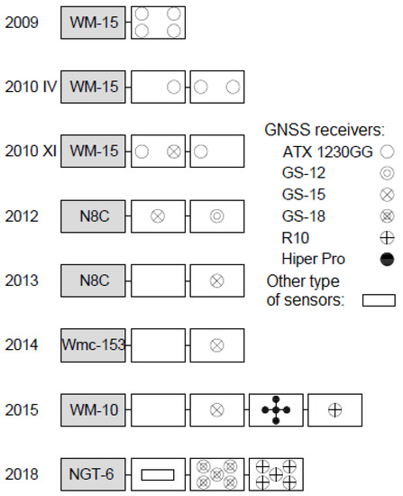
Figure 1.
Scheme of the distribution of GNSS receivers in each measurement campaign.
In this paper, the authors present the results of comparative analysis of the measurements made on the selected test section, characterized by rather unfavorable conditions both for tacheometric and GNSS measurements. The measurements presented and the analysis of their results were made as part of the works carried out in the InnoSatTrack project (BRIK project) [39,40,41].
2. Materials and Methods
2.1. Characteristics of the Test Track
The test section of the track is located on the railway line number 211 (Chojnice-Kościerzyna in northern Poland), between kilometers 9+600 m and kilometer 12+000 m. The selected section of the railway line is a single-track line. According to the technical documentation, the testing ground was the area of the change in the direction of the railroad with the turning angle of 44.112753o. The location plan of the measurement testing ground reproduced on the basis of the satellite map is shown in Figure 2. The pavement of the test track is a ballast structure made in the technology of a continuous welded track. In kilometer 9+600 m up to kilometer 11+200 m, it consists of rails with a profile 49E1 according to European standard EN 13674-1 on prestressed concrete sleepers type PS-94/SB4/1435/49E1 with an SB-4 type fastening system. From kilometer 11+200 m up to kilometer 12+000 m, the 49E1 rails are fixed to sleepers of an old fashion type INBK by a K-type fastening system. The track superstructure is shown in Figure 3 and Figure 4. The whole section of the test track was subject to repair works carried out on section Chojnice - Brusy in 2019. The replacement of the damaged components of pavement (sleepers, ballast) and the adjustment of the track of axis was part of repair works. Due to the fact that there is small railway traffic on this line (2 pairs of passenger trains planned during the day, run by light Diesel Motor Unit SA-109), it was assumed that on the test section, no significant deformations of track geometry will appear. The geometrical characteristics of the test section are shown in Table 1. The track is located in a rural area. The area is only partially GNSS friendly, due to the high forestation near the track.
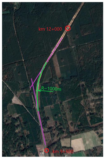
Figure 2.
Location plan of the measurement testing ground.

Figure 3.
Measuring set number 1 to measuring using the GNSS technique.
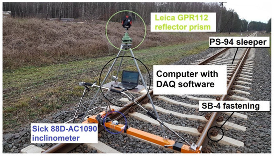
Figure 4.
Measuring set number two for tacheometric measurement.

Table 1.
Geometric layout of the analyzed section of the railway line.
2.2. Apparatus
The primary objective of these measurements was to evaluate the compatibility of the coordinates of the axis of the track obtained with the use of alternative methods of measurement relative to one another, which are the method of mobile satellite measurements, GNSS RTN (Real Time Network) measurements with the use of the ASG Eupos reference network, and tacheometry. ASG-Eupos is a Polish nationwide network of reference stations offering RTN (Real Time Network) corrections. The closest reference station of the ASG Eupos network is located approximately 8 km from the test site. The free position of the tacheometer was bound additionally to the control network points [10,11]. Three measurement sets were prepared.
Set number 1 (Figure 3) for GNSS RTN measurements consisted of:
- Measurement trolley Graw TEC1435 with the tripod; and
- GNSS receiver Trimble R10 operated by a Trimble TSC-3 controller.
Set number 2 (Figure 4) for measuring using spatial indentations consisted of:
- Measurement trolley Graw TEC1435 with the tripod for measuring the clearance;
- Distance meter prism Leica GPR121;
- Inclinometer SICK ACI090-88D together with the control unit; and
- Tacheometer Leica TPS 1201 RTCM.
Both measurement sets made it possible to record the same trajectory of the measurement trolley because the GNSS receiver and the prism were mounted to the same supporting structure. Horizontal coordinates were determined in the PL-2000 system. Suitable vertical offsets resulting from the construction of measuring devices were taken into account in accordance with the specification of the equipment. The tacheometer was set on the positions located along the railway track, the positions of which were determined using the method of resection to four marks of the control network. The maximum length of sight 200 m was assumed.
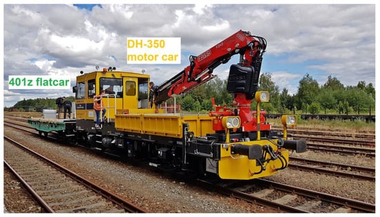
Figure 5.
Measuring set number 3 for making mobile satellite measurements.
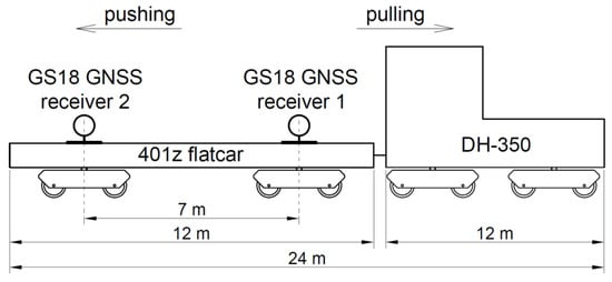
Figure 6.
Configuration of the devices of measuring set number 3 and the directions of running.
- Power car DH-23,300.11;
- 401z flatcar with fitted mounting racks for measurement devices;
- Set 6 of receivers Leica Viva GS18 operated with Leica CS20 controllers;
- Additional GNSS receivers (Leica Viva GS15, Trimble R10, Topcon HiPerHR);
- Inclinometer SICK ACI090-88D together with the control unit; and
- Additional measuring equipment (including Furuno GNSS compass, gyroscopes, accelerometers).
Set number 3 allowed the registration of the trajectory of GNSS receivers. Two of the six receivers Leica Viva GS18 were located over the center plates of the car bogies (1 and 2). Hence, their trajectory in the horizontal plane corresponds to the trajectory of the axis of the railway track. In further analyses, the authors focused on the measurement signal obtained just from these receivers. The receiver marked with number 1 was mounted on car 401z from the side of power car DH-350, the receiver marked with number 2 was on the opposite side of the car 401z. Other receivers were used for testing purposes, for the analysis of the reliability of measurement signal registration. For example, in work [42], the methodology of determining the cant using accelerometry and the trajectory of the measuring vehicle was already proposed.
2.3. Measuring Series
As part of the research discussed, four basic measurement series were performed. They included measurements of GNSS raw data with the registration of a frequency of 1 or 20 Hz and the measurements of coordinates using tacheometry at the interval of 10 m. The data recorded in each measurement series are listed below:
Series 1 from kilometer 12+000 m to kilometer 9+600 m—GNSS measurement session:
- GNSS continuous measurement (raw data registration) with a frequency of 1 Hz;
- Measurement of the track geometric parameters (cant, gauge) by means of the measurement trolley.
Series 2 from kilometer 9+600 m to kilometer 12+000 m—tacheometric measuring session:
- Measurement of prism coordinates every 10 m and at each hectometer post (tacheometric measurement of the section was made from seven free positions, each of which was tied to at least four marks of the control network);
- Measurement of cant by means of the inclinometer.
Series 3 from kilometer 9+600 m up kilometer to 12+000 m—first measurement session of the mobile satellite measurements:
- Continuous GNSS measurement (registration of raw data) with a frequency of 20 Hz, pushing the measurement platform at an average speed of 25 km/h.
Series 4 from kilometer 12+000 m up to kilometer 9+600 m—second measurement session of the mobile satellite measurements:
- GNSS continuous measurement (registration of raw data) with a frequency of 20 Hz, pulling the measurement platform with an average speed of 55 km/h.
2.4. Analysis of the Results of Measurements
2.4.1. Limitations of the Methodology Used
The measurements carried out, as an assumption, were not intended to reproduce the coordinates of the axis of the track in exactly the same points of the route measured. This approach was not taken into account due to the fact that the practical implementation of the measurement methodology with the use of GNSS techniques is based on the registration of data with a specified time interval. At present, standard registration of raw data with a frequency of 20 Hz and RTN positioning in 1 Hz mode (with interpolation up to 20 kHz) provides numerous sets of data, which are then used to estimate the geometric systems of the axis of the track. For this reason, it is not the recorded coordinates that are compared but geometric systems of the axis of the track, which are estimated on their basis.
Considering the problem of interference resulting from the proximity of GNSS receivers [43,44,45], the authors introduced an appropriate control procedure. In the development of GNSS observations, within each measurement epoch, the spatial relationship between the obtained receiver positions is examined. The applied method of data processing, taking into account post-processing of raw satellite data and geodetic alignment of observations, ensures a higher accuracy is obtained. One of the methods of performing calculations by the authors was introduced in [38]. Due to time limitations arising from the use of the railway line, the measurement was made in two directions relative to chainage (back and forth). The coordinates coming from tacheometric measurement were determined according to chainage. In turn, the coordinates obtained from the raw dynamic measurements (that is, kinematics) were determined contrary to chainage. In order to agree on the measurements carried out by using the measurement trolley in opposite directions, a suitable numerical algorithm was developed. As a reference value of measurement, the points measured using the tacheometric method were accepted. To compare the results from various measurement techniques, spatial relations between the recorded coordinates were analyzed without reference to the track axis.
2.4.2. Measurement Offsets
The supporting structure of the mobile set (measurement trolley with tripod) does not provide the centering of the vertical axis of measurement instruments relative to the rails. Therefore, it is not possible to compare directly the measurements made in opposite directions (with respect to chainage). That is why it was first necessary to take into account structural offsets.
The measurement trolley with the measurement system mounted was measured using a tacheometer. Based on the obtained coordinates (spot heights of characteristic points), a geometrical system of the device was developed, and on its basis, the shift of the signal was calculated in relation to the axis of the track. The designated fixed displacement between the axis of the track and the vertical axis of the measuring instrument mounted on the tripod was 0.198 m. The spatial model of the measuring is shown in Figure 7. Figure 8 shows the result of two measuring series performed in both directions with respect to the chainage.
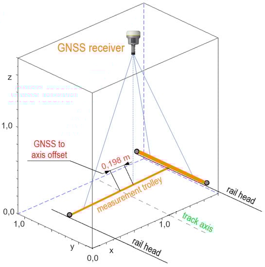
Figure 7.
Spatial model of the measuring set in the local system of xyz coordinates.
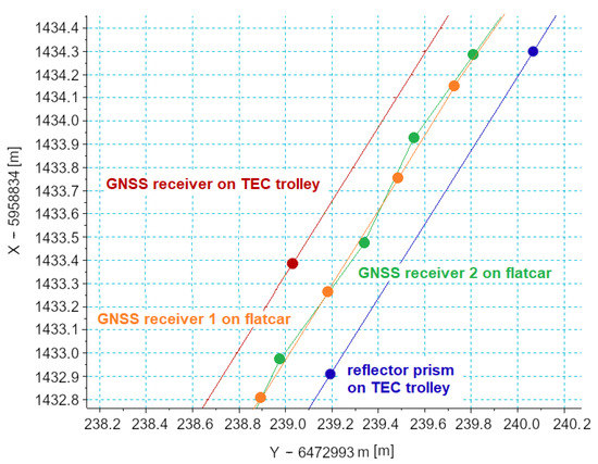
Figure 8.
Points measured using GNSS techniques (kinematics), and tacheometry presented on the grid of the coordinates of PL-2000 system.
Due to the similar elevation (height) of the GNSS receiver and the reflector prism, the influence of the track cant on the lateral shift of the coordinates in relation to each other in subsequent measurement series can be neglected. Additionally, mobile antennas during MSM runs were moving on a similar elevation.
2.4.3. Algorithm of Coordinate Adjustment
The overlap of each point in the plane coincident with the plane of the track was made perpendicularly to the tangent of the measuring signal, designated in the place the measurement was made, with the value of the calculated offset of the construction measurement trolley. Due to the fact that the measurement included sections of the track situated on both straight lines and curves, it was decided to perform a separate shift of each of the measurement points.
For this purpose, an algorithm was developed, in which the function executing a linear mobile regression was implemented. For each of the measurement points (except the first and the last endpoints 5), the auxiliary matrix of coordinate points closest to the surroundings was defined, for which the parameters of linear regression were calculated. This allowed for the determination of the straight line perpendicular (for rolling the measurement) to the tangent in point i.
The gradient of a straight perpendicular line to the tangent calculated by the smallest squares passing through the point is:
where is the gradient of line [-],
In the next step (iteratively), shifting of the set of coordinates is made by a distance resulting from the offset of the axis of the instrument relative to the axis of the track:
where are the horizontal coordinates [m].
Figure 9 shows the schematic diagram for the coordinate adjustments. The algorithm was implemented in the program SciLab 6.1.0. It should also be noted that for the comparative analysis relating to the trajectory of the measuring instrument, taking into account the cant of the track on the curve is not necessary. The recorded data about the tilt angle will be used by the authors for future analyses carried out as part of the BRIK project.
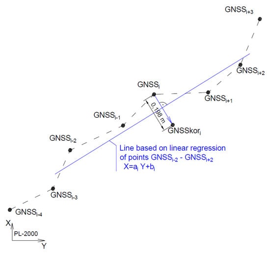
Figure 9.
Schematic diagram of the coordinate adjustments.
2.5. Analysis of the Differences of the Trajectory Recorded in Each Series of Measurement
After the removal of the offsets of measurement series carried out in different directions, the analysis of the positions obtained was performed. Due to the fact that the measurements were performed without time synchronization (at different times) and spatial (locations were near to one another with the accuracy of several centimeters along the axis of the track), the analysis was performed, approximating the position of measurement points measured using the kinematic method GNSS. The absolute difference in the resulting trajectory was called the distance between the coordinate of the point measured using the tacheometric method and the straight line connecting the signals nearest to this point recorded using the GNSS method. A similar method for the determination of errors, although in the measurements of the sea, was presented in [31]. The schematic diagram for calculations is shown in Figure 10.
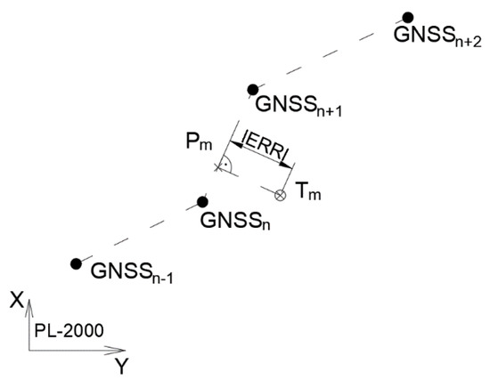
Figure 10.
Schematic diagram of the calculation of horizontal absolute residuals between the results of tacheometric measurement and GNSS.
The algorithm for calculating the residuals can be presented in the following steps:
- Designation of the parameters of the straight line joining adjacent coordinates measured by GNSS:where is the -intercept of the line [m].
- Designation of the parameters of a straight perpendicular line to the straight longitudinal relative to the track axis (4):
- Calculating the coordinates of the projected auxiliary point ; the point measured using tacheometric method was projected onto a straight line between two points measured using GNSS method (GNSSn and GNSSn+1):
- Calculating the error of the relative position of GNSS measurement points relative to the points obtained from tacheometry, as the distance between Tm and Pm points:where is the absolute difference in the resulting trajectory [m].
Calculations made according to the algorithm specified above allow the absolute value of the error to be found regarding designating the position using GNSS techniques in the surroundings of tacheometric measurement.
The distribution of residuals between the points of kinematic measurement GNSS and the geometric system estimated on the basis of tacheometry was also analyzed. For this purpose, the distance of the GNSS signal with respect to straight line connecting points obtained from tacheometry was checked. Figure 11 shows the schematic diagram for the calculation of these differences.
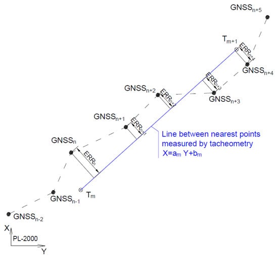
Figure 11.
Relative horizontal errors for all points from GNSS kinematic terms relative to straight lines connecting the positions obtained from tacheometry.
The gradient of a straight line between the closest point measured with the tacheometry – was calculated according to the relationship:
Horizontal coordinates from GNSS measurement and from tacheometry were transformed to appropriate local systems. The axis of the cut-offs of these systems was orientated according to the directions of the straight lines connecting the adjacent points from tacheometry. The beginning of the first system was defined in the first reference point. Then, the individual parts of the signal analyzed in the following local systems were connected to obtain the piecewise signal of the distribution of residuals specified. The schematic diagram for calculating the residuals of a single segment of the measuring GNSS signal located between tacheometric measurements is shown in Figure 12.
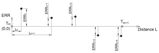
Figure 12.
Schematic diagram of the calculation of the distribution of the residuals: Surveying-kinematics GNSS.
The equation of transformation and matrices of translation and rotation are shown in the following Equation [46]:
where is the distance [m] and is the altitude [m].
The technique accepted to assess the accuracy for determining the coordinates is correct only in case of the measurement of straight-line sections in a horizontal plane. In the case of moving on the straight section, a theoretical axis of the track between two points measured using the tacheometric method will be a straight section, and on the curve, it will be a curved section, so a theoretical versine will appear. Hence, the error of the designation of position can be overestimated or underestimated in some ranges. A diagram showing the influence of versine on the error to reproduce the position is shown in Figure 13.
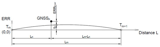
Figure 13.
The influence of the versine on the value of error .
Additional calculations for the curvilinear section were introduced, evaluating the theoretical versine of the curve and taking them into account in further calculations:
where is the curve radius [m] and is the versine [m].
3. Results
The first step of the analyses of results of the measurements was to calculate the residuals between the results obtained in the tacheometric measurement in relation to the measurement of GNSS with the receiver installed on the measurement trolley. For this purpose, the first algorithm was used to assess the residuals for the coordinates of the closest points. A diagram of the residuals calculated in accordance with the method presented is shown in Figure 14. It is clear that in particular ranges related to the successive free station of the tacheometer, the absolute value of error for the designation of the position is at a comparable level.
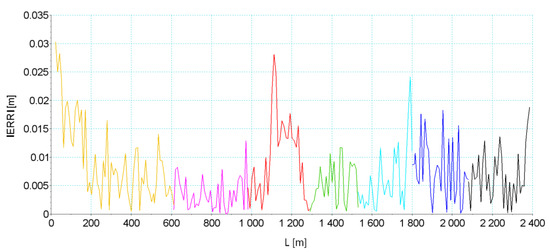
Figure 14.
Signal of the GNSS residuals in relation to the tacheometric surveying; particular colors denote the ranges of respective sections in tacheometric measurement.
In order to assess whether a deviation of the recorded signal is random, or is subject to a constant offset, the analyses were performed using the second algorithm. This algorithm allows assessment of whether the measured coordinates are arranged alternately on both sides of the theoretical straight line designated between the coordinates measured by the tacheometer (case of random error, which means that the coordinates are determined exactly but inaccurately) or whether they are grouped on one side (case of constant error, meaning that the coordinates are designated precisely but inaccurately). The results of the analyses are shown in Figure 15 and Figure 16 and in Table 2. The drawings are divided into the analysis of individual signals and the collective analysis of the signals obtained from all receivers (from the receivers mounted on the TEC trolley and on the flatcar).


Figure 15.
Distribution of errors for different GNSS signals in relation to the tacheometry measurements.
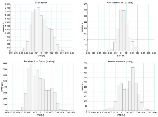
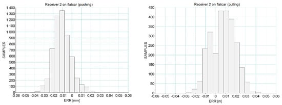
Figure 16.
Histograms of errors for different GNSS signals in relation to the tacheometry measurements.
Table 2.
Mean and σ values calculated from the ERR signal before and after the versine effect correction.
The graphs in Figure 15 show that different receivers recorded signals that can generally be considered qualitatively consistent. However, there are some shifts that indicate the appearance of quasi-systematic errors. Additionally, the signal from the receiver mounted on the TEC trolley in the middle section of the measured tracks showed a distinctly different trend in the error value distribution. It may result from a local decrease in the accuracy of measurements, due to a temporary loss of visibility of some observed satellites. Additionally, the increased measurement uncertainty given by the receiver on the distance between kilometer 10+600 m and 10+700 confirmed this fact.
Figure 16 shows the histograms representing the empirical density distribution of the error value along the length of the test track section. These distributions show that the average offsets for various GNSS measurement methods relative to the reference, which is a tacheometric measurement, amount to several millimeters with a relatively small standard deviation (see Table 2).
As shown in Table 2, in the section between kilometer 10 + 200 m and kilometer 10 + 900 m, there is a circular curve with a radius of about 1000 m. This value is known from the technical documentation of the railway line and it was additionally confirmed in the GNSS signal analysis (curvature estimation based on the measurement).
The algorithm adopted for analysis uses the chord as a reference line. Therefore, the versine of the curve in relation to this chord does not constitute a positioning error and its influence should be eliminated according to the algorithm presented in Section 2.5 (see Figure 13). It should be expected that the distribution of versine relative to the reference line which is the chord between successive points and , will reflect the geometric layout in the form of a sequence of half-waves. The peak values of these versines are expected to be close to the calculated middle versines, which means about 12.5 mm (radius ~1000 m, chord ~10 m).
The arc effect interpreted in this way can be observed in Figure 17, which shows a fragment of the signal along the length of the circular arc. The graph schematically shows a single sequence of versines with respect to one chord between the two reference points (measured with the use of tacheometry). It is worth noting that the values of the relative error in the middle of the chord are the lowest. This can lead to wrong conclusions as the versine in the middle of the chord is expected to be the greatest (as shown in Figure 13). However, it should be remembered that there are constant offsets on the GNSS signal relative to the reference line (measured by tacheometry). The application of the correction for this section resulted in an increase in the error value in relation to the error value before the correction , while this result is simply closer to the real one. This is because the occurrence of theoretical versines affected the error distribution and resulted in an apparent reduction in error. The graph after correction shows a more even distribution of the error value but at a higher level of the mean value.
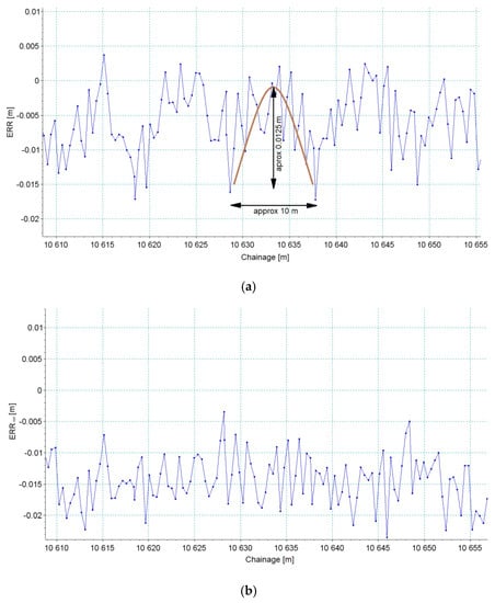
Figure 17.
Signal of the ERR value along the length of a fragment of a railway line in a circular curve with a radius of = 1000 m. (a) Signal before correction of the arc versines, (b) Signal after correction.
Figure 18 shows the entire circular curve segment before and after correction. Visual assessment of the correction is certainly difficult due to the character (scatter plot) of the signals. However, the effect of filtering out certain signal components (versines) in the adopted chord-versine method can be observed.
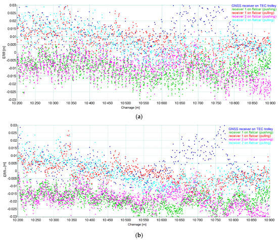
Figure 18.
Signal of the value along the length of the entire circular curve with a radius of = 1000 m. (a) Signal before correction of the arc versines, (b) Signal after correction.
The calculated values of the statistics are presented in Table 2. The values before/after correction should not be interpreted in a sense of improvement or deterioration of the signal quality. Between these values, there is a kind of transition function, the parameters of which are both determinate (radius of the curve, chord length) and random (offset resulting from the vehicle fitting into the track). Therefore, it should be expected that the accuracy characteristics after correction are closer to the real ones. Thus, the increase in the values of sigma is due to the fact that despite the smoothing of the signal, the local error levels changed and hence the signal is more dispersed around the mean value calculated for the entire arc segment. Finally, it could be noticed that the accuracy of the GNSS methods allows the detection of versines for a typical arc radius value like = 1000 m with a relatively short chord of 10 m.
4. Discussion
The resulting empirical distribution of the residuals between the tacheometric measurement and GNSS on the measurement trolley (Figure 15, Table 2) indicates the value of a non-zero relative offset of 5 mm. This value with a standard deviation of 10 mm indicates the presence of a systematic error. From the graph of the residuals on the length of the test track (Figure 14), it can be concluded that this distribution constitutes intervals (positions of tacheometer) that are substantially uniform and have a certain average value. Therefore, the estimated mean value of relative residuals on the part of tacheometry is influenced by such factors as the accuracy of determining the coordinates of the instrument relative to the marks of control networks (5 ÷ 13 mm, depending on the position), the measurement error of the measurement car, and the error of the method of sliding over the coordinates (estimated at the level of individual millimeters, measurement using a high-quality tacheometer 0.5″). Additionally, from the side of satellite measurements, a few millimeters of uncertainty of the reproduction of directions should be expected.
The situation is similar in the case of measurements carried out using MSM technique. Additionally, in this case, fixed relative shifts are clearly visible. These movements are characterized by opposite signs in the case when you travel on the platform in front of the power car (pushing the platform) and the platform behind the power car (pulling the platform). The difference between these values in the case of both GNSS receivers is about 15 mm, which provides a strong suggestion that the shift is the result of a different operation of the car as it travels in two directions. The car is characterized by certain clearances between the side surfaces of the railheads and the rims of the wheels. Therefore, the center plate of the car will not move all the time on the trajectory in accordance with the shape of the axis of the bogie, because they will be pushed into the one or the other rail course. However, there is an especially high risk when a fixed shift when pushing the measuring car, during which an uneven reaction force of the buffers can result in misalignment of the car being pushed. Such a situation is less likely in the case when the car is pulled because the chain coupling is single and placed in the axis of the car. It is expected that an additional source of errors will be in the nosing of the car and the shift of the car structure in relation to the cars. The satellite measurement itself is burdened with millimeter uncertainty for the determination of positions. A photo of the coupling of the car is shown in Figure 19.
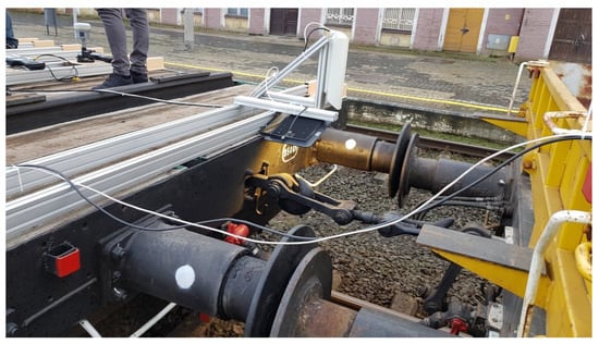
Figure 19.
The coupling connecting the power car with the platform car.
It can also be noted that during MSM measurements for the GNSS receiver positioned further away from the power car, the standard deviation of error was the same as in the case of measurements performed with the use of the measurement trolley with the GNSS receiver mounted. The standard deviation of error increased slightly, with an increase of the speed of the measurement car, and can be due to greater vehicle side motions.
While driving at 50 km/h, two distinct vertices appeared in the histogram, which can be the result of the appearance of an adverse satellite system on the section of chainage 9800–10,100 and a temporary increase of the error in the determination of the GNSS position.
When overlapping the five charts of the residuals onto each other, it is clear that errors are not random, and two trends can be determined:
- From 9600 up to 10,700, a decrease in the value of error;
- From 10,700 up to 11,800, an increase of error.
This can be caused by the increase of errors of the polygonal traverse, where the coordinates of control network marks were determined.
5. Conclusions
Tacheometric measurements have the highest accuracy for determining the coordinates. It can be assumed that the measurement error related to the instrument oscillates within the boundaries of a single millimeter.
The obtained accuracy of measurements with the use of GNSS methods (static and mobile) meets the accuracy requirements for inventory measurements of railroad tracks. The resulting difference values and their standard deviations for the MSM method do not differ qualitatively from the residuals, which were calculated in the GNSSS method; therefore, it is reasonable to conclude that the MSM method provides an efficient alternative to the methods used now.
Continuous kinematic GNSS measurement provides an efficient alternative to tacheometric measurements. It enables measurements with a capacity of more than 4 km/h with the use of the manual method (the measurement truck pushed on the track) or tens of km/h in the version of the mobile method (measuring the vehicle pulling the platform with measuring instruments).
Continuous kinematic GNSS measurement is less accurate in the determination of the single coordinates of points. However, due to the high frequency of data recording, it is possible to obtain a distance between the measurement points of 0.2 ÷ 0.5 m. This enables the use of statistical methods and filtering of the signal obtained in this way, which leads to a reduction of the uncertainty related to the reproduction of the track axis.
Based on the assumptions regarding signal filtration indicated above and the technical capabilities of recording devices (GNSS receivers with controllers), the following MSM measurement speeds are recommended:
- For measuring systems with a data recording frequency of 1–5 Hz, in a man operated trolley, with the speed of the human step (about 3–6 km/h);
- For measuring systems with a data recording frequency of 20 Hz–15–30 km/h; and
- For measuring systems with a data recording frequency of 100 Hz, the possibility to measure up to 180 km/h.
Due to technical constraints, mobile measurements were made at speeds of up to 60 km/h. It should be assumed that as the speed increases, the effect of the wagon’s oscillation relative to the track will increase, so-called hunting oscillation. In order to assess the impact of this phenomenon, a reference measurement should be carried out, for example, measurement using the inertial method or the vision one. The research carried out by the authors showed a low effect of hunting oscillation at speeds below 30 km/h. In subsequent test measurements, the use of 100-Hz GNSS receivers is planned, in order to verify the thesis about the possibility of increasing the measurement speed.
The mean value of residuals at a level of 5 mm obtained in GNSS studies with a standard deviation equal to 10 mm is the result of several factors related to the methods presented (error on marks of the geodetic control network, tacheometry error, measurement error of the trolley and the method of transforming the coordinates, error of GNSS positioning method).
The analysis of the curve section clearly indicates that the random error of determining the position using the MSM method is clearly smaller than the versine of the curve, which gives way for further works related to the analysis of curvilinear sections using GNSS measurements.
Author Contributions
Conceptualization, C.S., A.W., W.K., K.K., J.S. (Jacek Szmagliński), P.C., P.D., S.G.; methodology, A.W., W.K., C.S., J.S. (Jacek Szmagliński), P.C., S.G., P.D., K.K.; software, J.S. (Jacek Szmagliński), P.C.; validation, P.C., J.S. (Jacek Szmagliński); formal analysis, P.C., J.S. (Jacek Szmagliński); investigation, A.W., C.S., W.K., K.K., J.S. (Jacek Szmagliński), J.S. (Jacek Skibicki), P.C., P.D., M.S., R.L., S.J., S.G., K.C.; resources, A.W., C.S., W.K., K.K.; data curation, C.S., P.D., J.S. (Jacek Szmagliński), P.C.; writing—original draft preparation, J.S. (Jacek Szmagliński), P.C.; visualization, J.S. (Jacek Szmagliński), P.C.; supervision, W.K. All authors have read and agreed to the published version of the manuscript.
Funding
Works were carried out as part of the research project “Development of innovative methods for determining the precise trajectory of rail vehicle” InnoSatTrack (POIR.04.01.01-00-0017/17), financed by NCBiR and PKP PLK SA.
Conflicts of Interest
The authors declare no conflict of interest.
References
- Esveld, C. Modern Railway Track; MRT Productions: Zaltbommel, The Netherlands, 2001; pp. 35–53, 107–170. [Google Scholar]
- Kardas-Cinal, E. Selected problems in railway vehicle dynamics related to running safety. Arch. Transp. 2014, 31, 37–45. [Google Scholar] [CrossRef]
- Koc, W.; Chrostowski, P.; Specht, C. Finding Deformation of the Stright Rail Track by GNSS Measurements. Annu. Navig. 2012, 19, 91–104. [Google Scholar] [CrossRef][Green Version]
- Koc, W.; Specht, C.; Chrostowski, P.; Palikowska, K. The accuracy assessment of determining the axis of railway track basing on the satellite surveying. Arch. Transp. 2012, 24, 307–320. [Google Scholar] [CrossRef]
- Beugin, J.; Marais, J. Simulation-Based evaluation of dependability and safety properties of satellite technologies for railway localization. Transp. Res. Part C Emerg. Technol. 2012, 22, 42–57. [Google Scholar] [CrossRef]
- Strach, M.; Uznański, A. Analysis of the implementation of GNSS satellite surveying technology in determining geometry of railways. Rep. Geod. 2011, 1, 439–445. [Google Scholar]
- Lenda, G. Determining the Geometrical Parameters of Exploited Rail Track Using Approximating Spline Functions. Arch. Civ. Eng. 2014, 60, 295–305. [Google Scholar] [CrossRef]
- DB Netz AG. German Railway Standard, 883.2000 DB_REF-Festpunktfeld; DB Netz AG: Frankfurt, Germany, 2016. [Google Scholar]
- DB Netz AG. German Railway Standard, 883.9010 Begriffe und Definitionen, Richtlinie, Version 7.0; DB Netz AG: Frankfurt, Germany, 2018. [Google Scholar]
- PKP Polskie Linie Kolejowe S.A. Polish Railway Standard, Wytyczne dla Osadzania Znaków Regulacji Osi Toru na Konstrukcjach Wsporczych (Słupach) Sieci Trakcyjnej Ig-6; PKP Polskie Linie Kolejowe S.A.: Warsaw, Poland, 2011. [Google Scholar]
- PKP Polskie Linie Kolejowe S.A. Polish Railway Standard, Standard Techniczny Określający Zasady i Dokładności Pomiarów Geodezyjnych dla Zakładania Wielofunkcyjnych Znaków Regulacji Osi Toru Ig-7; PKP Polskie Linie Kolejowe S.A.: Warsaw, Poland, 2012. [Google Scholar]
- State of NSW. Australian Railway Standard, Standard Railway Surveying THRTR13000ST; State of NSW: Sydney, Australia, 2016. [Google Scholar]
- Meinck, M. Die neue Vermessungsrichtlinie Ril 883.2000 DB_REF-Festpunktfeld. In Proceedings of the Seminar Gleisbau 2017—Planung und Vermessung, Berlin, Germany, 3–4 March 2017. [Google Scholar]
- Izvoltova, J.; Villim, A.; Kozák, P. Determination of Geometrical Track Position by Robotic Total Station. Procedia Eng. 2014, 91, 322–327. [Google Scholar] [CrossRef]
- Bitterer, L.; Hodas, S. Geodetic Surveying of Railway Objects. WIT Trans. Built Environ. 1998, 34, 3–12. [Google Scholar] [CrossRef]
- Network Rail. British Railway Standard, NR/L2/TRK/3201_Network Rail—Management of Tight Clearances and Track Position; Network Rail: London, UK, 2010. [Google Scholar]
- Network Rail. British Railway Standard, NR/L3/TRK/0030 NR_Reinstatement of Absolute Track Geometry (WCRL Routes); Network Rail: London, UK, 2008. [Google Scholar]
- Polskie Linie Kolejowe, S.A. Polish Railway Standards, Standard Techniczny O Organizacji i Wykonywaniu Pomiarów w Geodezji Kolejowej GK-1; PKP Polskie Linie Kolejowe S.A.: Warsaw, Poland, 2015. [Google Scholar]
- Glaus, R. The Swiss Trolley—A Modular System for Track Surveying; Schweizerischen Geodatischen Kommission: Zurich, Switzerland, 2006. [Google Scholar]
- Specht, M.; Szmagliński, J.; Specht, C.; Koc, W.; Wilk, A.; Czaplewski, K.; Karwowski, K.; Dąbrowski, P.S.; Chrostowski, P.; Grulkowski, S. Analysis of Positioning Methods Using Global Navigation Satellite Systems (GNSS) in Polish State Railways (PKP). Sci. J. Marit. Univ. Szczec. 2020, 62, 26–35. [Google Scholar] [CrossRef]
- Spinsante, S.; Stallo, C. Hybridized-GNSS Approaches to Train Positioning: Challenges and Open Issues on Uncertainty. Sensors 2020, 20, 1885. [Google Scholar] [CrossRef]
- Specht, C.; Nowak, A.; Koc, W.; Jurkowska, A. Application of the Polish Active Geodetic Network for Railway Track Determination. In Transport Systems and Processes Marine Navigation and Safety of Sea Transportation; Weintrit, A., Neumann, T., Eds.; CRC Press: Boca Raton, IL, USA, 2011; pp. 77–82. [Google Scholar]
- Jiao, G.; Song, S.; Ge, Y.; Su, K.; Liu, Y. Assessment of BeiDou-3 and Multi-GNSS Precise Point Positioning Performance. Sensors 2019, 19, 2496. [Google Scholar] [CrossRef] [PubMed]
- Zhou, F.; Li, X.; Li, W.; Chen, W.; Dong, D.; Wickert, J.; Schuh, H. The Impact of Estimating High-Resolution Tropospheric Gradients on Multi-GNSS Precise Positioning. Sensors 2017, 17, 756. [Google Scholar] [CrossRef] [PubMed]
- Fu, W.; Huang, G.; Yang, Y.; Zhang, Q.; Cui, B.; Ge, M.; Schuh, H. Multi-GNSS Combined Precise Point Positioning Using Additional Observations with Opposite Weight for Real-Time Quality Control. Remote Sens. 2019, 11, 311. [Google Scholar] [CrossRef]
- Ruwisch, F.; Jain, A.; Schön, S. Characterisation of GNSS Carrier Phase Data on a Moving Zero-Baseline in Urban and Aerial Navigation. Sensors 2020, 20, 4046. [Google Scholar] [CrossRef]
- Marais, J.; Berbineau, M.; Heddebaut, M. Land Mobile GNSS Availability and Multipath Evaluation Tool. IEEE Trans. Veh. Technol. 2005, 54, 1697–1704. [Google Scholar] [CrossRef]
- Koc, W.; Specht, C. Selected Problems of Determining the Course of Railway Routes by Use of GPS Network Solution. Arch. Transp. 2011, 23, 303–320. [Google Scholar] [CrossRef]
- Shankar, S.; Roth, M.; Schubert, L.A.; Verstegen, J.A. Automatic Mapping of Center Line of Railway Tracks using Global Navigation Satellite System, Inertial Measurement Unit and Laser Scanner. Remote Sens. 2020, 12, 411. [Google Scholar] [CrossRef]
- Akpinar, B.; Gülal, E. Multisensor Railway Track Geometry Surveying System. IEEE Trans. Instrum. Meas. 2011, 61, 190–197. [Google Scholar] [CrossRef]
- Chen, X.; Landau, H.; Vollath, U. New Tools for Network RTK Integrity Monitoring. In Proceedings of the 6th International Technical Meeting of the Satellite Division of the Institute of Navigation, Portland, OR, USA, 9–12 September 2003. [Google Scholar]
- Yoshimura, A.; Naganuma, Y. A new method to reconstruct the track geometry from versine data measured in the curved track using the Monte Carlo Particle Filter. In Proceedings of the Railway Engineering—2013—12th International Conference and Exhibition, London, UK, 10–11 July 2013. [Google Scholar]
- Koc, W.; Chrostowski, P. Computer-Aided Design of Railroad Horizontal Arc Areas in Adapting to Satellite Measurements. J. Transp. Eng. 2014, 140, 04013017. [Google Scholar] [CrossRef]
- Specht, C.; Koc, W.; Chrostowski, P.; Szmaglinski, J. Accuracy Assessment of Mobile Satellite Measurements Relation to the Geometrical Layout of Rail Tracks. Metrol. Meas. Syst. 2019, 26, 309–321. [Google Scholar] [CrossRef]
- Specht, C.; Koc, W.; Chrostowski, P.; Szmagliński, J. The Analysis of Tram Tracks Geometric Layout Based on Mobile Satellite Measurements. Urb. Rail Transit 2017, 3, 214–226. [Google Scholar] [CrossRef][Green Version]
- Szwilski, T.B. Determining rail track movement trajectories and alignment using HADGPS. In Proceedings of the AREMA Conference, Chicago, IL, USA, 9–12 September 2003. [Google Scholar]
- Specht, C.; Koc, W. Mobile Satellite Measurements in Designing and Exploitation of Rail Roads. Transp. Res. Procedia 2016, 14, 625–634. [Google Scholar] [CrossRef][Green Version]
- Czaplewski, K.; Specht, C.; Dąbrowski, P.; Specht, M.; Wiśniewski, Z.; Koc, W.; Wilk, A.; Karwowski, K.; Chrostowski, P.; Szmaglinski, J. Use of a Least Squares with Conditional Equations Method in Positioning a Tramway Track in the Gdansk Agglomeration. Trans. Nav. Int. J. Mar. Navig. Saf. Sea Transp. 2019, 13, 895–900. [Google Scholar] [CrossRef]
- Dąbrowski, P.; Specht, C.; Felski, A.; Koc, W.; Wilk, A.; Czaplewski, K.; Karwowski, K.; Jaskólski, K.; Specht, M.; Chrostowski, P.; et al. The Accuracy of a Marine Satellite Compass under Terrestrial Urban Conditions. J. Mar. Sci. Eng. 2020, 8, 18. [Google Scholar] [CrossRef]
- Dąbrowski, P.; Specht, C.; Koc, W.; Wilk, A.; Czaplewski, K.; Karwowski, K.; Specht, M.; Chrostowski, P.; Szmagliński, J.; Grulkowski, S. Installation of GNSS receivers on a mobile railway platform—Methodology and measurement aspects. Sci. J. Mar. Univ. Szczec. 2019, 60, 18–26. [Google Scholar] [CrossRef]
- Specht, M.; Specht, C.; Wilk, A.; Koc, W.; Smolarek, L.; Czaplewski, K.; Karwowski, K.; Dabrowski, P.; Skibicki, J.; Chrostowski, P.; et al. Testing the Positioning Accuracy of GNSS Solutions during the Tramway Track Mobile Satellite Measurements in Diverse Urban Signal Reception Conditions. Energies 2020, 13, 3646. [Google Scholar] [CrossRef]
- Koc, W.; Specht, C.; Szmagliński, J.; Chrostowski, P. A Method for Determination and Compensation of a Cant Influence in a Track Centerline Identification Using GNSS Methods and Inertial Measurement. Appl. Sci. 2019, 9, 4347. [Google Scholar] [CrossRef]
- Jang, J.; Paonni, M.; Eissfeller, B. CW Interference Effects on Tracking Performance of GNSS Receivers. IEEE Trans. Aerosp. Electron. Syst. 2012, 48, 243–258. [Google Scholar] [CrossRef]
- Savasta, S.; Rao, M.; Presti, L.L. Interference Mitigation in GNSS Receivers by a Time-Frequency Approach. IEEE Trans. Aerosp. Electron. Syst. 2013, 49, 415–438. [Google Scholar] [CrossRef]
- Gao, G.X.; Sgammini, M.; Lu, M.; Kubo, N. Protecting GNSS Receivers from Jamming and Interference. Proc. IEEE 2016, 104, 1327–1338. [Google Scholar] [CrossRef]
- Schneider, P.J.; Eberly, D.H. Geometric Tools for Computer Graphics; Morgan Kaufmann Publishers: San Francisco, CA, USA, 2003. [Google Scholar]
© 2020 by the authors. Licensee MDPI, Basel, Switzerland. This article is an open access article distributed under the terms and conditions of the Creative Commons Attribution (CC BY) license (http://creativecommons.org/licenses/by/4.0/).