Article

Multi-Temporal Sentinel-2 Data in Classification of Mountain Vegetation

by
Martyna Wakulińska
and
Adriana Marcinkowska-Ochtyra
*
Department of Geoinformatics, Cartography and Remote Sensing, Chair of Geomatics and Information Systems, Faculty of Geography and Regional Studies, University of Warsaw, 00-927 Warsaw, Poland
*
Author to whom correspondence should be addressed.
Remote Sens. 2020, 12(17), 2696; https://doi.org/10.3390/rs12172696
Submission received: 30 June 2020 / Revised: 18 August 2020 / Accepted: 19 August 2020 / Published: 20 August 2020

Abstract

:
The electromagnetic spectrum registered via satellite remote sensing methods became a popular data source that can enrich traditional methods of vegetation monitoring. The European Space Agency Sentinel-2 mission, thanks to its spatial (10–20 m) and spectral resolution (12 spectral bands registered in visible-, near-, and mid-infrared spectrum) and primarily its short revisit time (5 days), helps to provide reliable and accurate material for the identification of mountain vegetation. Using the support vector machines (SVM) algorithm and reference data (botanical map of non-forest vegetation, field survey data, and high spatial resolution images) it was possible to classify eight vegetation types of Giant Mountains: bogs and fens, deciduous shrub vegetation, forests, grasslands, heathlands, subalpine tall forbs, subalpine dwarf pine scrubs, and rock and scree vegetation. Additional variables such as principal component analysis (PCA) bands and selected vegetation indices were included in the best classified dataset. The results of the iterative classification, repeated 100 times, were assessed as approximately 80% median overall accuracy (OA) based on multi-temporal datasets composed of images acquired through the vegetation growing season (from late spring to early autumn 2018), better than using a single-date scene (70%–72% OA). Additional variables did not significantly improve the results, showing the importance of spectral and temporal information themselves. Our study confirms the possibility of fully available data for the identification of mountain vegetation for management purposes and protection within national parks.

Graphical Abstract

1. Introduction

Mountain vegetation is particularly vulnerable to climate change, where the changes of the tree line and plant floor borders become visible [1]. The occurrence of species from various geographical regions in a relatively small area, often being glacial relics, endemics, or endangered species, makes their identification and monitoring extremely important for preserving natural wealth [2]. To achieve this, it is important to provide up-to-date vegetation maps of mountain protected areas.
Despite its high precision, field mapping requires a lot of time and work. In the case of high-mountain vegetation, the limited availability and shorter vegetation period compared to lowlands significantly affect the possibilities of field research. Due to rapid technological progress, remote sensing data, characterized by both greater objectivity and spatial coverage, are increasingly used [3]. The electromagnetic spectrum registered by remote sensing instruments, which create unique spectral characteristics of the analyzed objects, can support traditional methods of vegetation mapping by the use of image classification [3].
Recently, non-parametric classifiers are increasingly employed in vegetation classification [4,5,6,7,8] because of their more flexible approach to training data use than in parametric classifiers, e.g., maximum likelihood (ML) [7,9]. In mountain areas that are difficult to explore, limited training samples and/or imbalanced reference datasets are often available [10]. It was shown that support vector machines (SVMs) [11] are capable of handling small or reduced datasets [9,12,13], which makes SVMs a good fit for studying difficult-to-explore areas that often provided limited data. SVMs also perform well with a large number of classes [9,14,15] and, in comparison to other classifiers, work better with imbalanced data [16,17]. Comparative studies proved that SVMs allowed for achieving higher accuracies than neural nets (NNs) [7] or random forest (RF) [18] in a complex mountain vegetation classification based on different types of remote sensing data.
Mountain vegetation, particularly non-forest, is often rich in species of various physiognomy; as such, in remote sensing research, data resolution is important. The vast majority of works describing the classification of mountain vegetation are based on the use of hyperspectral data [15,19,20,21]. Many studies focusing both on (1) the classification of mountain plant communities [9,20] and (2) specific species [22], identified a large number of classes which, in the context of high spectral resolution, allowed researchers to obtain an overall accuracy (OA) of at least 70%. Another important aspect is to choose the proper unit for classification. The pixel size should allow researchers to determine the appropriate training data set. This is one of the reasons why multispectral data are preferably not classified at a higher level of detail than vegetation type, i.e., combinations of communities [23]. Grouping communities into lower-order units, such as vegetation types, requires expert knowledge because this decision directly affects the number of classes analyzed. To be distinguishable by a sensor, it must be characterized by relatively high spectral diversity [24]. Simplification of the legend often increases the quality and reliability of the results obtained, because it eliminates those classes not identifiable by a given sensor [25]; therefore, the quantitative generalization of the legend is particularly important for a spatial resolution similar to Landsat-8 or Sentinel-2 satellite data. By reducing 15 mountain vegetation categories to 8 classes, the authors improved the Landsat-8 image classification from less than 49% to 66% OA [26]. Similarly, in the case of Sentinel-2 data, the selection of 8 out of 11 classes allowed for a higher OA (from 58% for the detailed legend to 71% for the generalized legend) [7].
Recently, satellite sensors deserve special attention, because the high temporal resolution allows researchers to significantly reduce the costs of constant monitoring of landscape components. Sentinel-2 data can be considered groundbreaking in this context, because in addition to the short revisit time (five days), it is an optimal combination of spectral and spatial resolution. The high frequency of data collection enables the generation of multi-temporal compositions, i.e., images composed of information obtained at different periods of the growing season, which, due to the physiognomic changes occurring in the vegetation, can have a measurable impact on the classification results. Recently published studies on the classification of various vegetation categories based on Sentinel-2 data temporal compositions allow researchers to state that these changes are noticeable and significant (OA equal to 67% for a single date and 78% for 12-images multi-temporal composition [27]; 80.5% for a single date and 88.2% for multi-temporal composition consisting of four images [28]; 87% for a single date to 92% using five images [29]). Although these studies have analyzed forests [28,29,30,31,32], grassy and woody species [33], or floodplain grasslands [27], the study of high mountain vegetation types classification based on multi-temporal Sentinel-2 data are still missing.
Data from different parts of the electromagnetic spectrum can be combined into transformations or vegetation indices that can increase the information capacity added as new bands in classification [34]. To extract uncorrelated information, possibly differentiating the analyzed classes, spectral dimension transformation, e.g., either principal component analysis (PCA) [35] or tasseled cap (TC) [36], is used [6,18]. In optical data analysis, normalized difference vegetation index (NDVI) [37] is commonly used for estimation photosynthetic activity and vegetation greenness, and as such, it is widely applied for the identification and analysis of mapped vegetation units [34,38]. Some authors added more indices, depending on the spectral resolution of the data used to further assess which of them has the greatest impact on the result [39,40]. Comparing the classification accuracies of the datasets with and without added spectral indices, some authors yielded a higher accuracy obtained with these variables [30,40], but some authors also yielded a lower accuracy [6,41]. In mountain and upland areas, the use of digital terrain model (DTM) derivatives seems reasonable; however, predominantly using optical data requires an additional data source, like from airborne laser scanning (ALS) [42] or radar missions [31,43,44]. When using big datasets consisting of multiple scenes or/and additional bands, variable importance analysis is useful to select the best features affecting the accuracy, which was presented by many authors [29,30].
The main aim of this study was to assess the potential of Sentinel-2 multi-temporal data for vegetation types classification in the mountain ecosystem. Our assumption was to fully exploit plant phenology differences, allowing us to separate vegetation types between them, and as such, the multi-temporal classification approach was applied. Previous studies of the parts of this area employed different remote sensing images for vegetation classification [7,15,18,45,46]; however, no combined multi-temporal dataset was used for this purpose. In the context of the sensitivity of mountain ecosystems to climate and other changes, this approach seems to be particularly important, taking into account the variability of vegetation within the growing season, which may not be captured on a single image. We compared single-date and multi-temporal Sentinel-2 data, as well as the best combination of dates with calculated PCA bands and with vegetation indices to select the most optimal dataset. Based on reference polygons and prepared datasets, we performed iterative classification using the SVM algorithm and we assessed the obtained accuracies.

2. Materials and Methods

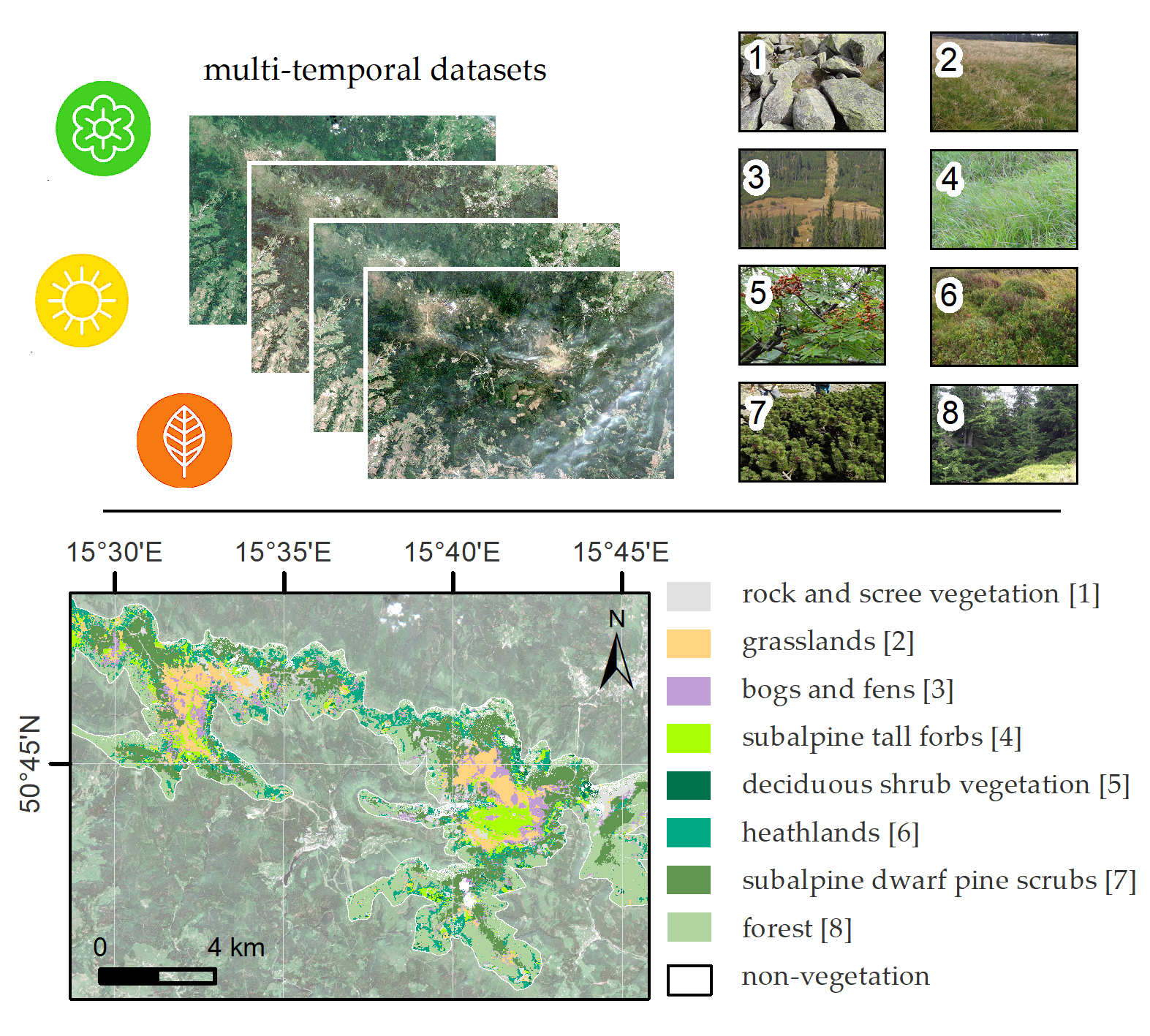
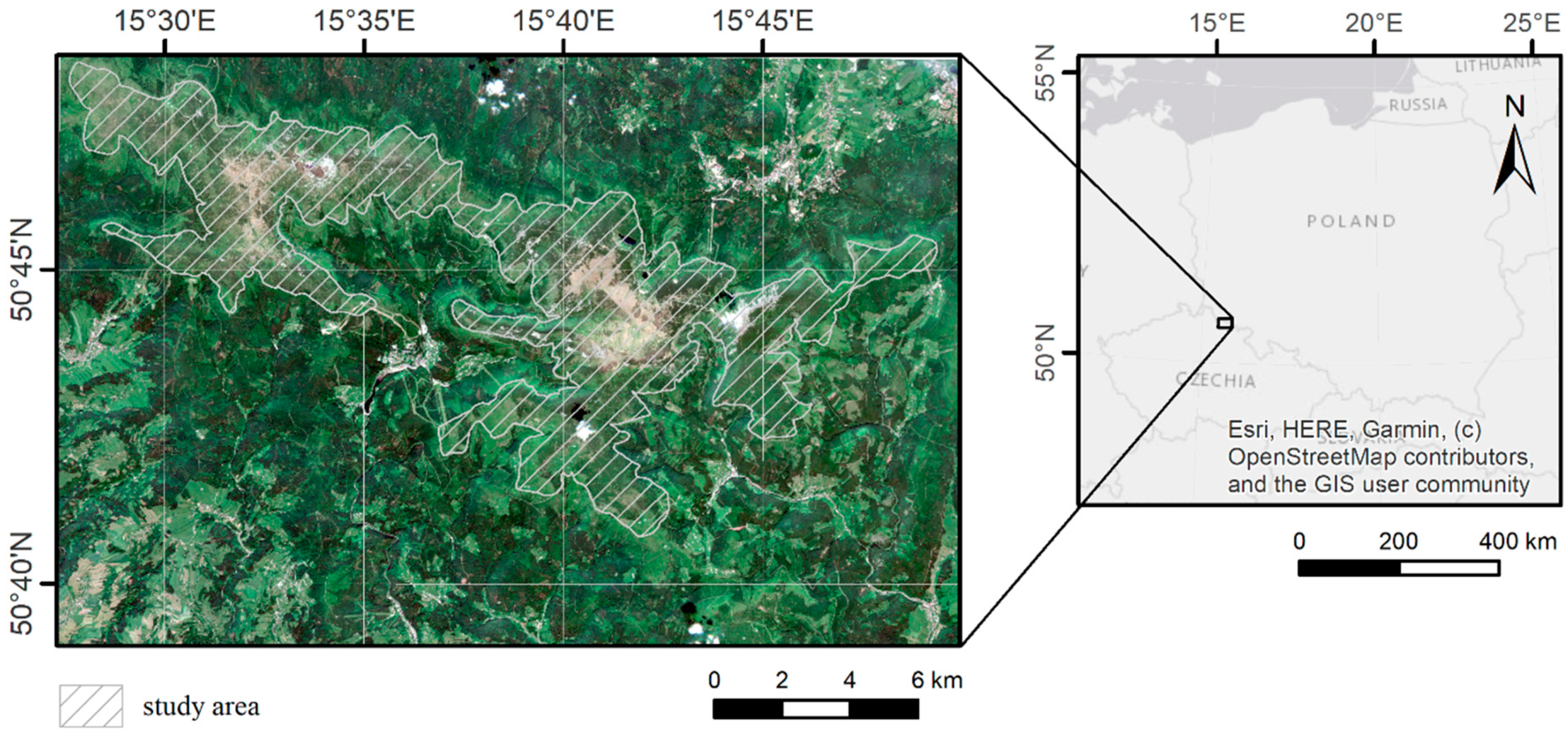
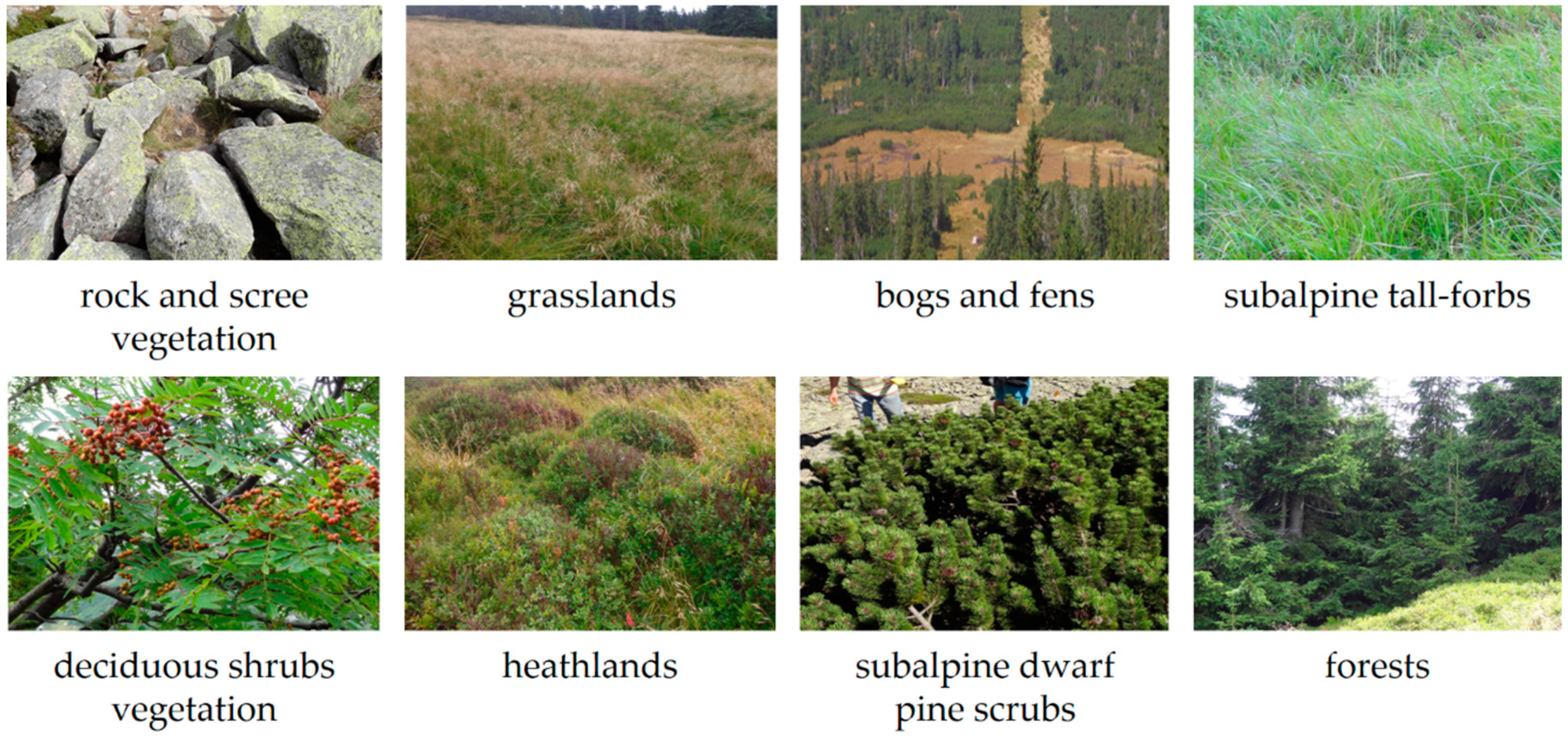
2.1. Study Area and Object of the Study

The study area, covering the highest parts of the Giant Mountains, was located at the Polish–Czech border, within the Krkonoše National Park and Krkonošský Národní Park, respectively; see Figure 1. There were five distinguished plant floors: foothills (up to 500 m above sea level a.s.l), lower (500–100 m a.s.l.) and upper montane zone (1000–1250 m a.s.l), subalpine (1250–1450 m a.s.l.), and alpine zone (above 1450 m a.s.l.). High mountain vegetation was the subject of our analysis (Figure 2), including the one located above the tree line, i.e., the areas located over 1250 m a.s.l. which were considered arctic-alpine tundra [7,47].
The largest areas of the entire Giant Mountains were covered by a mosaic of dwarf pine and grasslands (1500 ha on the Polish side and 3200 ha on the Czech side), playing an important ecological role by protecting the lower forests from snow avalanches [47]. Dwarf pine thickets were dominated by Pinus mugo species. Between their patches, there were shrub communities, consisting of bilberry with a dominance of Calluna vulgaris, Vaccinium myrtillus, and co-occurring Calamagrostis villosa and Deschampsia flexuosa grasses. Within the postglacial cirques, very rich subalpine deciduous shrubs were developed, where there was a regional scale unique community of endemic Salix lapponum willow complex [48]. Bottoms of cirques with fertile soils were covered by herbs from Adenostyles alliariae and Athyrietum distentifoli alliances. The significantly angled slopes above the valleys and postglacial cirques were dominated by species-rich grasslands, where the most popular were Calamagrostis villosa species. A unique feature of the Giant Mountains landscape were the subalpine–subarctic mountain peat bogs. The transition between subalpine and alpine zones was largely dominated by floristically poor communities of grasslands with the domination of Nardus stricta. In the alpine zone, the mountain grasslands are dominated by Juncus trifidus species. Rocks and screes in the upper parts of the Giant Mountains were an excellent habitat for species-rich vegetation and epilytic lichens from Umbilicarion and Rhizocarpion alliances.
Both sides of the Giant Mountains were affected by various factors, including agricultural activities, such as past deforestation and grazing, tourism once the parkland was classified as a protected national park, and sporadic avalanches and debris flows [7,15]. Additionally, in the 1980s and 1990s, an ecological disaster occurred due to strong winds and air pollution [49]. Other vegetation disturbances were caused by pests. The dynamic of vegetation changes were also noted due to expansive species like Molinia caerulea or Calamagrostis villosa encroachment and spreading [50]. All of these factors require a constant need to monitor the vegetation of this valuable mountain area.

2.2. Sentinel-2 Satellite Data

Satellite images with no/minimal cloud coverage from 31 May, 7 and 27 August, and 18 September 2018 were downloaded from the Copernicus Open Access Hub browser. As mountain vegetation physiognomy is variable throughout the growing season (i.e., in late summer/early autumn, alpine and subalpine grasslands begin to discolor, making them easier to distinguish from, e.g., subalpine tall forbs), our assumption was to select data from different phenological phases to capture the vegetative phase, blooming, and senescence of the plants; this data can be reliably collected via the high temporal resolution of Sentinel-2 sensor. However, because study area was located in the mountains, the cloud cover was a significant limitation, which made it impossible to include a given image in the analyses; as such, all available images from the period from March to November, where clouds did not cover more than 10% were taken into account—June and July images were not included, because there were no images available that matched the criteria.
The data with 2A processing level were selected, and the quality of atmospheric correction was assessed by the use of 9 field-collected spectra for radiometrically stable areas (asphalt and concrete). Based on the root mean square error (RMSE), we calculated a consistency of 6.5% for the satellite data. Reflectance 20 m bands were resampled to 10 m in SNAP (ESA Sentinel Application Platform v2.0.2, http://step.esa.int, Brockmann Consult, Skywatch, Sensar, and C-S). To avoid errors caused by the absorption by water, the three 60 m atmospheric bands 1 (coastal aerosol), 9 (water vapor), and 10 (Cirrus) were excluded from the analysis, leaving the bands most commonly used in land applications [6,29,30,31].

2.2.1. Additional Variables Calculation

To improve the method, we decided to use only variables calculated based on one data type (Sentinel-2 images). Our assumption was to add these variables separately to the multi-temporal dataset with the highest accuracy, to check whether these variables improve the accuracy (see Section 2.2.2). The first type of variables were the PCA bands derived from a statistical method of linear data transformation, which determines the new main axis of the coordinate system along with the largest possible data variance by projecting variable values in a multidimensional space [35]. New, uncorrelated variables called principal components were then calculated using the ENVI 5.3 software (Harris Geospatial Solutions, Broomfield, CO, USA). Based on the correlation table of variables that make up the best dataset and then on eigenvalues, the first PCA bands were selected as the most informative. The second type of variables were commonly used vegetation indices that determine the condition of vegetation or canopy water content [52]. Based on availability and the literature, we selected 18 vegetation indices from the spectral resolution of Sentinel-2 data and calculated them using ENVI software (the list of indices presents Table A1 in Appendix A).

2.2.2. Multi-Temporal Datasets Creation

To investigate the effect of combining data from different growing seasons on the obtained accuracies, we stacked the images from four dates and additional variables into 13 combinations (Table 1). We tested each image separately (datasets 1–4) and combined them using two, three, and four different dates (datasets 5–15). Additionally, for the best result, we added calculated vegetation indices and PCA bands (datasets 16–17).
Due to clouds and topographical shadows on individual images, a mask was needed that would allow for the correct interpretation of the result on the final map. The cloud and shadow mask was created based on spectral values from 2 (blue) and 8 (NIR) bands, respectively, and the water vapor map (WVM) product was used in the mask development process as one of the auxiliary materials. The spectral similarity of deep shadows and water surfaces resulted in lakes also being masked. Additionally, the mask defining the range of the study, corresponding to areas above 1250 m a.s.l., was created based on a digital terrain model with a spatial resolution of 1 m derived from georeferenced point cloud from ALS data, filtered and classified in LAStools software (Rapidlasso, GmbH, Gilching, Germany). All masks were developed and applied to the images in ENVI 5.3 software (Harris Geospatial Solutions, Broomfield, CO, USA) using the Build Mask and Apply Mask functions.

2.3. Reference Data

On-ground vegetation type polygons were acquired using GPS Trimble GeoXT receiver (Trimble Inc., Sunnyvale, CA, USA) from 20–30 August 2013 and 30–31 August 2014 field campaigns in the Polish part of the Giant Mountains. As a reference legend, we used the botanical non-forest vegetation map created by Wojtuń and Żołnierz [47], which contains two levels of vegetation organization—communities and types. It was important to check the consistency between the remote sensing and reference data. We decided to use a vegetation type unit because some of the vegetation communities took up very small patches (e.g., 9 m2), which would make it impossible to correctly designate them as training data on the Sentinel-2 pixel. Groups of vegetation types forming communities were more representative in this context. To fit the spatial size of Sentinel-2 data, we sampled field polygons registered in Projected Coordinate System Universal Transverse Mercator_(UTM, zone_33N) in patches equal to or greater than 20 × 20 m per vegetation type, based on the satellite data grid. We also updated on-ground information by checking the consistency between high-resolution Airborne Prism EXperiment (APEX) image (3.12 m, used bands: 640, 547, and 471 nm) from 2012 and PlanetScope image (3 m, used bands: 590–670, 500–590, and 455–515 nm) from 2018, both acquired in September. The visual analysis allowed us to conclude that there were no changes in the polygons within the study area, which, with the adopted 10 m resolution, could indicate that resources are outdated. Based on them, homogeneous patches were identified visually and translated into polygons representing vegetation types (Table 2).

2.4. Classification with Iterative Accuracy Assessment

All stacked datasets were classified using the SVM algorithm with the ‘e1071‘ package [53] of R software [54]. We employed this algorithm due to the non-parametric character allowing for flexibility of training data used, high classification accuracy, and limited classification errors confirmed by many authors [9,12,13,15]. The most commonly used are linear and radial kernel functions, expressed as, respectively [55]:
K ( x i x j ) = x i T x j ,
K ( x i x j ) = exp ( γ x i x j ) 2 ,
where x i x j are the feature vectors, and γ is the gamma parameter.
To select the best SVM parameters, including kernel function, γ, and cost of the penalty (C), tuning of parameters was performed using the ‘tune.svm’ function [53].
To ensure the contribution of each observation in the classification, we decided to use a 100-times iterative procedure of classification and validation of the results following Ghosh et al. [56]. We split the reference polygons into 60:40 for training and validation using a stratified random sampling approach, which allowed us to assess the variability within classes.
Quantitative assessment was based on an error matrix with the OA, as well as producer (PA), user (UA) [57], and F1 [58] accuracies for individual classes. After performing 100 repetitions of classification, the median of each measure was calculated for all datasets, and the distribution of results was presented as a boxplot. The resulting map was developed based on a dominant value calculated from 100 iterations of the best classified dataset.
Additionally, to assess the importance of individual bands from corresponding terms of data acquisition, from the entire ABCD dataset, we calculated variable importance using a receiver operating characteristics (ROC) curve analysis conducted for each vegetation type class using the “caret” package [59], which was based on an SVM model and integrated bootstrapping was repeated 100 times—this was the same procedure we performed for the best dataset with added vegetation indices and PCA bands. The results of these analyses, limited to the 20 most important variables from each dataset, can be seen in Figure A2, Figure A3 and Figure A4 in Appendix A.

3. Results

3.1. Selection of the best Parameters and Dataset

The automatic manipulation of algorithm parameters provided the best configuration possible. Table 3 presents the accuracies obtained for four single-date scenes using default and optimized parameters of the SVM. Table 3 shows that the highest OA was achieved when the radial function was applied. The rest of the datasets proceeded using only optimized parameters, increasing the efficiency of the classification process.
The classification of vegetation types was successfully derived from the Sentinel-2 time series, which, as mentioned prior, was better than using single-date data (Figure 3). The OA of the classification for each of the multi-temporal datasets, obtained from the 100-times iterative procedure of accuracy assessment, was at least two p.p. (percentage points) higher than the results obtained for single-date datasets and ranged from 76.3% to 79.5%. The highest accuracy was achieved for the ABC dataset (the confidence interval (95%) for the classification was (0.7789, 0.8098)). Based on this, PCA bands and vegetation indices were included in this dataset. The correlation table of variables calculated for PCA bands selection showed the lowest correlations (less than 0.35) observed for bands 5, 6, 7, and 8 from A; 6, 7, and 8 from B; and 6, 7, and 8 from dataset C (Table A2 in the Appendix A). The analysis of the eigenvalues allowed for the selection of the first 10 bands of PCA transformation to be the most informative for further processing, as they contained 99.4% of the total variance (Figure A1 in Appendix A); as such, two combinations with additional variables consisted of 40 bands (30 spectral bands + 10 PCA bands) and 84 bands (30 spectral bands + 18 indices calculated for the images acquired on three dates). The combinations comprised of PCA bands and vegetation indices resulted in a lower OA: 77.1% and 79.2%, respectively (Figure 3).

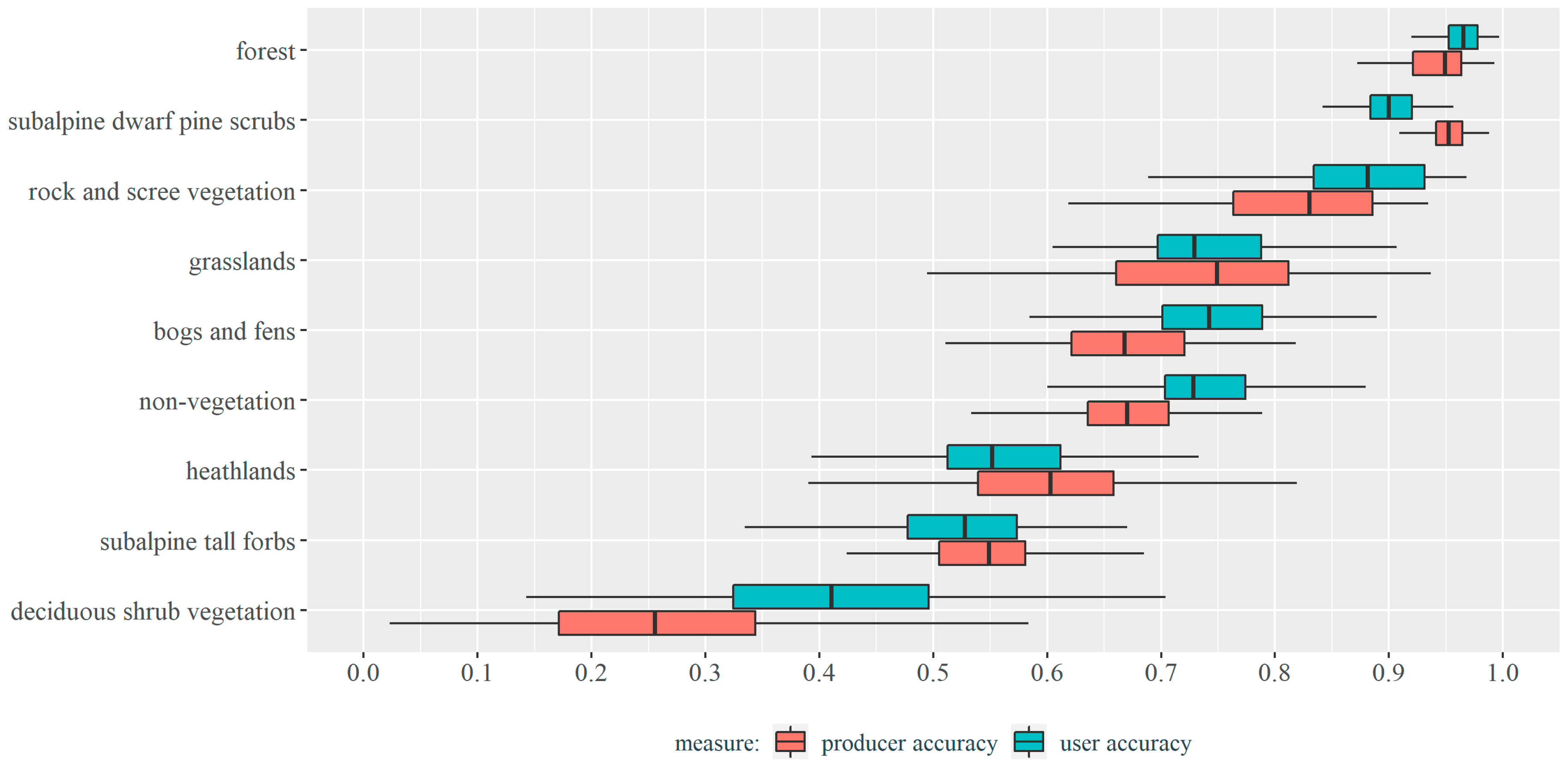
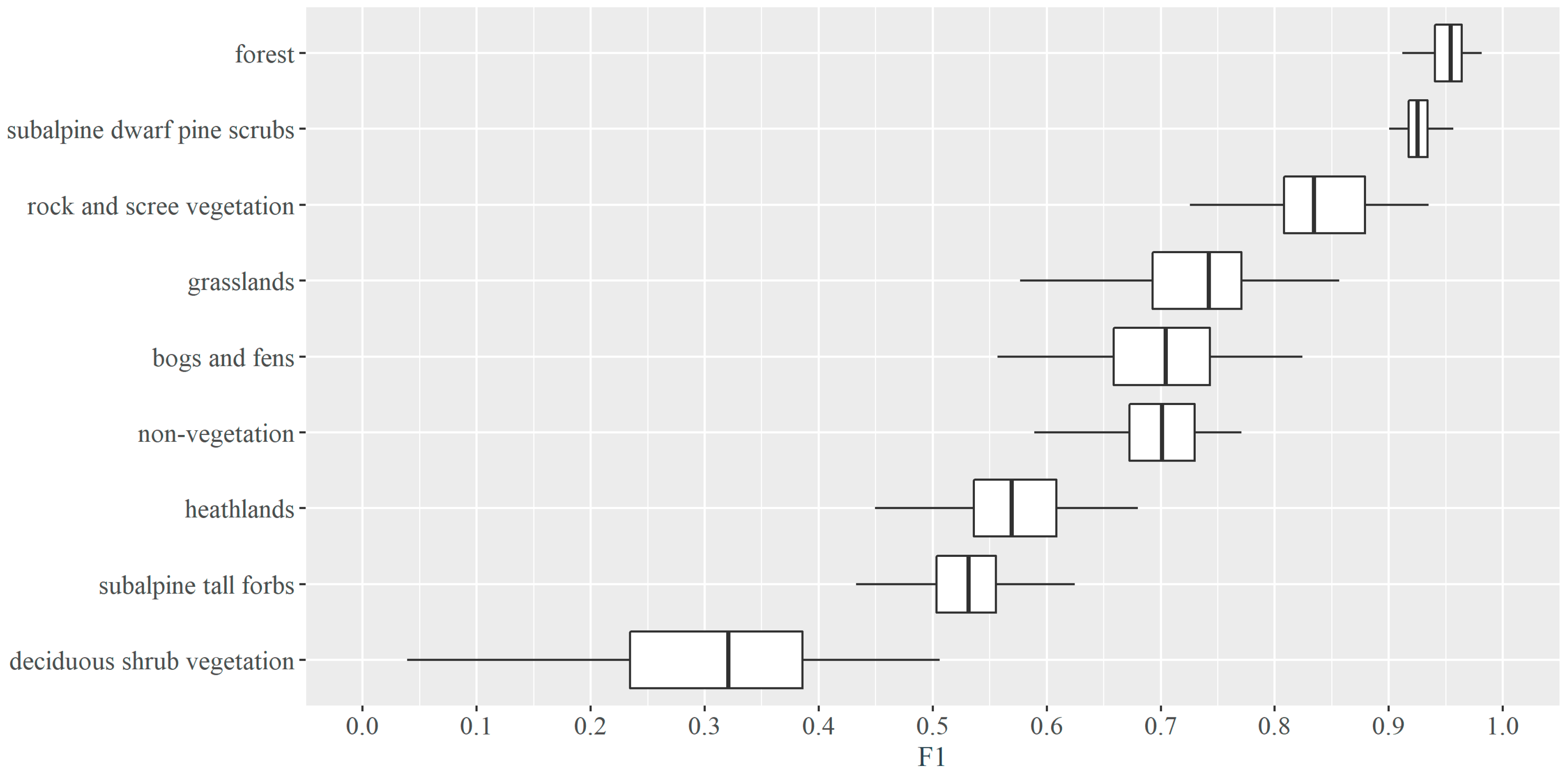
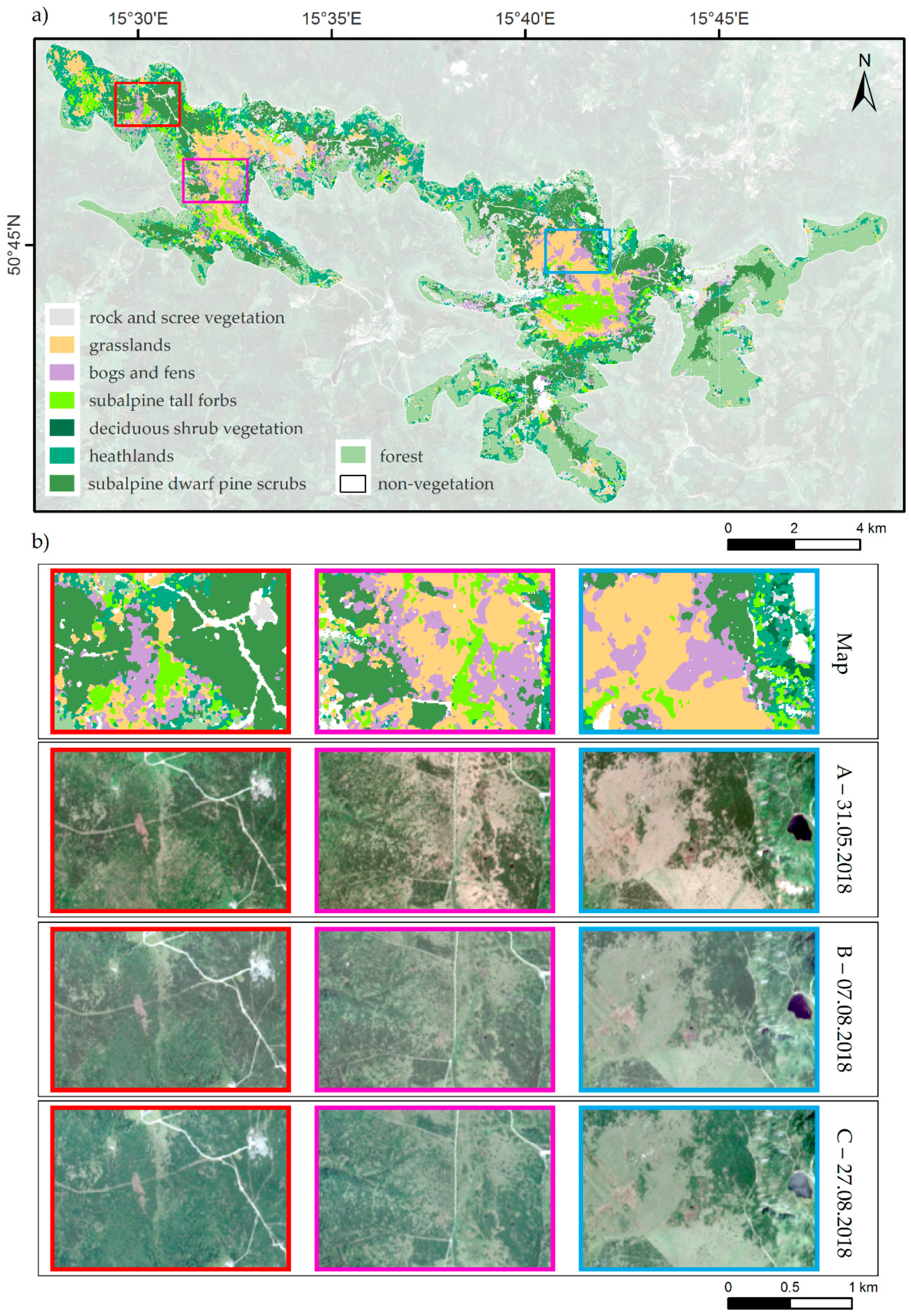
3.2. Vegetation Types Classification Results

The best-classified types of vegetation turned out to be forest and subalpine dwarf pine scrubs. Both classes reached a median of PA, UA, and F1 accuracies of around 90%—i.e., 94%, 89% (Figure 4), and 90% (Figure 5), respectively. Due to the high internal homogeneity, these classes also represent the greatest stability, which is confirmed by the small width of the distribution of achieved accuracy. Satisfactory results, above 60% of both accuracies and an F1 score above 70%, were also obtained for classes whose spectral characteristics constituted a specific mixture of signals, i.e., rock and scree vegetation and those characterized by unique physiognomy during subsequent stages of the growing season, i.e., grasslands. Deciduous shrubs were the worst classified type of vegetation, for which the median for both accuracies was less than 50% and F1 did not exceed 60%. For some classes, PA was lower than UA, because it was more difficult to fit the result with the validation data, e.g., for openwork and heterogeneous deciduous shrub vegetation class. For homogeneous classes like subalpine dwarf pine scrubs, this fit was simpler, and PA exceeded that of UA.
The analysis of the error matrix shows that the most frequently confusing class was deciduous shrub vegetation, which, in approximately 30% of cases, was classified as heathlands and in approximately 20% as subalpine tall forbs (Table 4). Physiognomically similar classes were confused quite often too—about 21% of the subalpine tall forbs’ areas were confused with grasslands and nearly 14% with heathlands.
The visual assessment of the final map confirms the accuracy obtained during the quantitative evaluation (Figure 6). The map of high-mountain vegetation created in the process of classification is largely similar to the reference map of non-forest vegetation [47]. The main differences concern the classes that obtained the lowest accuracy and which, because they are composed of heterogeneous complexes of communities with dominant species that are also species accompanying the other separations, have been mixed—i.e., the sites of heathlands, subalpine tall forbs, and deciduous shrub vegetation.

4. Discussion

Previous studies highlighted the advantages of single-date imagery in their vegetation classification for this mountain area [7,18,46]; however, our study goes further and demonstrates the advantage of using the freely available Sentinel-2 multi-temporal data for accurate vegetation mapping. We divided the discussion section into three parts: the first is devoted to mountain vegetation classification with special attention to the Giant Mountains study area (Section 4.1); in the second, we describe the use of multi-temporal data in classification (Section 4.2); in the third, we discuss the sense of including additional variables in the classification (Section 4.3).

4.1. Mountain Vegetation Classification

Image remote sensing has a great deal of potential for identifying types of mountain vegetation due to a wide range of available resolutions—spectral, spatial, and temporal, a properly generalized legend, and the selection of a classification algorithm adequate to the character of the data. The results obtained in this study (OA equal to 79.5%) show the usefulness of multispectral satellite data for the identification of types of high mountain vegetation. Other studies, which used comparable data, corresponding categories, and classification algorithms produced similar results, thus, confirming our results. Suchá et al. [45] classified eight vegetation types above the tree line in the Krkonoše Mts. National Park using Landsat-8 data (spatial resolution 30 m, seven spectral bands) and three per-pixel algorithm classifiers (ML, SVMs, and NNs) and obtained the best OA for ML classifier (78.3%). The study in [18] performed a similar investigation to ours, where eight types of vegetation were classified using simulated Sentinel-2 data and SVM classifier instead, which resulted in 81.9% OA for the dataset consisting of six bands as an effect of PCA and 78.3% OA for the total set of bands. Analogous studies with multispectral Sentinel-2 data were provided by Kupková et al. [7] where SVM, MLC, and NN algorithms were used to classify eight vegetation classes in Eastern tundra of the Giant Mountains, which yielded lower OAs than our results—71.0% and 79.5% based on SVM, respectively.
The complexity of the mountain vegetation means that the classification at a higher level of detail than the vegetation type requires the involvement of sensors registering images in many spectral bands, while also maintaining high spatial resolution. For this purpose, aerial hyperspectral data, such as AVIRIS (Airborne Visible/Infra-Red Imaging Spectrometer; 224 spectral bands), DAIS 7915 (Digital Airborne Imaging Spectrometer, 79 bands), AISA Dual (Airborne Imaging Spectrometer; 494 bands), or APEX (288 bands) data were employed [7,15,19]. These attributes allow to classify heterogeneous mountain vegetation at the community level and obtain high accuracy (74%–84% OA), despite its complicated structure; however, multispectral Sentinel-2 data also has the advantage of spectral resolution due to existence of SWIR, NIR, and red-edge bands, which was confirmed by a study of mountain vegetation [10] and other studies [28,30,32]. In our case, SWIR (11 and 12) and NIR (8a) bands were the most important in the classification of the entire ABCD dataset, which confirms the 20 first variables (Figure A2 in Appendix A). SWIR1 was the first most important variable for deciduous shrub vegetation; SWIR2 for grasslands, bogs and fens, heathlands, and subalpine tall forbs; and NIR (8a band) for forests and rock and scree vegetation. For subalpine dwarf pine scrub classification, the most important was NIR (7 band). Depending on the class, different bands were placed in the 20 most important bands in classification; however, for all classes except subalpine dwarf pine scrubs, SWIR bands from four different dates always occurred. To improve the classification model all used spectral bands could be correlated with each other to select only uncorrelated ones for further study. However, in most of the articles that discuss the use of SVM for vegetation classification, all available Sentinel bands (except the so-called “atmospheric” bands) are used [7,60,61].
The complex character of the classified vegetation types causes divergent results. Large-area forests and subalpine dwarf pine scrubs growing in homogeneous patches turned out to be the most identifiable classes, reaching medians of PA and UA above the 90% (forest: PA—95.0%; UA—96.5%; subalpine dwarf pine scrubs: PA—95.2%; UA—90.0%). The specific texture of the subalpine dwarf pine scrubs and the characteristic spectral reflection of mosaics of forest-forming species makes them one of the best-classified types of alpine vegetation. Similar results, where PA and UA accuracies fluctuated around 90%, were obtained by other authors classifying subalpine dwarf pine scrubs and forests on Landsat-8 [45], Sentinel-2 [7,18], the Environmental Mapping and Analysis Program (EnMAP) [18,46], APEX [7,15,46], and AISA Dual [7] data. Among the best-classifying types of vegetation, rock and scree vegetation was also frequently mentioned, which is well distinguishable even by sensors with a spatial resolution of no more than 10 m, i.e., Sentinel-2: PA—91.5%, UA—87.0% [18] and PA—92.7%, UA—95.0% [7] or EnMAP: PA—97.5%, UA—96.3% [18]. The clue is the fact of mixing the signal from plants and rocks, which results in a high reflectance in NIR and SWIR bands. In our work, it was the third best-classified type of vegetation, achieving a PA and UA of 83.0% and 88.1%, respectively. On the other hand, classes with heterogeneous community complexes proved to be the worst-classified types of vegetation, with an accuracy not exceeding 60%, whose dominant species are often also accompanying species of other types—i.e., heathlands (PA—60.3%, UA—55.2%) and subalpine tall forbs (PA—54.9%, UA—52.8%) and those that form too small clusters to be well distinguishable by the sensor—i.e., deciduous shrub vegetation (PA—25.6%, UA—41.0%). Subalpine tall forbs and heathlands, due to their high spectral similarity, practically prevent proper separation on multispectral data—in Landsat-8, the OA often does not exceed 50% [45], and in the case of Sentinel-2, the OA often does not exceed 60% [7,18]. Higher values are obtained for classifications based on hyperspectral data, where PA and UA reach a 70% of OA, i.e., EnMAP: PA—79.2%, UA—67.9% (subalpine tall forbs), and PA—44.8%, UA—52.0% (heathlands) [46], or AISA Dual: PA—85.1%, UA—85.8% (subalpine tall forbs), and PA—81.6%, UA—83.8% (heathlands) [7].
Table 2 shows that the datasets for classification were not balanced. It was also noted by other authors as a problem affecting the accuracy of machine learning [16,17]. Our results show this effect in the most and least numerous classes as subalpine dwarf pine scrubs and deciduous shrub vegetation, respectively; however, for forests and rock and scree vegetation mentioned above also occupied by smaller areas (closer to the least than the most numerous) the accuracies were some of the highest. Balancing the dataset, particularly in the natural vegetation area, is not as straightforward as confirmed by other authors [6,29,30]; however, Thanh Noi and Kappas [17] proved that for SVM, in comparison to random forest (RF) and k-nearest neighbor (k-NN), the difference between various sample sizes was insignificant, which can support our method choice and obtained results, and we conclude that this effect was not very pronounced.

4.2. Multi-Temporal Classification

The main aspect working in favor of Sentinel-2 data, in addition to its open-access character, is the high temporal resolution enabling the generation of multi-temporal compositions. Taking into account the images in which successive stages of vegetation were captured, it is possible to obtain much better classification results compared to the results based on single-date data. The results obtained in this study confirm that each of the analyzed multi-temporal compositions, two, three, or four dates, resulted in a higher value of OA concerning the classification on single-date data—the highest value for single-date data was 74.2%, whereas the lowest value for multi-temporal composition was 76.3%. A similar tendency, regardless of the sensor and used algorithm, can also be observed for other objects of the study, i.e., land cover [62], tree species [28,29,30,31], swamp [25], and grassy [27,33] and shrubby [6] communities (Table 5).
Selecting the optimal composition that generates the highest accuracy is complex. The quality of the composition is influenced by both the number of images that comprise it and the date of registration. It was shown that at some stage, the addition of further images does not cause a further increase in accuracy, and the stabilization of the result depends largely on the dates taken into account [27,38]. In our study, the highest OA was obtained for a composition consisting of three images (79.5%) out of four available (78.5%). Similarly, in the study where shrub communities were classified, despite the access to four images (12% OA), a composition using only two of them resulted in a higher accuracy (68% OA) [6]. In the case of classification of tree species, where authors had access to 18 images, the composition with five images obtained the highest result—92.1% and 92.4% OA, respectively [29].
The key assumption in multi-temporal classification is that the vegetation varies between different terms of data acquisition within a year when using inter-seasonal data. When there is not enough spectral information to divide spectrally similar groups of vegetation, even with SWIR or NIR regions registered by Sentinel-2, the use of temporal information as additional variables demonstrates the advantage of the approach proposed in this work. The registration dates of the images constituting the multi-temporal composition are the key issue determining the quality of the obtained results. A satisfactory classification result largely depends on the characteristics of the studied vegetation and its phenological cycle. By capturing those periods of the year in which key stages of a plant life cycle are observable, it is possible to generate compositions that produce the best results. In most cases, compositions including the contrast of spring and autumn are considered to be the most informative because it is the time of intensified discoloration associated with flowering and senescence of vegetation [6,28,29]. Slightly less often, especially in the case of grassy vegetation, early and late summer are also indicated, i.e., the period of dynamic growth [27,63]. In the case of high-mountain vegetation, which is the subject of this study, the composition generating the highest result (79.5%) was composed of spring (31 May) and late summer (07 August, 27 August) images. In this case, grasslands that discolor as a result of drying are the most important indicator for the separation of different types of vegetation [7,15,45]. Additional variable importance analysis performed for the ABCD dataset revealed that, for all classes, the most numerous important features located at the first 20 places were from A, B, and C datasets (Figure A2 in Appendix A). The spectral band from spring was indicated as the most important for subalpine dwarf pine scrubs, grasslands, heathlands, and deciduous shrub vegetation; the band from the B dataset was the best in the classification of forests and rock and scree vegetation; and band from C dataset was the best in the classification for bogs and fens and subalpine tall forbs.

4.3. Additional Variables

Apart from different factors, e.g., sensor, legend generalization, algorithm, or the number of images analyzed, the impact on the obtained classification result also has additional processing. It includes those that reduce spectral space (transformations), and also those that increase the information capacity in the form of vegetation indices added as new bands. The transformation was performed to extract key information that differentiates the analyzed classes. Although in many studies this procedure resulted in an increase of the OA—AISA Eagle II from 72.8% to 82.1% (minimum noise fraction transformation; MNF) [9]; AISA Dual from 74.2% to 84.3%, APEX from 77.7% to 82.6% (PCA) [7]; Sentinel-2 from 78.3% to 81.9% (PCA) [18]—in our work, the PCA transformation reduced the final result by slightly more than 2 pp. (from 79.5% to 77.1%); however, this is not an exception, because there are also studies in which transformations led to lower accuracies—APEX from 82.7% to 81.0% (PCA) [15]; EnMAP from 82.9% to 56.3% (PCA) [18]; Sentinel-2 from 72.0% to 51.0% (PCA) [6]. Calculation of the most important variables in the classification of the ABC_PCA dataset allowed us to confirm this conclusion because only two/three PCA bands were placed in 20 top variables for each vegetation type classification (Figure A3 in Appendix A). In the analysis of individual classes, in the first place, PCA bands were noted for rock and scree vegetation, bogs and fens, and subalpine tall forbs. Overall, from the 10 calculated PCA bands only 4 occurred in these 20 most important variables, and the most frequently occurring PC1 and PC2 bands.
When including vegetation indices as an input to the classification of multispectral data to increase its quality as, e.g., in forest species classification improving the model performance by around five percentage points [30], in our study it led to a decrease in the OA from 79.5% to 79.2%; however, in the variable importance analysis of the ABC_IND dataset, we noted that in most cases, they were located in the top-20 variables, and for each class, at the first place vegetation index was located (Figure A4 in Appendix A). The most frequently occurring were EVI and VARI, based on VIS (visible) + NIR and only VIS spectral bands, respectively, but band 11 from SWIR was similarly frequent. For five classes, the first most important variable was ReNDVI (forest, rock and scree vegetation, grasslands, heathlands, and deciduous shrub vegetation) supporting the importance of red-edge in combination with the NIR band. Many publications described strategically selected spectral ranges of Sentinel-2 data [6,28,41,64]. This multispectral satellite, registering the electromagnetic spectrum in 13 spectral ranges, has several narrow (less than 20 nm) bands. As a consequence, the only spectral bands themselves can generate higher results than sets enriched with secondary information from, e.g., vegetation indices. In a study where grassland species were the authors only analyzed the classification of spectral bands, they were able to reach 90.4% OA, whereas with NDVI, they were able to reach 88.6% [41]. Another research, describing shrubs classification, reported 72.0% OA for only spectral bands and 59.0% for a dataset consisting of spectral bands, NDVI, and PCA [6].
Based on our results and additional analysis of important variables in classification (Figure A2, Figure A3 and Figure A4 in Appendix A), this study can be investigated further to create the most optimal models with only uncorrelated spectral bands after correlation analysis and with the best variables after feature selection. However, as our study aim stated, we wanted to assess the potential of Sentinel-2 multi-temporal data for mountain vegetation types classification by analyzing plant phenology differences through the growing season; hence, here we decided to use whole datasets to recommend the best dates for creating a multi-temporal composition.

5. Conclusions

The presented problem of mountain vegetation types mapping in the Giant Mountains allowed us to determine the usefulness of Sentinel-2 multi-temporal satellite data. Analysis of the obtained results led to the following conclusions:
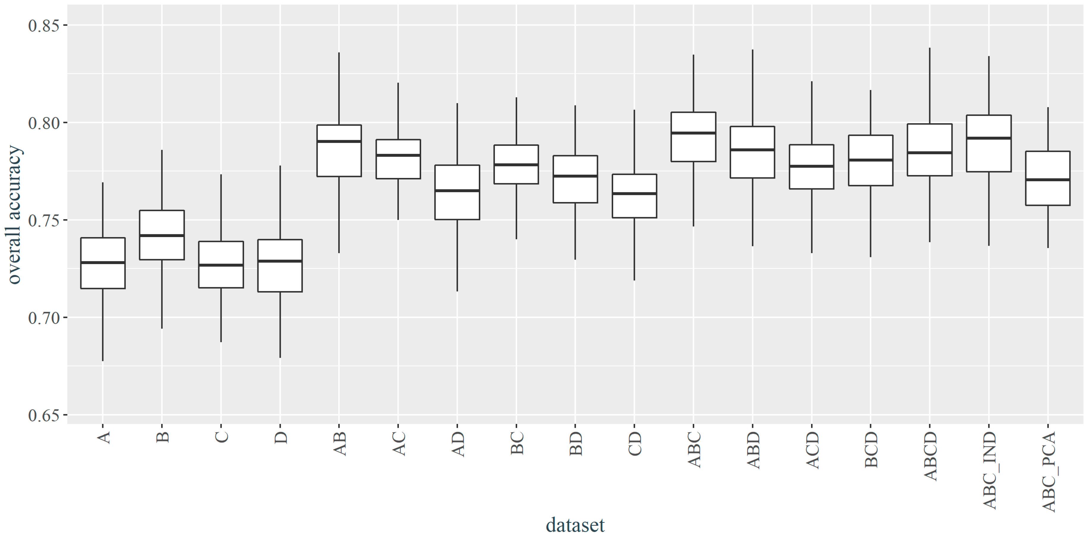
  • Sentinel-2 multispectral data allow us to classify high-mountain vegetation at a satisfactory level of accuracy, assuming the right level of generalization of the legend, the selection of a classification algorithm adequate to the character of the data, and the use of the advantages associated with high temporal resolution—classification based on multi-temporal compositions allows achieving better results compared to the results generated based on single-date data. Contrary to high-accuracy hyperspectral data not fully available at this moment even for single-date collection and limited for use in local-scale analysis, Sentinel-2 data can be assessed as more applicable.
  • The quality of the temporal composition, in addition to the number of images, is primarily due to the date of acquisition—compositions containing contrasting spring and autumn, i.e., the time of intensified discoloration associated with flowering and senescence vegetation, were considered to be the most informative. Lower OA of a single image does not exclude it as a valuable component of the multi-temporal composition, as after adding an image from late August gave better accuracies than the two preceding images from the beginning of August and the end of May.
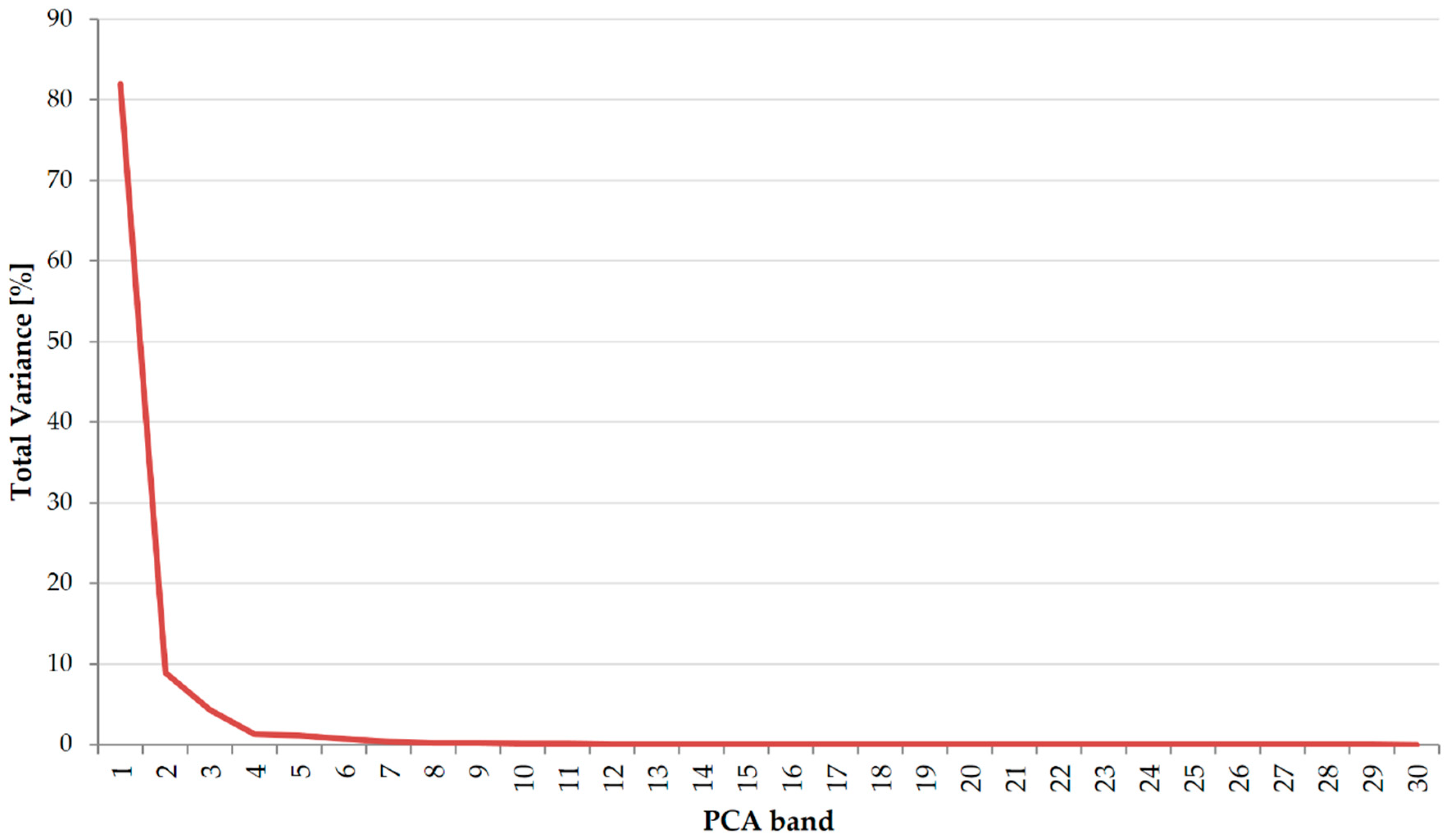
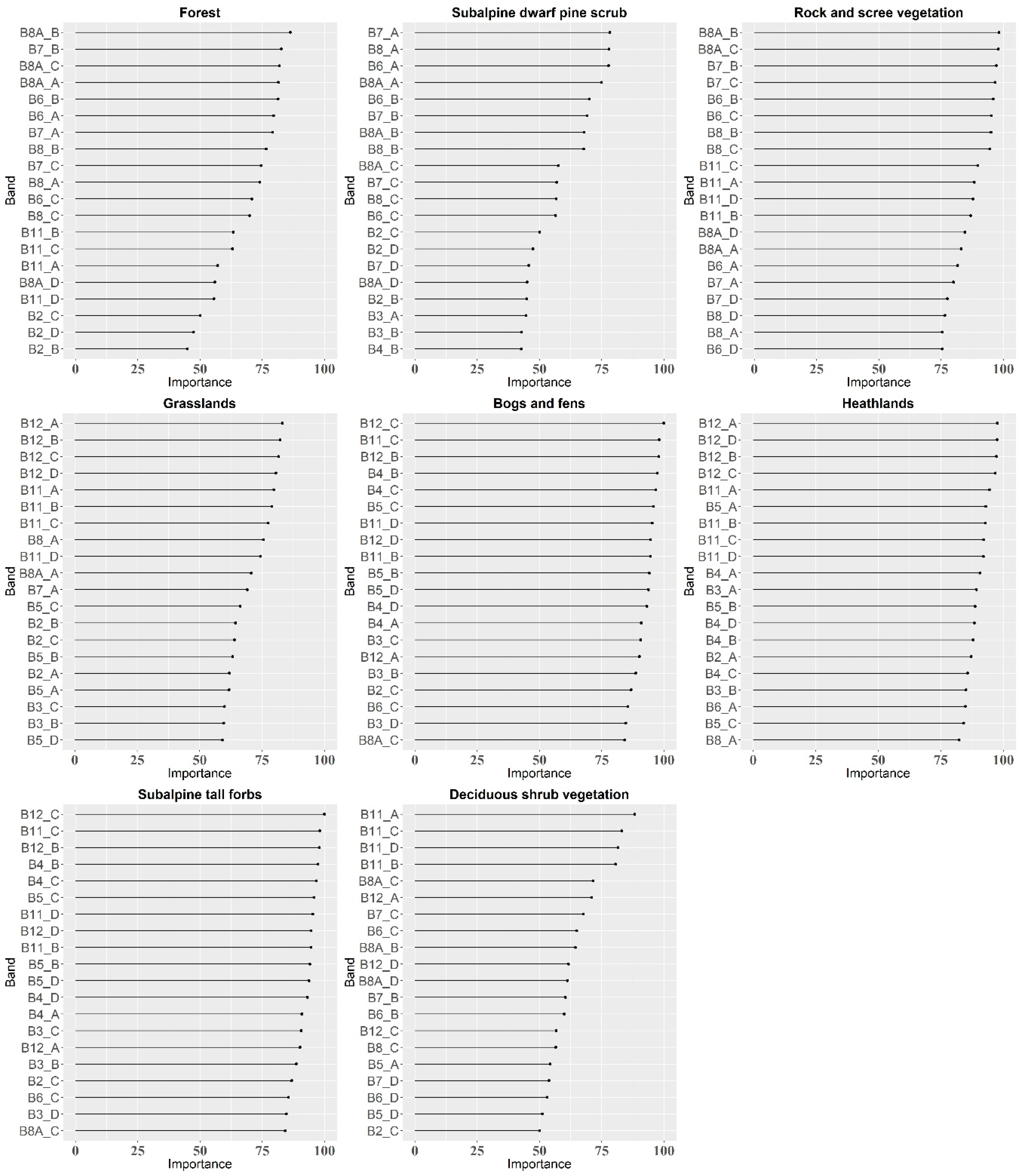
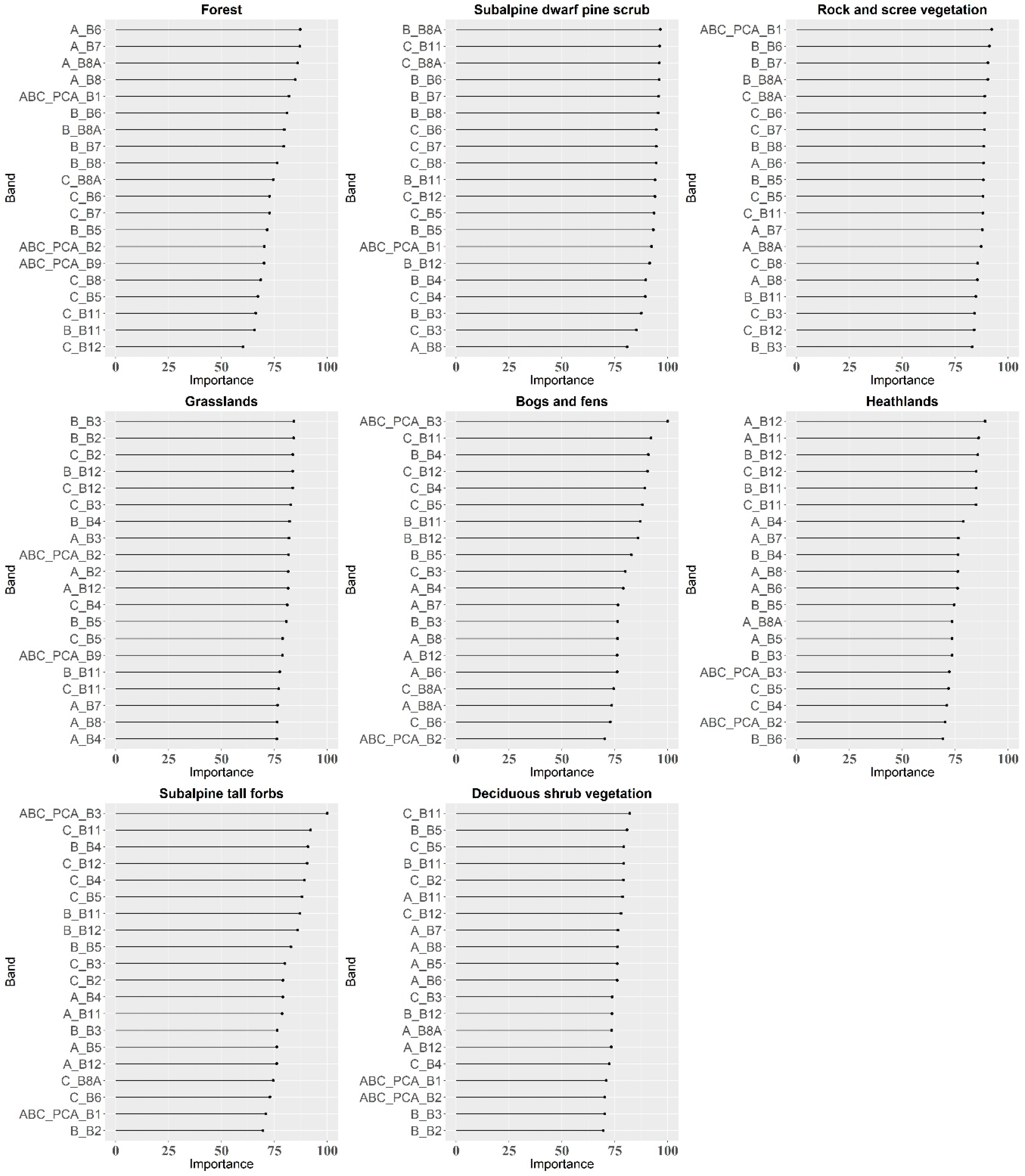
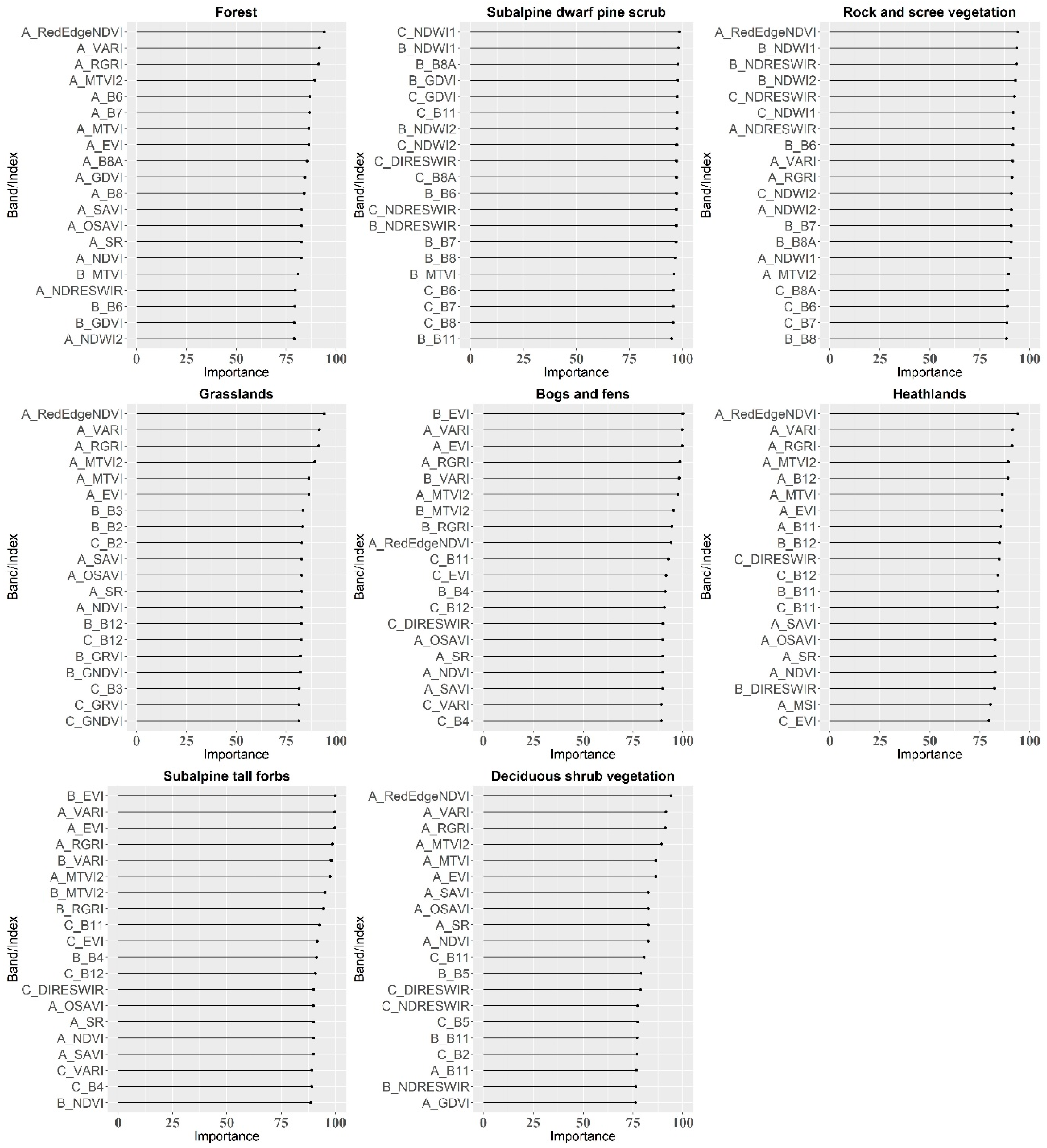
  • The additional variables (vegetation indices and PCA transformation bands) tested on the best-classified dataset did not contribute to the increase in OA, which suggests that in the case of the classification of multi-temporal Sentinel-2 data, the most important variables for a satisfactory result are the images themselves (number and dates of acquisition), not their additional processing; however, the inclusion of vegetation indices can be investigated more deeply, taking into account the most influential indices for particular vegetation types classification to build the models based on only the most informative features.
The map of mountain vegetation types in the Giant Mountains developed based on Sentinel-2 data is an objective source of information that can support monitoring works, especially because the high temporal resolution, ensuring access to constantly supplemented data resources, enables its continuous updating.

Author Contributions

Conceptualization, A.M.-O.; methodology, A.M.-O., and M.W.; validation, M.W., and A.M.-O.; formal analysis, A.M.-O.; investigation, M.W. and A.M.-O.; resources, A.M.-O.; writing—original draft preparation, M.W., and A.M.-O.; writing—review and editing, A.M.-O., and M.W.; visualization, M.W.; supervision, A.M.-O.; funding acquisition, A.M.-O. All authors have read and agreed to the published version of the manuscript.

Funding

This research received no external funding. The APC was funded by the Faculty of Geography and Regional Studies, University of Warsaw.

Acknowledgments

The authors wish to thank EUFAR, DLR and VITO for APEX data acquisition in 2012. We are also grateful to Lidia Przewoźnik, Bronisław Wojtuń, and Bogdan Zagajewski for their support in field data collection and to both national parks authorities for giving the access to provide this research. We are also grateful to Reviewers and Editor, who allowed us to improve the manuscript.

Conflicts of Interest

The authors declare no conflict of interest.

Appendix A

Table A1. Vegetation indices used in the study (bold numbers in formulas indicate individual Sentinel-2 bands).
No.AbbreviationNameFormula for Sentinel-2 data
1EVIEnhanced Vegetation IndexEVI = 2.5 × (8 − 5)/(8 + 6 × 5 − 7.5 × 2) + 1
2GDVIGreen Difference Vegetation IndexGDVI = 83
3GNDVIGreen Normalized Difference Vegetation IndexGNDVI = 83/9 + 3
4GRVIGreen Ratio Vegetation IndexGRVI = 8/3
5MSIMoisture Stress IndexMSI = 11/8
6MTVI1Modified Triangular Vegetation IndexMTVI1 = 1.2 (1.2 (83) − 2.5 (43))
7MTVI2Modified Triangular Vegetation Index - ImprovedMTVI2 = 1.5 (1.2 (83) − 2.5 (43))(√(2 × 8 + 1)2 − (6 × 8 − 5√4) − 0.5)
8NDRESWIRNormalized Difference Red-Edge and SWIR2NDRESWIR = 612/6 + 12
9NDVINormalized Difference Vegetation IndexNDVI = 84/8 + 4
10NDWI1Normalized Difference Water Index 1NDWI1 = 811/8 + 11
11NDWI2Normalized Difference Water Index 2NDWI2 = 812/8 + 12
12OSAVIOptimized Soil Adjusted Vegetation IndexOSAVI = (1 + 0.16) 84/8 + 4 + 0.16
13reNDVIRed Edge Normalized Difference Vegetation IndexNDVI 705 = 85/8 + 5
14RGRIRed Green Ratio IndexRGRI = 5/3
15DIRESWIRRed SWIR1 DifferenceDIRESWIR = 411
16SAVISoil Adjusted Vegetation IndexSAVI = 1.5 (84) 8 + 4 + 0.5
17SRSimple RatioSR = 8/4
18VARIVisible Atmospherically Resistant IndexVARI = 34/3 + 42
Table A2. Correlation table of variables used to PCA transformation bands selection.
Band123456789101112131415161718192021222324252627282930
110.90.90.80.40.30.30.30.60.80.80.70.70.60.40.30.30.30.50.60.70.70.70.60.40.30.30.30.50.5
20.910.90.90.60.50.50.50.80.80.80.80.70.80.60.50.60.50.70.70.80.80.70.80.60.50.50.50.60.7
30.90.910.80.30.20.20.20.70.80.80.70.70.70.40.30.30.30.50.60.70.70.70.60.40.30.30.30.50.6
40.80.90.810.70.60.60.60.90.90.70.80.70.90.70.70.60.70.80.80.70.80.70.90.70.60.60.60.80.8
50.40.60.30.711110.80.60.50.60.50.70.90.90.90.90.80.70.50.60.50.70.90.90.80.90.80.7
60.30.50.20.611110.70.50.40.60.50.70.90.90.90.90.80.70.40.60.50.70.90.80.80.90.80.7
70.30.50.20.611110.70.50.40.60.50.70.90.90.90.90.80.60.40.60.50.70.80.80.80.80.70.6
80.30.50.20.611110.80.60.40.60.50.70.90.90.90.90.80.70.40.60.50.70.90.90.80.90.80.7
90.60.80.70.90.80.70.70.8110.70.80.70.90.80.80.70.80.90.90.70.80.70.90.80.70.70.70.90.9
100.80.80.80.90.60.50.50.6110.70.80.80.80.70.60.60.60.80.80.70.80.80.80.60.60.50.60.80.8
110.80.80.80.70.50.40.40.40.70.71110.80.50.40.40.40.70.80.90.90.90.80.50.40.40.40.70.8
120.70.80.70.80.60.60.60.60.80.8110.90.90.70.60.60.60.80.90.910.90.90.70.60.60.60.80.9
130.70.70.70.70.50.50.50.50.70.810.910.90.50.40.40.40.80.90.90.910.90.50.40.40.40.80.9
140.60.80.70.90.70.70.70.70.90.80.80.90.910.80.70.70.70.90.90.80.90.910.70.70.60.70.90.9
150.40.60.40.70.90.90.90.90.80.70.50.70.50.8110.910.80.70.50.70.50.8110.910.80.7
160.30.50.30.70.90.90.90.90.80.60.40.60.40.711110.70.60.40.60.50.7110.910.70.6
170.30.60.30.60.90.90.90.90.70.60.40.60.40.70.91110.70.60.40.60.50.70.90.910.90.70.6
180.30.50.30.70.90.90.90.90.80.60.40.60.40.711110.80.60.40.60.50.7110.910.70.6
190.50.70.50.80.80.80.80.80.90.80.70.80.80.90.80.70.70.8110.70.80.80.90.80.70.70.711
200.60.70.60.80.70.70.60.70.90.80.80.90.90.90.70.60.60.6110.80.90.90.90.60.60.50.611
210.70.80.70.70.50.40.40.40.70.70.90.90.90.80.50.40.40.40.70.81110.80.50.40.40.40.70.8
220.70.80.70.80.60.60.60.60.80.80.910.90.90.70.60.60.60.80.91110.90.70.60.60.60.80.9
230.70.70.70.70.50.50.50.50.70.80.90.910.90.50.50.50.50.80.91110.90.50.40.40.40.80.9
240.60.80.60.90.70.70.70.70.90.80.80.90.910.80.70.70.70.90.90.80.90.910.80.70.70.70.90.9
250.40.60.40.70.90.90.80.90.80.60.50.70.50.7110.910.80.60.50.70.50.8110.910.70.6
260.30.50.30.60.90.80.80.90.70.60.40.60.40.7110.910.70.60.40.60.40.7110.910.70.6
270.30.50.30.60.80.80.80.80.70.50.40.60.40.60.90.910.90.70.50.40.60.40.70.90.910.90.70.5
280.30.50.30.60.90.90.80.90.70.60.40.60.40.7110.910.70.60.40.60.40.7110.910.70.6
290.50.60.50.80.80.80.70.80.90.80.70.80.80.90.80.70.70.7110.70.80.80.90.70.70.70.711
300.50.70.60.80.70.70.60.70.90.80.80.90.90.90.70.60.60.6110.80.90.90.90.60.60.50.611
Figure A1. Total variance explained by each PCA band of ABC dataset.
Remotesensing 12 02696 g0a1
Figure A2. The 20 most important variables in classification of each vegetation type using ABCD dataset.
Remotesensing 12 02696 g0a2
Figure A3. The 20 most important variables in classification of each vegetation type using ABC_PCA dataset.
Remotesensing 12 02696 g0a3
Figure A4. The 20 most important variables in classification of each vegetation type using ABC_IND dataset.
Remotesensing 12 02696 g0a4

References

  1. Reese, H.; Nordkvist, K.; Nyström, M.; Bohlin, J.; Olsson, H. Combining point clouds from image matching with SPOT 5 multispectral data for mountain vegetation classification. Int. J. Remote Sens. 2015. [Google Scholar] [CrossRef]
  2. Żołnierz, L.; Wojtuń, B.; Przewoźnik, L. Ekosystemy Nieleśne Karkonoskiego Parku Narodowego; Karkonoski Park Narodowy: Jelenia Góra, Poland, 2012. [Google Scholar]
  3. Xie, Y.; Sha, Z.; Yu, M. Remote sensing imagery in vegetation mapping: A review. J. Plant Ecol. 2008, 1, 9–23. [Google Scholar] [CrossRef]
  4. Osińska-Skotak, K.; Radecka, A.; Piórkowski, H.; Michalska-Hejduk, D.; Kopeć, D.; Tokarska-Guzik, B.; Ostrowski, W.; Kania, A.; Niedzielko, J. Mapping Succession in Non-Forest Habitats by Means of Remote Sensing: Is the Data Acquisition Time Critical for Species Discrimination? Remote Sens. 2019, 11, 2629. [Google Scholar] [CrossRef] [Green Version]
  5. Sławik, Ł.; Niedzielko, J.; Kania, A.; Piórkowski, H.; Kopeć, D. Multiple flights or single flight instrument fusion of hyperspectral and ALS data? A comparison of their performance for vegetation mapping. Remote Sens. 2019, 11, 913. [Google Scholar] [CrossRef] [Green Version]
  6. Macintyre, P.; van Niekerk, A.; Mucina, L. Efficacy of multi-season Sentinel-2 imagery for compositional vegetation classification. Int. J. Appl. Earth Obs. Geoinf. 2020, 85, 101980. [Google Scholar] [CrossRef]
  7. Kupková, L.; Červená, L.; Suchá, R.; Jakešová, L.; Zagajewski, B.; Březina, S.; Albrechtová, J. Classification of tundra vegetation in the Krkonoše Mts. National park using APEX, AISA dual and sentinel-2A data. Eur. J. Remote Sens. 2017, 50, 29–46. [Google Scholar] [CrossRef]
  8. Sabat-Tomala, A.; Raczko, E.; Zagajewski, B. Comparison of support vector machine and random forest algorithms for invasive and expansive species classification using airborne hyperspectral data. Remote Sens. 2020, 12, 516. [Google Scholar] [CrossRef] [Green Version]
  9. Burai, P.; Deák, B.; Valkó, O.; Tomor, T. Classification of herbaceous vegetation using airborne hyperspectral imagery. Remote Sens. 2015, 7, 2046–2066. [Google Scholar] [CrossRef] [Green Version]
  10. Adagbasa, E.G.; Adelabu, S.A.; Okello, T.W. Application of deep learning with stratified K-fold for vegetation species discrimation in a protected mountainous region using Sentinel-2 image. Geocarto Int. 2019. [Google Scholar] [CrossRef]
  11. Vapnik, V.N. An overview of statistical learning theory. IEEE Trans. Neural Networks 1999, 10, 988–999. [Google Scholar] [CrossRef] [Green Version]
  12. Foody, G.M.; Mathur, A. Toward intelligent training of supervised image classifications: Directing training data acquisition for SVM classification. Remote Sens. Environ. 2004, 93, 107–117. [Google Scholar] [CrossRef]
  13. Waske, B.; van der Linden, S.; Benediktsson, J.A.; Rabe, A.; Hostert, P. Sensitivity of Support Vector Machines to Random Feature Selection in Classification of Hyperspectral Data. IEEE Trans. Geosci. Remote Sens. 2010, 48, 2880–2889. [Google Scholar] [CrossRef] [Green Version]
  14. Demarchi, L.; Canters, F.; Cariou, C.; Licciardi, G.; Chan, J.C.-W. Assessing the performance of two unsupervised dimensionality reduction techniques on hyperspectral APEX data for high resolution urban land-cover mapping. ISPRS J. Photogramm. Remote Sens. 2014, 87, 166–179. [Google Scholar] [CrossRef]
  15. Marcinkowska-Ochtyra, A.; Zagajewski, B.; Raczko, E.; Ochtyra, A.; Jarocińska, A. Classification of high-mountain vegetation communities within a diverse Giant Mountains ecosystem using airborne APEX hyperspectral imagery. Remote Sens. 2018, 10, 570. [Google Scholar] [CrossRef] [Green Version]
  16. Akbani, R.; Kwek, S.; Japkowicz, N. Applying Support Vector Machines to Imbalanced Datasets. In Lecture Notes in Artificial Intelligence (Subseries of Lecture Notes in Computer Science); Springer: Berlin/Heidelberg, Germany, 2004; pp. 39–50. [Google Scholar]
  17. Thanh Noi, P.; Kappas, M. Comparison of Random Forest, k-Nearest Neighbor, and Support Vector Machine Classifiers for Land Cover Classification Using Sentinel-2 Imagery. Sensors 2017, 18, 18. [Google Scholar] [CrossRef] [Green Version]
  18. Jędrych, M.; Zagajewski, B.; Marcinkowska-Ochtyra, A. Application of Sentinel-2 and EnMAP new satellite data to the mapping of alpine vegetation of the Karkonosze Mountains. Pol. Cartogr. Rev. 2017, 49, 107–119. [Google Scholar] [CrossRef] [Green Version]
  19. Kokaly, R.F.; Despain, D.G.; Clark, R.N.; Livo, K.E. Mapping vegetation in Yellowstone National Park using spectral feature analysis of AVIRIS data. Remote Sens. Environ. 2003, 84, 437–456. [Google Scholar] [CrossRef] [Green Version]
  20. Chan, J.C.W.; Paelinckx, D. Evaluation of Random Forest and Adaboost tree-based ensemble classification and spectral band selection for ecotope mapping using airborne hyperspectral imagery. Remote Sens. Environ. 2008. [Google Scholar] [CrossRef]
  21. Raczko, E.; Zagajewski, B. Tree species classification of the UNESCO man and the biosphere Karkonoski National Park (Poland) using artificial neural networks and APEX hyperspectral images. Remote Sens. 2018, 10, 1111. [Google Scholar] [CrossRef] [Green Version]
  22. Dehaan, R.; Louis, J.; Wilson, A.; Hall, A.; Rumbachs, R. Discrimination of blackberry (Rubus fruticosus sp. agg.) using hyperspectral imagery in Kosciuszko National Park, NSW, Australia. ISPRS J. Photogramm. Remote Sens. 2007. [Google Scholar] [CrossRef]
  23. Cingolani, A.M.; Renison, D.; Zak, M.R.; Cabido, M.R. Mapping vegetation in a heterogeneous mountain rangeland using landsat data: An alternative method to define and classify land-cover units. Remote Sens. Environ. 2004. [Google Scholar] [CrossRef]
  24. Kopeć, D.; Zakrzewska, A.; Halladin-Dąbrowska, A.; Wylazłowska, J.; Kania, A.; Niedzielko, J. Using Airborne Hyperspectral Imaging Spectroscopy to Accurately Monitor Invasive and Expansive Herb Plants: Limitations and Requirements of the Method. Sensors 2019, 19, 2871. [Google Scholar] [CrossRef] [PubMed] [Green Version]
  25. Rapinel, S.; Bouzillé, J.B.; Oszwald, J.; Bonis, A. Use of bi-Seasonal Landsat-8 Imagery for Mapping Marshland Plant Community Combinations at the Regional Scale. Wetlands 2015. [Google Scholar] [CrossRef]
  26. Díaz Varela, R.A.; Ramil Rego, P.; Calvo Iglesias, S.; Muñoz Sobrino, C. Automatic habitat classification methods based on satellite images: A practical assessment in the NW Iberia coastal mountains. Environ. Monit. Assess. 2008. [Google Scholar] [CrossRef] [PubMed]
  27. Rapinel, S.; Mony, C.; Lecoq, L.; Clément, B.; Thomas, A.; Hubert-Moy, L. Evaluation of Sentinel-2 time-series for mapping floodplain grassland plant communities. Remote Sens. Environ. 2019. [Google Scholar] [CrossRef]
  28. Persson, M.; Lindberg, E.; Reese, H. Tree Species Classification with Multi-Temporal Sentinel-2 Data. Remote Sens. 2018, 10, 1794. [Google Scholar] [CrossRef] [Green Version]
  29. Grabska, E.; Hostert, P.; Pflugmacher, D.; Ostapowicz, K. Forest stand species mapping using the sentinel-2 time series. Remote Sens. 2019, 11, 1197. [Google Scholar] [CrossRef] [Green Version]
  30. Immitzer, M.; Neuwirth, M.; Böck, S.; Brenner, H.; Vuolo, F.; Atzberger, C. Optimal Input Features for Tree Species Classification in Central Europe Based on Multi-Temporal Sentinel-2 Data. Remote Sens. 2019, 11, 2599. [Google Scholar] [CrossRef] [Green Version]
  31. Hościło, A.; Lewandowska, A. Mapping Forest Type and Tree Species on a Regional Scale Using Multi-Temporal Sentinel-2 Data. Remote Sens. 2019, 11, 929. [Google Scholar] [CrossRef] [Green Version]
  32. Puletti, N.; Chianucci, F.; Castaldi, C. Use of Sentinel-2 for forest classification in Mediterranean environments. Ann. Silvic. Res. 2018. [Google Scholar] [CrossRef]
  33. Hunter, F.D.L.; Mitchard, E.T.A.; Tyrrell, P.; Russell, S. Inter-seasonal time series imagery enhances classification accuracy of grazing resource and land degradation maps in a savanna ecosystem. Remote Sens. 2020, 12, 198. [Google Scholar] [CrossRef] [Green Version]
  34. Oldeland, J.; Dorigo, W.; Lieckfeld, L.; Lucieer, A.; Jürgens, N. Combining vegetation indices, constrained ordination and fuzzy classification for mapping semi-natural vegetation units from hyperspectral imagery. Remote Sens. Environ. 2010, 114, 1155–1166. [Google Scholar] [CrossRef]
  35. Hotelling, H. Analysis of a complex of statistical variables into principal components. J. Educ. Psychol. 1933. [Google Scholar] [CrossRef]
  36. Kauth, R.J.; Thomas, G.S. The tasseled cap-A graphic description of the spectral-temporal development of agricultural crops as seen by Landsat. In Proceedings of the Symposium on Machine Processing of Remotely Sensed Data, West Lafayette, IN, USA, 29 June–1 July 1976. [Google Scholar]
  37. Rouse, J.W.; Haas, R.H.; Schell, J.A.; Deering, D.W. Monitoring the vernal advancement and retrogradation (green wave effect) of natural vegetation. Prog. Rep. 1973. RSC 1978-4. [Google Scholar]
  38. Schuster, C.; Schmidt, T.; Conrad, C.; Kleinschmit, B.; Förster, M. Grassland habitat mapping by intra-annual time series analysis—Comparison of RapidEye and TerraSAR-X satellite data. Int. J. Appl. Earth Obs. Geoinf. 2015, 34, 25–34. [Google Scholar] [CrossRef]
  39. Demarchi, L.; Kania, A.; Ciezkowski, W.; Piórkowski, H.; Oświecimska-Piasko, Z.; Chormański, J. Recursive feature elimination and random forest classification of natura 2000 grasslands in lowland river valleys of poland based on airborne hyperspectral and LiDAR data fusion. Remote Sens. 2020, 12, 1842. [Google Scholar] [CrossRef]
  40. Marcinkowska-Ochtyra, A.; Jarocińska, A.; Bzdȩga, K.; Tokarska-Guzik, B. Classification of expansive grassland species in different growth stages based on hyperspectral and LiDAR data. Remote Sens. 2018, 10, 2019. [Google Scholar] [CrossRef] [Green Version]
  41. Shoko, C.; Mutanga, O. Examining the strength of the newly-launched Sentinel 2 MSI sensor in detecting and discriminating subtle differences between C3 and C4 grass species. ISPRS J. Photogramm. Remote Sens. 2017. [Google Scholar] [CrossRef]
  42. Marcinkowska-Ochtyra, A.; Gryguc, K.; Ochtyra, A.; Kopeć, D.; Jarocińska, A.; Sławik, Ł. Multitemporal hyperspectral data fusion with topographic indices’improving classification of natura 2000 grassland habitats. Remote Sens. 2019, 11, 2264. [Google Scholar] [CrossRef] [Green Version]
  43. Oeser, J.; Pflugmacher, D.; Senf, C.; Heurich, M.; Hostert, P. Using intra-annual Landsat time series for attributing forest disturbance agents in Central Europe. Forests 2017, 8, 251. [Google Scholar] [CrossRef]
  44. Ochtyra, A. Forest disturbances in Polish Tatra Mountains for 1985-2016 in relation to topography, stand features, and protection zone. Forests 2020, 11, 579. [Google Scholar] [CrossRef]
  45. Suchá, R.; Jakešová, L.; Kupková, L.; Červená, L. Classification of vegetation above the tree line in the krkonoše mts. national park using remote sensing multispectral data. Acta Univ. Carol. Geogr. 2016. [Google Scholar] [CrossRef] [Green Version]
  46. Marcinkowska-Ochtyra, A.; Zagajewski, B.; Ochtyra, A.; Jarocińska, A.; Wojtuń, B.; Rogass, C.; Mielke, C.; Lavender, S. Subalpine and alpine vegetation classification based on hyperspectral APEX and simulated EnMAP images. Int. J. Remote Sens. 2017, 38, 1839–1864. [Google Scholar] [CrossRef] [Green Version]
  47. Wojtuń, B.; Żołnierz, L. Plan ochrony ekosystemów nieleśnych—inwentaryzacja zbiorowisk. In Plan Ochrony Karkonoskiego Parku Narodowego; Bureau for Forest Management and Geodesy: Brzeg, Poland, 2002; p. 67. [Google Scholar]
  48. Przewoźnik, L. Rośliny Karkonoskiego Parku Narodowego; Karkonoski Park Narodowy: Jelenia Góra, Poland, 2008. [Google Scholar]
  49. Jarocińska, A.; Zagajewski, B.; Ochtyra, A.; Marcinkowska-Ochtyra, A.; Kycko, M.; Pabjanek, P. Przebieg klęski ekologicznej w Karkonoszach i Górach Izerskich na podstawie analizy zdjęć satelitarnych Landsat. In Konferencja Naukowa z Okazji 55-Lecia Karkonoskiego Parku Narodowego: 25 lat po Klęsce Ekologicznej w Karkonoszach i Górach Izerskich—Obawy a Rzeczywistość; Knapik, R., Ed.; Karkonoski Park Narodowy: Jelenia Góra, Poland, 2014; pp. 47–62. [Google Scholar]
  50. Hejcman, M.; Češková, M.; Pavlů, V. Control of Molinia caerulea by cutting management on sub-alpine grassland. Flora Morphol. Distrib. Funct. Ecol. Plants 2010, 205, 577–582. [Google Scholar] [CrossRef]
  51. Marcinkowska-Ochtyra, A. Assessment of APEX Hyperspectral Images and Support Vector Machines for Karkonosze Subalpine and Alpine Vegetation Classification. Ph.D. Thesis, University of Warsaw, Warsaw, Poland, 2016. [Google Scholar]
  52. Bannari, A.; Morin, D.; Bonn, F.; Huete, A.R. A review of vegetation indices—Remote Sensing Reviews. Remote Sens. Rev. 1995. [Google Scholar] [CrossRef]
  53. Meyer, D.; Dimitriadou, E.; Hornik, K.; Weingessel, A.; Leisch, F.; Chang, C.-C.; Lin, C.-C. Misc Functions of the Department of Statistics, Probability Theory Group (Formerly: E1071); TU Wien: Vienna, Austria, 2019; ISBN 0805331700. [Google Scholar]
  54. R Core Team A Language and Environment for Statistical Computing; R Found. Stat. Comput.: Vienna, Austria, 2018.
  55. Gualtieri, J.A.; Cromp, R.F. Support vector machines for hyperspectral remote sensing classification. In Proceedings of the 27th AIPR Workshop: Advances in Computer Assisted Recognition, Washington, DC, USA, 14–16 October 1998; SPIE: Bellingham, WA, USA, 1999; pp. 221–232. [Google Scholar]
  56. Ghosh, A.; Fassnacht, F.E.; Joshi, P.K.; Koch, B. A framework for mapping tree species combining hyperspectral and LiDAR data: Role of selected classifiers and sensor across three spatial scales. Int. J. Appl. Earth Obs. Geoinf. 2014. [Google Scholar] [CrossRef]
  57. Congalton, R.G. A review of assessing the accuracy of classifications of remotely sensed data. Remote Sens. Environ. 1991, 37, 35–46. [Google Scholar] [CrossRef]
  58. Van Rijsbergen, C.J. Information Retrieval, 2nd ed.; Butterworths: Oxford, UK, 1979. [Google Scholar]
  59. Kuhn, M. Package ‘caret’, Classification and Regression Training. J. Stat. Softw. 2008, 28, 1–26. [Google Scholar]
  60. Karasiak, N.; Sheeren, D.; Fauvel, M.; Willm, J.; Dejoux, J.F.; Monteil, C. Mapping tree species of forests in southwest France using Sentinel-2 image time series. In Proceedings of the 2017 9th International Workshop on the Analysis of Multitemporal Remote Sensing Images, MultiTemp 2017, Brugge, Belgium, 27–29 June 2017. [Google Scholar]
  61. Sitokonstantinou, V.; Papoutsis, I.; Kontoes, C.; Arnal, A.L.; Andrés, A.P.A.; Zurbano, J.A.G. Scalable parcel-based crop identification scheme using Sentinel-2 data time-series for the monitoring of the common agricultural policy. Remote Sens. 2018, 10, 911. [Google Scholar] [CrossRef] [Green Version]
  62. Brown De Colstoun, E.C.; Story, M.H.; Thompson, C.; Commisso, K.; Smith, T.G.; Irons, J.R. National Park vegetation mapping using multitemporal Landsat 7 data and a decision tree classifier. Remote Sens. Environ. 2003. [Google Scholar] [CrossRef]
  63. Guerschman, J.P.; Paruelo, J.M.; Di Bella, C.; Giallorenzi, M.C.; Pacin, F. Land cover classification in the Argentine Pampas using multi-temporal Landsat TM data. Int. J. Remote Sens. 2003. [Google Scholar] [CrossRef]
  64. Immitzer, M.; Vuolo, F.; Atzberger, C. First experience with Sentinel-2 data for crop and tree species classifications in central Europe. Remote Sens. 2016, 8, 166. [Google Scholar] [CrossRef]
Figure 1. Study area.
Remotesensing 12 02696 g001
Figure 2. Giant Mountains vegetation types (photos by A. Marcinkowska-Ochtyra, adapted from [51]).
Remotesensing 12 02696 g002
Figure 3. Overall accuracies obtained during the 100-times iterative procedure of accuracy assessment for each dataset.
Remotesensing 12 02696 g003
Figure 4. Producer and user accuracies obtained during the 100-times iterative procedure of accuracy assessment for the best dataset.
Remotesensing 12 02696 g004
Figure 5. F1 accuracy obtained during the 100-times iterative procedure of accuracy assessment for the best dataset.
Remotesensing 12 02696 g005
Figure 6. Map of vegetation types of the Giant Mountains; basemap: Sentinel-2 image in natural red, green, blue (RGB) composition, acquired on 31 May 2018 (a); enlarged parts of the map and Sentinel-2 images in natural red, green, blue (RGB) compositions that make up the ABC dataset (b).
Remotesensing 12 02696 g006
Table 1. Datasets prepared for classification process (the_best indicates the best-classified dataset assessed using overall accuracy (OA). X—the total number of bands in the best dataset; Y—the number of dates that make up the best dataset; Z—the number of principal component analysis (PCA) bands selected as the most informative).
Dataset No.TypeDateDatasetBands
1single-date31 May 2018 1A10
207 August 2018 2B10
327 August 2018 3C10
418 September 2018 4D10
5multi-temporal31 May 2018/07 August 2018AB10/10
631 May 2018/27 August 2018AC10/10
731 May 2018/18 September 2018AD10/10
807 August 2018/27 August 2018BC10/10
907 August 2018/18 September 2018BD10/10
1027 August 2018/18 September 2018CD10/10
1131 May 2018/07 August 2018/27 August 2018ABC10/10/10
1231 May 2018/07 August 2018/18 September 2018ABD10/10/10
1331 May 2018/27 August 2018/18 September 2018ACD10/10/10
1407 August 2018/27 August 2018/18 September 2018BCD10/10/10
1531 May 2018/07 August 2018/27 August 2018/18 September 2018ABCD10/10/10/10
16 -the_best_INDX + Y × 18
17 -the_best_PCA_X + Z
1 Relative Orbit Number—122; Tile Number Field—33UWS; 2 Relative Orbit Number—22; Tile Number Field—33UWS; 3 Relative Orbit Number—22; Tile Number Field—33UWS; 4 Relative Orbit Number—122; Tile Number Field—33UWS.
Table 2. The number of polygons representing vegetation types.
Vegetation TypeNumber of PolygonsArea [m2]
subalpine dwarf pine scrub102255,600
grasslands67102,000
forest3395,600
heathlands7069,200
bogs and fens5067,600
subalpine tall forbs5951,200
non-vegetation6347,600
rock and scree vegetation3944,000
deciduous shrub vegetation1916,800
Sum502749,600
Table 3. Overall accuracies obtained for single-date datasets and different support vector machine (SVM) parameters.
NumberDateDatasetOverall Accuracy (%)
Default 1Optimized 2
131.05A71.3072.80
207.08B72.2974.19
327.08C70.7772.67
418.09D71.6472.89
1 default parameters: linear function, cost of the penalty (C) = 100; 2 optimized parameters: radial function, cost of the penalty (C) = 100, gamma = 0.1.
Table 4. Error matrix generated for the ABC dataset (based on iteration with OA closest to the median; SDPS—subalpine dwarf pine scrubs; F—forest; G—grasslands; NV—non-vegetation; BF—bogs and fens; RSV—rock and scree vegetation; DSV—deciduous shrub vegetation; STF—subalpine tall forbs; H—heathlands).
Reference Data
SDPSFGNVBFRSVDSVSTFH
Classified dataSDPS82766183428003922
F63210400002333
G10311111204025391
NV11131132131014194
BF402731180073162
RSV00360127232143
DSV2901012712465
STF011491641211541212
H782821631826158266
848356420176196168601922722416
Table 5. Comparison of single-date and multi-temporal datasets usefulness for classification purposes (Ref.—reference; Obj.—object of the study; Sens.—sensor; No.—number; Alg.—algorithm; DT—decision trees; ML—Maximum Likelihood; RF—Random Forest; SVM—Support Vector Machines).
Ref.Obj.Sens.Multi-Temporal CompositionMethodOA (%)
No. of ImagesDates of AcquisitionNo. of ClassesAlg.
[62]land coverLandsat-71all possible single images11DT70.0–72.0
2composition of two images 82.0
23 September 1999 (early autumn)
29 January 2000 (winter)
[63]land coverLandsat-51all possible single images6ML49.7–65.9
2all possible compositions of two images 62.2–77.0
3all possible compositions of three images 70.8–79.4
4composition of four images 80.8
5 October 1996 (spring)
24 December 1996 (early summer)
10 February 1997 (late summer)
30 March 1997(early autumn)
[25]swamp
communities
Landsat-81all possible single images12ML63.1–76.1
2composition of two images 85.9
3 September 2013 (late summer)
8 December 2013 (late autumn)
[28]tree speciesSentinel-21all possible single images5RF72.4–80.5
2all possible compositions of two images 78.3–85.0
3all possible compositions of three images 85.1–87.4
4composition of four images 88.2
7 April 2017 (early spring)
27 May 2017 (spring)
9 July 2017 (early summer)
19 October 2017 (early autumn)
[27]grassy
communities
Sentinel-21all possible single images7SVM33.0–67.0
12composition of twelve images 78.0
3, 30 November 2016 (late autumn)
19 January; 18 February 2017 (winter)
18, 30 March; 9 April 2017(early spring)
9, 22 May 2017 (spring)
21 June; 6 July; 27 August 2017(summer)
[30]tree speciesSentinel-21all possible single images12RF48.1–78.6
2-17all possible compositions of at least two and maximum of seventeen out of eighteen images 72.9–95.3
18composition of eighteen images 96.2
27 March; 13 April 2016; 1 April 2017 (early spring)
28 May 2017 (spring)
30 August 2015; 31 August 2016; 20 June; 1, 8 August 2017 (summer)
13, 30 September 2016; 8, 28, 30 September 2017 (autumn)
15 October 2017 (late autumn)
25 December 2015; 11 January 2017 (winter)
[29]tree speciesSentinel-21all possible single images9RF~72.0–87.4
2all possible compositions of two images ~79.9–90.2
3all possible compositions of three images ~89.9–91.8
4all possible compositions of four images ~91.0–92.1
5composition of five images 92.4
18composition of eighteen images 92.1
5, 12, 20, 30 April 2018 (early spring)
2, 5, 7, 12 May 2018 (spring)
6 June 2018 (spring)
20, 30 August 2018 (summer)
12, 19 September; 9, 14, 17 October 2018 (autumn) 6, 8 November 2018 (late autumn)
[33]grassy and woody vegetation of savannaSentinel-21single image9SVM68.0
2composition of two images 74.0
5composition of five images 82.2
May 2018 (×2; wet season)
June 2018 (dry season)
August 2018 (dry season)
October 2018 (dry season)
[6]hardwood shrub communitiesSentinel-21all possible single images24SVM4.0–53.0
2all possible compositions of two images 3.0–68.0
3all possible compositions of three images 5.0
4composition of four images 12.0
7 January 2017 (summer)
17 May 2017 (autumn)
26 June 2017 (winter)
4 October 2017 (spring)
this studyhigh-mountain vegetationSentinel-21all possible single images9SVM72.7–74.2
2all possible compositions of two images 76.3–79.0
3all possible compositions of three images 77.8–79.5
4composition of four images 78.5
31 May 2018 (spring)
7 August 2018 (summer)
27 August 2018 (summer)
18 September 2018 (early autumn)

