Prediction of Sea Surface Temperature in the China Seas Based on Long Short-Term Memory Neural Networks

Abstract

Sea surface temperature (SST) in the China Seas has shown an enhanced response in the accelerated global warming period and the hiatus period, causing local climate changes and affecting the health of coastal marine ecological systems. Therefore, SST distribution prediction in this area, especially seasonal and yearly predictions, could provide information to help understand and assess the future consequences of SST changes. The past few years have witnessed the applications and achievements of neural network technology in SST prediction. Due to the diversity of SST features in the China Seas, long-term and high-spatial-resolution prediction remains a crucial challenge. In this study, we adopted long short-term memory (LSTM)-based deep neural networks for 12-month lead time SST prediction from 2015 to 2018 at a 0.05° spatial resolution. Considering the sub-regional differences in the SST features of the study area, we applied self-organizing feature maps (SOM) to classify the SST data first, and then used the classification results as additional inputs for model training and validation. We selected nine models differing in structure and initial parameters for ensemble to overcome the high variance in the output. The statistics of four years’ SST difference between the predicted SST and Operational SST and Ice Analysis (OSTIA) data shows the average root mean square error (RMSE) is 0.5 °C for a one-month lead time and is 0.66 °C for a 12-month lead time. The southeast of the study area shows the highest predictable accuracy, with an RMSE less than 0.4 °C for a 12-month prediction lead time. The results indicate that our model is feasible and provides accurate long-term and high-spatial-resolution SST prediction. The experiments prove that introducing appropriate class labels as auxiliary information can improve the prediction accuracy, and integrating models with different structures and parameters can increase the stability of the prediction results.

1. Introduction

Changes in sea surface temperature (SST) vary regionally. Most of the global oceans have experienced a trend of warming SST, while a small portion experienced cooling, e.g., the Atlantic to the south of Greenland and some areas in the equatorial Pacific [1]. SST profoundly affects the local climate and is a significant contributor to regional marine ecological system health [2]. Recent studies showed that the SST over the China Seas showed certain trends during the accelerated global warming period and the hiatus period, like a faster rising rate or a more significant downward trend than the global mean SST, indicating it is a sensitive area to global climate change [3,4,5]. These rapid warming trends can cause latitudinal shifts in species distributions, impact coral reefs and marine fisheries, and affect rainfalls over the middle and lower reaches of the Yangtze River [6,7]. Besides, a high SST (>26.5 °C) is generally accepted to be one of the necessary ingredients for tropical cyclone development [8]. Therefore, seasonal and yearly predictions of SST in the China Seas are important for climate monitoring, supporting a series of approaches to achieve sustainable ecological management. These predictions can assist with the assessment of flood and drought risks [9,10]. As a part of the western Pacific Ocean, the study area spans from tropical to temperate zones. The ocean circulations in this area are dominated by two main current systems, Kuroshio and the coastal currents, so the area contains various SST characteristics [11]. The rapid flow as well as seasonal variations of these warm and cold currents create challenges for long-term and high-spatial-resolution SST prediction in this area.

In SST prediction, artificial neural network (ANN)-based approaches are an alternative to physical-based model-driven schemes [12]. The application benefits from a tremendous number of datasets, which are available for several combinations of spatial and temporal resolutions and at multiple processing levels [13]. Along with the ANN structure and training algorithm evolution, many researchers have investigated its application in SST prediction over different oceans and seas. In 1997 and 1998, Tangang et al. adopted the typical feed-forward neural networks and explored different predictors (e.g., wind stress and sea level pressure) separately to predict the average sea surface temperature anomalies in the Niño region. The results suggested the neural network models provide advantages over linear statistical models for longer lead time prediction and perform better in capturing nonlinear relationships [14,15,16]. This conclusion was further proved by the studies of Wu et al. [17]. The ANN-based applications to SST prediction were then conducted in the Arabian Sea, the Australian margin, the western Mediterranean Sea, the Indian Ocean, and the South China Sea [18,19,20,21,22,23,24,25], and researchers tried to predict SST distribution rather than regional mean value in these studies. With the development of deep neural networks through scientific and economic interests, the need has emerged for SST prediction on spatiotemporal sequence scales. The common method used to predict SST distribution on spatio-temporal scales is building a model for each point and obtaining the predicted maps by reconstructing outputs. For example, Zang et al. used daily, weekly, and monthly SST data to construct one-day, three-day, one-week, and one-month lead time prediction in the Bohai Sea at a 0.25° spatial resolution [26]. This study proved the long short-term memory (LSTM)-based deep neural network performs better than the traditional multi-layer feed forward network in capturing time series information. Subsequently, Yang et al. improved the fully connected LSTM model and produced 1-, 7-, and 30-day lead time predictions in the Bohai and the East China Seas [27]. The prediction results showed the prediction accuracy decreases for longer prediction lead times and larger prediction areas. In 2018, Patil and Deo used 20 million feed-forward neural network models to provide nine-month lead time SST predictions at a 1° spatial resolution in the basin of the tropical Indian Ocean [28], which indicated that the prediction skill of developed models is generally good with a four-month lead time and the prediction accuracy varies in different sub-basins. The method of constructing and training models for each point requires huge computations, especially in a large study area with high spatial resolution. In addition, the method assumes that the SST time series data of each point are independent in space, which is not applicable to monthly scale SST prediction with short sequence data.

In this study, we selected the entire China Sea and its adjacent waters as the study area and completed a 12-month lead time prediction with a spatial resolution of 0.05°. The LSTM, proven to capture the temporal relationship well, was adopted as a neural network model. We used the method mentioned in Wei et al. [25] to divide SST into SST anomalies and SST means for separate training. The SST anomaly sequence at each point is correlated with adjacent positions; thus, they were placed in the same model for training and prediction. As the SST features and correlations are different in different sub-regions, we classified the study area using a self-organizing feature map (SOM) neural network first. Then, we used the classification results as auxiliary information to improve the prediction accuracy. The final prediction results integrated different models with different initial conditions and structures to reduce the prediction variance and instability. Our LSTM-based ensemble model approach was efficient and accurate for spatio-temporal SST prediction.

2. Materials and Methods

2.1. Study Area

The study area includes the marginal seas of China, the Bohai Sea, the Yellow Sea, the East China Sea, the South China Sea, and its adjacent waters. It borders the North Pacific Ocean in the west, spanning from tropical to temperate zones, and the SST gradually decreases from south to north [29]. The Bohai Sea and the northern Japan Sea are also covered by sea ice in winter [30,31]. The ocean circulation in the study area (the area within the blue dotted rectangle) is shown in Figure 1, which is dominated by both the offshore and coastal currents. The main steam of Kuroshio (KS) has no regular seasonal changes, but its branches, the Taiwan Warm Current (TWC), the Tsushima Warm Current (TSWC), and the Yellow Sea Warm Current (YSWC), experience significant seasonal variation. The coastal current systems consist of the Yellow Sea coastal current, the East China Sea, South China Sea coastal currents, and the Korea Coastal Current, which also exhibit distinct seasonal variation [11].

2.2. Data

The data used in this study were derived from two SST reanalysis L4 products, SST_GLO_SST_L4_REP_OBSERVATIONS_010_011 and SST_GLO_SST_L4_NRT_OBSERVA TIONS_010_001, which are available at the Copernicus Marine Environment Monitoring Service (CMEMS) website (http://marine.copernicus.eu/services-portfolio/access-toproducts/). They were processed at the Met Office, using the Operational SST and Sea Ice Analysis (OSTIA) system. The SST is the foundation temperature, which is free of diurnal variability. The reference depth was 5–10 m. The products contained SST daily data from 1 January 1985 to 31 December 2007, and 1 January 2006 to the present, respectively, on a global regular grid at a 0.05° resolution. Global evaluation of these two products using independent near-surface Argo data indicated that the reprocessed analysis had a –0.1 K bias, with a standard deviation of 0.55 K, and –0.06 K bias, with a standard deviation of 0.46 K, respectively [32,33]. Using the subset from the above data, with the spatial range of 0–45° N and 105–135° E (601 × 901 grid), the data from January 1985 to December 2014 were used as the training set and the data from January 2015 to December 2018 as the test set. The data pre-processing is shown in Figure 2. The first step was generating the monthly average SST from the daily SST data. Then the SST inter-annual mean (SSTM) from 1985 to 2014 was calculated, which can be formulated in Equation (1). The SST inter-annual standard deviation (SSTD) was calculated in the same way. To obtain the SST anomaly (SSTA), the monthly SST data was subtracted by the SSTM.

$$\begin{array}{c}SST{M}_i=\frac{1}{30}\left(SS{T}_{1985.i}+SS{T}_{1986.i}+,\dots ,+SS{T}_{2014.i}\right) i=Jan.,Feb.,\dots Dec.\end{array}$$

(1)

2.3. Proposed Method

The main processes of the proposed method include classification by SOM, deep neural network models training, iterative multi-step (IMS) in predicting, and ensemble predicting results. The following sections detail these processes.

2.3.1. Classification

In this process, we aimed to classify the study area into different zones, which have similar SST features. We adopted the widely used SOM for classification, which is a kind of unsupervised neural network introduced by Kohonen in 1981 [34]. Figure 3 shows the Kohonen SOM model represented as a two-dimensional sheet, depicting a topology of the network in the form of a lattice of neurons, which defines a discrete output space. Kohonen’s SOM algorithm is based on competitive learning, which can cluster high-dimensional data vectors according to a similarity measure.

Another two essential aspects of the algorithm are the time-varying neighborhood function $h_{j,i\left(x\right)}\left(n\right)$ and the learning-rate parameter $\eta \left(n\right)$ [35,36]. The neighbor function $h_{j,i\left(x\right)}\left(n\right)$ is shown in Equation (2):

$$h_{j,i\left(x\right)}\left(n\right)=exp\left(-\frac{d_{j,i}^2}{2{\sigma }^2\left(n\right)}\right) n=0, 1, 2, \dots ,$$

(2)

where,

$$d_{j,i}^2={\Vert r_j-r_i\Vert }^2,$$

(3)

where $r_j$ defines the position of excited neuron $j$ and $r_i$ defines the position of winning neuron $i$, $d_{j,i}$ is the absolute distance between the excited neuron $j$ and winning neuron $i$.

$$\sigma \left(n\right)={\sigma }_{0}exp\left(-\frac{n}{{\tau }_1}\right) n=0, 1, 2, \dots$$

(4)

where $\sigma \left(n\right)$ is the neighborhood radius at discrete time $n$ (i.e., the number of iterations in model training), ${\sigma }_0$ is the value of the neighbor radius at the initiation of the SOM algorithm, and ${\tau }_1$ is a time constant chosen by the designer. The learning-rate parameter $\eta \left(n\right)$ is shown in Equation (5):

$$\eta \left(n\right)={\eta }_{0}exp\left(-\frac{n}{{\tau }_2}\right),$$

(5)

where ${\eta }_0$ is the initial learning rate and ${\tau }_2$ is another time constant of the SOM algorithm. The basic steps involved in the application of the SOM algorithm are as follows:

• Choose small random values for the initial weight vectors $w_j\left(0\right)$, $j=1, 2, \dots , l$, where $l$ is the number of neurons, which is the classified number chosen by the designer, and $w_j\left(0\right)$ is different in $l$.
• Select an input vector $x$ randomly in the training data set.
• Find the best-matching (winning) neuron $i\left(x\right)$ at time-step $n$ using the minimum-distance criterion:

  $$i_{\left(x\right)}=\arg \underset{j}{\min }\Vert x\left(n\right)-w_j\Vert , j=1, 2, \dots ,l.$$

  (6)
• Adjust the synaptic weight vectors of all excited neurons using the update formula:

  $$w_j\left(n+1\right)= w_j\left(n\right)+{\eta }_n{h}_{j,i\left(x\right)}\left(n\right)(x\left(n\right)-w_j\left(n\right)).$$

  (7)

At the SOM training stage, the SSTM and SSTD from 1985 to 2014 (30 years) were used. The sequences of input and output vectors are shown in the flowchart in Figure 4, where the left part shows the input data construction. For each grid (total 601 × 901) in the study area, there are 24 values as input vectors. When setting up the different number of neurons, that is, the number of classes, we found that under the input conditions, the maximum number of classes of the model for the study area was 130. Thus, the number of classes were set from 5 to 130, with a step size of 5. Finally, we produced 26 different class maps for the study area. The right part of Figure 4 shows different class maps generated by the SOM model. Different colors represent different class labels in the class map. At this step, each grid got a class label in each class map. The class label of each grid was used as auxiliary information in the following LSTM training stage.

Figure 5 shows the class maps of this area generated under 5, 30, 60, 90, 110 and 115 classes. When the number of classes was 5, the study area was basically divided based on the temperature zone. As the number of classes increased, the model tended to divide the area according to the SST features. Some regions with strong upwelling in the China Seas, as shown in [37], were well divided by the SOM model with the class number of 115.

2.3.2. Deep Neural Networks Models

To predict the SSTs for the time steps, we chose deep neural networks based on LSTMs. Because of its powerful learning capacity, the LSTM has become the focus of deep learning. The LSTM is a kind of recurrent neural network (RNN) architecture that was proposed by Hochreiter and Schmidhuber in 1997 [38]. Compared with standard RNNs, it solves decaying error back flow problems, has default behaviors to capture long-term dependencies, and avoids loss of short time lags in practice. The proposer proved that LSTMs can learn to bridge time intervals in excess of 1000 time steps without of loss of short-term information. The key to achieving the above capabilities is the cell state ($c_t$) in LSTMs, which is the horizontal line running through the middle of the flow chart (Figure 6). It only has simple linear interactions in the data flow to preserve constant information, and the three gate units in the memory cell can add and remove information to the cell state: forget gate unit ($f_t$), input gate unit ($i_t$), and output gate unit ($o_t$).

From time step $t$, the input vector $x_t$ and output vector of the previous step $h_{t-1}$ pass through the memory cells. After adjusting the three gates, the LSTM outputs $h_t$ and updates the cell state $c_t$ [39,40].$W_f$, $W_c$, $W_i$, $W_o$ are weight matrices in the following equations.

• In the first step, the LSTM determines what information is removed from the previous cell state $c_{t-1}$. The input vector $x_t$, the outputs $h_{t-1}$ of the memory cells in the previous step, and the forget gate bias $b_f$ are calculated in the forget gate unit:

  $$f_t= sigmoid\left(W_f·\left[x_t ,h_{t-1}\right]+b_f\right)$$

  (8)

  The range of $f_t$ is scaled by the sigmoid function $\sigma$, which is between 0 (completely remove) and 1 (completely keep).
• In the next step, the LSTM determines what new information is stored in the cell state $c_t$. This includes adding a new candidate value ${\tilde{c}}_t$ to the cell state and updating information through the input gate. The computation is as follows:

  $${\tilde{c}}_t=tanh\left(W_c·\left[x_t ,h_{t-1}\right]+b_c\right)$$

  (9)

  $$i_t=\sigma \left(W_i·\left[x_t ,h_{t-1}\right]+ b_i\right)$$

  (10)
• The third step updates the cell state based on the above output values.

  $$\begin{array}{c}{c}_t= f_t·c_{t-1}+ i_t·{\tilde{c}}_t\end{array}$$

  (11)
• Finally, the LSTM determines output $h_t$:

  $$o_t=\sigma \left(W_o·\left[x_t ,h_{t-1}\right]+ b_o\right)$$

  (12)

  $$h_t=o_t·\tanh \left(c_t\right)$$

  (13)

In addition to LSTM, leaky rectified linear units (leaky ReLUs) were used as the activation function, and dropout regularization was added to prevent overfitting. The adaptive moment estimation was chosen as an optimization function. The learning process related to deep neural networks involves many hyper-parameters, for example, the initial learning rate, the learning rate schedule, the momentum, the number of hidden neurons, layers and training iterations, the leaky ReLUs, dropout ratio, etc. Determining how to find the optimal hyper-parameters configuration is critical to achieving a good performance before training the models. During the configuration in this study, we first selected 500 sample grids in the study area. The SSTA data of each sample from 1985 to 2013 were used for training the random models under different configurations, and the 2014 data were used to evaluate the performance of the corresponding model. We initialized the models’ weights using small random values from a uniform distribution; then, the procedure previously reported [41] was followed to find the range of initial values that can make the model converge. The random search process, which was shown to be more efficient than grid search in high-dimensional spaces [42], was repeated 300 times to assign different values for the parameters. We calculated the root mean square errors (RMSEs) of the prediction results for each random model to ensure good prediction accuracy. Instead of selecting the best model and discarding the rest, we retained the first 9 hyper-parameter configurations with the smallest RMSEs.

Figure 7a shows the LSTM trained with class labels. The SSTA sequence data of each grid and its corresponding class label were input to the model in this case. The $x$ in the time series of SSTA data denotes the input length. Figure 7b shows the LSTM trained without class labels, which means the SOM steps were missed out entirely in this case. For predicting the SSTA of 2015, the data from January 1985 to December 2014 were used as the training set. Then, the data for 2015 were added to the training set to update the model when predicting SSTA for 2016. The same update was also applied to 2017 and 2018.

At the prediction stage, we used IMS methods. IMS estimation is one of the approaches for multi-step prediction in deep neural networks. The IMS method first involves a one-step prediction, and then the generated prediction samples are iteratively fed to the single-step predictor to obtain the next-step prediction. This kind of multi-step prediction is relatively easy to operate and can be recursive for obtaining predictions of any length. In this study, we varied the lead time from 1 to 12 months with this strategy. The lead time was defined as the time elapsed between when the model was run and the forecast month.

2.3.3. Ensemble Predicting Results

One of the advantages of ensemble learning is that it can prevent the possibility of the network with the best performance on the validation set not being the one with the best performance on new test data [43]. Training and combining the networks from the ensemble instead of a single network can overcome the high output variance [43]. As mentioned in Section 2.3.1, there were a total of 26 class maps generated by the SOM. Therefore, during model training, the input SSTA field sequences could select 26 different class maps. In addition, there were 9 different model parameter configurations differing in input length, initial learning rate, layers, etc., for a total of 234 (26 × 9) models in each year’s prediction. The aim of testing all the class maps was to find more appropriate ones for the study area. We also tested models trained without class labels for comparison.

Figure 8 shows the change in the RMSEs of the 12-step prediction with input different class maps when the ensemble members ranged from 1 to 9. The years from 2015 to 2018 are denoted by different colored bars, and the label $N$ appearing in the abscissa represents the results of the model trained without class labels. The RMSE in all classes gradually decreased and stabilized as the ensemble members increased from 1 to 9. The average RMSE of the class at 90, 110, and 115 were below 0.7 °C in these four years, which were the smallest. This suggests these three classes are more appropriate for the study area. Therefore, the SSTA results predicted by the models trained with these three classes were composed together. Finally, the SSTA prediction value was added to the respective SSTM to produce the SST prediction map.

3. Results

Both the model trained with class labels and without class labels were used separately to predict the SSTs during the period 2015 to 2018. The bias, standard deviation (SD), RMSE and structural similarity index (SSIM) values were calculated between the predicted monthly SST and corresponding OSTIA monthly SST. To better evaluate the spatial pattern of the prediction results, we selected 2016 and 2018 as examples.

3.1. Comparison between the Model Trained with and without Class Labels

Figure 9 displays the histograms of the SST difference obtained from the model trained with class labels (blue bars and text) and without class labels (red bars and text) from 2015 to 2018. Compared with the model trained without class labels, the statistics show that the model trained with class labels has a lower bias and a higher proportion of SST difference within ±0.5 °C. In different prediction lead times, the errors of the model trained with class labels are always lower than the model without class labels. Especially when the lead-time is seven months, the statistical differences are the largest. The bias from the model trained with class labels is –0.17 °C, whereas that for the model trained without labels is –0.33 °C.

To further explore the differences in the spatial distribution of the errors between these two models with a seven-month prediction lead time, we chose 2016 (a year with the strong El Niño) to display the SST prediction results for the four seasons. Figure 10a depicts the results obtained from the model trained with class labels, whereas Figure 10b is the model trained without class labels. Compared with Figure 10b, the proportion of the errors exceeding ±1 °C in Figure 10a is significantly lower.

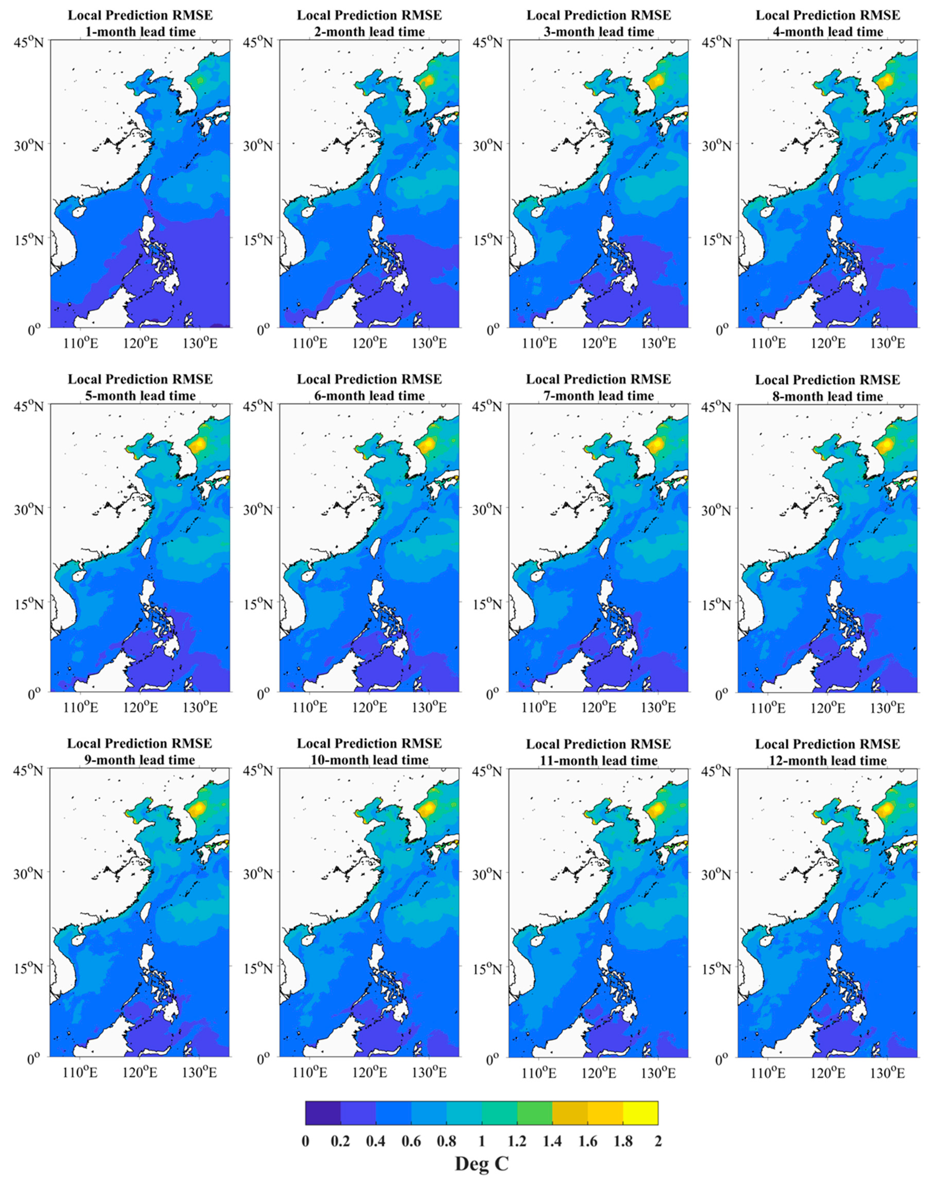
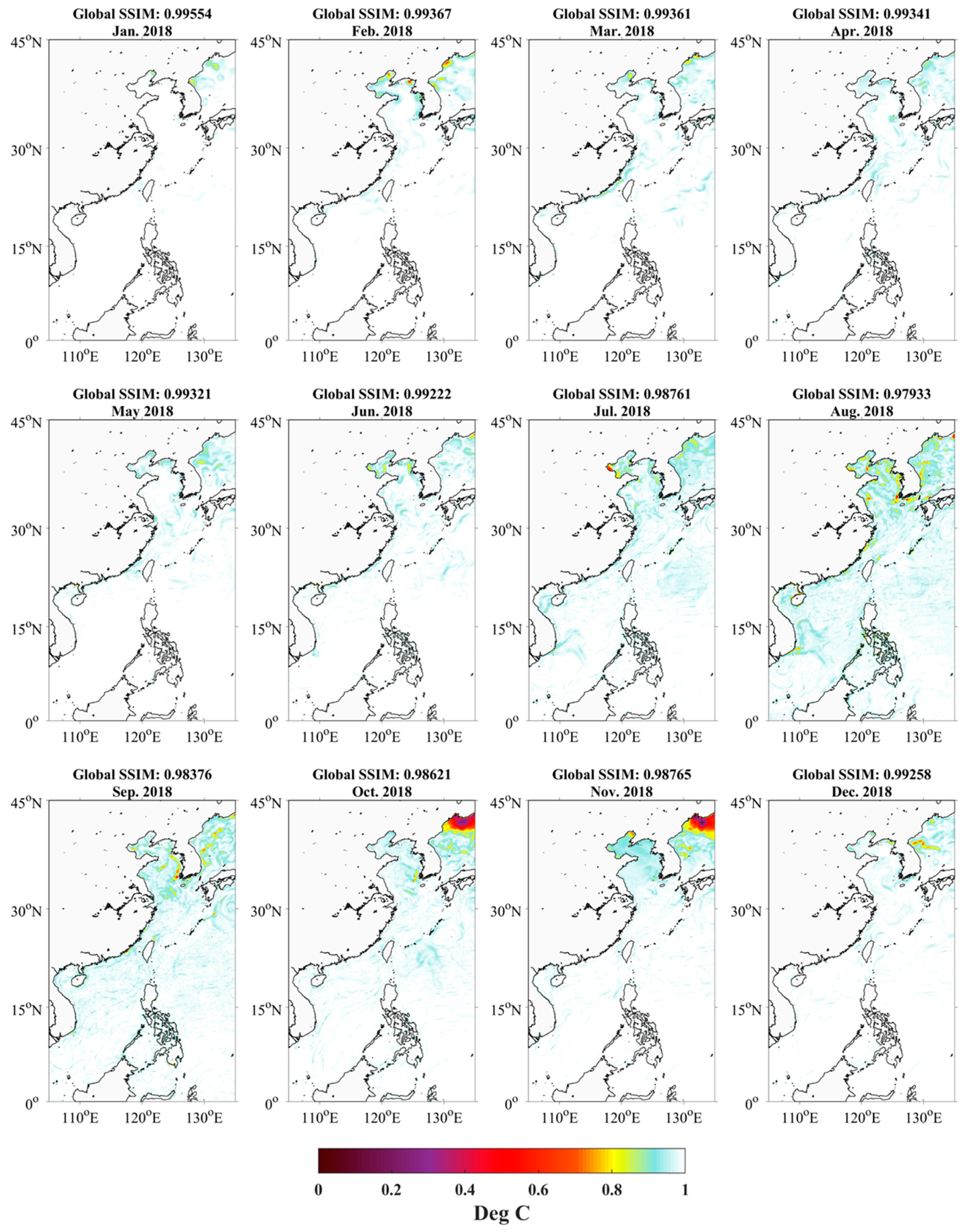
3.2. SST Prediction with Different Lead Times from 2015 to 2018

The monthly statistics including the biases and standard deviations as well as the average RMSE for the four years with different lead times using the proposed model are shown in Figure 11. The monthly biases and standard deviations obtained by the model are denoted by blue points and error bars. At a one-month lead time, the prediction accuracy is the highest, with the RMSE around 0.5 °C. When the lead time increases to two months, the RMSE increases to 0.59 °C and then slowly rises. It reaches a maximum when the lead time is 11 months, with an RMSE around 0.66 °C. Compared with the biases of each year, the standard deviations are more stable as the lead-time increases. Overall, the prediction error shows a fluctuating rising and falling tendency along with the prediction time series. Generally, a relatively large bias is likely to occur in summer, such as in August 2016. Compared with other months in 2016, the standard deviation of the prediction results for August suddenly increased. We checked the prediction results and found that the model underestimated the SST in the East China Sea more seriously. In the prediction period, the bias in 2015 is lower, which is –0.06 °C with a one-month lead time and –0.05 °C for a 12-month lead time.

Figure 12 shows the distribution of the RMSE from 2015 to 2018 with different prediction lead times in the study area. When the predicted lead time is gradually increased to 12 months, the RMSE near 0–10° N, 120–130° E is less than 0.4 °C; the RMSE near the eastern and southwestern Philippines, and near the Kuroshio is less than 0.6 °C; the RMSE near the coastal areas is around 1 °C. The prediction accuracy near the northeast of the Korean Peninsula is the lowest. Overall, from the southwest to the northeast of the study area, as the lead time increases, the prediction accuracy gradually decreases. The distribution patterns of prediction accuracy have a strong relationship with the ocean currents. The main current systems in the southeastern Taiwan area are the equatorial north flow and the Kuroshio mainstream. They are relatively stable in speed and temperature, generally with no regular seasonal changes. The prediction accuracy remains high under a long prediction lead time in this kind of area. The waters near the mainland are dominated by coastal currents. The direction of these currents changes seasonally. In some areas, e.g., the Yangtze River estuary and the northeast of the Korean Peninsula, the cold coastal currents join the warm currents, which means the water is characterized by large annual variations in temperature. The prediction accuracy noticeably decreases as the lead-time increases in the areas with large annual variations in temperature.

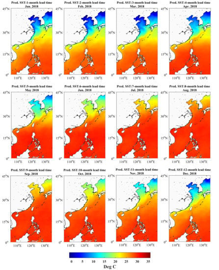
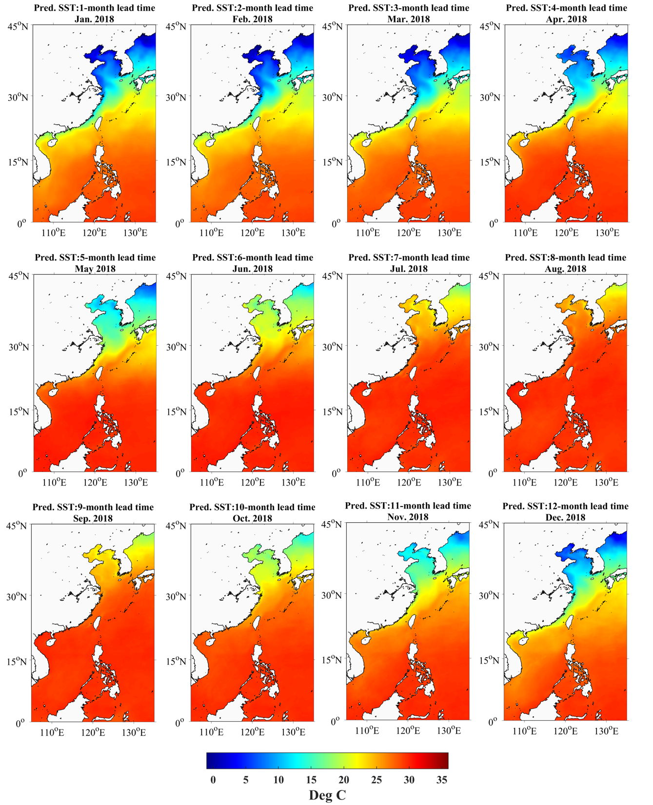
3.3. Predicted SST Distribution in Space

The 12-month distribution of predicted SSTs at 12 different lead times is shown in Figure 13. The SST features, like the Kuroshio, the Yellow Sea warm currents and the cold coastal China currents in winter are clearly shown in the prediction maps, and they show obvious seasonal variability. We adopted the SSIM [44] to evaluate the quality of the prediction maps relative to the validation maps. The local SSIM maps and global mean SSIM values are shown in Figure 14. Brighter pixels are associated with higher SSIM values, which means the SST patterns are more similar to the observed SST. This set of images shows that the predicted SST maps are overall consistent with those of the OSTIA SST maps. The global SSIM values are all above 0.97, and large pattern deviations mainly appear in the northern part of the Japan Sea, which means that the local SSIM is near 0.5. This suggests the classification of the study area does not affect the continuity of the SST pattern in this region. Figure 15 shows the differences in the SST distributions between the predicted results and the observation data. Most pixels’ values are within ±1 °C, and the percentages range from 85.17% to 98.19%, with the mean being 90.64% based on the statistics in

Table 1. Monthly statistics of SST differences in 2018.

2018	Jan.	Feb.	Mar.	Apr.	May	Jun.	Jul.	Aug.	Sep.	Oct.	Nov.	Dec.
Bias (°C)	0.05	0.28	0.06	0.26	−0.17	0.04	0.3	0.21	0.35	0.28	0.11	−0.29
SD (°C)	0.39	0.66	0.56	0.60	0.50	0.42	0.68	0.72	0.51	0.56	0.49	0.60
RMSE (°C)	0.39	0.71	0.56	0.65	0.53	0.42	0.74	0.75	0.62	0.63	0.50	0.67
P (±0.5 °C) %	84.09	55.06	68.93	58.5	75.78	81.23	57.53	48.56	55.74	66.52	72.82	57.30
P (±1 °C) %	98.19	87.53	93.47	86.86	93.36	96.92	85.17	85.46	88.63	90.57	95.53	85.95
P (±1.5 °C) %	99.59	96.34	98.3	98.07	97.72	99.60	94.00	95.03	99.35	96.87	98.84	97.68

. The predicted anomalies often occurred near the coastal area and the northern Japan Sea, which are beyond ±1 °C. In July and October, the area near 22° N, 130° E also has large biases. The possible reason may be related to the SST anomaly. As shown in Figure 16, the SST anomaly pattern obtained from OSTIA is similar to Figure 15. Generally, the areas with a large anomaly have a relatively low prediction accuracy. The biases, standard deviations, and RMSEs between the predicted and original OSTIA SST in 2018 were also calculated and are presented in Table 1. The biases range from −0.29 to 0.35 °C, with a mean of 0.12 °C; the standard deviations range from 0.39 to 0.72°C, with a mean of 0.56 °C.

4. Discussion

In the present study, we applied SOMs to classify the SST data, and then used the class labels obtained by the classification process as auxiliary inputs for LSTM-based model training and validation. Compared with the model trained without class labels, the prediction accuracy of the model trained with class labels was more stable and the bias was decreased. According to the China offshore ocean climate monitoring bulletin released by the National Marine Environment Forecasting Center, China offshore SST was generally higher than the same period of the previous year in July 2016 (a year with the strong El Niño) [45]. The model trained without class labels produced a wide range of underestimations in July, but the model trained with class labels reduced the bias considerably. The possible reason is that after classifying the SSTs in the study area through the SOM, the SSTs with different features are distinguished. These classification data containing regional information provide more characteristics during the model training process, which fits the data better and lowers the output bias.

The monthly statistical results with different prediction lead times showed that the prediction error had a fluctuating rising and falling tendency along with the prediction time series. The prediction SST had a large standard deviation in August 2016 compared with other months. We checked the error distribution and found that our model seriously underestimated the SST in the East China Sea. Referring to Tan and Cai [46], in 2018, the East China Seas experienced its warmest monthly mean SST. This extreme warming event was closely linked to the Indian Ocean Dipole (IOD). Since the SST of the Indian Ocean was not included in the training data set, the model had less capability to capture extreme warming. Another possible reason is that we used the IMS for multi-step prediction, which propagated errors from earlier time steps into later time steps, but we found no trend of linear error accumulation. Finally, the RMSE distribution in space suggested the prediction accuracy had a strong relationship with seasonal ocean current variability. Where the current was obvious and stable, the error was low; otherwise, the error obviously increased as the lead-time increased.

Overall, compared with the model trained without class labels, the prediction accuracy of the model trained with class labels was more stable and the bias was decreased in the periods with abnormally higher SST. The stable and accurate prediction may help to observe the SST trend and provide an outlook of climate change. However, the model still lacked the capability to predict extreme events. Therefore, in subsequent work, the IOD, monsoon, and current characteristics related to the SST changes in the study area will also be considered in model training. The spatial data around the sequence will also be added to improve the accuracy of long-term prediction.

5. Conclusions

In this study, we completed 12-month lead time SST predictions over the China Seas and their adjacent waters. The results had a RMSE of 0.5 °C with a one-month lead time and 0.66 °C with a 12-month lead time. The prediction accuracy was highest in the southeast of the study area, with an RMSE of less than 0.4 °C for a 12-month prediction lead time. This suggested it is feasible to place the data into a single model for spatio-temporal SST prediction. Introducing the spatial feature information through classification can improve prediction accuracy. Combining multiple models with different parameters and structures can improve the stability of prediction results.

References

1. Deser, C.; Phillips, A.S.; Alexander, M.A. Twentieth century tropical sea surface temperature trends revisited. Geophys. Res. Lett. 2010, 37. [Google Scholar] [CrossRef] [Green Version]
2. Alexander, M.A.; Scott, J.D.; Friedland, K.D.; Mills, K.E.; Nye, J.A.; Pershing, A.; Thomas, A.C. Projected sea surface temperatures over the 21st century: Changes in the mean, variability and extremes for large marine ecosystem regions of Northern Oceans. Elem. Sci. Anth. 2018, 6, 9. [Google Scholar] [CrossRef] [Green Version]
3. Tan, H.; Cai, R.; Huang, R. Enhanced Responses of Sea Surface Temperature over Offshore China to Global Warming and Hiatus. Clim. Chang. Res. 2016, 12, 500–507. [Google Scholar]
4. Wang, Q.; Li, Y.; Li, Q.; Liu, Y.; Wang, Y.-N. Changes in Means and Extreme Events of Sea Surface Temperature in the East China Seas Based on Satellite Data from 1982 to 2017. Atmosphere 2019, 10, 140. [Google Scholar] [CrossRef] [Green Version]
5. Cai, R.; Tan, H.; Kontoyiannis, H. Robust Surface Warming in Offshore China Seas and Its Relationship to the East Asian Monsoon Wind Field and Ocean Forcing on Interdecadal Time Scales. J. Clim. 2017, 30, 8987–9005. [Google Scholar] [CrossRef]
6. Liang, C.; Xian, W.; Pauly, D. Impacts of Ocean Warming on China’s Fisheries Catches: An Application of “Mean Temperature of the Catch” Concept. Front. Mar. Sci. 2018, 5, 5. [Google Scholar] [CrossRef] [Green Version]
7. Xu, G.; Lin, C. Relationship between the Variation of the Sea Surface Temperature over the South China Sea and the Rainfalls over the Middle and Lower Reaches of the Yangtze River in Jun. Sci. Meteorol. Sin. 1990, 10, 174–181. [Google Scholar]
8. McTaggart-Cowan, R.; Davies, E.L.; Fairman, J.G., Jr.; Galarneau, T.J., Jr.; Schultz, D.M. Revisiting the 26.5 °C sea surface temperature threshold for tropical cyclone development. Bull. Am. Meteorol. Soc. 2015, 96, 1929–1943. [Google Scholar] [CrossRef]
9. Ha, Y.; Zhong, Z.; Zhang, Y.; Ding, J.; Yang, X. Relationship between interannual changes of summer rainfall over Yangtze River Valley and South China Sea–Philippine Sea: Possible impact of tropical zonal sea surface temperature gradient. Int. J. Clim. 2019, 39, 5522–5538. [Google Scholar] [CrossRef] [Green Version]
10. Qiong, Z.; Ping, L.; Guoxiong, W. The relationship between the flood and drought over the lower reach of the Yangtze River valley and the SST over the Indian ocean and the South China Sea. Chin. J. Atmos. Sci. 2003, 27, 992–1006. [Google Scholar]
11. Liu, J.Y. Status of Marine Biodiversity of the China Seas. PLoS ONE 2013, 8, e50719. [Google Scholar] [CrossRef] [PubMed] [Green Version]
12. Thakur, K.; Vanderstichel, R.; Barrell, J.; Stryhn, H.; Patanasatienkul, T.; Revie, C.W. Comparison of Remotely-Sensed Sea Surface Temperature and Salinity Products With in Situ Measurements From British Columbia, Canada. Front. Mar. Sci. 2018, 5, 5. [Google Scholar] [CrossRef] [Green Version]
13. Fablet, R.; Viet, P.H.; Lguensat, R. Data-Driven Models for the Spatio-Temporal Interpolation of Satellite-Derived SST Fields. IEEE Trans. Comput. Imaging 2017, 3, 647–657. [Google Scholar] [CrossRef]
14. Tangang, F.T.; Hsieh, W.W.; Tang, B. Forecasting the equatorial Pacific sea surface temperatures by neural network models. Clim. Dyn. 1997, 13, 135–147. [Google Scholar] [CrossRef]
15. Tangang, F.T.; Hsieh, W.W.; Tang, B. Forecasting regional sea surface temperatures in the tropical Pacific by neural network models, with wind stress and sea level pressure as predictors. J. Geophys. Res. Space Phys. 1998, 103, 7511–7522. [Google Scholar] [CrossRef]
16. Tangang, F.T.; Tang, B.; Monahan, A.H.; Hsieh, W.W. Forecasting ENSO Events: A Neural Network–Extended EOF Approach. J. Clim. 1998, 11, 29–41. [Google Scholar] [CrossRef]
17. Wu, A.; Hsieh, W.W.; Tang, B. Neural network forecasts of the tropical Pacific sea surface temperatures. Neural Netw. 2006, 19, 145–154. [Google Scholar] [CrossRef] [Green Version]
18. Ali, M.M.; Weller, R.A.; Swain, D. Estimation of ocean subsurface thermal structure from surface parameters: A neural network approach. Geophys. Res. Lett. 2004, 31. [Google Scholar] [CrossRef] [Green Version]
19. Barrows, T.T.; Juggins, S. Sea-surface temperatures around the Australian margin and Indian Ocean during the Last Glacial Maximum. Quat. Sci. Rev. 2005, 24, 1017–1047. [Google Scholar] [CrossRef]
20. Hayes, A.; Kucera, M.; Kallel, N.; Sbaffi, L.; Rohling, E.J. Glacial Mediterranean sea surface temperatures based on planktonic foraminiferal assemblages. Quat. Sci. Rev. 2005, 24, 999–1016. [Google Scholar] [CrossRef]
21. Garcia-Gorriz, E.; Garcia-Sanchez, J. Prediction of sea surface temperatures in the western Mediterranean Sea by neural networks using satellite observations. Geophys. Res. Lett. 2007, 34. [Google Scholar] [CrossRef]
22. Patil, K.; Deo, M.C. Prediction of daily sea surface temperature using efficient neural networks. Ocean Dyn. 2017, 67, 357–368. [Google Scholar] [CrossRef]
23. Mahongo, S.B.; Deo, M.C. Using Artificial Neural Networks to Forecast Monthly and Seasonal Sea Surface Temperature Anomalies in the Western Indian Ocean. Int. J. Ocean Clim. Syst. 2013, 4, 133–150. [Google Scholar] [CrossRef] [Green Version]
24. Patil, K.; Deo, M.C.; Ravichandran, M. Prediction of Sea Surface Temperature by Combining Numerical and Neural Techniques. J. Atmos. Ocean. Technol. 2016, 33, 1715–1726. [Google Scholar] [CrossRef]
25. Wei, L.; Guan, L.; Qu, L. Prediction of Sea Surface Temperature in the South China Sea by Artificial Neural Networks. IEEE Geosci. Remote Sens. Lett. 2019, 17, 558–562. [Google Scholar] [CrossRef]
26. Zhang, Q.; Wang, H.; Dong, J.; Zhong, G.; Sun, X. Prediction of Sea Surface Temperature Using Long Short-Term Memory. IEEE Geosci. Remote Sens. Lett. 2017, 14, 1745–1749. [Google Scholar] [CrossRef] [Green Version]
27. Yang, Y.; Dong, J.; Sun, X.; Lima, E.; Mu, Q.; Wang, X. A CFCC-LSTM Model for Sea Surface Temperature Prediction. IEEE Geosci. Remote Sens. Lett. 2018, 15, 207–211. [Google Scholar] [CrossRef]
28. Patil, K.; Deo, M.C. Basin-Scale Prediction of Sea Surface Temperature with Artificial Neural Networks. J. Atmos. Ocean. Technol. 2018, 35, 1441–1455. [Google Scholar] [CrossRef]
29. Gong, S.; Wong, K. Spatio-Temporal Analysis of Sea Surface Temperature in the East China Sea Using TERRA/MODIS Products Data. In Sea Level Rise and Coastal Infrastructure; IntechOpen: London, UK, 2018. [Google Scholar]
30. Ouyang, L.; Hui, F.; Zhu, L.; Cheng, X.; Cheng, B.; Shokr, M.; Zhao, J.; Ding, M.; Zeng, T. The spatiotemporal patterns of sea ice in the Bohai Sea during the winter seasons of 2000–2016. Int. J. Digit. Earth 2019, 12, 893–909. [Google Scholar] [CrossRef]
31. Nihashi, S.; Ohshima, K.I.; Saitoh, S.-I. Sea-ice production in the northern Japan Sea. Deep. Sea Res. Part I Oceanogr. Res. Pap. 2017, 127, 65–76. [Google Scholar] [CrossRef]
32. Roberts-Jones, J.; Fiedler, E.K.; Martin, M.J. Daily, Global, High-Resolution SST and Sea Ice Reanalysis for 1985-2007 Using the Ostia System. J. Clim. 2012, 25, 6215–6231. [Google Scholar] [CrossRef]
33. McLaren, A.; Fiedler, E.; Roberts-Jones, J.; Martin, M.; Mao, C.; Good, S. Quality Information Document: Global Ocean OSTIA Near Real Time Level 4 Sea Surface Temperature Product. Available online: https://resources.marine.copernicus.eu/documents/QUID/CMEMS-OSI-QUID-010-001.pdf (accessed on 20 August 2020).
34. Kohonen, T.; Mäkisara, K. The self-organizing feature maps. Phys. Scr. 1989, 39, 168–172. [Google Scholar] [CrossRef]
35. Haykin, S. Neural Networks and Learning Machines; 3rd ed.; Pearson Education: Upper Saddle River, NJ, USA, 2009. [Google Scholar]
36. Oyana, T.J.; Achenie, L.E.; Cuadros-Vargas, E.; Rivers, P.A.; Scott, K.E. A Mathematical Improvement of the Self-Organizing Map Algorithm. In Proceedings from the International Conference on Advances in Engineering and Technology; Elsevier BV: Amsterdam, The Netherlands, 2006; pp. 522–531. [Google Scholar]
37. Hu, J.; Wang, X.H. Progress on upwelling studies in the China seas. Rev. Geophys. 2016, 54, 653–673. [Google Scholar] [CrossRef]
38. Hochreiter, S.; Schmidhuber, J. Long Short-Term Memory. Neural Comput. 1997, 9, 1735–1780. [Google Scholar] [CrossRef] [PubMed]
39. Fischer, T.; Krauss, C. Deep learning with long short-term memory networks for financial market predictions. Eur. J. Oper. Res. 2018, 270, 654–669. [Google Scholar] [CrossRef] [Green Version]
40. Olah, C. Understanding LSTM Networks. Available online: http://colah.github.io/posts/2015-08-Understanding-LSTMs/ (accessed on 8 March 2020).
41. Bengio, Y. Practical Recommendations for Gradient-Based Training of Neural Networks: Tricks of the Trade; Springer: Heidelberg, Germany, 2012; pp. 437–478. [Google Scholar]
42. Bergstra, J.; Bengio, Y. Random Search for Hyper-Parameter Optimization. J. Mach. Learn Res. 2012, 13, 281–305. [Google Scholar]
43. Bishop, C.M. Neural Networks for Pattern Recognition; Oxford University Press: New York, NY, USA, 1995. [Google Scholar]
44. Wang, Z.; Bovik, A.C.; Sheikh, H.R.; Simoncelli, E.P. Image quality assessment: From error visibility to structural similarity. IEEE Trans. Image Process. 2004, 13, 600–612. [Google Scholar] [CrossRef] [Green Version]
45. China Offshore Ocean Climate Monitoring Bulletin. Available online: http://www.nmefc.cn/chanpin/hyqh/qhjc/bulletin_201608.pdf (accessed on 1 July 2020).
46. Tan, H.; Cai, R. What caused the record-breaking warming in East China Seas during August 2016? Atmos. Sci. Lett. 2018, 19, e853. [Google Scholar] [CrossRef] [Green Version]
Figure 1. The major currents in the study area (the area within the blue dotted rectangle) [11].
Remotesensing 12 02697 g001
Figure 2. Data pre-processing workflow.
Remotesensing 12 02697 g002
Figure 3. Kohonen model architecture.
Remotesensing 12 02697 g003
Figure 4. Construction of the input and output vectors of the self-organizing feature map (SOM).
Remotesensing 12 02697 g004
Figure 5. The class map of the study area: (a) 5 classes; (b) 30 classes; (c) 60 classes; (d) 90 classes; (e) 110 classes; (f) 115 classes.
Remotesensing 12 02697 g005
Figure 6. Structure of long short-term memory (LSTM) memory cell [39,40].
Remotesensing 12 02697 g006
Figure 7. Construction of the input and target vectors of the LSTM model: (a) The model trained with class labels and (b) the model trained without class labels.
Remotesensing 12 02697 g007
Figure 8. The root mean square errors (RMSEs) with 12 steps prediction with different class label sets inputted under different ensemble members from 2015 to 2018.
Remotesensing 12 02697 g008
Figure 9. Yearly statistics of the SST difference from the model trained with class labels (blue bars) and without class labels (red bars) from 2015 to 2018.
Remotesensing 12 02697 g009
Figure 10. The SST differences distribution in 2016. (a) The model trained with class labels; (b) the model trained without class labels.
Remotesensing 12 02697 g010
Figure 11. Monthly statistics from 2015 to 2018.
Remotesensing 12 02697 g011
Figure 12. The RMSE of prediction results distribution.
Remotesensing 12 02697 g012
Figure 13. SST distribution in 2018.
Remotesensing 12 02697 g013
Figure 14. Local structural similarity index (SSIM) maps in 2018.
Remotesensing 12 02697 g014
Figure 15. SST difference between the predicted SST and Operational SST and Ice Analysis (OSTIA) SST in 2018.
Remotesensing 12 02697 g015
Figure 16. SST anomaly in 2018.
Remotesensing 12 02697 g016