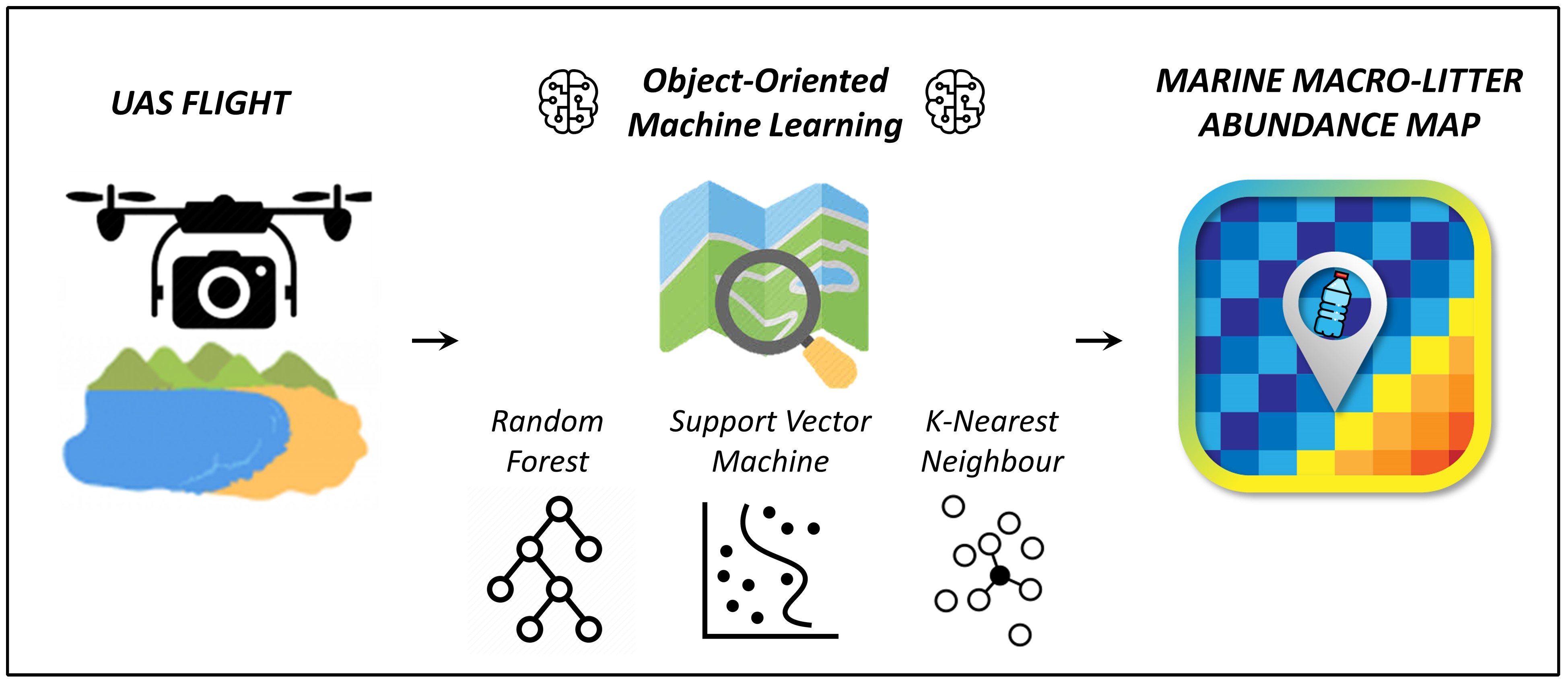
Quantifying Marine Macro Litter Abundance on a Sandy Beach Using Unmanned Aerial Systems and Object-Oriented Machine Learning Methods


Abstract

1. Introduction
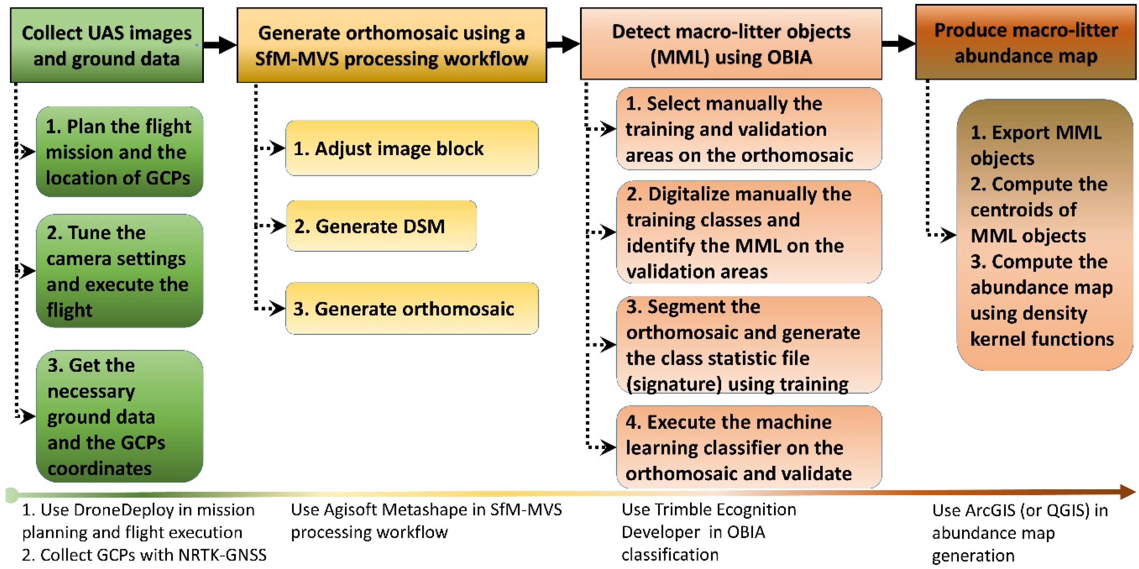
2. Materials and Methods
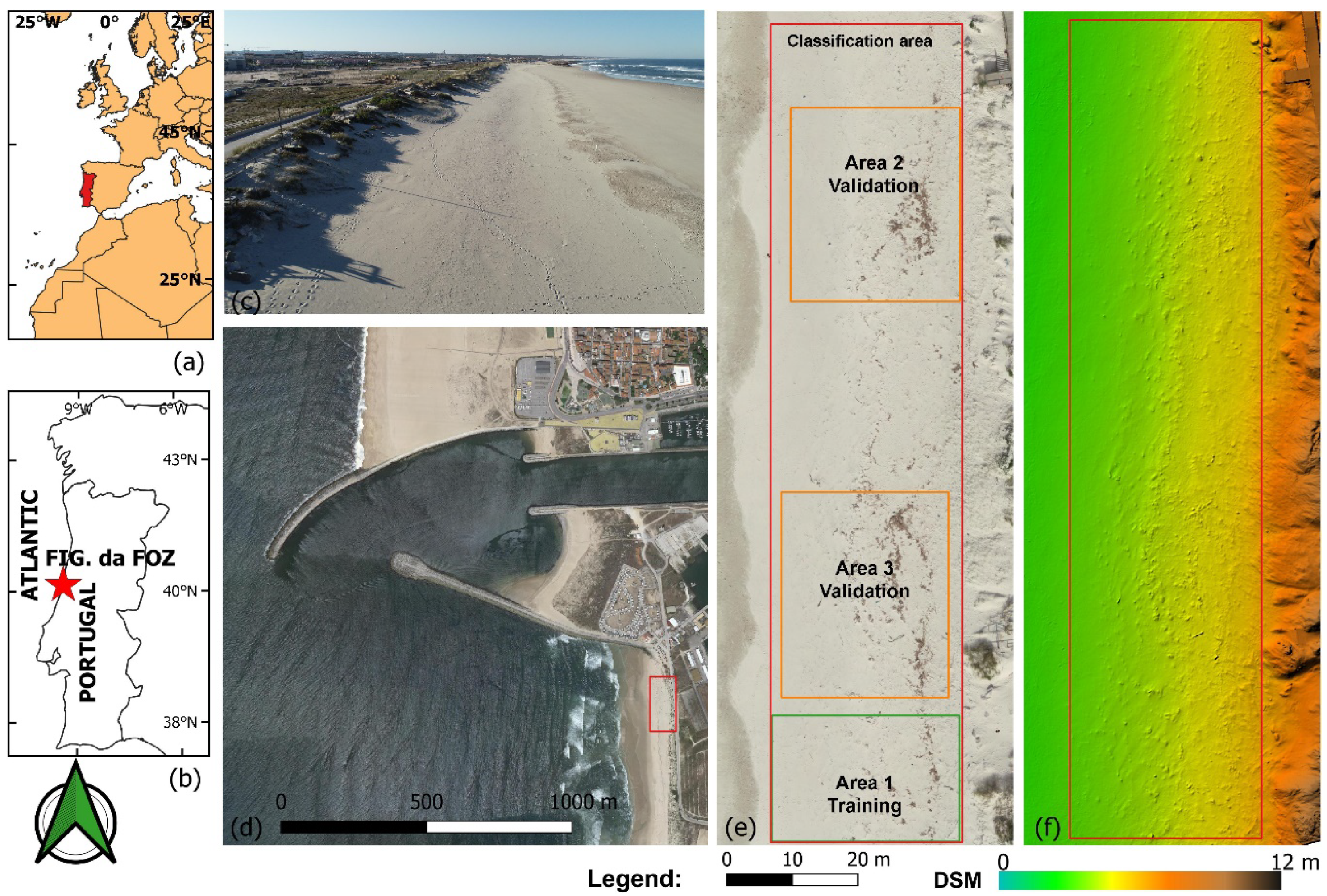
2.1. Study Area
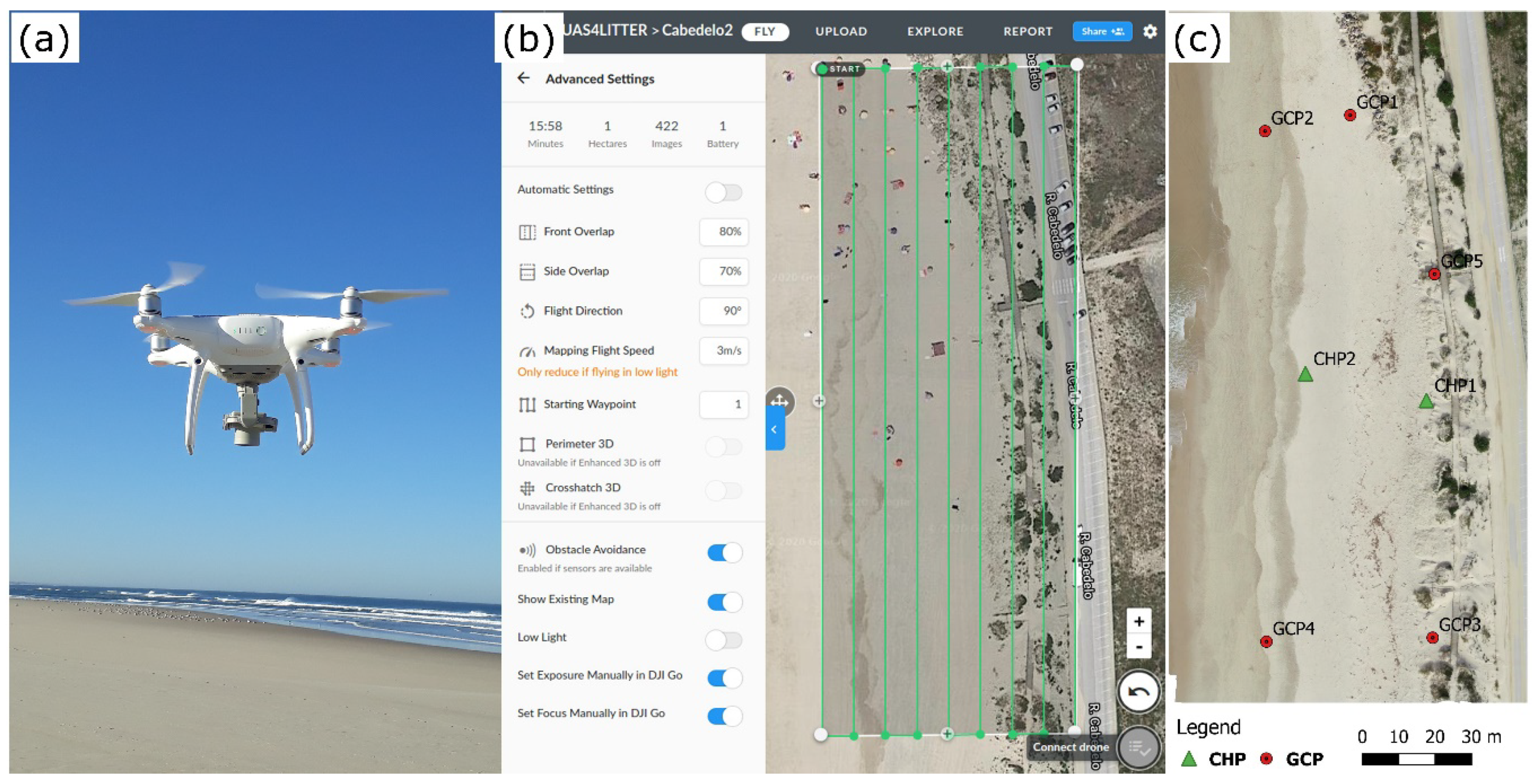
2.2. Field Data Acquisition and Unmanned Aerial Syetem (UAS) Survey
2.3. Structure from Motion and Multi Video Stereo (SfM-MVS) Processing
- Photo alignment Using the keypoints detected on each image, the process computes the internal camera parameters (e.g., lens distortion), the external orientation parameters for each image, and generates a sparse 3D point cloud.
- Georeferencing The geospatial 3D point cloud is assigned to a specific cartographic (or geographic) coordinate system.
- Camera optimization Camera calibration and the estimation of its interior orientation parameters are refined by an optimization procedure, which minimizes the sum of re-projection errors and reference coordinate misalignments. For this step, the sparse point cloud is statistically analyzed to delete misallocated points and to find the optimal re-projection solution.
- Dense matching The MVS dense matching technique generates a 3D dense point cloud from multiple images with optimized internal and external orientation parameters.
- DSM and orthomosaic generation The DSM is interpolated from the 3D dense point cloud, and consequently, the orthomosaic is generated from this DSM. It is worthwhile to note that we imaged a scene with low variation in height relative to the flying height. Therefore, the extra time-consuming steps of mesh generation and 3D texture mapping were not necessary for the generation of the orthomosaic.
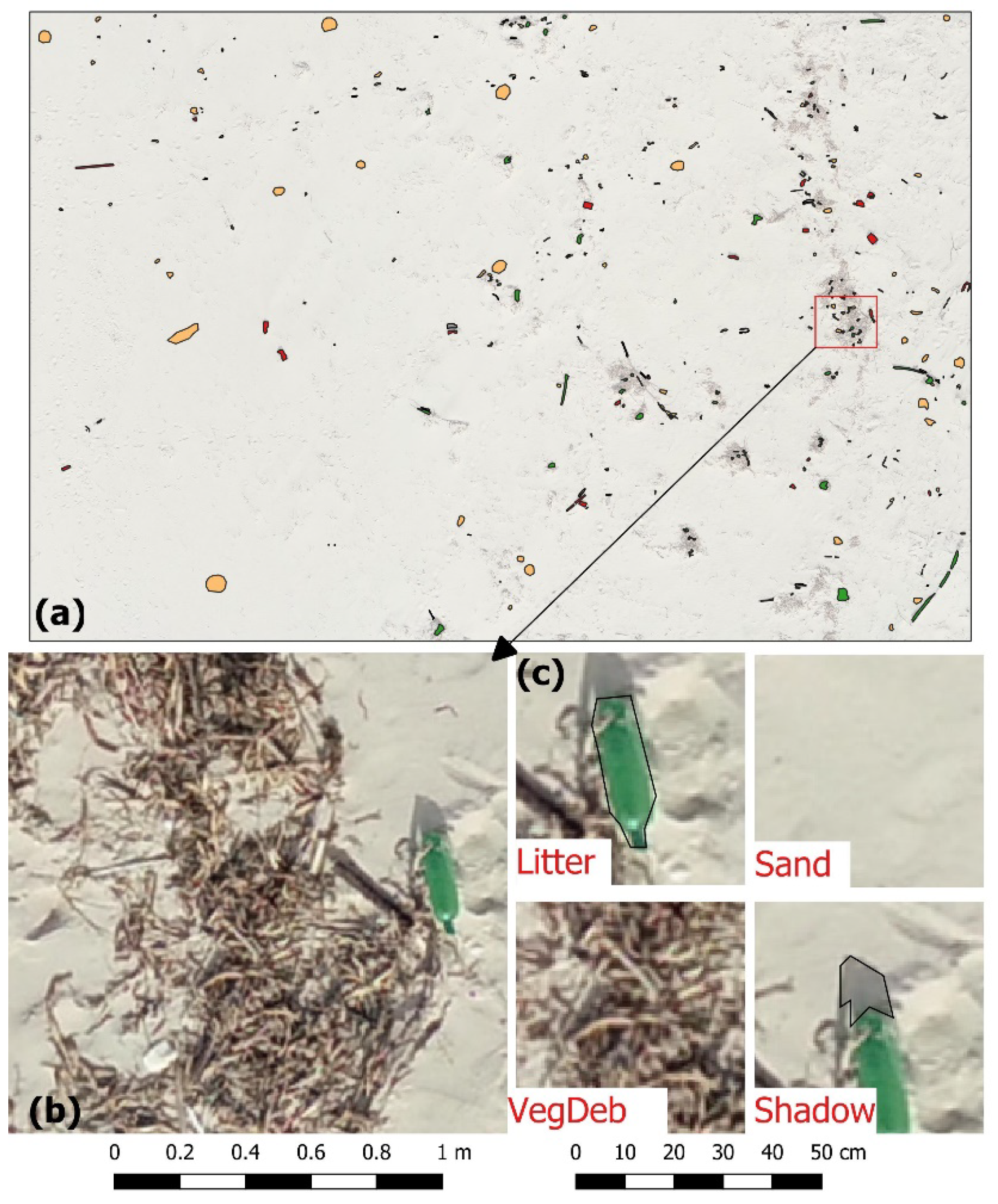
2.4. Classification Preprocessing, Nomenclature, and Training Areas
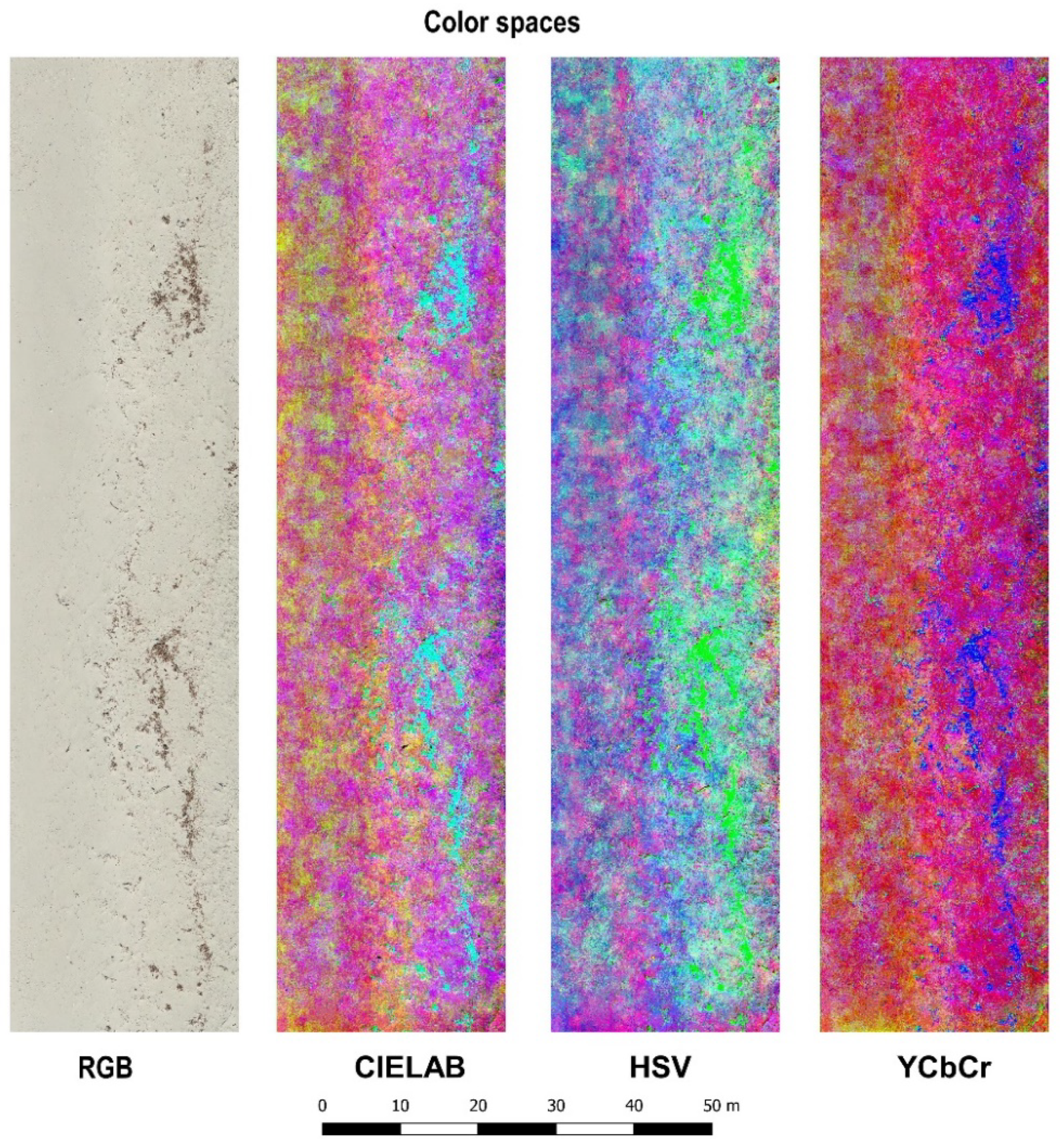
2.5. Feature Space and Data Normalization
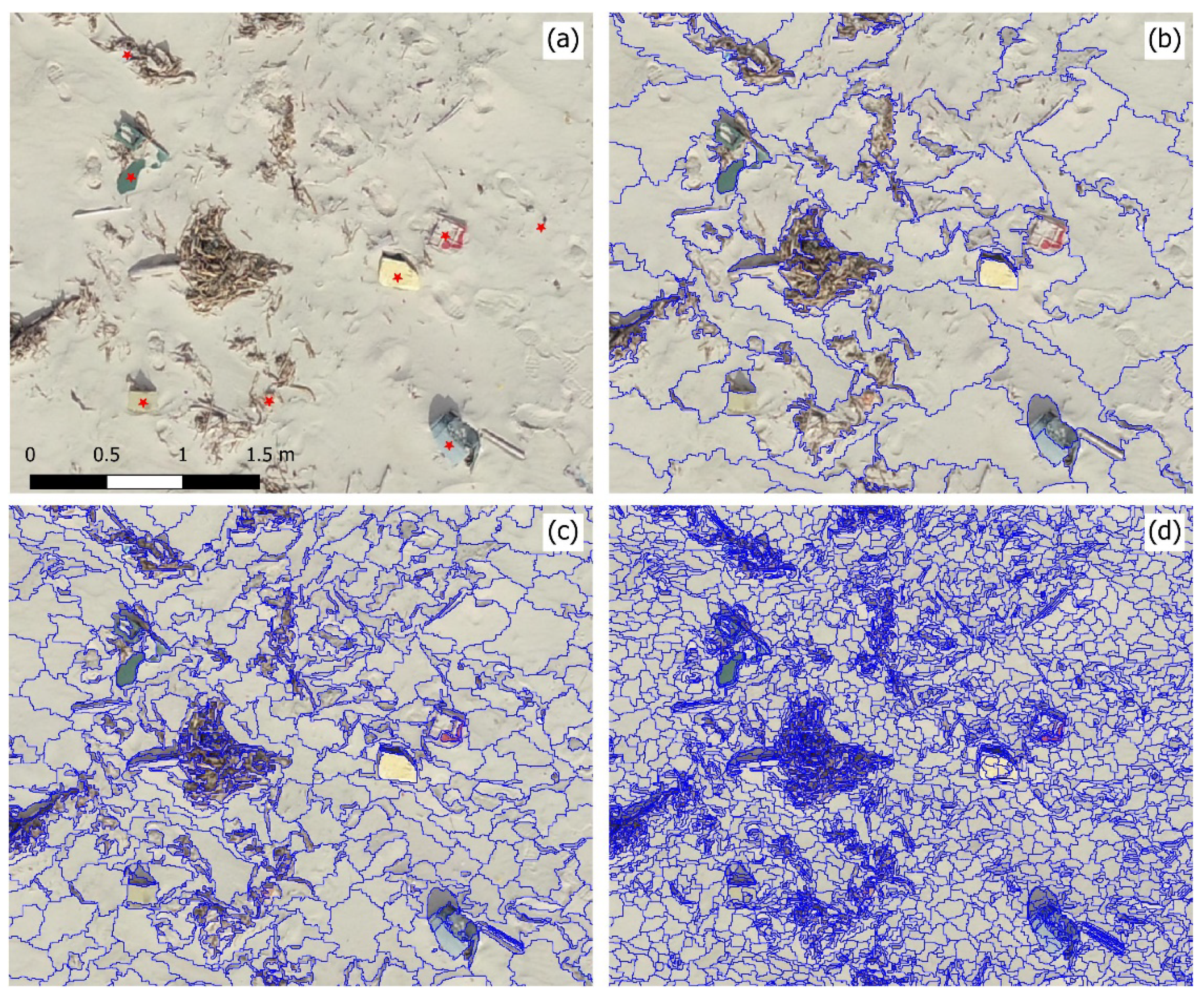
2.6. Image Segmentation
2.7. Classifiers and User-Defined Parameters
2.7.1. Random Forest
2.7.2. Support Vector Machine
2.7.3. K-Nearest Neighbor
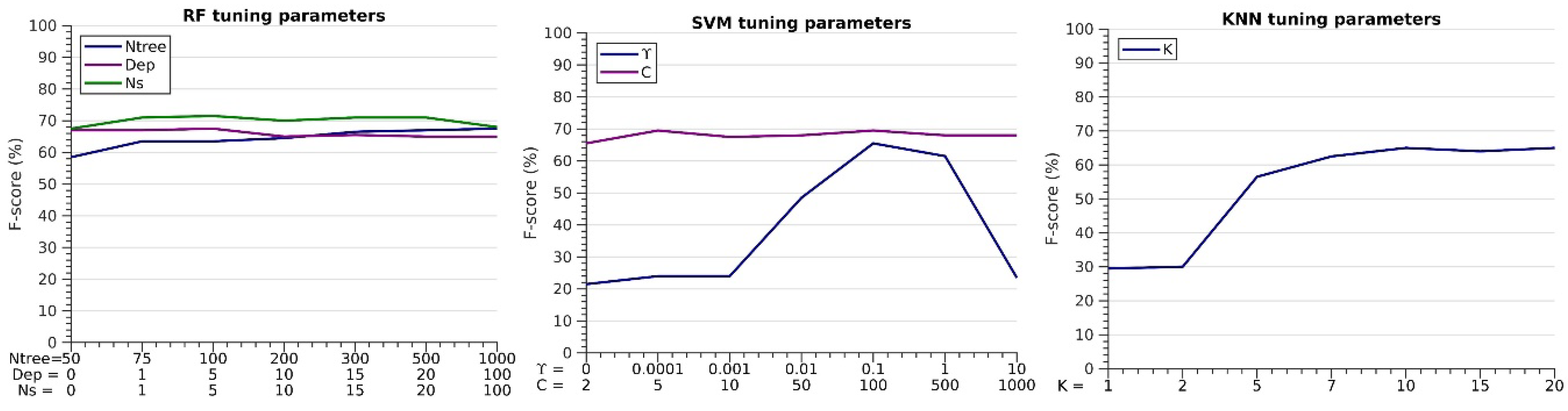
2.8. Tuning the Primary Classifier Parameters
2.9. Performance Assessment
2.10. Quantifying Macro Litter Abundance
3. Results
3.1. Georeferencing Accuracy
3.2. Effects of the Tuning Parameters on the F-Score
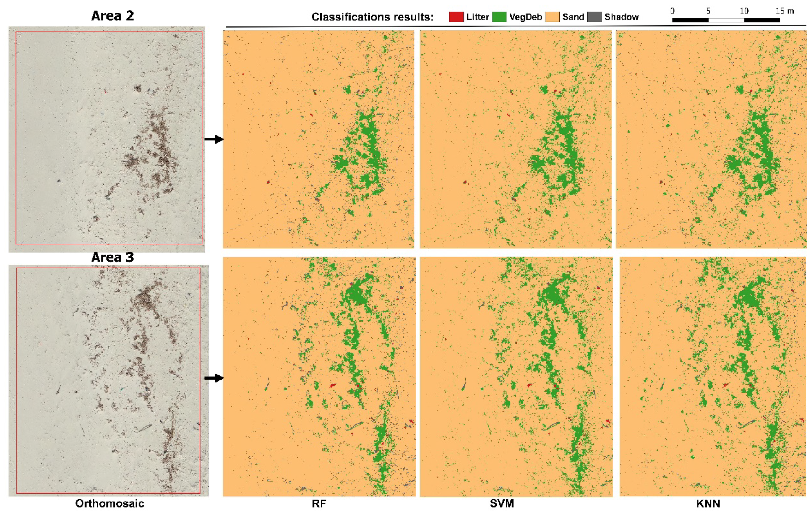
3.3. Comparisons of the Classifiers for Mapping Marine Litter
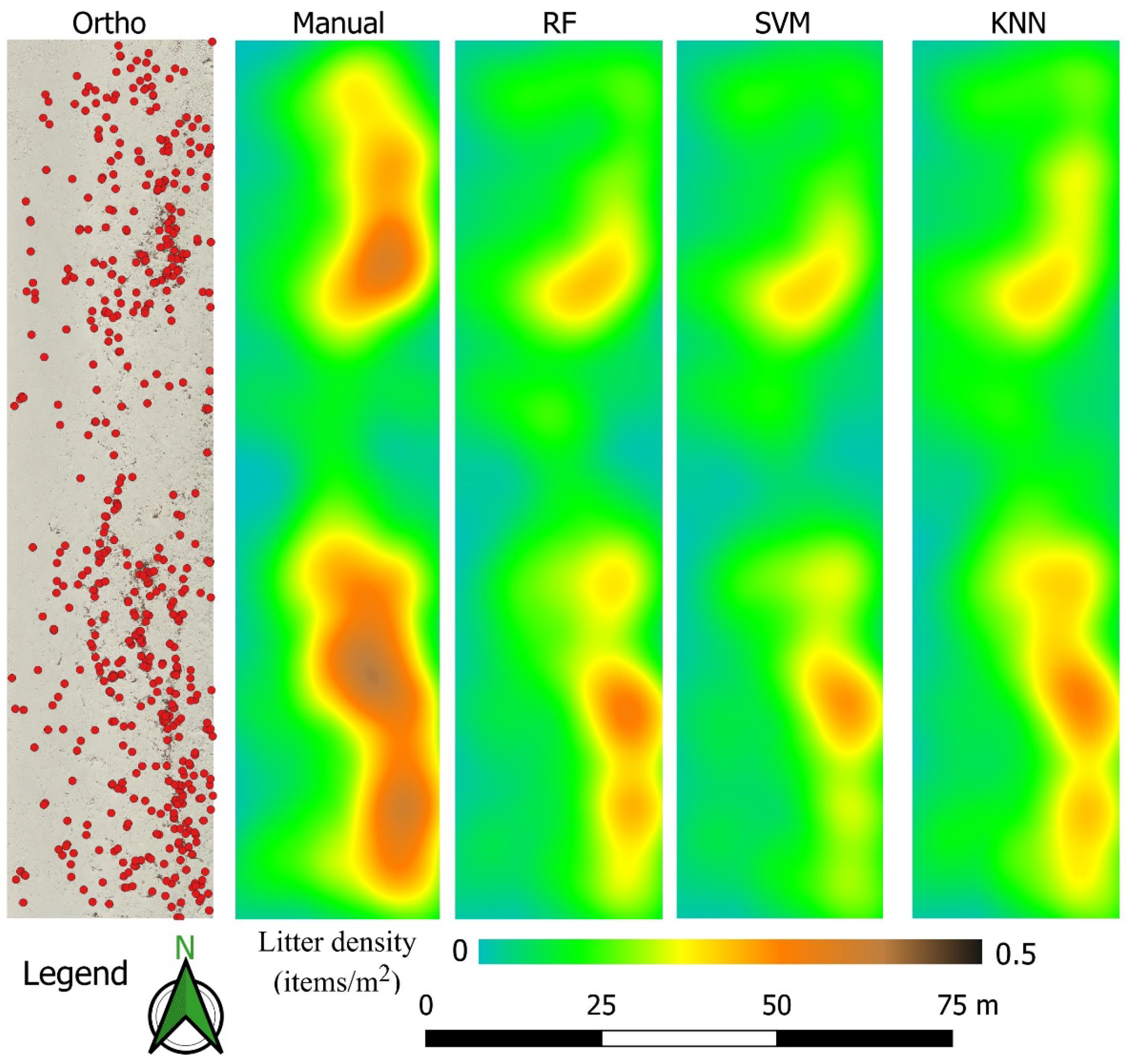
3.4. Mapping Marine Litter Abundance
4. Discussion
4.1. UAS Type and Flight Mission
4.2. Object-Oriented Machine Learning Methods
5. Conclusions
Author Contributions
Funding
Conflicts of Interest
References
- Fleming, L.E.; Broad, K.; Clement, A.; Dewailly, E.; Elmir, S.; Knap, A.; Pomponi, S.A.; Smith, S.; Solo Gabriele, H.; Walsh, P. Oceans and human health: Emerging public health risks in the marine environment. Mar. Pollut. Bull. 2006, 53, 545–560. [Google Scholar] [CrossRef] [PubMed]
- Galgani, F.; Hanke, G.; Maes, T. Global distribution, composition and abundance of marine litter. In Marine Anthropogenic Litter; Springer: Cham, Switzerland, 2015; ISBN 9783319165103. [Google Scholar]
- Veiga, J.M.; Fleet, D.; Kinsey, S.; Nilsson, P.; Vlachogianni, T.; Werner, S.; Galgani, F.; Thompson, R.C.; Dagevos, J.; Gago, J.; et al. Identifying Sources of Marine Litter. MSFD GES TG Marine Litter Thematic Report; Publications Office of the European Union: Luxembourg, 2016; ISBN 9789279645228. [Google Scholar]
- Ogunola, O.S.; Onada, O.A.; Falaye, A.E. Mitigation measures to avert the impacts of plastics and microplastics in the marine environment (a review). Environ. Sci. Pollut. Res. 2018, 25, 9293–9310. [Google Scholar] [CrossRef] [PubMed]
- Munari, C.; Corbau, C.; Simeoni, U.; Mistri, M. Marine litter on Mediterranean shores: Analysis of composition, spatial distribution and sources in north-western Adriatic beaches. Waste Manag. 2016, 49, 483–490. [Google Scholar] [CrossRef] [PubMed]
- Ríos, N.; Frias, J.P.G.L.; Rodríguez, Y.; Carriço, R.; Garcia, S.M.; Juliano, M.; Pham, C.K. Spatio-temporal variability of beached macro-litter on remote islands of the North Atlantic. Mar. Pollut. Bull. 2018, 133, 304–311. [Google Scholar] [CrossRef] [PubMed]
- Galgani, F. Marine litter, future prospects for research. Front. Mar. Sci. 2015, 2, 1–5. [Google Scholar] [CrossRef]
- Schulz, M.; Clemens, T.; Förster, H.; Harder, T.; Fleet, D.; Gaus, S.; Grave, C.; Flegel, I.; Schrey, E.; Hartwig, E. Statistical analyses of the results of 25 years of beach litter surveys on the south-eastern North Sea coast. Mar. Environ. Res. 2015, 109, 21–27. [Google Scholar] [CrossRef]
- Schulz, M.; van Loon, W.; Fleet, D.M.; Baggelaar, P.; van der Meulen, E. OSPAR standard method and software for statistical analysis of beach litter data. Mar. Pollut. Bull. 2017, 122, 166–175. [Google Scholar] [CrossRef]
- Oigman-Pszczol, S.S.; Creed, J.C. Quantification and Classification of Marine Litter on Beaches along Armação dos Búzios, Rio de Janeiro, Brazil. J. Coast. Res. 2007, 232, 421–428. [Google Scholar] [CrossRef]
- Kusui, T.; Noda, M. International survey on the distribution of stranded and buried litter on beaches along the Sea of Japan. Mar. Pollut. Bull. 2003, 47, 175–179. [Google Scholar] [CrossRef]
- Zhou, P.; Huang, C.; Fang, H.; Cai, W.; Li, D.; Li, X.; Yu, H. The abundance, composition and sources of marine debris in coastal seawaters or beaches around the northern South China Sea (China). Mar. Pollut. Bull. 2011, 62, 1998–2007. [Google Scholar] [CrossRef]
- Hong, S.; Lee, J.; Kang, D.; Choi, H.W.; Ko, S.H. Quantities, composition, and sources of beach debris in Korea from the results of nationwide monitoring. Mar. Pollut. Bull. 2014, 84, 27–34. [Google Scholar] [CrossRef] [PubMed]
- Prevenios, M.; Zeri, C.; Tsangaris, C.; Liubartseva, S.; Fakiris, E.; Papatheodorou, G. Beach litter dynamics on Mediterranean coasts: Distinguishing sources and pathways. Mar. Pollut. Bull. 2018, 129, 448–457. [Google Scholar] [CrossRef] [PubMed]
- Williams, A.T.; Randerson, P.; Di Giacomo, C.; Anfuso, G.; Macias, A.; Perales, J.A. Distribution of beach litter along the coastline of Cádiz, Spain. Mar. Pollut. Bull. 2016, 107, 77–87. [Google Scholar] [CrossRef] [PubMed]
- Frias, J.P.G.L.; Antunes, J.C.; Sobral, P. Local marine litter survey—A case study in Alcobaça municipality, Portugal. Rev. Gestão Costeira Integr. 2013, 13, 169–179. [Google Scholar] [CrossRef]
- Eriksson, C.; Burton, H.; Fitch, S.; Schulz, M.; van den Hoff, J. Daily accumulation rates of marine debris on sub-Antarctic island beaches. Mar. Pollut. Bull. 2013, 66, 199–208. [Google Scholar] [CrossRef]
- Storrier, K.L.; McGlashan, D.J. Development and management of a coastal litter campaign: The voluntary coastal partnership approach. Mar. Policy 2006, 30, 189–196. [Google Scholar] [CrossRef]
- Rees, G.; Pond, K. Marine litter monitoring programmes—A review of methods with special reference to national surveys. Mar. Pollut. Bull. 1995, 30, 103–108. [Google Scholar] [CrossRef]
- Haseler, M.; Schernewski, G.; Balciunas, A.; Sabaliauskaite, V. Monitoring methods for large micro- and meso-litter and applications at Baltic beaches. J. Coast. Conserv. 2018, 22, 27–50. [Google Scholar] [CrossRef]
- GESAMP. Guidelines for the Monitoring and Assessment of Plastic Litter in the Ocean; GESAMP Joint Group of Experts on the Scientific Aspects of Marine Environmental Protection: London, UK, 2019. [Google Scholar]
- Fallati, L.; Polidori, A.; Salvatore, C.; Saponari, L.; Savini, A.; Galli, P. Anthropogenic Marine Debris assessment with Unmanned Aerial Vehicle imagery and deep learning: A case study along the beaches of the Republic of Maldives. Sci. Total Environ. 2019, 693, 133581. [Google Scholar] [CrossRef]
- Martin, C.; Parkes, S.; Zhang, Q.; Zhang, X.; McCabe, M.F.; Duarte, C.M. Use of unmanned aerial vehicles for efficient beach litter monitoring. Mar. Pollut. Bull. 2018, 131, 662–673. [Google Scholar] [CrossRef]
- Bao, Z.; Sha, J.; Li, X.; Hanchiso, T.; Shifaw, E. Monitoring of beach litter by automatic interpretation of unmanned aerial vehicle images using the segmentation threshold method. Mar. Pollut. Bull. 2018, 137, 388–398. [Google Scholar] [CrossRef] [PubMed]
- Deidun, A.; Gauci, A.; Lagorio, S.; Galgani, F. Optimising beached litter monitoring protocols through aerial imagery. Mar. Pollut. Bull. 2018, 131, 212–217. [Google Scholar] [CrossRef] [PubMed]
- Gonçalves, G.; Andriolo, U.; Pinto, L.; Duarte, D. Mapping marine litter with Unmanned Aerial Systems: A showcase comparison among manual image screening and machine learning techniques. Mar. Pollut. Bull. 2020, 155, 111158. [Google Scholar] [CrossRef]
- Gonçalves, G.; Andriolo, U.; Pinto, L.; Bessa, F. Mapping marine litter using UAS on a beach-dune system: A multidisciplinary approach. Sci. Total Environ. 2020, 706, 135742. [Google Scholar] [CrossRef] [PubMed]
- Andriolo, U.; Gonçalves, G.; Bessa, F.; Sobral, P. Mapping marine litter on coastal dunes with unmanned aerial systems: A showcase on the Atlantic Coast. Sci. Total Environ. 2020, 736, 139632. [Google Scholar] [CrossRef]
- Merlino, S.; Paterni, M.; Berton, A.; Massetti, L. Unmanned Aerial Vehicles for Debris Survey in Coastal Areas: Long-Term Monitoring Programme to Study Spatial and Temporal Accumulation of the Dynamics of Beached Marine Litter. Remote Sens. 2020, 12, 1260. [Google Scholar] [CrossRef]
- Publications Office of the EU. Guidance on Monitoring of Marine Litter in European Seas. Available online: https://op.europa.eu/en/publication-detail/-/publication/76da424f-8144-45c6-9c5b-78c6a5f69c5d/language-en (accessed on 16 July 2020).
- Lo, H.S.; Wong, L.C.; Kwok, S.H.; Lee, Y.K.; Po, B.H.K.; Wong, C.Y.; Tam, N.F.Y.; Cheung, S.G. Field test of beach litter assessment by commercial aerial drone. Mar. Pollut. Bull. 2020, 151, 110823. [Google Scholar] [CrossRef]
- Kataoka, T.; Hinata, H.; Kako, S. A new technique for detecting colored macro plastic debris on beaches using webcam images and CIELUV. Mar. Pollut. Bull. 2012, 64, 1829–1836. [Google Scholar] [CrossRef]
- Blaschke, T. Object based image analysis for remote sensing. ISPRS J. Photogramm. Remote Sens. 2010, 65, 2–16. [Google Scholar] [CrossRef]
- OSPAR Commission. Guideline for Monitoring Marine Litter on the Beaches in the OSPAR Maritime Area; OSPAR Commission: London, UK, 2010; Volume 1. [Google Scholar]
- Gašparović, M.; Jurjević, L. Gimbal influence on the stability of exterior orientation parameters of UAV acquired images. Sensors 2017, 17, 401. [Google Scholar] [CrossRef]
- Tmušić, G.; Manfreda, S.; Aasen, H.; James, M.R.; Gonçalves, G.; Ben-Dor, E.; Brook, A.; Polinova, M.; Arranz, J.J.; Mészáros, J.; et al. Current Practices in UAS-based Environmental Monitoring. Remote Sens. 2020, 12, 1001. [Google Scholar] [CrossRef]
- O’Connor, J.; Smith, M.J.; James, M.R. Cameras and settings for aerial surveys in the geosciences. Prog. Phys. Geogr. 2017, 41, 325–344. [Google Scholar] [CrossRef]
- Eltner, A.; Sofia, G. Structure from motion photogrammetric technique. Dev. Earth Surf. Process. 2020, 23, 1–24. [Google Scholar]
- Smith, M.W.; Carrivick, J.L.; Quincey, D.J. Structure from motion photogrammetry in physical geography. Prog. Phys. Geogr. 2015, 40, 247–275. [Google Scholar] [CrossRef]
- Agisoft LLC. Agisoft Metashape User Manual; Version 1.5; Agisoft LLC: Saint Petersburg, Russia, 2019. [Google Scholar]
- Jensen, J.R. Introductory Digital Image Processing: A Remote Sensing Perspective, 4th ed.; Prentince Hall: Upper Saddle River, NJ, USA, 2005; ISBN 9780134058160. [Google Scholar]
- Duro, D.C.; Franklin, S.E.; Dubé, M.G. A comparison of pixel-based and object-based image analysis with selected machine learning algorithms for the classification of agricultural landscapes using SPOT-5 HRG imagery. Remote Sens. Environ. 2012, 118, 259–272. [Google Scholar] [CrossRef]
- Belgiu, M.; Drăgu, L. Random forest in remote sensing: A review of applications and future directions. ISPRS J. Photogramm. Remote Sens. 2016, 114, 24–31. [Google Scholar] [CrossRef]
- Lu, D.; Weng, Q. A survey of image classification methods and techniques for improving classification performance. Int. J. Remote Sens. 2007, 28, 823–870. [Google Scholar] [CrossRef]
- Shaik, K.B.; Ganesan, P.; Kalist, V.; Sathish, B.S.; Jenitha, J.M.M. Comparative Study of Skin Color Detection and Segmentation in HSV and YCbCr Color Space. Procedia Comput. Sci. 2015, 57, 41–48. [Google Scholar] [CrossRef]
- Fairchild, M.D. Color Appearance Models; John Wiley & Sons, Ltd.: Chichester, UK, 2013; ISBN 9781118653128. [Google Scholar]
- Drǎguţ, L.; Tiede, D.; Levick, S.R. ESP: A tool to estimate scale parameter for multiresolution image segmentation of remotely sensed data. Int. J. Geogr. Inf. Sci. 2010, 24, 859–871. [Google Scholar] [CrossRef]
- Huang, H.; Lan, Y.; Yang, A.; Zhang, Y.; Wen, S.; Deng, J. Deep learning versus Object-based Image Analysis (OBIA) in weed mapping of UAV imagery. Int. J. Remote Sens. 2020, 41, 3446–3479. [Google Scholar] [CrossRef]
- Trimble. eCognition Developer: User Guide; Trimble: Munich, Germany, 2019. [Google Scholar]
- Laliberte, A.S.; Rango, A. Texture and scale in object-based analysis of subdecimeter resolution unmanned aerial vehicle (UAV) imagery. IEEE Trans. Geosci. Remote Sens. 2009, 47, 1–10. [Google Scholar] [CrossRef]
- Breiman, L. Random forests. Mach. Learn. 2001, 45, 5–32. [Google Scholar] [CrossRef]
- Maxwell, A.E.; Warner, T.A.; Fang, F. Implementation of machine-learning classification in remote sensing: An applied review. Int. J. Remote Sens. 2018, 39, 2784–2817. [Google Scholar] [CrossRef]
- Ghosh, A.; Joshi, P.K. A comparison of selected classification algorithms for mappingbamboo patches in lower Gangetic plains using very high resolution WorldView 2 imagery. Int. J. Appl. Earth Obs. Geoinf. 2014, 26, 298–311. [Google Scholar] [CrossRef]
- Mountrakis, G.; Im, J.; Ogole, C. Support vector machines in remote sensing: A review. ISPRS J. Photogramm. Remote Sens. 2011, 66, 247–259. [Google Scholar] [CrossRef]
- Qian, Y.; Zhou, W.; Yan, J.; Li, W.; Han, L. Comparing machine learning classifiers for object-based land cover classification using very high resolution imagery. Remote Sens. 2015, 7, 153–168. [Google Scholar] [CrossRef]
- Pal, M. Random forest classifier for remote sensing classification. Int. J. Remote Sens. 2005, 26, 217–222. [Google Scholar] [CrossRef]
- Mather, P.; Tso, B. Classification Methods for Remotely Sensed Data; CRC Press: Boca Raton, FL, USA, 2016; ISBN 9780429192029. [Google Scholar]
- Chirici, G.; Mura, M.; McInerney, D.; Py, N.; Tomppo, E.O.; Waser, L.T.; Travaglini, D.; McRoberts, R.E. A meta-analysis and review of the literature on the k-Nearest Neighbors technique for forestry applications that use remotely sensed data. Remote Sens. Environ. 2016, 176, 282–294. [Google Scholar] [CrossRef]
- González-Ramiro, A.; Gonçalves, G.; Sanchez-Rios, A.; Jeong, J.S. Using a VGI and GIS-based multicriteria approach for assessing the potential of rural tourism in Extremadura (Spain). Sustainability 2016, 8, 1144. [Google Scholar] [CrossRef]
- Fotheringham, S.; Brundson, C.; Chalrton, M. Qualitative Geography: Perspectives on Spatial Data Analysis; SAGE Publications: London, UK, 2010; ISBN 9780761959472. [Google Scholar]
- Przybilla, H.; Bäumker, M. RTK and PPK: GNSS-Technologies for direct georeferencing of UAV image flights (10801). In Proceedings of the FIG Working Week 2020 Smart Surveyors for Land and Water Management, Amsterdam, The Netherlands, 10–14 May 2020; pp. 10–14. [Google Scholar]
- Kako, S.; Isobe, A.; Magome, S. Low altitude remote-sensing method to monitor marine and beach litter of various colors using a balloon equipped with a digital camera. Mar. Pollut. Bull. 2012, 64, 1156–1162. [Google Scholar] [CrossRef]
- Kako, S.; Morita, S.; Taneda, T. Estimation of plastic marine debris volumes on beaches using unmanned aerial vehicles and image processing based on deep learning. Mar. Pollut. Bull. 2020, 155, 111127. [Google Scholar] [CrossRef] [PubMed]
- Kedzierski, M.; Wierzbicki, D.; Sekrecka, A.; Fryskowska, A.; Walczykowski, P.; Siewert, J. Influence of lower atmosphere on the radiometric quality of unmanned aerial vehicle imagery. Remote Sens. 2019, 11, 1214. [Google Scholar] [CrossRef]
- Acuña-Ruz, T.; Uribe, D.; Taylor, R.; Amézquita, L.; Guzmán, M.C.; Merrill, J.; Martínez, P.; Voisin, L.; Mattar, B.C. Anthropogenic marine debris over beaches: Spectral characterization for remote sensing applications. Remote Sens. Environ. 2018, 217, 309–322. [Google Scholar] [CrossRef]
- Mack, B.; Roscher, R.; Waske, B. Can I Trust My One-Class Classification? Remote Sens. 2014, 6, 8779–8802. [Google Scholar] [CrossRef]
- Deng, X.; Li, W.; Liu, X.; Guo, Q.; Newsam, S. One-class remote sensing classification: One-class vs. Binary classifiers. Int. J. Remote Sens. 2018, 39, 1890–1910. [Google Scholar] [CrossRef]


| Class ID | Class Name | Description | Count |
|---|---|---|---|
| Litter | MML | Persistent, manufactured, or processed solid material | 86 |
| VegDeb | Vegetation debris | Non-anthropogenic (vegetation) debris | 91 |
| Sand | Dry sand | All kind of dry sand located in the back shore | 120 |
| Shadow | Cast shadows | Shadows of all kind of elevated objects and footprints | 97 |
| O-O Classifier | Parameters | Area | TP | FN | FP | P (%) | R (%) | F (%) |
|---|---|---|---|---|---|---|---|---|
| RF | ntree = 500; Dep = 5; Ns = 5 | A2 | 77 | 41 | 25 | 75 | 65 | 70 |
| A3 | 87 | 37 | 29 | 75 | 70 | 73 | ||
| SVM | Υ = 0.1; C = 5 | A2 | 74 | 44 | 21 | 78 | 63 | 69 |
| A3 | 76 | 48 | 26 | 75 | 61 | 67 | ||
| KNN | K = 10 | A2 | 72 | 46 | 34 | 68 | 61 | 64 |
| A3 | 78 | 46 | 38 | 67 | 63 | 65 |
© 2020 by the authors. Licensee MDPI, Basel, Switzerland. This article is an open access article distributed under the terms and conditions of the Creative Commons Attribution (CC BY) license (http://creativecommons.org/licenses/by/4.0/).
Share and Cite
Gonçalves, G.; Andriolo, U.; Gonçalves, L.; Sobral, P.; Bessa, F. Quantifying Marine Macro Litter Abundance on a Sandy Beach Using Unmanned Aerial Systems and Object-Oriented Machine Learning Methods. Remote Sens. 2020, 12, 2599. https://doi.org/10.3390/rs12162599
Gonçalves G, Andriolo U, Gonçalves L, Sobral P, Bessa F. Quantifying Marine Macro Litter Abundance on a Sandy Beach Using Unmanned Aerial Systems and Object-Oriented Machine Learning Methods. Remote Sensing. 2020; 12(16):2599. https://doi.org/10.3390/rs12162599
Chicago/Turabian StyleGonçalves, Gil, Umberto Andriolo, Luísa Gonçalves, Paula Sobral, and Filipa Bessa. 2020. "Quantifying Marine Macro Litter Abundance on a Sandy Beach Using Unmanned Aerial Systems and Object-Oriented Machine Learning Methods" Remote Sensing 12, no. 16: 2599. https://doi.org/10.3390/rs12162599
APA StyleGonçalves, G., Andriolo, U., Gonçalves, L., Sobral, P., & Bessa, F. (2020). Quantifying Marine Macro Litter Abundance on a Sandy Beach Using Unmanned Aerial Systems and Object-Oriented Machine Learning Methods. Remote Sensing, 12(16), 2599. https://doi.org/10.3390/rs12162599