Sentinel-3A/B SLSTR Pre-Launch Calibration of the Thermal InfraRed Channels

Abstract

The first two models of the Sea and Land Surface Temperature Radiometers (SLSTR) for the European Copernicus Sentinel-3 missions were tested prior to launch at the Rutherford Appleton Laboratory space instrument calibration facility. The pre-launch tests provide an essential reference that ensures that the flight data of SLSTR are calibrated to the same standards needed for surface temperature measurements and to those used by shipborne radiometers for Fiducial Reference Measurement (FRM). The radiometric calibrations of the thermal infrared channels were validated against accurate and traceable reference BB sources under flight representative thermal vacuum environment. Measurements were performed in both earth views for source temperatures covering the main operating range, for different instrument configurations and for the full field-of-view of the instruments. The data were used to derive non-linearity curves to be used in the level-1 processing. All results showed that the measured brightness temperatures and radiometric noise agreed within the requirements for the mission. An inconsistency that particularly affected SLSTR-A was observed which has been attributed to an internal stray light error. A correction for the stray light has been proposed to reduce the error. The internal stray light error was reduced for SLSTR-B by replacing the coating on the main aperture stop. We present a description of the test methodology and the key results.

1. Introduction

Measurements of Sea Surface Temperature (SST) and Land Surface Temperature (LST) are an important indicator of the state of the earth’s climate system. Detection of surface temperature trends of ~0.1 K per decade [1] requires a stable and well calibrated sensor with uncertainty in the radiometric calibration <0.1 K (at a coverage factor, k = 3) [2,3] traceable to ITS-90, which provides a practical approximation to the SI unit of temperature, the kelvin. The Sea and Land Surface Temperature Radiometers (SLSTR) instruments (Figure 1) on board the Copernicus Sentinel-3 spacecraft [4] are designed to continue the 20-year data records of the Along Track Scanning Radiometer (ATSR) and sensors from 1991 to 2012 [5].

The SLSTR instruments developed for ESA-ESTEC by an industrial consortium led by Leonardo Company (Firenze, Italy) involving Jena Optronik (Jena, Germany) and RAL Space (Harwell Oxford, UK). The key features of SLSTR, as with ATSR, are the Thermal Infrared (TIR) spectral bands at 3.74 µm, 10.8 µm and 12 µm that are cooled to 87 K using a Stirling cycle cooler, and a dual view allowing the same terrestrial scene to be viewed through two atmospheric paths, a nadir view and an along-track view at 55° zenith angle. Combining measurements from the different spectral bands, the two earth-views and radiative transfer modelling allows for accurate retrieval of SSTs that are independent of in-situ measurements of buoys or other satellite datasets [6]. Additional spectral bands listed in

Table 1. SLSTR spectral bands.

Band Number	Central Wavelength (μm)	Bandwidth (μm)	Spatial Resolution at Nadir	Function
S1	0.555	0.020	0.5 km	Chlorophyll Dual-view AOD over land
S2	0.659	0.020	0.5 km	Vegetation Index Dual-view AOD over land
S3	0.870	0.020	0.5 km	Vegetation Index Dual-view AOD over land
S4	1.375	0.015	0.5 km	Thin Cirrus Cloud Detection
S5	1.610	0.060	0.5 km	Clouds, Fire, Ice/cloud discrimination
S6	2.225	0.050	0.5 km	Clouds, Fire
S7	3.700	0.380	1.0 km	Night-time dual-view SST, Fire
S8	10.850	0.900	1.0 km	Dual-view SST/LST
S9	12.000	1.000	1.0 km	Dual-view SST/LST
S7F	3.700	0.380	1.0 km	Fire
S8F	12.000	0.900	1.0 km	Fire

include thermal channels with dynamic range up to 500 K for fire detection (S7F, S8F) and channels in the Visible (VIS) to Short Wave Infrared (SWIR) range for improved daytime cloud detection. The instrument utilizes two conical scanners to provide a 1400 km nadir view and 750 km inclined view. Two blackbody sources, that are viewed by the scanners every 600 ms, provide continuous calibration of the infrared channels, and a diffuser based Visible Calibration system (VISCAL) for calibrating the solar reflectance bands. A more detailed description of the SLSTR design and the predicted performance is described in [7,8,9].

2. Methods and Tools

2.1. Calibration Scheme

SLSTR employs two cavity Blackbody (BB) sources whose design is based on the original and well proven (A)ATSR concept [10]. Each BB consists of a cavity with re-entrant cone geometry, used in conjunction with a high emissivity black coating to provide an emissivity >0.998. The cavity is thermally isolated from its support structure to ensure the necessary high thermal uniformity and temperature stability. One BB is heated to ~302 K by applying a constant power to a heater coil wrapped around the cavity baffle and base, while the other “floats” at the Opto Mechanical Enclosure (OME) temperature (nominally ~250–270 K). The radiometric calibration depends on the knowledge of the BB temperatures rather than achieving a precise temperature setting. Although active temperature stabilization may reduce slow temperature variations, a constant stable power is preferable to noise from heater switching that would affect the calibration. The BBs are positioned ahead of the complete SLSTR optical chain, filling the full optical beam at the intersection of the two conical scans to ensure that the BBs are viewed every 0.6 s. The conical scan geometry ensures that the signals from the BBs enter the SLSTR optics at the same low angle of incidence (23°) as the Earth scene so no corrections for view angle or polarization are necessary. Similarly, as with ATSR, because the calibration sources are viewed every scan, no special calibration modes are needed ensuring continuous acquisition of Earth scene data.

The two BB sources provide references of known radiance, integrated over the instrument spectral response, ${\mathrm{L}}_{\mathrm{BB}1}$ and ${\mathrm{L}}_{\mathrm{BB}2}$ producing average signals $\overline{{\mathrm{C}}_{\mathrm{BB}1}}$ and $\overline{{\mathrm{C}}_{\mathrm{BB}2}}$ in each detector, so assuming that the response is linear with radiance (or at least adjusted for non-linearity), we can derive the band integrated scene radiance, ${\mathrm{L}}_{\mathrm{scene}}$, from the measured earth scene counts in each detector, ${\mathrm{C}}_{\mathrm{E}}$, using:

$${\mathrm{L}}_{\mathrm{scene}}={\mathrm{XL}}_{\mathrm{BB}1}+\left(1-\mathrm{X}\right){\mathrm{L}}_{\mathrm{BB}2}$$

(1)

where

$$\mathrm{X}=\frac{{\mathrm{C}}_{\mathrm{E}}-\overline{{\mathrm{C}}_{\mathrm{BB}2}}}{\overline{{\mathrm{C}}_{\mathrm{BB}1}}-\overline{{\mathrm{C}}_{\mathrm{BB}2}}}$$

(2)

The in-band radiances of the BBs are derived from their temperatures, ${\mathrm{T}}_{\mathrm{B}\mathrm{B}}$, as measured by the precision PRTs (Platinum Resistance Thermometers) using

$${\mathrm{L}}_{\mathrm{B}\mathrm{B}}=\mathsf{\epsilon }\mathrm{L}\left({\mathrm{T}}_{\mathrm{B}\mathrm{B}}\right)+\left(1-\mathsf{\epsilon }\right){\mathrm{L}}_{\mathrm{b}\mathrm{a}\mathrm{c}\mathrm{k}}$$

(3)

where ε is the emissivity of the BB cavity and $\left(1-\mathsf{\epsilon }\right){\mathrm{L}}_{\mathrm{b}\mathrm{a}\mathrm{c}\mathrm{k}}$ is the small reflected component from the background thermal environment. L(T_BB), is the integrated in-band radiance for a perfect BB with emissivity ε = 1.0, for an instrument with a spectral response as a function of wavelength, R_λ(λ), and is given by

$${\mathrm{L}}_{\mathsf{\lambda }}\left(\mathrm{T}\right)={{\displaystyle \int }}^{}{\mathrm{R}}_{\mathsf{\lambda }}\left(\mathsf{\lambda }\right)\mathrm{B}\left(\mathsf{\lambda },\mathrm{T}\right)\mathrm{d}\mathsf{\lambda }$$

(4)

B(λ,T) is the spectral radiance at wavelength λ emitted by a BB at temperature T, per unit area, per steradian, per unit wavelength and is defined using the Planck function

$$\mathrm{B}\left(\mathsf{\lambda },\mathrm{T}\right)=2\mathrm{h}{\mathrm{c}}^2/{\mathsf{\lambda }}^5\left(\exp \left(\frac{\mathrm{h}\mathrm{c}}{\mathsf{\lambda }{\mathrm{k}}_{\mathrm{b}}\mathrm{T}}\right)-1\right)\mathrm{W}\text{·}{\mathrm{m}}^{-2}\text{·}{\mathrm{sr}}^{-1}\text{·}\mathsf{\mu }{\mathrm{m}}^{-1}$$

(5)

where h is Planck’s constant = 6.6260755 × 10⁻³⁴ Js, c is the velocity of light in vacuum = 299,792,458 ms⁻¹ and k_b is Boltzmann’s constant = 1.380658 × 10⁻²³ JK⁻¹.

In practice, we use a look-up table derived from the measured spectral responses of the instrument [11] to obtain the radiance at a temperature T(K) and vice versa to obtain the effective Brightness Temperature (BT) for the measured radiance.

The emissivity values used are those provided by the supplier of the BBs derived from National Institute of Standards and Technology (NIST) measurements of the black-coating and a radiometric model to account for the cavity geometry [12,13],

Table 2. Internal Blackbody (BB) emissivity as reported in [11]. Uncertainties are reported at a coverage factor, k = 1.

Spectral Band	Cavity Emissivity
3.7 µm (S7, F1)	0.99830 ± 0.00012
11 µm (S8, F2)	0.99924 ± 0.00010
12 µm (S9)	0.99915 ± 0.00010

. It should be noted that the same emissivity values are used for both blackbody sources because the geometry is identical for both and the NIST coupons are assumed representative of the flight parts.

The background radiance, ${\mathrm{L}}_{\mathrm{b}\mathrm{a}\mathrm{c}\mathrm{k}}$, is derived from the temperatures of the OME.

2.2. Calibration Facility

The radiometric calibrations for SLSTR-A and B were performed in the Space Test Chamber (STC) at RAL Space. The STC consists of a 3 m diameter, 5.5 m long vacuum chamber situated in an International Organization for Standardization (ISO) class 6 clean room. The chamber was equipped with independently controlled thermal panels to provide a flight representative thermal environment.

To accommodate the Sentinel-3 SLSTR instruments and calibration sources within the STC, a purpose-built calibration rig was designed, built and verified [14] (Figure 2). The design is based on the principle of two trolleys; one to accommodate the instrument under test and the second for the calibration equipment. The instrument trolley and calibration trolley locate with each other within the STC to give repeatable alignment of the instrument to the calibration equipment during the tests held within the chamber.

The instrument trolley structure consists of a welded aluminum alloy framework, made from open-section members for ease of initial cleaning and thereafter maintaining the high cleanliness levels required. The instrument is mounted on an invar plate mimicking the mechanical and thermal interfaces of the spacecraft.

The calibration trolley supports the BBs as well as their related mechanisms, a collimator source for optical alignment measurements, and thermal hardware. The framework is mounted on flanged wheels to allow the complete assembly to be wheeled into the STC thus simplifying the integration process and ease of access to the test equipment.

Two BB calibration sources are mounted, via thermally isolating supports, to a curved rail system that allows the sources to be moved in an arc that matches the conical scanning geometry of the instrument. The BBs are moved by a stepper motor, gearbox and drive pinion that meshes with teeth incorporated into the rail.

Earth thermal radiation is simulated by an Earthshine Plate (ESP) designed capable of operating between −60 °C and +50 °C that comprised rolled copper plates with copper pipes brazed to the back. The assembly is mounted on thermally isolating stand-offs attached to the calibration trolley, with additional electrical grounding wires. The pipework is arranged to provide a uniform temperature across the full area of the ESP when the cooling fluid is circulated.

The instrument radiators face Liquid Nitrogen (LN2) cooled thermal panels that simulate the “cold space” thermal loads.

The calibration sources, translation stage motors and radiator targets are controlled via a Test Facility Control System (TFCS). Data from the calibration equipment were logged internally by the TFCS but were also transmitted to the instrument Electrical Ground Support Equipment (EGSE) in Consultative Committee for Space Data Standards (CCSDS) packet format.

2.3. Calibration Sources

The sources used for the SLSTR TIR calibration were originally designed and built by the UK Meteorological Office for ATSR-1 to provide a scene radiance corresponding to an accurately known temperature. These sources have been used previously for the pre-launch calibration of all three ATSR instruments and have provided continuity of calibration between the different sensors in ground testing [15]. The further reuse of these targets for SLSTR allows the calibration of the new sensor to be tied back to the previous instruments. The targets consist of 350 mm deep copper cylinders with a 250 mm diameter, structured aluminum alloy base and an elliptical entrance baffle plate (236 mm major axis and 160 mm minor axis). The baffles were slightly tapered having a diameter of 252 mm at the base and 240 mm at the entrance plate. The inside faces of the base plates were machined with circularly symmetric groves (10 mm wide, 15° half angle). All of the inside surfaces of the targets were coated with Nextel™ 101-C10 black paint to provide a high effective emissivity (>0.998). The target temperatures were controlled by circulating a refrigerant through the structured base plate and around the baffles. The along-track target had a second fluid loop around the baffle to allow it to be cooled to lower temperatures using liquid nitrogen. The targets are insulated with Multi-Layer Insulation (MLI) and supported by aluminum cans. The inner cavity that is critical to the radiometric performance have been un-touched, however the outer can of the cavities were changed from the original ATSR design to accommodate the BBs in the SLSTR rig.

The temperatures of each target are measured by six Rhodium-Iron Resistance Thermometers (RIRTs) that were originally supplied by Oxford Instruments. Prior to the testing, the thermometers were calibrated at Oxford University to an uncertainty of ±0.01K (k = 1) with traceability to ITS-90. The resistances of the thermometers are measured by an Isotech MicroK 250 resistance bridge with a known uncertainty of 0.25ppm, equivalent to a temperature uncertainty of <0.1 mK.

The target emissivities were originally calculated using a geometric model of the target and the spectral emissivity of the paint,

Table 3. Emissivities of the reference BB sources used in the pre-launch calibration tests of SLSTR. The original values from [16] are based on witness measurements of the Nextel coating and a geometric model of the BB source. The second row is by analysis of the ATSR-2 and AATSR radiometric calibration results against the flight BB sources [15], and the third row is an analysis performed by Physikalisch-Technische Bundesanstalt (PTB) [17]. The uncertainty estimates are at k = 1.

	Emissivity
	3.7 µm	11 µm	12 µm
Original Values	0.99899 ± 0.00035	0.99847 ± 0.00036	0.99871 ± 0.00037
ATSR-2/AATSR	0.99911 ± 0.00055	0.99870 ± 0.00040	0.99871 ± 0.00032
PTB—2012	0.99958 ± 0.00015	0.99917 ± 0.00030	0.99929 ± 0.00025
Averages	0.99923	0.99878	0.99890
Max-Min	0.00059	0.00070	0.00058
Combined uncertainty (k = 1)	0.00042	0.00041	0.00036

[16]. These values were originally validated by comparison against the ATSR-2 and the Advanced (A)ATSR on-board BBs as shown below. Measurements were performed by Physikalisch-Technische Bundesanstalt (PTB) in 2012 [17] of the spectral emissivity of the Nextel coating material of the type used for the s, and dating from the same period, confirms that when carefully stored, the emissivity of the target should not have degraded [18]. Analysis using the STEEP-323 Monte-Carlo tool also confirms the original radiometric model. Comparisons against the National Physical Laboratories (NPL) Amber Radiometer [19] used for validating the ship-borne radiometers used in the FRM4SST (Fiducial Reference Measurements for Sea Surface Temperatures) project are being considered at a future date.

2.4. Test Procedure

SLSTR-A was tested between March–May 2015 and SLSTR-B between October 2016 and February 2017. The radiometric calibration methodology followed the practices that were used for the ATSR sensors [15]. For the calibration tests, the SLSTR instrument was in the flight configuration with:

• IR detectors controlled at the flight operating temperatures of 87 K
• All detectors switched on
• Flight BBs at nominal operating conditions (one unheated at ~260 K and the other heated at ~302 K)
• Full scan cycle operating (nadir and oblique scanners and flip mechanism running)
• Nominal flight Target Position Table (TPT)
• All instrument science packets generated (all bands, scan and HK)

Radiometric calibration measurements were performed by measuring the signal channel responses over a range of pre-set stable external BB target temperatures from 220 K to 320 K. Tests were performed under stable thermal balance conditions for the instrument. To ensure that the overall radiometric uncertainty from the sources was below 0.04 K, measurements were collected only when both target baseplates were drifting at rates below 0.02 K over 5 min, and the temperature gradients across the targets, as indicated by the 4 baseplate temperature sensors, were below 0.02 K.

Detailed calibration runs at Beginning of Life (BOL) thermal vacuum conditions were undertaken with the external targets positioned at the centers of the nadir and the oblique views, with the target temperature being moved at 5 K intervals from 220 K to 330 K (see Section 3.1, Section 3.2, Section 3.3 and Section 3.4).

Measurements were taken with the external targets set to approximately the same temperature as each of the on-board BBs, and repeated for different on-board BB heater settings. These measurements were particularly useful as this allowed a direct comparison of the signals from the internal and external BBs, where error effects due to non-linearity and spectral response are negligible (see Section 3.5).

To evaluate the sensitivity of the response due to detector temperatures, particularly for the long wavelength channels at 10.8 µm (S8) and 12 µm (S9), measurements were performed at the nominal operating temperature of 85 K and an elevated temperature of 92 K (Section 3.6).

The remaining calibration tests covering a full range of viewed scan swath angles were performed using a reduced set of target temperatures between 240 K and 320 K. The purpose of these tests was to measure any scan-dependent variations (Section 3.7).

To verify the radiometric calibration is maintained for the full range of thermal conditions encountered during the operational life of the instrument, each radiometric test was performed with SLSTR and the test environment at cold and hot operational conditions, and for simulated orbital cycles. The orbital simulations were performed with the external sources at 3 fixed temperatures 240 K, 270 K and 310 K for a minimum of two cycles at each set point (Section 3.8).

2.5. Analysis Method

The following is a brief description of the data processing method.

Science packets generated by the instrument were collected and stored on the instrument Electrical Ground Support Equipment in 1 min binary archive files containing concatenated data. Similarly, data from the test facility containing the calibration BB thermometer readings and the positions are transferred from the TFCS to the instrument EGSE and saved in a similar format to the instrument science packets.

A total of 14 TB of data were generated during the combined test campaigns of SLSTR-A and B. To manage this volume of data, a set of scripts ensured that the binary files were automatically transferred from the EGSE to a workspace on the CEMS JASMIN [20] environment where all subsequent processing was performed. A quick look analysis tool provided a near real time visualization of the signal channel counts, instrument and BB temperatures to allow the operator to take decisions on performing the calibration tests.

For each calibration period (typically 10 s), averages, standard deviations, minimum and maximum detector counts were computed for each detector and integrator for the pixels corresponding to the external and internal blackbody sources. After extracting the averaged BB counts and temperatures from the raw data, the calibration algorithm was applied to produce the measured calibration coefficients, radiances, brightness temperatures and noise estimates. These were compared with the calibrated brightness temperatures derived from the external BB thermometers and emissivity.

2.6. Uncertainties

In this work we have followed the conventions defined in the Guide to Uncertainty in Measurement (GUM) [21]. All contributors to the uncertainty budget are assumed to be estimated at a coverage factor k = 1 to derive the combined uncertainty using

$${\left({\mathrm{uL}}_{\mathrm{E}}\right)}^2={\displaystyle \sum }_{\mathrm{i}=1}^{\mathrm{N}}{\left(\frac{\partial {\mathrm{L}}_{\mathrm{E}}}{\partial {\mathrm{x}}_{\mathrm{i}}}{\mathrm{ux}}_{\mathrm{i}}\right)}^2+2{\displaystyle \sum }_{\mathrm{i}=1}^{\mathrm{N}-1}{\displaystyle \sum }_{\mathrm{j}=\mathrm{i}+1}^{\mathrm{N}}\frac{\partial {\mathrm{L}}_{\mathrm{E}}}{\partial {\mathrm{x}}_{\mathrm{i}}}\frac{\partial {\mathrm{L}}_{\mathrm{E}}}{\partial {\mathrm{x}}_{\mathrm{j}}}{\mathrm{ux}}_{\mathrm{i}}{\mathrm{ux}}_{\mathrm{j}}\mathrm{v}\left({\mathrm{x}}_{\mathrm{i}},{\mathrm{x}}_{\mathrm{j}}\right)$$

(6)

where ${\mathrm{x}}_{\mathrm{i}}$ corresponds to each effect that contributes to the measured radiances, such as uncertainties in the BB temperature measurement, emissivity, spectral response and non-linearity. $\frac{\partial {\mathrm{L}}_{\mathrm{E}}}{\partial {\mathrm{x}}_{\mathrm{i}}}$ is the sensitivity of the measurand to the effect, and ${\mathrm{ux}}_{\mathrm{i}}$ is the uncertainty in the effect. $\mathrm{v}\left({\mathrm{x}}_{\mathrm{i}},{\mathrm{x}}_{\mathrm{j}}\right)$ is the correlation coefficient between effects. The combined uncertainties are reported at a coverage factor k = 3 for consistency with the requirements.

For this work, all radiometric errors and uncertainties are expressed in terms of brightness temperature. The radiance error can be equated to a brightness temperature uncertainty at the measured scene temperature

$$\mathrm{u}{\mathrm{T}}_{\mathrm{E}}=\mathrm{u}{\mathrm{L}}_{\mathrm{E}}{\frac{\partial \mathrm{L}}{\partial \mathrm{T}}|}_{{\mathrm{T}}_{\mathrm{s}\mathrm{c}\mathrm{e}\mathrm{n}\mathrm{e}}}^{-1}$$

(7)

A detailed description of the SLSTR instrument calibration model is provided in [14] and is expanded in [22]. From the analysis, the primary sources of uncertainty and typical estimates in the instrument calibration are given in

Table 4. Main sources of uncertainty in radiometric calibration of the SLSTR instrument and typical estimates for a scene brightness temperature at 270 K for the calibration tests. Uncertainties are reported at k = 1 and expressed in brightness temperature in mK. Combined uncertainties are reported at k = 1 and k = 3.

Source	Uncertainty (mK) at Tscene = 270 K
	3.7 µm	10.8 µm	12.0 µm
Calibration Sources	17.8	18.0	18.1
Spectral Response	12.4	1.2	1.0
Non-Linearity Response	2.4	2.2	2.1
Radiometric Noise *
Combined Standard Uncertainty (k = 1)	21.8	18.2	18.2
Combined Expanded Uncertainty (k = 3)	65.5	54.5	54.7

* The radiometric noise is considered a purely random effect that is treated separately from the correlated effects since the latter are not reduced by averaging. Only correlated effects are considered in the combined uncertainty estimates.

.

As well as uncertainties in the instrument model, we also include uncertainties from the ground calibration sources which are derived from the BB thermometers, temperature gradients and emissivities.

The combined uncertainties for each radiometric calibration measurement are derived from the instrument calibration budget and the component level characterizations (BB thermometers, emissivities). Each calibration measurement is essentially a comparison of the measure scene brightness temperature derived from the IR channel signals using the calibration model and the reference brightness temperature derived from the external BB thermometers and emissivity. We therefore derive two uncertainty estimates, one for the measurements performed by SLSTR and the other for the external reference.

Figure 3 shows typical uncertainty estimates at k = 1 in the measured and reference brightness temperatures as a function of scene temperatures for SLSTR-A and SLSTR-B. The data show that the uncertainty in the SLSTR calibration cannot be quoted as a single value but is dependent on the scene temperature. For SLSTR-A, S8, F2 and S9 the uncertainties in the SLSTR measurements are close to that of the external reference. For S7, the uncertainties are higher for scene temperatures below 260 K due to the non-linear behavior of the Planck function. For SLSTR-B the uncertainties in the instrument measurements were higher, due to slightly higher temperature gradients in the heated BB source.

The measured uncertainties are within the predicted end of life budget (0.2 K at k = 3). The main difference being that degradation effects are included in the predictions, whereas the measurements are based on as measured performance with no degradation.

3. Results

3.1. Response vs. Temperature

Before applying the calibration model to the data, we first evaluate the response of the instrument to increasing source temperature. In Figure 4 we see that the detector counts are a continuous function of scene radiance. In both instruments, for channel S7 (3.7 μm) the response becomes highly non-linear at a scene temperature of ~307 K, then fall-off sharply and eventually saturates for scene temperatures above 311 K. This means that data acquired in S7 for scene temperatures >307 K are not calibratable and may only be used to indicate the presence of hot pixels (such as fires). Maximum and minimum brightness temperatures for all channels of both instruments are reported in

Table 5. Minimum and maximum scene temperatures for SLSTR-A and B.

	SLSTR-A				SLSTR-B
	Nadir		Oblique		Nadir		Oblique
	Tmin	Tmax	Tmin	Tmax	Tmin	Tmax	Tmin	Tmax
S7	240 *	307	240 *	307	240	307	240	307
S8	205	>330 **	204	>330 **	206	>330 **	206	>330 **
S9	189	>330 **	187	>330 **	205	>330 **	205	>330 **

* Scene temperatures below 240 K can be detected, but at much higher uncertainty. ** The maximum Brightness Temperature (BT) achievable exceeds the operational limit of the ground calibration sources.

.

3.2. Non-Linearity

After establishing the basic response of the instrument to scene temperatures, we then determine and correct for any non-linearity in the channel’s response. Non-linearity is an expected characteristic of MCT detectors, particularly for photoconductive detectors used for S8 and S9 [23].

Formally, non-linearity is defined as the relative difference between the actual response and the linear approximation based on the calibration at two different signal levels. For SLSTR we compare the measured signal C_scene against the incident scene radiance L_scene in this case from the calibration BB source. First, we normalize the detector counts and scene radiance to two reference points, C_scene = 0 and C_scene = C_ref by defining the following quantities:

$$\mathrm{y}=\left({\mathrm{C}}_{\mathrm{s}\mathrm{c}\mathrm{e}\mathrm{n}\mathrm{e}}-0\right)/\left({\mathrm{C}}_{\mathrm{r}\mathrm{e}\mathrm{f}}-0\right)\mathrm{Normalised}\mathrm{counts}$$

(8)

$$\mathrm{x}=\left({\mathrm{L}}_{\mathrm{s}\mathrm{c}\mathrm{e}\mathrm{n}\mathrm{e}}-\mathrm{L}\left(0\right)\right)/\left(\mathrm{L}\left({\mathrm{C}}_{\mathrm{r}\mathrm{e}\mathrm{f}}\right)-\mathrm{L}\left(0\right)\right) \mathrm{Normalised}\mathrm{radiance}$$

(9)

For this analysis, the reference corresponds to a detector count of 32,768 but a different value could be chosen provided that the same value is used for the correction. The values L(0) and L(C_ref) are obtained by fitting a polynomial to the measurements. It should be noted that these are not physical values but are normalization points. The non-linearity is then defined as

$$\mathrm{N}\mathrm{L}=\mathrm{y}/\mathrm{x}-1$$

(10)

so, at x = 1, y = 1 NL = 0.0. We adjust the non-linearity so that NL at x = 0 is zero in accordance with [24]

$$\mathrm{N}{\mathrm{L}}^{\prime }=\mathrm{N}\mathrm{L}-\mathrm{N}\mathrm{L}\left(0\right)$$

(11)

A polynomial of the form

$$\mathrm{N}\mathrm{L}={{\displaystyle \sum }}_{\mathrm{i}=0}^{\mathrm{n}}\mathrm{b}{\mathrm{x}}^{\mathrm{i}}$$

(12)

is fitted to the data to derive the non-linearity coefficients. The results for S7, S8 and S9 show that the non-linearity for each detector of each channel are similar, Figure 5. The non-linearity is thereafter applied to the measured detector counts using:

$$\mathrm{C}\prime =\mathrm{C}/\left(\mathrm{N}\mathrm{L}+1\right)$$

(13)

After correction for non-linearity, the residual non-linearity is <0.2% for S7 and <0.01% for S8 and S9. It is important to note that the non-linearity correction assumes that the detectors are in the same configuration as for flight, i.e., with the same detector temperatures, biases and voltage offsets.

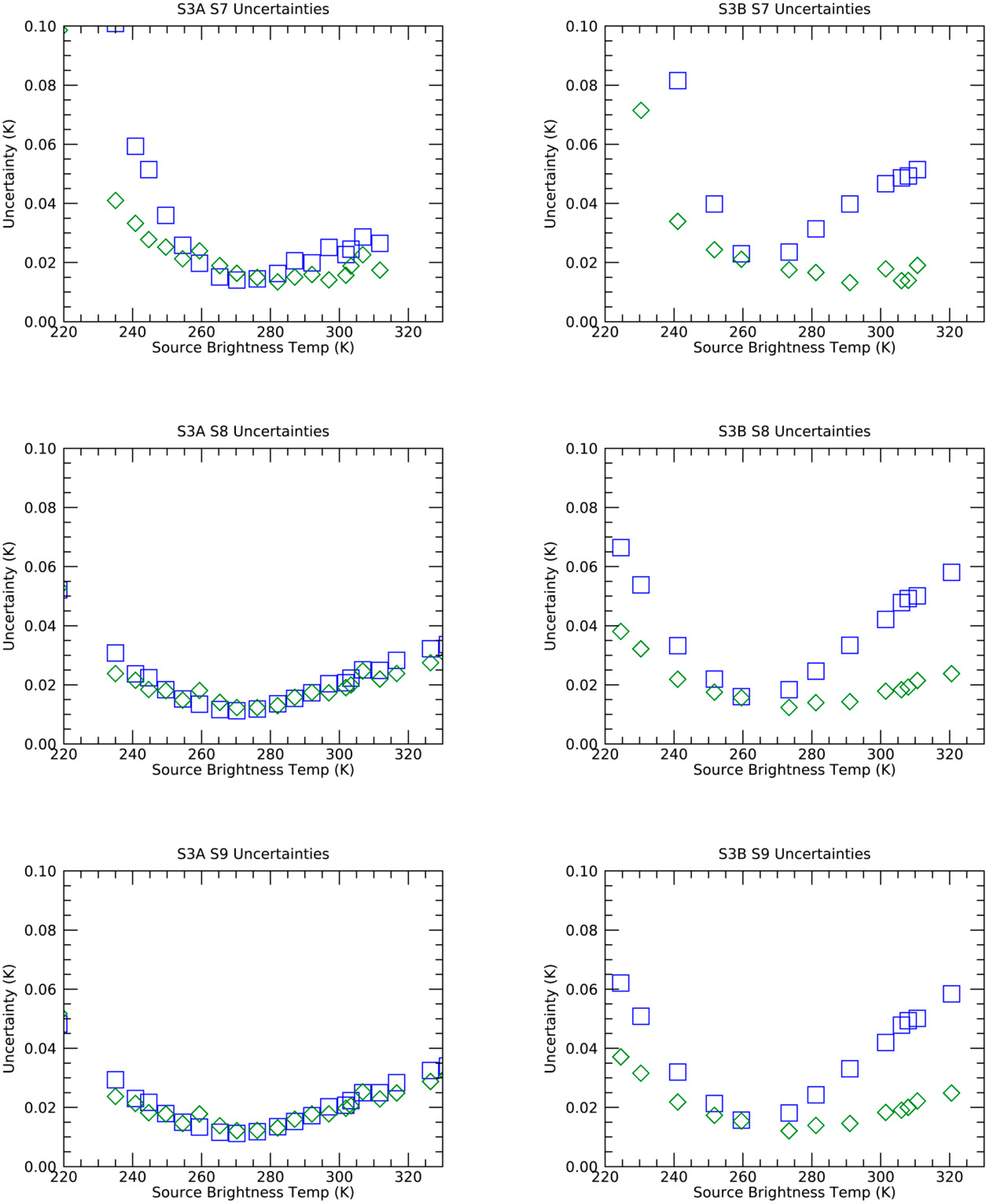
3.3. Radiometric Noise

The noise in counts, $\mathsf{\sigma }\mathrm{C}$ was recorded during each temperature plateaux of the external sources, Figure 6. For S7, we observe that the noise signal increases with source temperature, and is due to the increase in photon noise. The second feature is the noise at S7 drops sharply to a low value at scene temperatures >307 K due to the saturation of the detector. For S8 and S9, the main noise source is the intrinsic detector noise, so the instrument noise in counts should be constant with scene temperature. However, we observe a small variation in the noise signal with scene temperature for SLSTR-A due to residual photon noise.

At TIR wavelengths, the radiometric signal-to-noise performance is expressed as the Noise Equivalent Difference Temperature (NEDT):

$$\mathrm{N}\mathrm{E}\mathrm{D}\mathrm{T}=\mathrm{c}\mathrm{a}\mathrm{l}\_\mathrm{s}\mathrm{l}\mathrm{o}\mathrm{p}\mathrm{e} \mathsf{\sigma }\mathrm{C}{\frac{\mathrm{d}\mathrm{L}}{\mathrm{d}\mathrm{T}}|}_{\mathrm{T}}^{-1}$$

(14)

where

$$\mathrm{c}\mathrm{a}\mathrm{l}\_\mathrm{s}\mathrm{l}\mathrm{o}\mathrm{p}\mathrm{e}=\left({\mathrm{L}}_{\mathrm{B}\mathrm{B}1}-{\mathrm{L}}_{\mathrm{B}\mathrm{B}2}\right)/\overline{({\mathrm{C}}_{\mathrm{B}\mathrm{B}1}}-\overline{{\mathrm{C}}_{\mathrm{B}\mathrm{B}2}})$$

(15)

NEDTs for SLSTR-A and B are shown in Figure 7. The results show that the actual performance is much better than the goal requirement over the whole temperature range for S8 and S9 and for scene temperatures > 260 K for S7. For comparison, the predicted values from the design analysis which include margins for end-of-life performance are shown [14]. Note, the apparent non-linearity in NEDT with scene temperature which is primarily due to the form of dL/dT (derivative of the Planck function) that varies with temperature.

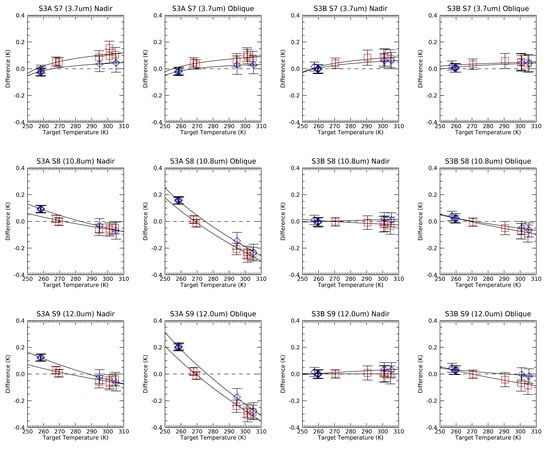
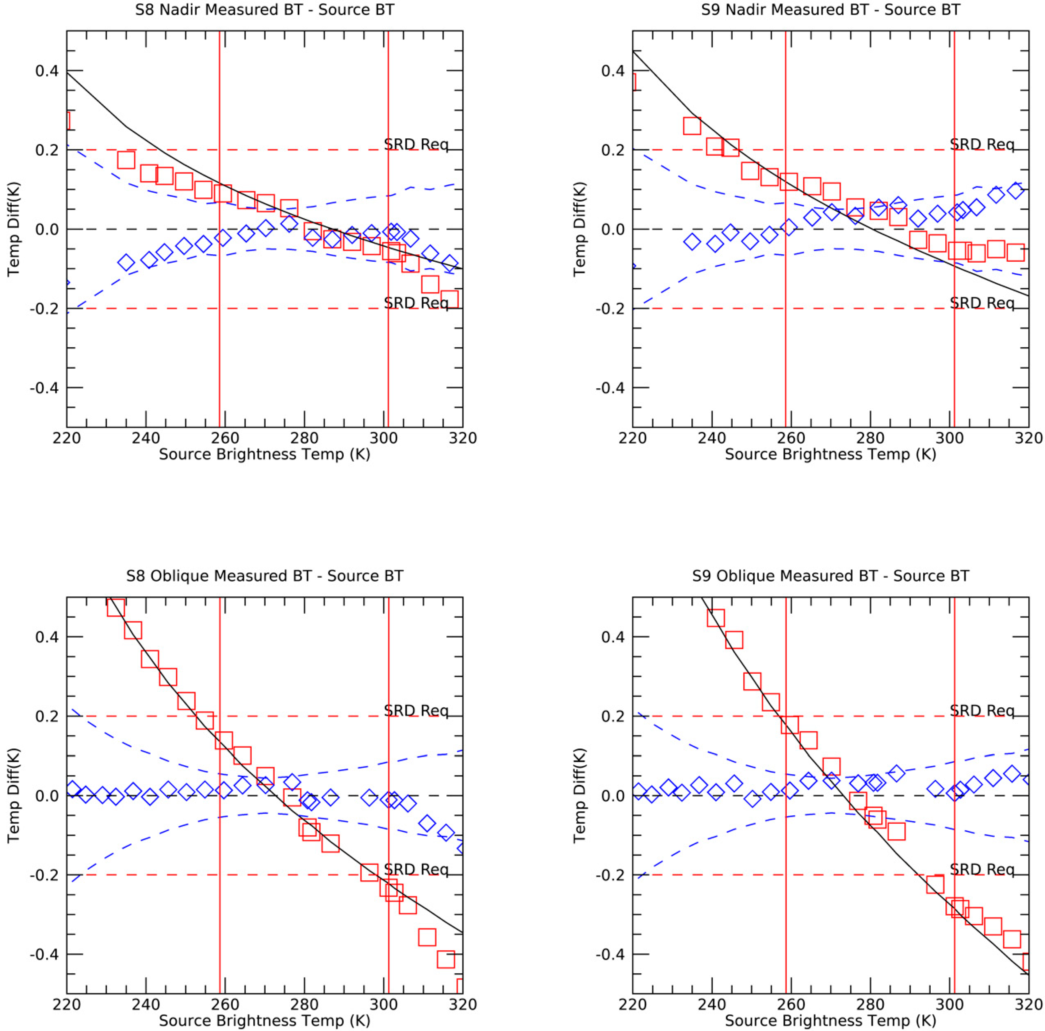
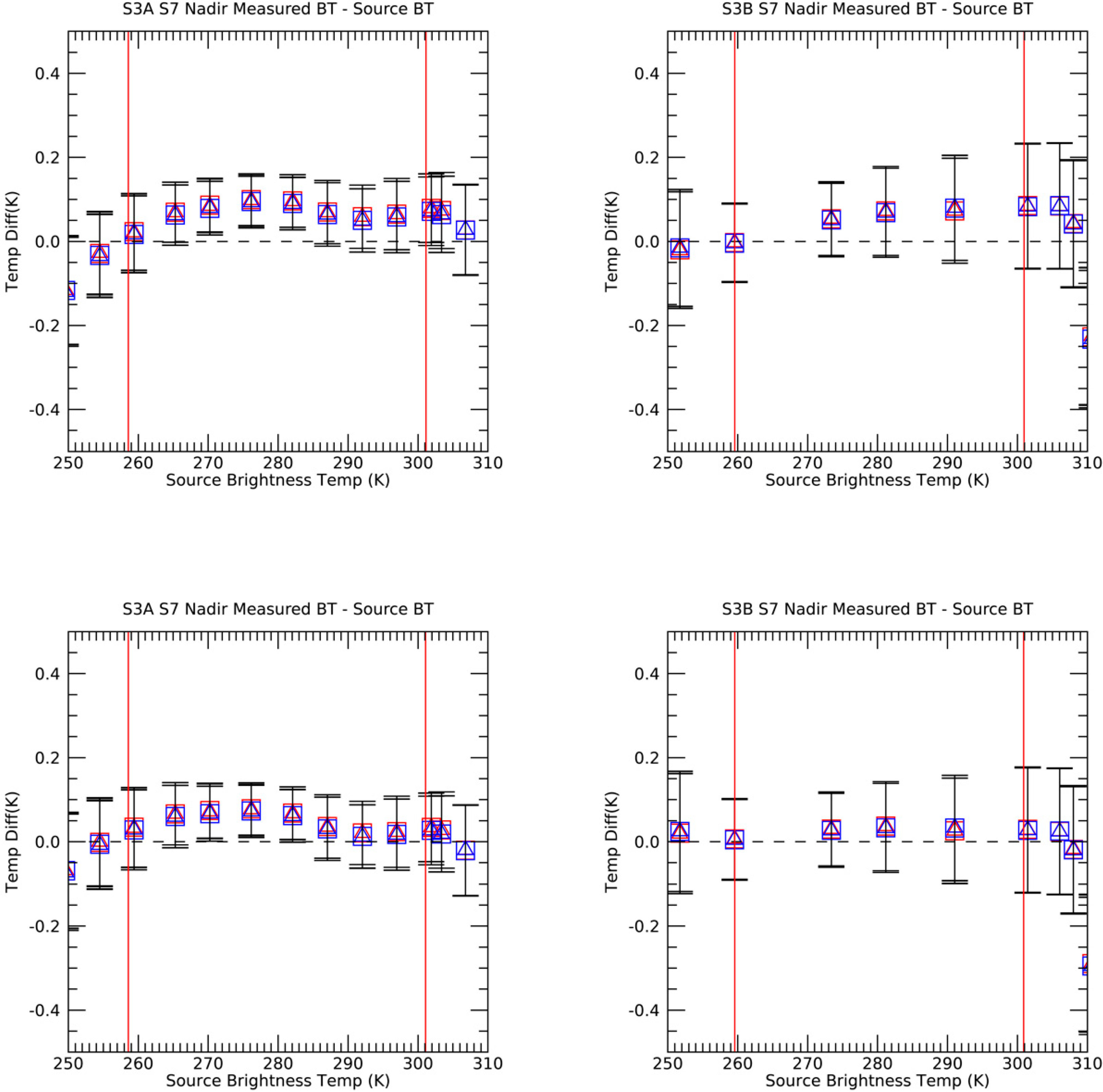
3.4. Comparisons with Scene Temperature

Using the radiometric calibration model, non-linearity curves and temperature-to-radiance look up tables, we convert the raw detector counts for each detector and integrator of each channel to derive the brightness temperatures. In Figure 8 and Figure 9, we compare the measured BTs against the actual external target BTs for SLSTR-A and B, respectively. The results for both SLSTR-A and B show that the measured BTs are within the threshold requirement of 0.2 K within the temperature range of the on-board BB temperatures that are critical for SST retrieval (as shown by the red lines). However, there is a significant discrepancy at the measurements outside the temperature range covered by the on-board BB temperatures, in particular for SLSTR-A (see Figure 8). In the nadir view we see differences at S8 and S9 of approximately +0.1 K for the −YBB (at 258 K) and −0.07 K for the +YBB (at 301 K), while for the oblique view the differences are higher, being 0.16 K for the −YBB and −0.26K for the +YBB. This was unexpected because the differences should be close to zero at the temperatures of the on-board BBs, particularly for the cold BB, which is at the same temperature as the OME, so should be close to an ideal BB. Possible causes and a proposed correction to these offsets are discussed in Section 4.1 of this paper.

For S7, in both SLSTR-A and SLSTR-B, the measured BTs agree within uncertainties for scene temperatures above 260 K. There is a small discrepancy of ~50 mK for scene temperatures of 300 K corresponding to the heated BB source. This will be discussed further in Section 4.2.

SLSTR-B is significantly better and is more in line with the expected behavior, especially for the nadir view, showing temperature differences <0.1 K within the range of the two on-board BBs (Figure 9).

3.5. Comparisons with Different On-Board BB Temperatures

The calibration was also verified with the on-board black bodies at different power levels, in addition to the nominal setting as reported in the previous section. These were with the +YBB heater off (floating) and the −YBB at 301 K, then 305 K, with the −YBB off (floating) and the +YBB at 305 K and then at 290 K before returning to the nominal configuration.

Where the external BB temperature is close to that of an on-board BB, errors due to calculation of radiometric gain and offset, non-linearity and spectral response become insignificant and only residual errors remain. For example, it is a direct comparison of the radiances of the internal and external BB sources, since from Equation (1) where X = 1, ${\mathrm{L}}_{\mathrm{scene}}={\mathrm{L}}_{\mathrm{BB}1}$ and where X = 0, ${\mathrm{L}}_{\mathrm{scene}}={\mathrm{L}}_{\mathrm{BB}2}$. So, for each of the calibration runs, measurements were taken with the external BB temperature matched to the on-board target temperatures to investigate these residuals. The differences between the brightness temperatures and actual target temperatures, for all tests at cold operational thermal environment, are shown in Figure 10. For all tests, we observe that the variation with scene temperature is consistent with the main calibration results reported in Figure 8 and Figure 9.

For S8 and S9, we note the following. First the differences for the unheated BB are much greater than expected since, when the BB cavity is close to that of the optics temperature, errors due to the non-blackness of the cavity should be negligible. Second, the differences for SLSTR-B are lower than for SLSTR-A and slightly different for the two internal BBs. This would point to an effect within the SLSTR instruments and not the external calibration sources, otherwise the magnitude should be the same. This will be discussed in Section 4.1.

For S7, the BT discrepancy where the BB is unheated is close to zero and increases with temperature. For SLSTR-A, the result is slightly different depending on which BB is heated. For SLSTR-B, the result is unaffected by the configuration and is of the same magnitude for nadir and oblique views. Because the differences at the cold BB temperatures are zero, a possible explanation would be an error in the flight BB emissivity as discussed in Section 4.2.

3.6. Response vs. Detector Temperature

Tests were performed with the IR Focal Plane Assemblies (FPAs) at an elevated temperature to provide needed information in the event of marginal performance of the SLSTR cryocoolers. It is known that the S8 and S9 detector response, noise and spectral response performances are sensitive to their temperature. The radiometric measurements were performed as for the nominal operational case, but with the IR FPA running at 92 K. This temperature was considered by the industrial team to be the upper limit that the FPA was likely to reach during the planned mission lifetime of 7.5 years. Higher temperatures were not considered because these were outside the range of predicted cooler temperatures.

The radiometric response corrected for non-linearity showed the same performance as for the nominal test cases, which confirm that the calibration error is not dependent on signal channel performance. The result also confirms that with the appropriate non-linearity correction, the same radiometric accuracy can be achieved with the higher detector temperature.

The radiometric noise values were slightly higher than for the nominal operating temperatures, but still within the 0.05 K requirements with some margin, (

Table 6. NEDTs in K and calibration slope in W·m⁻²·sr⁻¹·µm⁻¹ per count for scene temperature at ~270 K for nominal operating temperature and the elevated temperature. Detector temperatures are shown separately for each channel.

Model	Channel	Tdet (K)	NEΔT (K)	Calibration Slope (W·m−2·sr−1·µm−1)	Tdet (K)	NEΔT (K)	Calibration Slope (W·m−2·sr−1·µm−1)
SLSTR-A	S7	84.3	0.046	1.9039 × 10−5	89.2	0.046	1.9263 × 10−5
	S8	85.7	0.013	2.1987 × 10−4	90.6	0.015	2.5789 × 10−4
	S9	86.3	0.020	2.7104 × 10−4	91.2	0.026	3.5896 × 10−4
SLSTR-B	S7	85.3	0.033	1.5534 × 10−5	92.9	0.046	1.8036 × 10−5
	S8	85.3	0.014	2.6192 × 10−4	92.7	0.021	3.0744 × 10−4
	S9	85.6	0.017	2.5396 × 10−4	92.9	0.027	3.5049 × 10−4

). However, this was mainly due to a lower sensitivity of the detector response as indicated by the change in the calibration slope.

3.7. Comparisons vs. Earth View

It is essential that the radiometric calibration is consistent across the full field of view of SLSTR. Although the design concept should ensure this because the conical scanning geometry dictates that the angle of incidence of the incoming scene radiance at the scan mirror is constant, other factors such as stray light from the earth view baffles could cause scan dependent variations in the calibration biases.

The SLSTR calibration rig was specifically designed to allow the IR radiometric calibration around the full earth view by moving the two calibration sources. This approach follows that for the (A)ATSR instruments where the two external BBs were mounted on a rotating earth shine plate to move them around the scan cone. For SLSTR, because there are two separate scan cones it was necessary to move the two calibration sources independently along a track by means of a geared stepper motor.

Calibration measurements around the earth views were performed for scene temperatures of 240 K, 280 K and 300 K. The results in Figure 11 show that the absolute BT error is consistent with the center of view results within ±20 mK.

3.8. Orbital Simulation

So far all of the calibration measurements reported in this paper were performed with the instrument under stable, steady state thermal balance conditions. Although this is essential for minimizing uncertainties, the tests do not represent the actual flight conditions where orbital variations will affect the thermal stability of the instrument, in particular the earth view baffles. To demonstrate the radiometric performance under such transient conditions, orbital simulation tests were performed.

The instrument thermal modelling predicted that the strongest thermal variations would be caused by the changing solar illumination on the earth view baffles as well as the earth scene radiances when transitioning from day to night. Since the calibration facility does not include a solar simulator, the test was performed by varying only the earth-shine plate from −10 °C to +5 °C over 100 min. The thermal radiator targets and shroud temperatures were not changed during the test.

For SLSTR-A, the external BB sources were operated at set points of 310 K, 280 K and 240 K allowing 1 orbit for transition and 2 for performing the radiometric measurements. For SLSTR-B, the set-points were revised slightly to 300 K, 280 K and 250 K to allow a better evaluation of S7 channel which is affected by saturation above 307 K and has high NEDT at 240 K.

The results for SLSTR-A in Figure 12 shows the differences between the measured and actual source brightness temperatures. The results for S7 are in line with the steady state case results (e.g., RAD01, RAD02) and show little orbital variation. However, S8 and S9 both show strong orbital variations that are not seen in the actual BB temperatures. This reinforces the conclusion that the calibration errors observed in S8 and S9 are not due to errors in the BB thermometry, since they are spectrally dependent. For SLSTR-B (Figure 13) the absolute differences are much lower and there is no apparent variation with earth shine plate temperature.

Figure 14 shows the correlation of the SLSTR-A S9 calibration results for the orbital simulation with the earth shine plate temperatures and each of the internal instrument temperatures as measured by the TAEO thermometers. Here we see that there is a strong positive correlation with the instrument baffle temperatures, whereas there is a weak negative correlation with the earth-shine plate temperatures. This is strongly suggestive that the calibration error that we have detected is caused by something within the instrument itself and not external factors such as misalignment of the BB sources (which is unlikely considering that they are significantly oversized with respect to the instrument beam). The weakest correlations are with the instrument optics temperatures. This implies that the earth view baffles are contributing to the measured signals, which would imply a stray light error.

4. Discussion

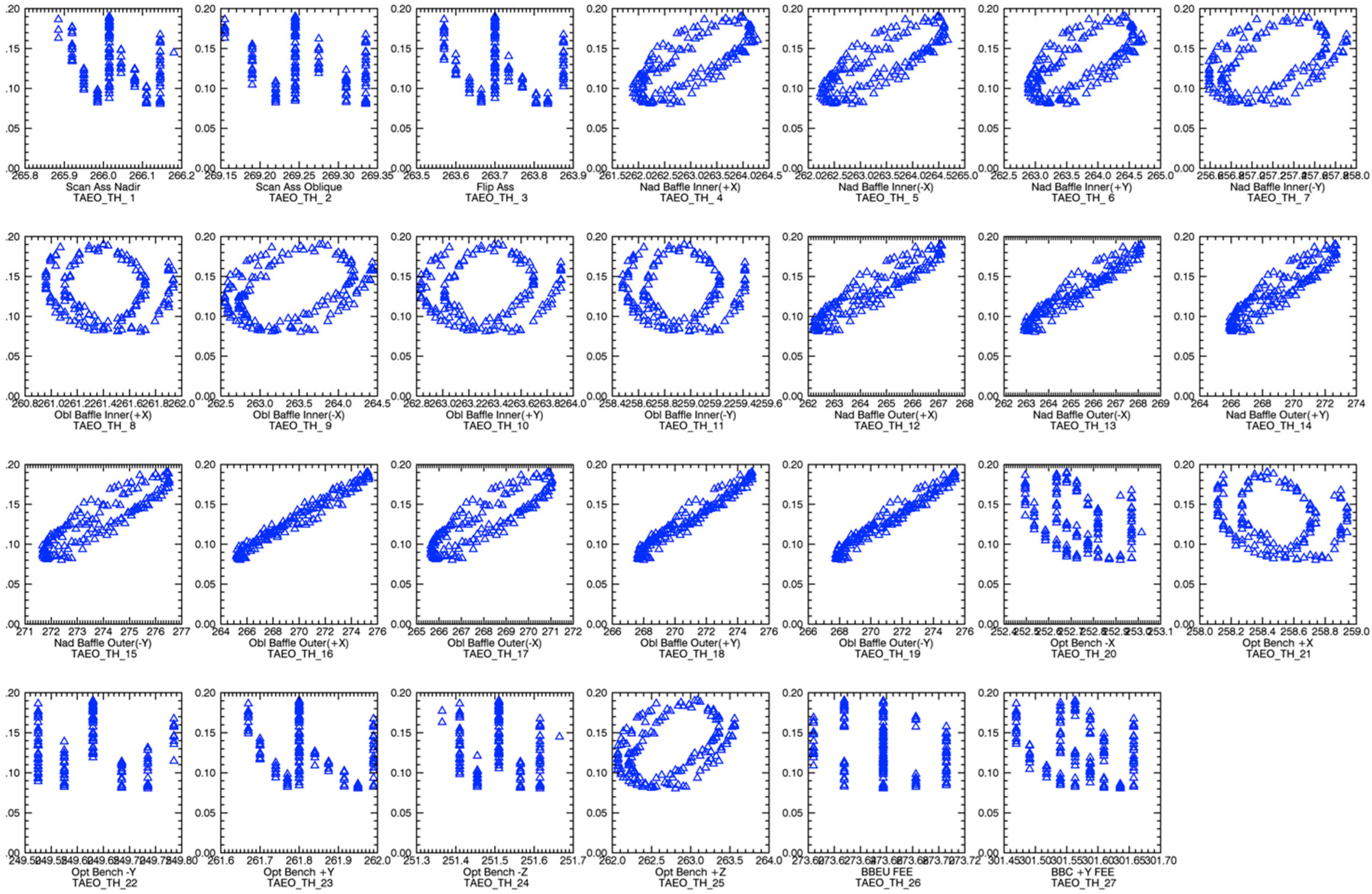
4.1. Stray Light’ Effect

The calibration results presented in this paper show that there were unexpected discrepancies in the brightness temperatures measured by SLSTR-A compared to the external reference. For model-B the results were significantly better for the nadir view, they still showed some differences in the oblique view, but within requirements. Because the result for SLSTR-A was non-compliant outside the temperature range of the on-board BBs an investigation was performed to establish the root cause and to identify a solution and allow a correction that takes into account the in-flight behavior [25].

As shown by the results presented here and analysis performed by the investigation it was deduced that the observed differences were dependent on:

• Configuration of the internal BBs
• Wavelength, with S9 (12 µm) being the worst affected.
• The thermal environment of the instrument.
• Appeared to be correlated with the external earth view baffle temperatures
• Stronger in oblique view than for nadir view

Because the effect is wavelength dependent, it was concluded that the calibration of the BB thermometers could not be the primary cause. It was also deduced that the differences were not affected by:

• Detector temperature
• Earth view position
• Optics temperatures
• External thermal environment
• Processing errors

The investigation by the project team concluded that the root cause was most likely due to lower than expected performance of the black coating used in the Parabolic Mirror Assembly (PMA) stop [25]. The PMA stop is designed to be the defining aperture of the SLSTR optical beam. Since the SLSTR detectors view an area slightly larger than the PMA, the stop contributes to detected IR signal. Hence, the stop must be sufficiently black to minimize any unwanted reflections from internal and external sources and be stable in temperature. Measurements of the black-coating material showed that the hemispherical reflectance at wavelengths > 10 µm were of the order 5–10%, making it the most likely candidate [26]. As a precaution, the SLSTR-B PMA was removed and recoated with a different coating with hemispherical reflectance 2–3% which appears to have reduced the radiometric offsets in S8 and S9, see Figure 9.

A basic approach is to assume that the stray light error is a linear function of the measured radiance and can be derived from the internal BB sources, so by arranging with Equation (1) we get:

$$\begin{array}{cc}{\mathsf{\Delta }\mathrm{L}}_{\mathrm{t}\mathrm{o}\mathrm{t}\mathrm{a}\mathrm{l}}\hfill & ={\mathrm{w}}_{\mathrm{s}\mathrm{t}\mathrm{r}\mathrm{a}\mathrm{y}}\left({\mathrm{L}}_{\mathrm{s}\mathrm{t}\mathrm{r}\mathrm{a}\mathrm{y}}-{\mathrm{L}}_{\mathrm{m}\mathrm{e}\mathrm{a}\mathrm{s}}\right)\hfill \\ \hfill & ={\mathrm{w}}_{\mathrm{s}\mathrm{t}\mathrm{r}\mathrm{a}\mathrm{y}}\left({\mathrm{L}}_{\mathrm{s}\mathrm{t}\mathrm{r}\mathrm{a}\mathrm{y}}-\left(\mathrm{X}{\mathrm{L}}_{\mathrm{B}\mathrm{B}1}+\left(1-\mathrm{X}\right){\mathrm{L}}_{\mathrm{B}\mathrm{B}2}\right)\right)\hfill \end{array}$$

(16)

We can obtain ${\mathrm{w}}_{\mathrm{s}\mathrm{t}\mathrm{r}\mathrm{a}\mathrm{y}}$ and ${\mathrm{L}}_{\mathrm{s}\mathrm{t}\mathrm{r}\mathrm{a}\mathrm{y}}$ and then ${\mathrm{T}}_{\mathrm{s}\mathrm{t}\mathrm{r}\mathrm{a}\mathrm{y}}$ by fitting to the measurements,

Table 7. Coefficients ${\mathrm{w}}_{\mathrm{s}\mathrm{t}\mathrm{r}\mathrm{a}\mathrm{y}}$ and ${\mathrm{L}}_{\mathrm{s}\mathrm{t}\mathrm{r}\mathrm{a}\mathrm{y}}$ and ${\mathrm{T}}_{\mathrm{s}\mathrm{t}\mathrm{r}\mathrm{a}\mathrm{y}}$ for the basic stray light model.

Instrument Model	View	Channel	wstray	Lstray (W·m−2·sr−1·µm−1)	Tstray (K)
SLSTR-A	Nadir	S8	0.003	6.883	280
		S9	0.004	7.001	280
	Oblique	S8	0.010	6.196	272
		S9	0.012	5.983	273
SLSTR-B	Nadir	S8	0.000	4.358	-
		S9	−0.000	3.681	246
	Oblique	S8	0.002	5.750	269
		S9	0.002	5.996	273

.

There are obvious limitations to the basic approach, mainly because the model does not address the sources of the stray light signals and does not account for the orbital simulation results. Furthermore, we would like to derive the stray light correction from measured temperatures within the instrument.

To understand how the stray light signal affects the calibration, we must return to the radiometric calibration model. A fundamental assumption is that both the gain and offset must remain constant during the calibration interval. If the offset is not constant during the scan cycle (which is the time between two calibration measurements), then we have a scan dependent perturbation of ±ΔL(pos) which in turn gives rise to a perturbation in the background signal ±ΔC(pos). Updating the calibration model in Equation (1) gives:

$${\mathrm{L}}_{\mathrm{scene}}+{\mathsf{\Delta }\mathrm{L}}_{\mathrm{scene}}=\mathrm{X}\left({\mathrm{L}}_{\mathrm{BB}1}+{\mathsf{\Delta }\mathrm{L}}_{\mathrm{BB}1}\right)+\left(1-\mathrm{X}\right)\left({\mathrm{L}}_{\mathrm{BB}2}+{\mathsf{\Delta }\mathrm{L}}_{\mathrm{BB}2}\right)$$

(17)

In the calibration processing performed in this report, we have assumed the ideal calibration model (Equation (1)), so the total error we observe in the measured radiance is

$${\mathsf{\Delta }\mathrm{L}}_{\mathrm{total}}={\mathsf{\Delta }\mathrm{L}}_{\mathrm{scene}}-{\mathrm{X}\mathsf{\Delta }\mathrm{L}}_{\mathrm{BB}1}-\left(1-\mathrm{X}\right){\mathsf{\Delta }\mathrm{L}}_{\mathrm{BB}2}$$

(18)

We equate this to a brightness temperature error, ${\mathsf{\Delta }\mathrm{T}}_{\mathrm{total}}$ using Equation (7).

We then have to determine ${\mathsf{\Delta }\mathrm{L}}_{\mathrm{scene}}$, ${\mathsf{\Delta }\mathrm{L}}_{\mathrm{BB}1}$ and ${\mathsf{\Delta }\mathrm{L}}_{\mathrm{BB}2}$. Let us assume that the scene radiance within the field of view of the instrument is a combination of the radiance emitted by the source (earth, BB) and a stray light signal. The scene radiance is then given by

$${\mathrm{L}}_{\mathrm{m}\mathrm{e}\mathrm{a}\mathrm{s}}=\left(1-{\mathrm{w}}_{\mathrm{s}\mathrm{t}\mathrm{r}\mathrm{a}\mathrm{y}}\right){\mathrm{L}}_{\mathrm{s}\mathrm{c}\mathrm{e}\mathrm{n}\mathrm{e}}+{\mathrm{w}}_{\mathrm{s}\mathrm{t}\mathrm{r}\mathrm{a}\mathrm{y}}{\mathrm{L}}_{\mathrm{s}\mathrm{t}\mathrm{r}\mathrm{a}\mathrm{y}}$$

(19)

where ${\mathrm{w}}_{\mathrm{s}\mathrm{t}\mathrm{r}\mathrm{a}\mathrm{y}}$ is the stray light factor and ${\mathrm{L}}_{\mathrm{s}\mathrm{t}\mathrm{r}\mathrm{a}\mathrm{y}}$ is the radiance from an external source.

If we substitute back into the error model, we obtain each term

$$\begin{array}{l}\Delta {\mathrm{L}}_{\mathrm{s}\mathrm{c}\mathrm{e}\mathrm{n}\mathrm{e}}={\mathrm{w}}_{\mathrm{s}\mathrm{t}\mathrm{r}\mathrm{a}\mathrm{y},\mathrm{s}\mathrm{c}\mathrm{e}\mathrm{n}\mathrm{e}}\left({\mathrm{L}}_{\mathrm{s}\mathrm{t}\mathrm{r}\mathrm{a}\mathrm{y},\mathrm{s}\mathrm{c}\mathrm{e}\mathrm{n}\mathrm{e}}-{\mathrm{L}}_{\mathrm{s}\mathrm{c}\mathrm{e}\mathrm{n}\mathrm{e}}\right)\\ \Delta {\mathrm{L}}_{\mathrm{B}\mathrm{B}1}={\mathrm{w}}_{\mathrm{s}\mathrm{t}\mathrm{r}\mathrm{a}\mathrm{y},\mathrm{B}\mathrm{B}1}\left({\mathrm{L}}_{\mathrm{s}\mathrm{t}\mathrm{r}\mathrm{a}\mathrm{y},\mathrm{B}\mathrm{B}1}-{\mathrm{L}}_{\mathrm{B}\mathrm{B}1}\right)\\ \Delta {\mathrm{L}}_{\mathrm{s}\mathrm{c}\mathrm{e}\mathrm{n}\mathrm{e}}={\mathrm{w}}_{\mathrm{s}\mathrm{t}\mathrm{r}\mathrm{a}\mathrm{y},\mathrm{s}\mathrm{c}\mathrm{e}\mathrm{n}\mathrm{e}}\left({\mathrm{L}}_{\mathrm{s}\mathrm{t}\mathrm{r}\mathrm{a}\mathrm{y},\mathrm{s}\mathrm{c}\mathrm{e}\mathrm{n}\mathrm{e}}-{\mathrm{L}}_{\mathrm{s}\mathrm{c}\mathrm{e}\mathrm{n}\mathrm{e}}\right)\end{array}$$

(20)

This presents a challenge because there are six degrees of freedom in the model (three stray light factors and three stray radiances) with a high degree of correlation, a limited number of test cases from the measurements. However, we make the following assumptions:

• We know from the orbital simulations (Figure 12 and Figure 14) that there is a strong correlation between the calibration results and the instrument baffle temperatures. This would allow us to determine ${\mathrm{w}}_{\mathrm{s}\mathrm{t}\mathrm{r}\mathrm{a}\mathrm{y},\mathrm{s}\mathrm{c}\mathrm{e}\mathrm{n}\mathrm{e}}$ and ${\mathrm{L}}_{\mathrm{s}\mathrm{t}\mathrm{r}\mathrm{a}\mathrm{y},\mathrm{s}\mathrm{c}\mathrm{e}\mathrm{n}\mathrm{e}}$ independently from contributions of the internal BB sources.
• We can then deduce ${\mathrm{w}}_{\mathrm{s}\mathrm{t}\mathrm{r}\mathrm{a}\mathrm{y},\mathrm{B}\mathrm{B}1}$, ${\mathrm{L}}_{\mathrm{s}\mathrm{t}\mathrm{r}\mathrm{a}\mathrm{y},\mathrm{B}\mathrm{B}1}$ and ${\mathrm{w}}_{\mathrm{s}\mathrm{t}\mathrm{r}\mathrm{a}\mathrm{y},\mathrm{B}\mathrm{B}2}$, ${\mathrm{L}}_{\mathrm{s}\mathrm{t}\mathrm{r}\mathrm{a}\mathrm{y},\mathrm{B}\mathrm{B}2}$ from the measurements where X = 0 and X = 1.
• The physical source of the stray light signal must be within the vicinity of the main signal and determined by the measured temperatures. So, for the earth views these will be the external baffles, and for the internal BB sources these will be the optical enclosure.

Using these assumptions, we were able to determine the stray light coefficients in

Table 8. Stray light coefficients ${\mathrm{w}}_{\mathrm{s}\mathrm{t}\mathrm{r}\mathrm{a}\mathrm{y}}$ for the stray light model derived from the measurements and the hemispherical reflectance of the black coatings, ρ_black, used for the primary aperture stop.

Instrument Model	View	Channel	wstray,scene	wstray,bb1/bb2	ρblack
SLSTR-A	Nadir	S8	0.0110	0.0095	5%
		S9	0.0120	0.0090
	Oblique	S8	0.0120	0.0350	10%
		S9	0.0158	0.0500
SLSTR-B	Nadir	S8	0.0044	0.0014	2%
		S9	0.0060	0.0025
	Oblique	S8	0.0048	0.0038	5%
		S9	0.0079	0.0045

from all the test results.

Using the modelled stray light error and uncertainties, we have applied these to the radiometric calibration results and reduces the differences for all scene temperatures, Figure 15. The model was verified for all test conditions (cold and hot thermal conditions, different BB temperatures, orbital simulations and view position). It must be emphasized that this is an approximation to the radiometric error and assumes that the correction is the same on-ground and on-orbit.

Post-launch comparisons of SLSTR-A with IASI [27] showed that the nadir view data were in good agreement with the reference sensor for scene temperatures below 290 K. The result suggested that the stray light error was not present as anticipated and the proposed corrections would have overcorrected the data and degraded the data quality further without adaptation. Hence it was not employed in the Level-1 data processing chain. This does not mean that the stray light model itself was incorrect, but most likely the stray-light effect was less significant for the nadir view on-orbit. Results from tandem phase comparisons of SLSTR-A and B performed under the Sentinel-3 Tandem for Climate (S3T4C) project [28] showed good agreement between SLSTR-A and B in the nadir view, but showed the presence of the stray light effect in the oblique view, primarily for SLSTR-A, consistent with the results of this paper. Further investigations are in progress to determine improvements to the stray light model that account for the in-orbit behavior.

4.2. S7 Emissivity

As reported in Section 3.5, we have observed a discrepancy in the S7 channel results that varies with scene temperature. The difference is smallest when the BB source is at the same temperature as the thermal environment, which would imply an error in the reported cavity emissivity. Using the measurements, and adapting the model of Equation (20) we can determine corrections for the emissivity of the cavities at this wavelength to minimize the differences (

Table 9. Original and corrected on-board BB emissivities for channel S7. Uncertainty estimates for the error are derived from the fit to the measurements.

	SLSTR-A			SLSTR-B
	εreported	Δε	εcorrected	εreported	Δε	εcorrected
+YBB	0.99830 ± 0.00012	−0.0020 ± 0.0020	0.9963 ± 0.0020	0.99830 ± 0.00012	−0.0025 ± 0.0020	0.9958 ± 0.0020
−YBB	0.99830 ± 0.00012	−0.0045 ± 0.0020	0.9938 ± 0.0020	0.99830 ± 0.00012	−0.0030 ± 0.0020	0.9953 ± 0.0020

and Figure 16).

A possible explanation of the differences in S7 may relate to the spectral reflectance of the black-coating. The cavity emissivity was derived from reflectance measurements of the black-coating material and a Monte Carlo ray-tracing model to account for the cavity geometry [11]. Spectral reflectance measurements of witness samples of the black-coating material performed by NIST show a peak in the emissivity from 3–6 µm with significant variance between measurements, Figure 17. Between 8 and 14 µm, the reflectance is spectrally flat and below 1% for all samples. This would suggest that the cavity emissivity is more sensitive to variations in the coating reflectance at S7 than for S8 and S9. Likewise, it would imply that the reported uncertainty in the cavity emissivity is underestimated as it does not account for all effects.

4.3. Saturation of S7

The calibration tests showed that the S7 channel saturates at a scene temperature around 305 K for the nominal integration time of 70 µs which was much lower than the requirement of 323 K. The instrument design allows the saturation level to be increased by reducing the integration time of the channel. Assuming that the response is linear with integration time, it should be possible to predict the maximum temperature as L_max(t_int) = L_max(70 µs) × 70/t_int. To investigate this further, it was decided to perform all the radiometric calibration tests at different integration times of 70 (default), 50 and 38 µs. An Automatic Test Procedure (ATP) was used to cycle through these integration times at two-minute intervals for each BB temperature plateau.

In Figure 18 we observed that the increase in expected T_max is in line with predictions. For a 50 µs integration time, the radiometric noise was still within specification and the calibration results were in line with the 70 µs results. Below 50 µs non-linearity is affected and noise was not in specification with the goal requirements, (see

Table 10. SLSTR-A NEDT vs. integration time.

NEΔT at 270 K	Tint = 70 µs	Tint = 50 µs	Tint = 38 µs	EOL Req. Goal/Threshold
S7	40 mK	50 mK	60 mK	50 mK/80 mK
S8	18 mK	19 mK	20 mK	30 mK/50 mK
S9	20 mK	25 mK	30 mK	30 mK/50 mK

).

Because SLSTR is a scanning instrument however, the integration time affects the pixel field of view on the ground. The SST and LST retrieval algorithms are dependent on the co-registration and matching pixel area on ground of the TIR channels. Therefore, because of the potential impact on the scientific data quality the shorter integration times for S7 were not implemented, accepting the saturation as this has a low impact on SST retrievals.

5. Conclusions

In this paper, we have presented the main results of the radiometric calibration tests for the SLSTR-A and B TIR channels. The calibration results demonstrated that the radiometric noise performance exceeded the requirements and was within the predicted budget. The measurements were used to derive non-linearity corrections for all channels and could be used for all instrument configurations. Results for SLSTR-A showed that comparisons at the internal BB temperatures show higher than expected BT differences, particularly at the cold internal BB temperature where errors due to emissivity should be negligible (since the BB should be close to the background thermal environment). An analysis of the results suggested that the most likely cause of the error was due to a stray light source that is not accounted for by the calibration algorithm. This led to a modification in the black-coating used for SLSTR-B, which resulted in an improvement in the BT differences. After correcting for non-linearity and stray light effects, the BTs measured by both SLSTRs agreed within the 0.1 K goal over the range 240 K to 320 K. Analysis of the Sentinel-3 tandem phase comparisons of SLSTR-A and B level-1 radiometric data reported in [28] has since reported differences in the oblique view data which are consistent with the calibration results reported in this paper, and application of the simplified stray light model to the tandem phase results has reduced the differences.

Measurements performed under different thermal environments and for different internal BB temperatures show consistent results. Measurements around the earth views show that the calibration accuracy is constant around the scan.

The calibration tests have validated the on-board calibration systems, and the processing algorithms and auxiliary data used in the operational data processing system to convert from raw data to calibrated radiances and brightness temperature. Results from the instrument-level calibration tests provide key inputs into the level-1 data processing chain, in-particular the non-linearity tables and stray light correction factors.

The SLSTR level-1 data products provide uncertainty estimates that are derived from the ground calibration. Radiometric noise estimates (random effects) are derived from the on-board BB sources and provided per scan. Estimates of the uncertainties in the radiometric calibration (correlated effects) are provided as a table of uncertainty vs. scene temperature/radiance in the quality datasets associated with each channel and view.

Preparations are currently in progress for the pre-launch calibration of the SLSTR-C and D instruments to be performed at RAL Space. The test campaigns for these instruments will build on the experience of the ATSR and SLSTR-A/B sensors to maintain the traceability of the calibration across the complete mission series.

Validation of the ground BB sources by measurement of an independent reference radiometer, such as the NPL Amber radiometer [19] will ensure the continued traceability of the pre-launch calibration, and provide an additional link the calibration to the shipborne radiometers used for providing in-situ Fiducial Reference Measurement (FRM).

References

1. Ohring, G.; Wielicki, B.; Spencer, R.; Emery, B.; Datla, R. Satellite instrument calibration for measuring global climate change. Bull. Am. Meteorol. Soc. 2005, 86, 1303–1313. [Google Scholar] [CrossRef]
2. Liua, X.; Wub, W.; Wielickia, B.A.; Yangb, Q.; Kizerb, S.H.; Huangc, X.; Chenc, X.; Katoa, S.; Sheaa, Y.L.; Mlynczaka, M.G. Spectrally Dependent CLARREO Infrared Spectrometer Calibration Requirement for Climate Change Detection. J. Clim. 2017, 30, 3979–3998. [Google Scholar] [CrossRef]
3. Drinkwater, M.R.; Rebhan, H. Sentinel-3 Mission Requirements Document and References Therein. In Sentinel-3 Project Document, EOP-SMO/1151/MD-md; ESA, ESTEC: Noordwijk, The Netherlands, 2007; Available online: http://esamultimedia.esa.int/docs/GMES/GMES_Sentinel3_MRD_V2.0_update.pdf (accessed on 3 August 2020).
4. Donlon, C.; Berruti, B.; Buongiorno, A.; Ferreira, M.-H.; Féménias, P.; Frerick, J.; Goryl, P.; Klein, U.; Laur, H.; Mavrocordatos, C.; et al. The Global Monitoring for Environment and Security (GMES) Sentinel-3 Mission. Remote. Sens. Environ. 2012, 120, 37–57. [Google Scholar] [CrossRef]
5. Llewellyn-Jones, D.; Remedios, J. The Advanced Along Track Scanning Radiometer (AATSR) and its predecessors ATSR-1 and ATSR-2: An introduction to the special issue. Remote. Sens. Environ. 2012, 116, 1–3. [Google Scholar] [CrossRef]
6. Závody, A.M.; Mutlow, C.T.; Llewellyn-Jones, D.T. A radiative-transfer model for sea-surface temperature retrieval for the Along-Track Scanning Radiometer. J. Geophys. Res. Ocean. 1995, 100, 937–952. [Google Scholar] [CrossRef]
7. Coppo, P.; Ricciarelli, B.; Brandani, F.; Delderfield, J.; Ferlet, M.; Mutlow, C.; Munro, G.; Nightingale, T.; Smith, D.; Bianchi, S.; et al. SLSTR: A high accuracy dual scan temperature radiometer for sea and land surface monitoring from space. J. Mod. Opt. 2010, 57, 1815–1830. [Google Scholar] [CrossRef]
8. Coppo, P.; Mastrandrea, C.; Stagi, M.; Calamai, L.; Nieke, J. Sea and Land Surface Temperature Radiometer detection assembly design and performance. J. Appl. Remote. Sens. 2014, 8, 084979. [Google Scholar] [CrossRef]
9. Hawkins, G.; Sherwood, R.; Djotni, K.; Coppo, P.; Höhnemann, H.; Belli, F. Cooled Infrared Filters and Dichroics for the Sea and Land Surface Temperature Radiometer (SLSTR). Appl. Opt. 2013, 52, 2125–2135. [Google Scholar] [CrossRef] [PubMed]
10. Mason, I.M.; Sheather, P.H.; Bowles, J.A.; Davies, G. Blackbody calibration sources of high accuracy for a spaceborne infrared instrument: The along Track Scanning Radiometer. Appl. Opt. 1996, 35, 629–639. [Google Scholar] [CrossRef] [PubMed]
11. Nightingale, T.J.; McPheat, R.; Smith, D.L.; Mortimer, H.; Polehampton, E.; Lee, A. Sentinel-3A/B SLSTR spectral response calibration (Manuscript in preparation).Spectral Responses and Test Reports are Available for Download at. Available online: https://sentinel.esa.int/web/sentinel/technical-guides/sentinel-3-slstr/instrument/measured-spectral-response-function-data (accessed on 23 June 2020).
12. SLSTR BlackBody Subsystem & Temperature Acquisition Electronics Technical Budgets Report. In Sentinel-3 Project Document, S3-RP-ABS-SL-0017; ESA, ESTEC: Noordwijk, The Netherlands, 2012.
13. Peters, D.; Etxaluze, M.; Smith, D. Report on BBS Emissivity and Sensitivity to Temperature Gradients. In Sentinel-3 Project Document, S3-RP-RAL-SL-114; RAL Space: Harwell, UK, 2018. [Google Scholar]
14. Smith, D.L.; Nightingale, T.J.; Mortimer, H.; Middleton, K.; Edeson, R.; Cox, C.V.; Mutlow, C.T.; Maddison, B.J.; Coppo, P. Calibration approach and plan for the sea and land surface temperature radiometer. J. Appl. Remote. Sens. 2014, 8, 84980. [Google Scholar] [CrossRef]
15. Smith, D.; Mutlow, C.; Delderfield, J.; Watkins, B.; Mason, G. ATSR infrared radiometric calibration and in-orbit performance. Remote. Sens. Environ. 2012, 116, 4–16. [Google Scholar] [CrossRef]
16. Mason, G. Test and Calibration of the Along Track Scanning Radiometer, A Satellite-Borne Infrared Radiometer Designed to Measure Sea Surface Temperature. Ph.D. Thesis, University of Oxford, Oxford, UK, 1991. [Google Scholar]
17. Monte, C. ATSR BB Emissivity Measurements. Private Communication. 2012. Available online: https://ioccg.org/wp-content/uploads/2015/02/optical-radiometry-excerpt.pdf (accessed on 23 June 2020).
18. Prokhorov, A.; Prokhorova, N.I. Application of the three-component bidirectional reflectance distribution function model to Monte Carlo calculation of spectral effective emissivities of nonisothermal blackbody cavities. Appl. Opt. 2012, 51, 8003–8012. [Google Scholar] [CrossRef] [PubMed]
19. Theocharous, E.; Fox, N.P. CEOS comparison of the IR Brightness temperature measurements in support of satellite validation. Part II: Laboratory comparisons of the brightness temperature of blackbodies. NPL Rep. OP3 2010. Available online: http://eprintspublications.npl.co.uk/id/eprint/4744 (accessed on 3 August 2020).
20. JASMIN. Available online: http://Jasmin.ac.uk (accessed on 4 June 2020).
21. Joint Committee for Guides in Metrology, Evaluation of Measurement Data. Guide to the Expression of Uncertainty in Measurement (JCGM 100:2008). Available online: https://www.bipm.org/utils/common/documents/jcgm/JCGM_100_2008_E.pdf (accessed on 30 July 2019).
22. Smith, D.; Hunt, S.; Wooliams, E.; Etxaluze, M.; Peters, D.; Nightingale, T.; Mittaz, J. Traceability of the Sentinel-3 SLSTR Level-1 Infrared Radiometric Processing. (Unpublished; Manuscript in preparation).
23. Theocharous, E.; Ishii, J.; Fox, N.P. Absolute linearity measurements on HgCdTe detectors in the infrared region. Appl. Opt. 2004, 43, 4182–4188. [Google Scholar] [CrossRef] [PubMed]
24. Yang, S.; Vayyshenker, I.; Li, X.; Scott, T. Accurate Measurement of Optical Detector Nonlinearity Proc. In Proceedings of the Natl. Conf. Stds. Labs., Chicago, IL, USA, 3 July–4 August 1994. [Google Scholar]
25. Mavrocordatos, C. SLSTR LWIR channels calibration issue: Pre-launch Status. In Sentinel-3 Project Document S3-TN-ESA-SL-0663; ESA, ESTEC: Noordwijk, The Netherlands, 2016. [Google Scholar]
26. Adibekyan, A.; Kononogova, E.; Monte, C.; Hollandt, J. High-Accuracy Emissivity Data on the Coatings Nextel 811–21, Herberts 1534, Aeroglaze Z306 and Acktar Fractal Black. Int. J. Thermophys. 2017, 38, 89. [Google Scholar] [CrossRef] [Green Version]
27. Tomazic, I.; O’Carroll, A.; Hewison, T.; Ackerman, J.; Donlon, C.; Nieke, J.; Andela, B.; Coppens, D.; Smith, D. Initial comparison between Sentinel-3A SLSTR and IASI aboard MetOp-A and MetOp-B. GSICS Q. 2016, 10. [Google Scholar] [CrossRef]
28. Hunt, S.E.; Mittaz, J.P.D.; Smith, D.L.; Polehampton, E.; Yemelyanova, R.; Woolliams, E.R.; Donlon, C. A Level 1 and Level 2 Comparison of the Sentinel-3A/B SLSTR Tandem Phase Data using Metrological Principles. Remote Sens. 2020. (Under review). [Google Scholar]
Figure 1. The Sea and Land Surface Temperature Radiometers (SLSTR)-B Instrument in the Space Test Chamber (STC) clean room at RAL Space under preparation for the infrared radiometric calibration tests.
Remotesensing 12 02510 g001
Figure 2. SLSTR calibration rig under preparation for thermal testing showing the main components. (a) earth shine plate, (b) nadir view BB source, (c) oblique view BB source, (d) spacecraft simulator, (e) cold thermal panels, (f) instrument electronics enclosure, (g) field of view optics and (h) space test chamber.
Remotesensing 12 02510 g002
Figure 3. Uncertainty estimates at k = 1 for SLSTR-A and SLSTR-B calibration tests. Green diamonds, = uncertainties in the reference brightness temperatures derived from the external BB thermometers and emissivity. Blue squares, = uncertainties in the SLSTR measurements derived from the instrument calibration model.
Remotesensing 12 02510 g003
Figure 4. SLSTR-A (left) and SLSTR-B (right) nadir view measured detector counts vs. scene radiances and brightness temperatures for channels S7–S9. The oblique view shows a similar behavior and is not displayed for that reason. The corresponding scene temperature is shown in the lower axes. = Detector 1, Integrator 1; = Detector 1, Integrator 2; Δ = Detector 2, Integrator 1; Δ = Detector 2, Integrator 2. The SLSTR Thermal Infrared (TIR) channels have two detector elements in the along-track direction and are read out in alternate integration cycles, which are calibrated separately.
Remotesensing 12 02510 g004
Figure 5. SLSTR-A (left) and SLSTR-B (right) non-linearity responses expressed as percentage for channels S7-S9. = Detector 1, Integrator 1; = Detector 1, Integrator 2; Δ = Detector 2, Integrator 1; Δ = Detector 2, Integrator 2.
Remotesensing 12 02510 g005
Figure 6. Detector noise in counts vs. brightness temperature for SLSTR-A (left) and SLSTR-B (right) nadir view for channels S7–S9. The values for the oblique view are not shown as they are very close to the values for the nadir view. = Detector 1, Integrator 1; = Detector 1, Integrator 2; Δ = Detector 2, Integrator 1; Δ = Detector 2, Integrator 2.
Remotesensing 12 02510 g006
Figure 7. SLSTR-A (left) and SLSTR-B (right) nadir view measured Noise Equivalent Difference Temperature (NEDT) vs. brightness temperatures for channels S7–S9. The values for the oblique view are not shown as they are very close to the values for the nadir view. = Detector 1, Integrator 1; = Detector 1, Integrator 2; Δ = Detector 2, Integrator 1; Δ = Detector 2, Integrator 2. The red curve corresponds to the predicted values, and the dashed red line shows the System Requirements Definition (SRD) target requirements.
Remotesensing 12 02510 g007
Figure 8. Differences between brightness temperatures of the external BB sources measured by SLSTR-A and the actual BB brightness temperatures. The vertical red-lines correspond to the temperatures of the on-board s. = Detector 1, Integrator 1; = Detector 1, Integrator 2; Δ = Detector 2, Integrator 1; Δ = Detector 2, Integrator 2. Error bars represent the combined uncertainty of the measurement at k = 3.
Remotesensing 12 02510 g008
Figure 9. Differences between brightness temperatures of the external BB sources measured by SLSTR-B and the actual BB brightness temperatures. The vertical red-lines correspond to the temperatures of the on-board s. = Detector 1, Integrator 1; = Detector 1, Integrator 2; Δ = Detector 2, Integrator 1; Δ = Detector 2, Integrator 2. Error bars represent the combined uncertainty of the measurement at k = 3.
Remotesensing 12 02510 g009
Figure 10. Results for all measurements where the external BB sources were at the same temperatures as the instrument s. The plot shows the differences between brightness temperatures of the external sources measured by SLSTR-A (left) and SLSTR-B (right) and the actual BB brightness temperatures. The red squares correspond to the normally heated +Y BB, the blue diamonds correspond to the normally cold −Y BB. Error bars correspond to uncertainties at k = 3.
Remotesensing 12 02510 g010
Figure 11. Results for calibration at different positions around the earth view for a scene temperature of 300 K. Plots show the relative difference in BT as compared to the values at center of the earth views which is indicated by the red line. Note that fewer measurements for SLSTR-A were possible due to operational issues of the BB motors. These were resolved and the full scan for SLSTR-B could be performed. = Detector 1, Integrator 1; = Detector 1, Integrator 2; Δ = Detector 2, Integrator 1; Δ = Detector 2, Integrator 2.
Remotesensing 12 02510 g011
Figure 12. SLSTR-A Orbital simulation results showing the differences between the measured and actual source brightness temperatures. = Detector 1, Integrator 1; = Detector 1, Integrator 2; Δ = Detector 2, Integrator 1; Δ = Detector 2, Integrator 1. Error bars are not shown for clarity.
Remotesensing 12 02510 g012
Figure 13. SLSTR-B Orbital simulation results showing the differences between the measured and actual source brightness temperatures. = Detector 1, Integrator 1; = Detector 1, Integrator 2; Δ = Detector 2, Integrator 1; Δ = Detector 2, Integrator 2. Error bars are not shown for clarity.
Remotesensing 12 02510 g013
Figure 14. Correlations of SLSTR-A nadir view calibration temperature differences (vertical axes) against internal instrument temperatures from TAEO thermometers (horizontal axes) measured during the orbital simulation tests.
Remotesensing 12 02510 g014
Figure 15. SLSTR-A S8 and S9 BT differences after adjusting for the stray light error. Uncorrected; Corrected data; Stray-Light Model; -- Combined uncertainty (k = 3).
Remotesensing 12 02510 g015
Figure 16. S7 BT differences before (top) and after adjusting (bottom) the instrument BB emissivity to the corrected values in Table 9. = Detector 1, Integrator 1; = Detector 1, Integrator 2; Δ = Detector 2, Integrator 1; Δ = Detector 2, Integrator 2. Error bars represent the combined uncertainty at k = 3.
Remotesensing 12 02510 g016
Figure 17. Spectral reflectance of the black-coating used for the SLSTR A and B BB cavities measured by NIST, and the resulting effective cavity emissivity from 2 to 20 µm [13]. At channel S7 (3.7 mm) the reflectivity of shows strong variation as a function of wavelength, but also from sample to sample suggesting a larger uncertainty of the cavity’s emissivity in this spectral channel.
Remotesensing 12 02510 g017
Figure 18. Comparison of measured (blue squares) against predicted (solid line) maximum brightness temperature Tmax vs. integration time for S7 channel.
Remotesensing 12 02510 g018