Assessing the Effect of Tandem Phase Sentinel-3 OLCI Sensor Uncertainty on the Estimation of Potential Ocean Chlorophyll-a Trends

Abstract

The Sentinel-3 tandem project represents the first time that two ocean colour satellites have been flown in the same orbit with minimal temporal separation (~30 s), thus allowing them to have virtually identical views of the ocean. This offers an opportunity for understanding how differences in individual sensor uncertainty can affect conclusions drawn from the data. Here, we specifically focus on trend estimation. Observational chlorophyll-a uncertainty is assessed from the Sentinel-3A Ocean and Land Colour Imager (OLCI-A) and Sentinel-3B OLCI (OLCI-B) sensors using a bootstrapping approach. Realistic trends are then imposed on a synthetic chlorophyll-a time series to understand how sensor uncertainty could affect potential long-term trends in Sentinel-3 OLCI data. We find that OLCI-A and OLCI-B both show very similar trends, with the OLCI-B trend estimates tending to have a slightly wider distribution, although not statistically different from the OLCI-A distribution. The spatial pattern of trend estimates is also assessed, showing that the probability distributions of trend estimates in OLCI-A and OLCI-B are most similar in open ocean regions, and least similar in coastal regions and at high northern latitudes. This analysis shows that the two sensors should provide consistent trends between the two satellites, provided future ageing is well quantified and mitigated. The Sentinel-3 programme offers a strong baseline for estimating long-term chlorophyll-a trends by offering a series of satellites (starting with Sentinel-3A and Sentinel-3B) that use the same sensor design, reducing potential issues with cross-calibration between sensors. This analysis contributes an important understanding of the reliability of the two current Sentinel-3 OLCI sensors for future studies of climate change driven chlorophyll-a trends.

1. Introduction

Sentinel-3 is a multi-satellite Copernicus mission featuring a number of instruments, including an optical radiometry instrument, focused on measuring the Earth’s surface over land and oceans with the aim of supporting environmental and climate monitoring [1]. The optical instrument aboard Sentinel-3 is known as the Ocean and Land Colour Imager (OLCI). Sentinel-3A was launched on the 16 February 2016, followed by Sentinel-3B on the 25 April 2018. A further two satellites (Sentinel-3C and Sentinel-3D) are planned for launch to maintain a minimum operational period of over 20 years for the Sentinel-3 mission. During the period from June to October 2018, Sentinel-3A and Sentinel-3B were flown in a tandem configuration with a separation of just 30 s in their overpass time. This tandem phase was designed to ensure the consistency of data between the two satellites in support of establishing reliable long-term climate data records in accordance with the Global Climate Observing System’s Climate Monitoring Principles [2]. A specific project, known as “Sentinel-3 Tandem for Climate”, was set up to analyse the data in this period [3]. This paper focuses on assessing the ability of the OLCI data to provide a reliable climate data record which can be used to study long-term chlorophyll-a (chl-a) change.

Ocean colour satellite records allow us to assess how global phytoplankton biomass may be changing, including due to the effects of climate change. The high spatial coverage and frequent revisit time makes ocean colour satellite records particularly well suited to this task [4]. However, the short lifespan of any individual sensor, relative to the timescales over which climate change trends in chl-a become detectable against the large magnitude of chl-a variability on seasonal to interannual timescales [5,6,7], presents a major challenge to reliable trend detection using the ocean colour record. A meta-analysis of observational studies has shown this effect, with shorter datasets proving more likely to have conflicting, and larger magnitude, trend estimates compared to longer records [8]. Studies have also suggested that it may require a chl-a record of ~30 years in order to reliably separate a climate change driven chl-a trend from natural variability [6,9].

In order to compensate for the short lifespan of individual ocean colour records, datasets from multiple sensors can be merged such as has been done (by merging data from the individual Sea-Viewing Wide Field-of-View Sensor (SeaWiFS), MEdium Resolution Imaging Spectrometer (MERIS), Moderate Resolution Imaging Spectroradiometer (MODIS), and Visible Infrared Imaging Radiometer Suite (VIIRS) instruments) for the GlobColour and ESA OC-CCI products [10,11,12]. In order for multiple sensors to be successfully used together it is necessary to compensate for any differences between the individual datasets, which may arise due to differences in the following: radiometric bands, spatial resolution, calibration, atmosphere and aerosol corrections, and corrections for sun glint and white caps [13]. The Sentinel-3 programme offers a planned continuous record of over 20 years with sensors of a quasi-identical design (small changes to the Sentinel-3 C and D sensors are planned), which will negate a number of these effects. However, subtle differences (a result of material tolerances, manufacture, and pre-flight characterisation) between the two identically designed OLCI sensors, may lead to measurement differences. The Sentinel-3 Tandem phase offers a unique opportunity to quantify the effect of any differences on our ability to estimate chl-a trends in future Sentinel-3 OLCI records. In this study, the differences in chl-a uncertainty from the Sentinel-3 A and B sensors during the tandem phase will be used to understand the effect of uncertainty due to differences in radiometric calibration on the ability to estimate potential long-term trends in a series of synthetic chl-a time series.

2. Materials and Methods

Chl-a data for this study come from two different OLCI datasets. The first one is collected by the Payload Data Ground Segment with OLCI-A being vicariously adjusted at L2 but not OLCI-B. The second one is provided by a custom reprocessing of OLCI-A and OLCI-B where OLCI-A has been radiometrically aligned to OLCI-B based on the analysis of tandem phase L1 data [14]. No system vicarious calibration (SVC) has been applied to OLCI-A in this reprocessing as the radiometric alignment to OLCI-B is changing the instrument calibration, making the operational SVC meaningless. The OLCI-B radiometry has not been modified in both datasets and, as no SVC is performed on OLCI-B yet, the comparison between the two OLCI-A processings (one with SVC, one with alignment to OLCI-B) thus provides a useful validation of the radiometric alignment against the current operational setup [15]. It is worth mentioning that OLCI-B vicarious calibration shall be performed in the near future, see [15], for further discussions on the subject.

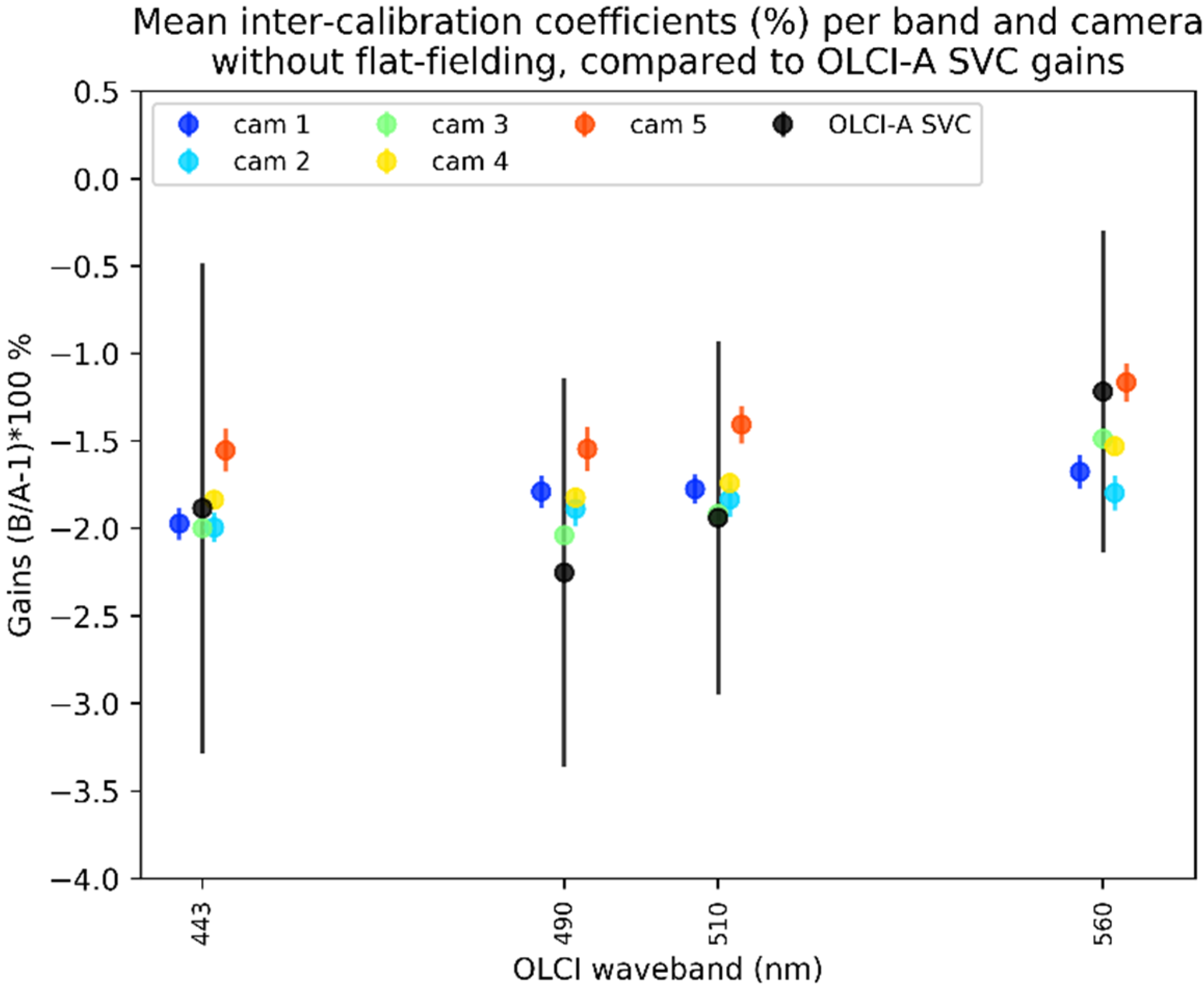
In each L2 processing, OLCI chl-a is calculated from normalised water-leaving reflectance using the OC4Me algorithm [16]. This algorithm relies on the maximum band ratio obtained from reflectance at 443, 490, or 510 nm against reflectance at 560 nm. As OLCI-A SVC and alignment to OLCI-B provide a radiometric adjustment at L1 it is worth mentioning the order of magnitude of the adjustments performed on OLCI-A radiances. Figure 1 (adapted from [15]) shows a comparison between the corresponding coefficients for all four bands involved in the computation of OC4Me chl-a. SVC gains are provided with the uncertainty associated to the dispersion of individual matchups used for computing the average values; these are quite large but in line with uncertainties common in cross-calibration comparisons. Inter-calibration to OLCI-B is shown as the mean per camera with very small standard deviations according to the extremely high precision allowed by the tandem cross-calibration [14]. It can be seen that both SVC and harmonisation provide roughly the same order of magnitude for adjusting OLCI-A with discrepancies up to about 0.5%.

The SVC gains of OLCI-A in the visible bands are retrieved after a preliminary relative adjustment of the near-infrared bands [15], the fact that such adjustment is not performed for OLCI-B and OLCI-A aligned shall provide most differences with OLCI-A vicariously adjusted where strong aerosols optical thickness encountered. Indeed, atmospheric correction handles the retrieval of atmospheric aerosol properties (optical thickness and aerosol types) from the two near-infrared bands at 779 and 865 nm [17]. Atmospheric corrections are performed as detailed by the documents in the Sentinel 3 document library (https://sentinel.esa.int/web/sentinel/user-guides/sentinel-3-olci/document-library).

It is also worth mentioning the fact that OLCI-A/OLCI-B harmonisation is based on the observation of clouds providing the strongest and whitest signal closest to what is obtained from on-board solar diffusers. Slight differences against a harmonisation based on comparisons over water targets are underlined by small centred differences, not exceeding 5%, seen in L2 Water products [15]. The reflectance ratio in the OC4Me algorithm allows chl-a products to be reasonably well aligned, with only a small amount of noise.

From a Plate Carrée reprojection of L2 chl-a products, daily L3 composites are computed notably through the filtering of sun glint and potentially cloud-contaminated pixels. A full description of the methods used for aligning and/or creating these datasets can be found in [14]. Only data during the tandem phase, where both OLCI-A and OLCI-B are available, are used, i.e., a total of 8 days, once a week, covering a period between 7 June 2018 and 16 October 2018. As the datasets are limited to a relatively small temporal period, an additional dataset is used to form a baseline for a longer synthetic time-series: the ESA OC-CCI v3.1 product (available at: http://www.esa-oceancolour-cci.org/ [11]). This dataset combines data from multiple sensors (SeaWiFS, MERIS, MODIS, and VIIRS) using both band-shifting and bias correction techniques to create an L3 dataset covering the period from September 1997 to June 2018 inclusive, producing an ~20 year time series comprised of daily data. These data are regridded to 1° spatial resolution to allow a more robust analysis (see below), at the cost of less variety in the background data. After regridding, the time series is then detrended in each grid cell (a Generalised Least-Square (GLS) regression process is used to estimate the natural chl-a trend, which is then subtracted from the time series). Detrending provides a time series with no trend, so a known trend can be imposed, whilst still including seasonal and interannual variability as well as missing data. This series forms a synthetic time series baseline by including features expected in the long-term Sentinel-3 data.

All OLCI-A and OLCI-B values within 1° grid cells over the 8 days available of tandem data were assessed to produce a variance estimate for each grid cell. Aggregating to 1° allows more samples to be incorporated within a grid cell, increasing reliability. Using the variance assessed from the OLCI data (for A-Aligned, A-Vicarious, and B separately), random zero-mean noise was added to the baseline series described above. Using random sampling from the zero-mean noise distribution, a series of 100 bootstraps per 1° grid cell were produced, creating a series of synthetic time series (for A-Aligned, A-Vicarious, and B separately) representing a range of observational noise. Once the “observational” noise had been added to the detrended time series, a series of synthetic trends in a realistic range determined from prior studies (±2%·yr⁻¹ [5,7,18,19,20]), were imposed on the time series. The range of trend values allow us to assess the interaction between the noise and trend magnitude/direction.

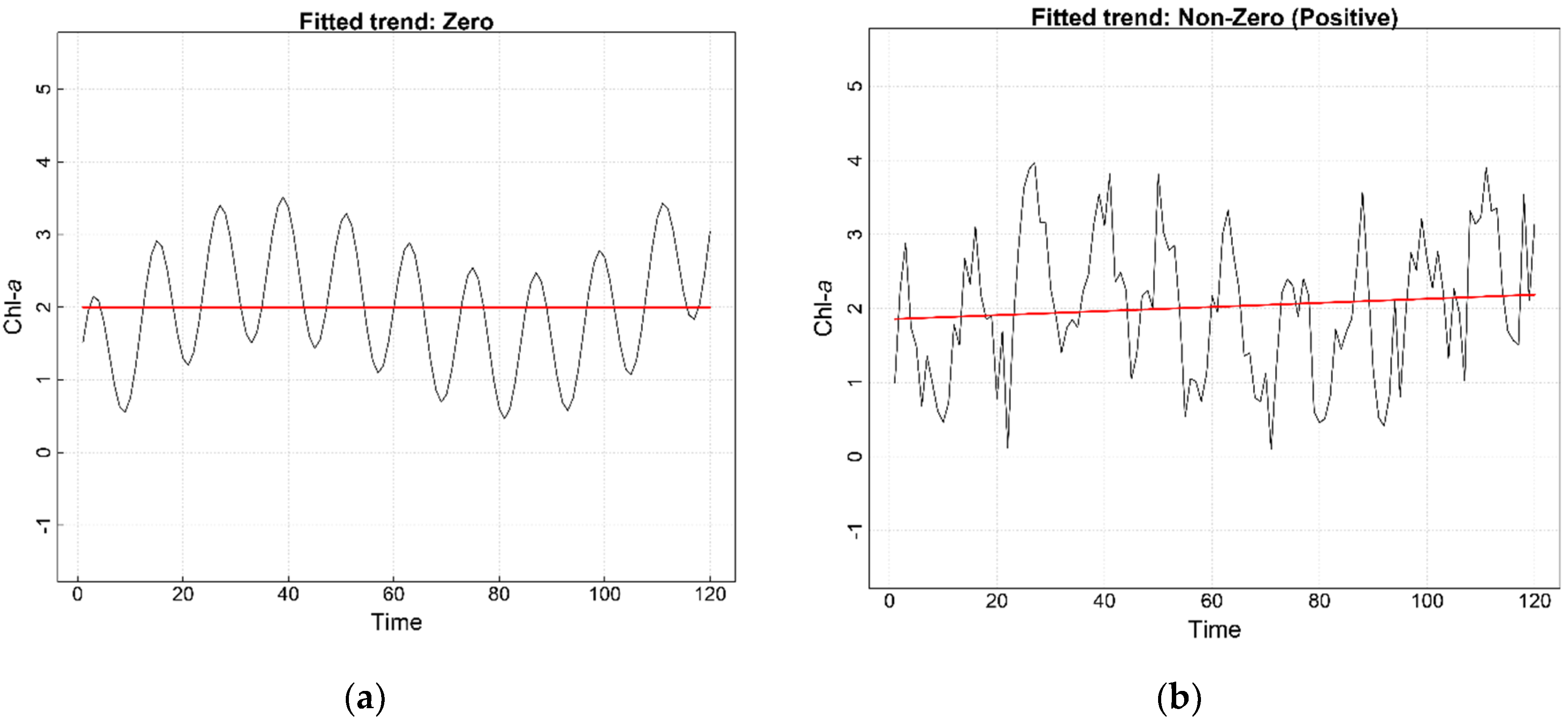
Finally each of the bootstraps of these synthetic time-series were analysed using GLS regression techniques, with temporal autocorrelation assuming an AR(1) process, to produce a chl-a trend estimate for each bootstrap. Without the addition of noise, the trend estimate would be exactly the same as the input chl-a trend. By adding the “observational” uncertainty, some variation around this is expected. A diagram showing the theory of this effect is included as Figure 2. The differences in the variations in trend estimates between the two sensors can then be assessed to understand the quantitative effect of this “observational” noise, with the comparison allowing us to effectively remove other noise contributions, as during the tandem phase OLCI-A and OLCI-B viewed the same scenes. Levene’s test [21] was used to determine if the difference in the variances of chl-a trend estimates in the pairs of datasets analysed was statistically significant.

3. Results

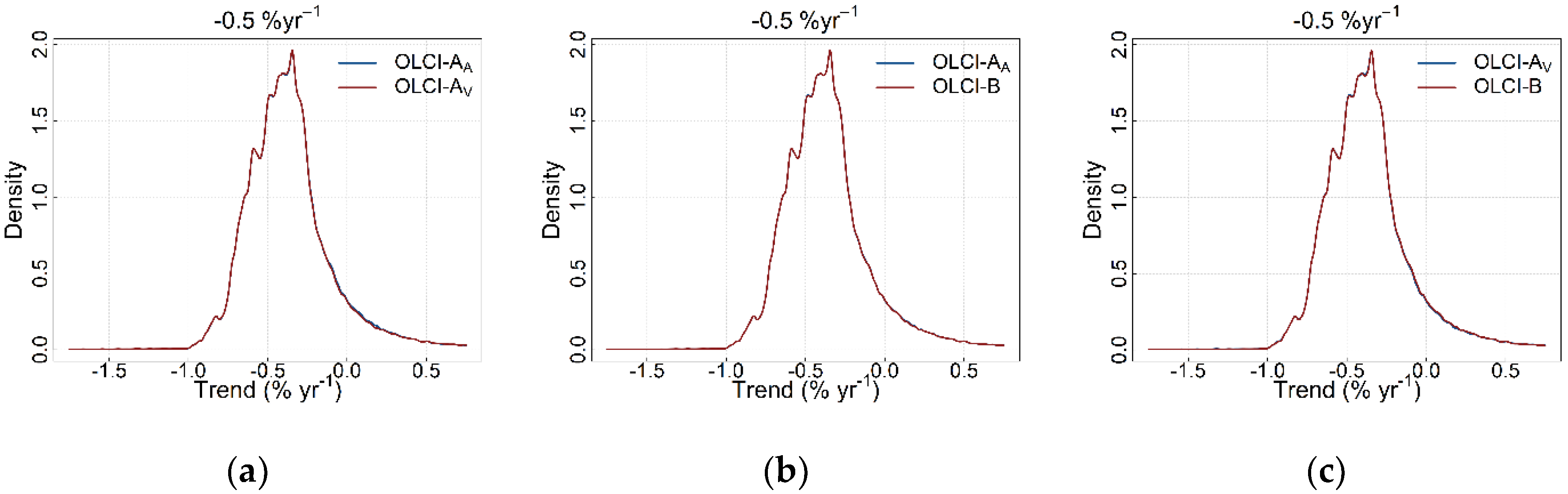
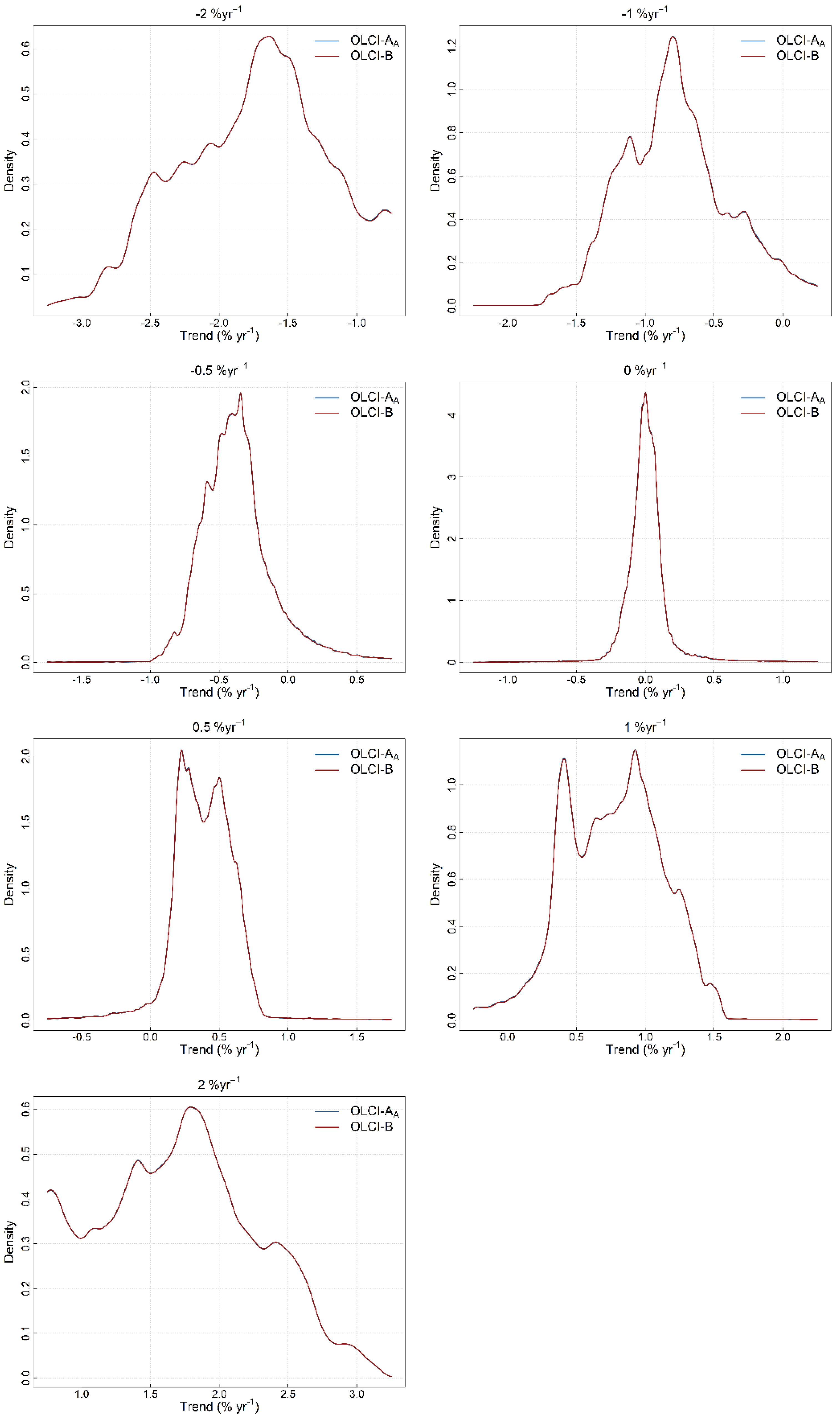
The probability density function of all chl-a trend estimates from all bootstraps across all global grid cells for an input trend of −0.5%·yr⁻¹ is shown in Figure 3. From this it can be seen that the peak of the distribution, i.e., the modal value, is ~−0.5%·yr⁻¹, the same as the input trend for all the comparisons. Some variability can be seen around this peak; all distributions have a standard deviation of ~0.27%·yr⁻¹. All distributions show some asymmetry, which can be attributed to the trends being estimated using log transformed chl-a data before being converted for plotting. 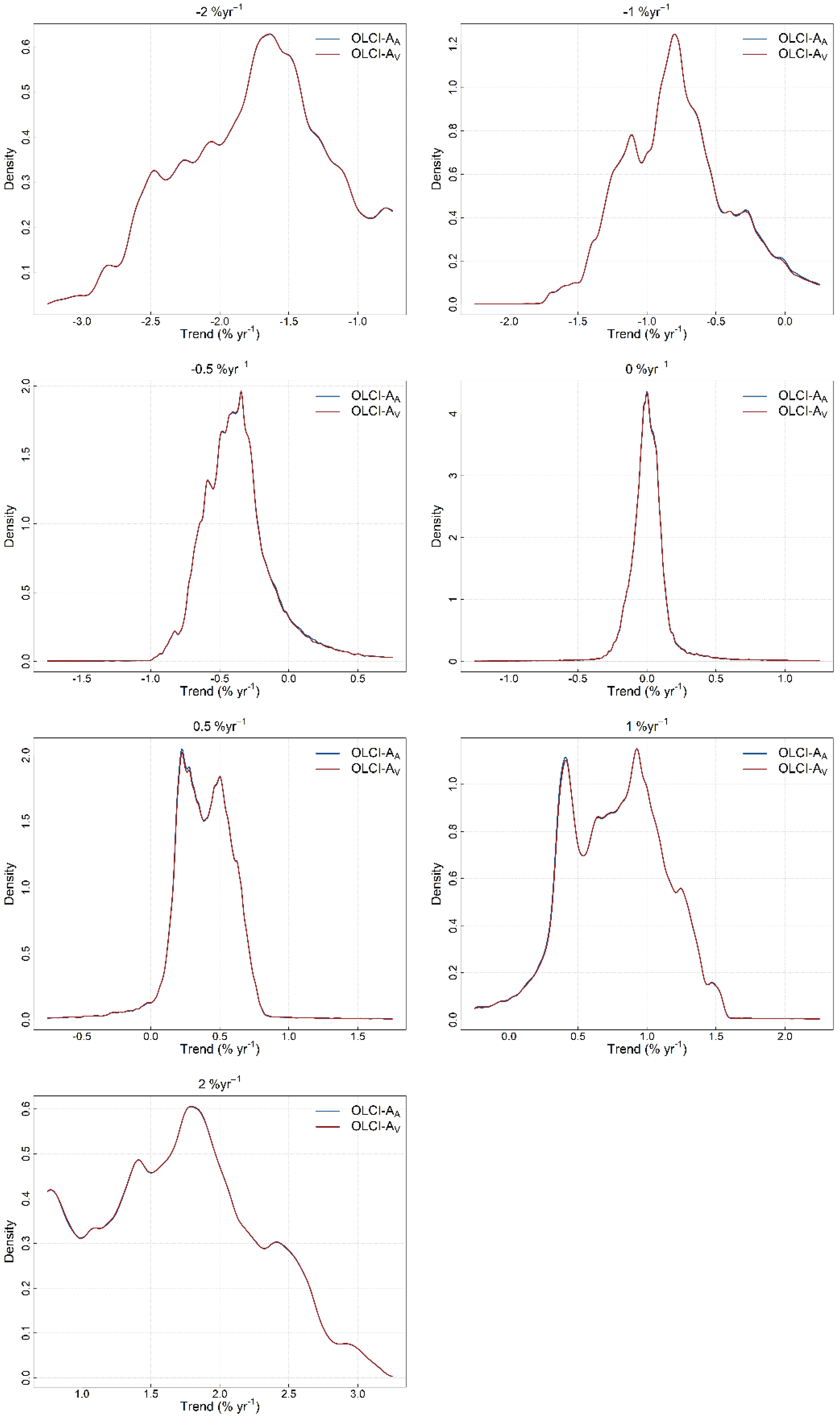It can be seen that for the three datasets OLCI-A-Aligned and OLCI-B are the most similar (expected from how OLCI-A-Aligned is created [14]) and that OLCI-A-Vicarious has a slightly, but negligibly, larger standard deviation of trend estimates (0.266%·yr⁻¹ for OLCI-A-Aligned, 0.272%·yr⁻¹ for OLCI-A-Vicarious, and 0.268%·yr⁻¹ for OLCI-B). These differences would not be expected to lead to any appreciable difference in trend detection when comparing the datasets. A realistic range of chl-a trends was tested, with very similar results in terms of consistency between datasets, although the standard deviation of trend estimates does increase with increasing values of input trend, and non-normal distributions indicate interactions with the underlying dataset (see Appendix A).

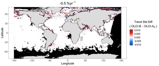
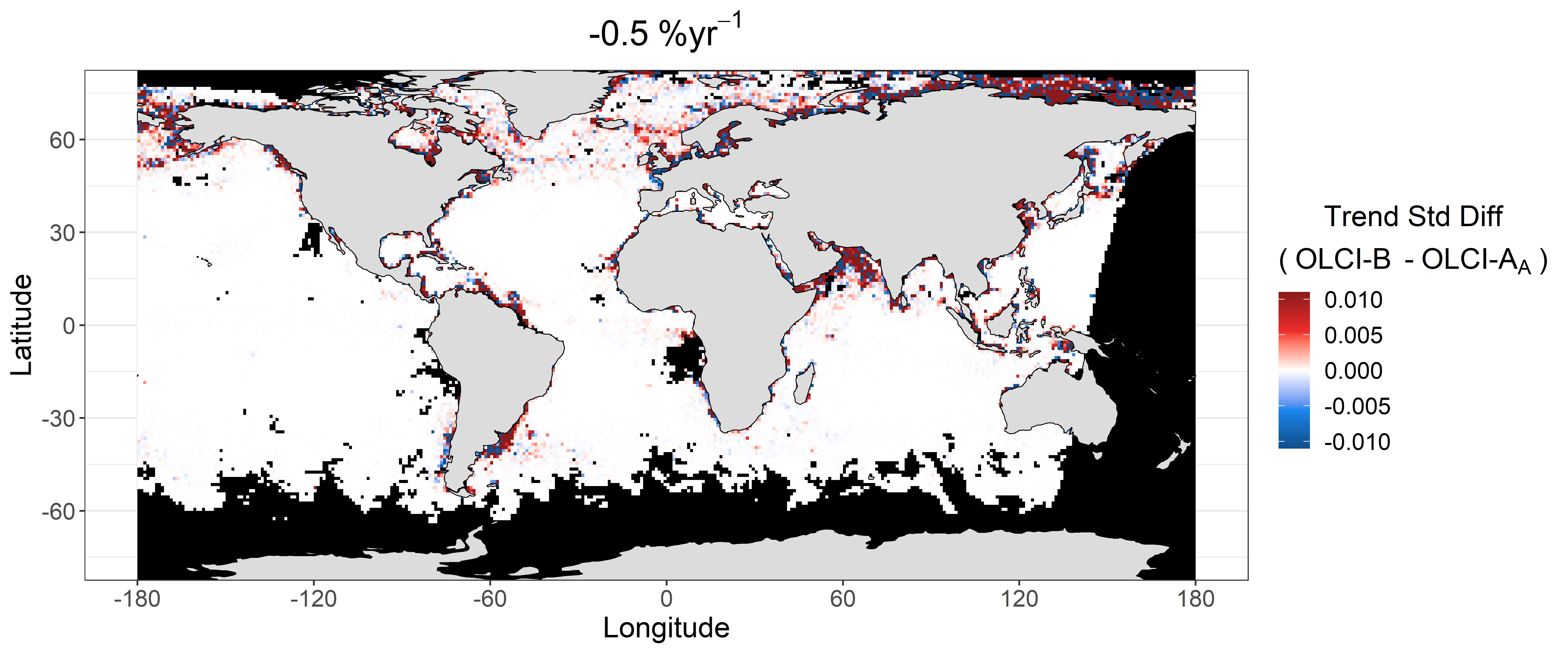
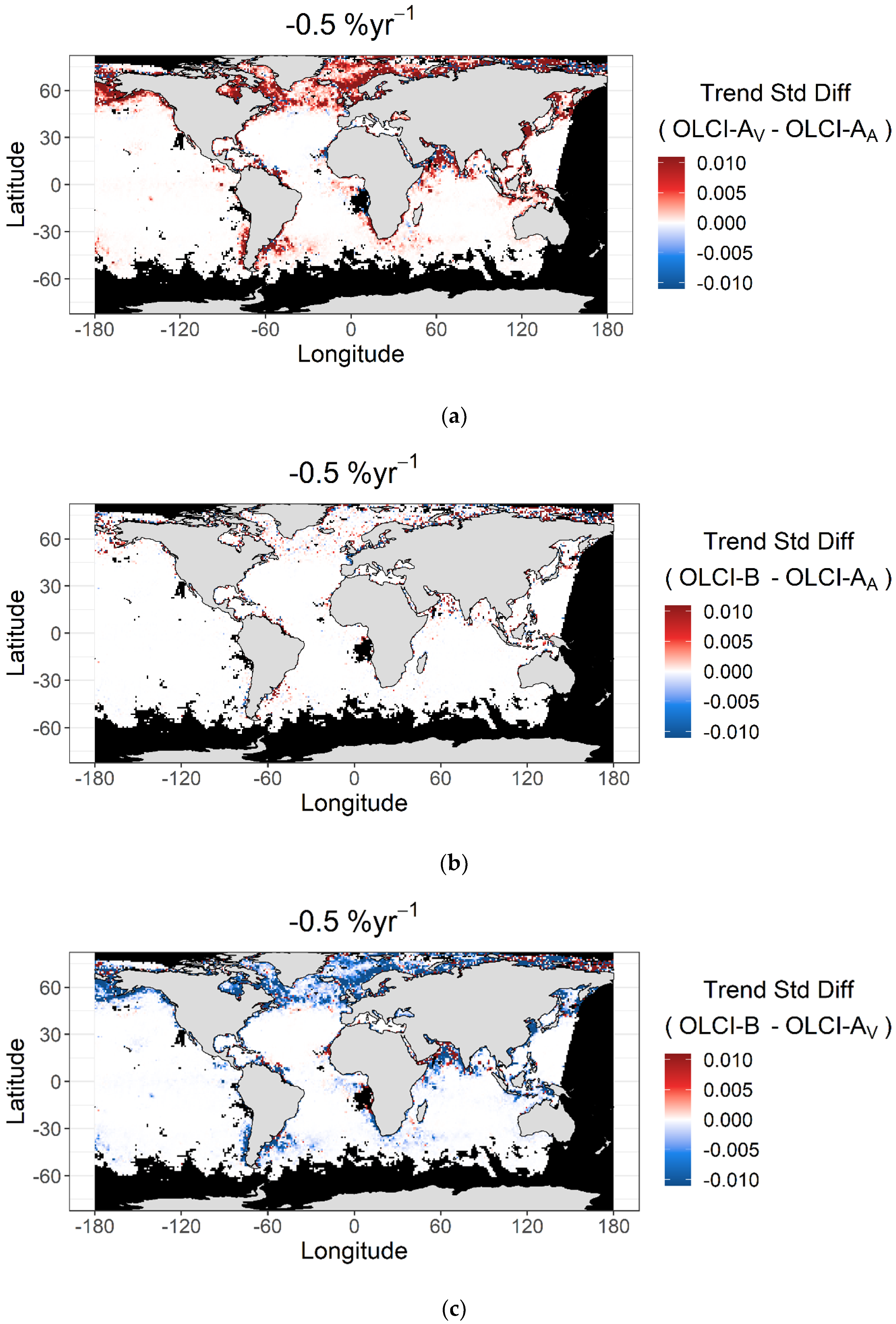
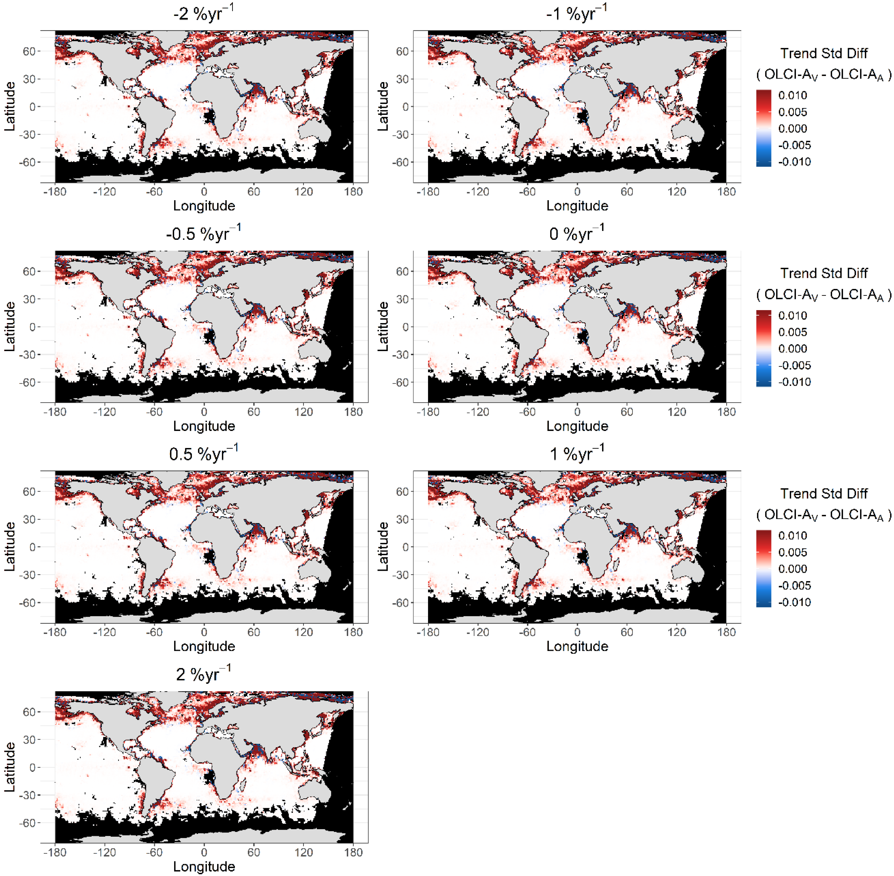
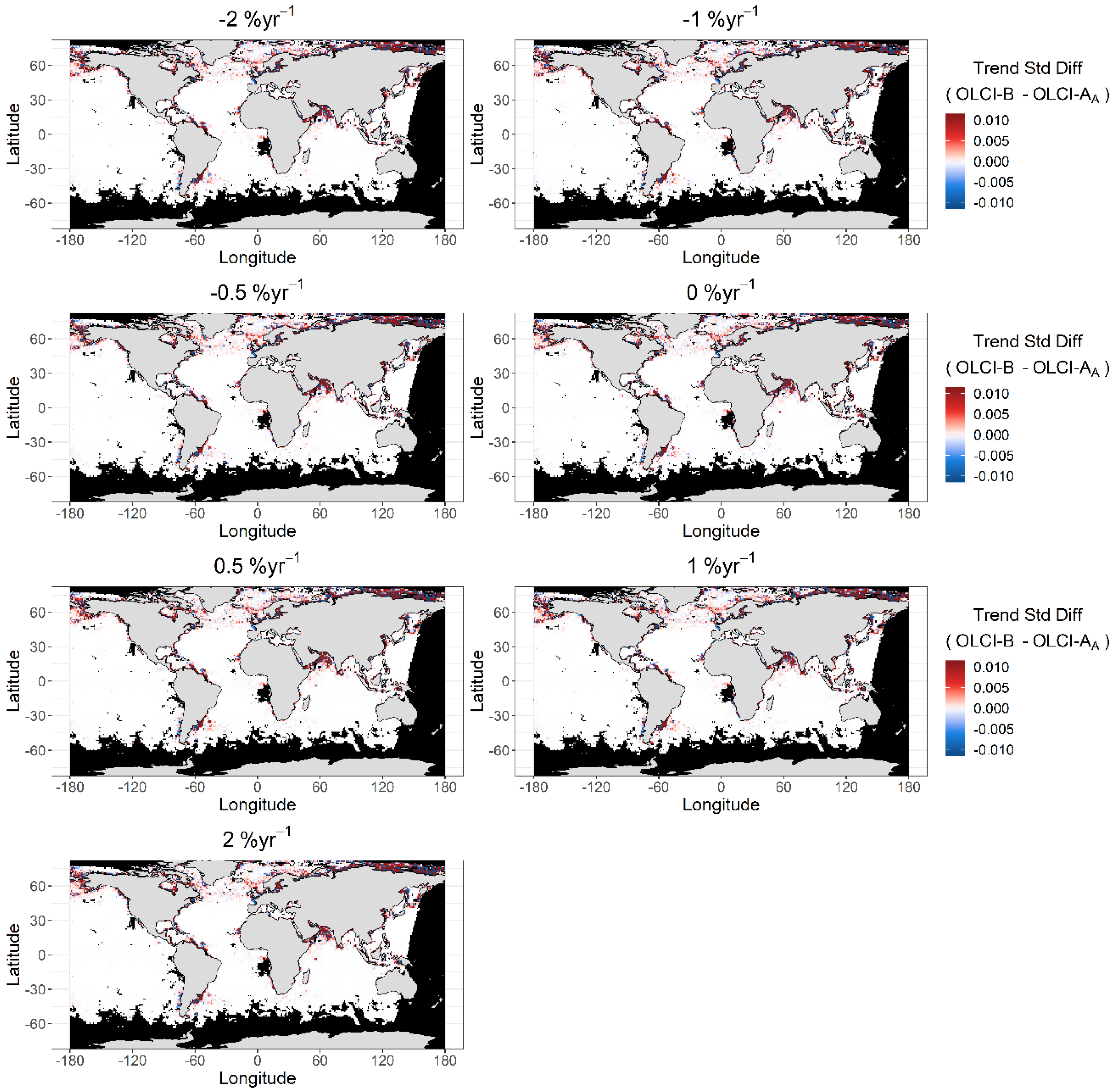
The spatial pattern of differences was also analysed for the same input trend as above (−0.5%·yr⁻¹). In Figure 4, for each grid cell the difference between (a) OLCI-A-Aligned and OLCI-A-Vicarious, (b) OLCI-A-Aligned and OLCI-B, and (c) OLCI-A-Vicarious and OLCI-B was calculated, with a positive value indicating that the latter had a greater standard deviation of chl-a trend estimates than the former. Appendix B shows similar figures at all input trend levels. The overall observation is the same as for the global histograms in that there is a relatively small difference between the datasets. OLCI-A-Vicarious shows more variance of chl-a trend estimates than OLCI-A-Aligned. OLCI-A-Aligned shows more similarity to OLCI-B than OLCI-A-Vicarious, which is expected from how the OLCI-A-Aligned dataset is produced. However, differences are typically small, with 90% of the differences in chl-a trend estimates between OLCI-A-Aligned and OLCI-A-Vicarious in the range ±0.11%·yr⁻¹, ±0.027%·yr⁻¹ for OLCI-A-Aligned and OLCI-B, and ±0.11%·yr⁻¹ for OLCI-A-Vicarious and OLCI-B. By means of the radiometric alignment of OLCI-A to OLCI-B (OLCI-A-Aligned being understood as a “duplicate” of OLCI-B) it is completely consistent to see similar results between OLCI-A-Vicarious against either OLCI-A-Aligned or OLCI-B. Moreover, the differences are expected to be much smaller between OLCI-A-Aligned and OLCI-B.

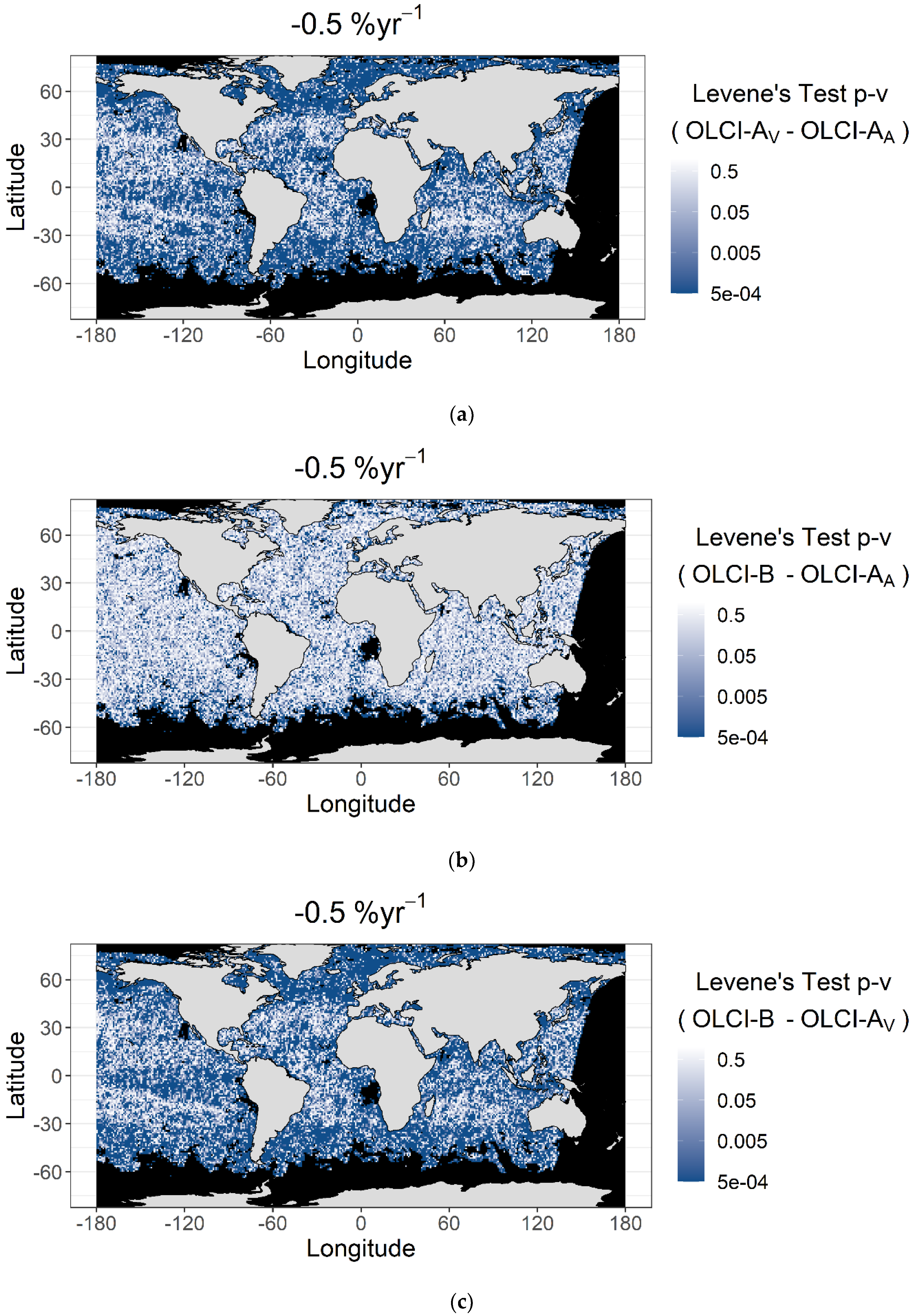
Statistical significance testing (Appendix C) indicates that 70% of grid cells show a significant difference in the variance of chl-a trend estimates between OLCI-A-Aligned and OLCI-A-Vicarious, 29% between OLCI-A-Aligned and OLCI-B, and 71% between OLCI-A-Vicarious and OLCI-B. Appendix C shows that the differences between OLCI-A-Aligned and OLCI-B are typically significant only in randomly scattered points, this anomaly would likely be corrected by using a larger number of bootstraps.

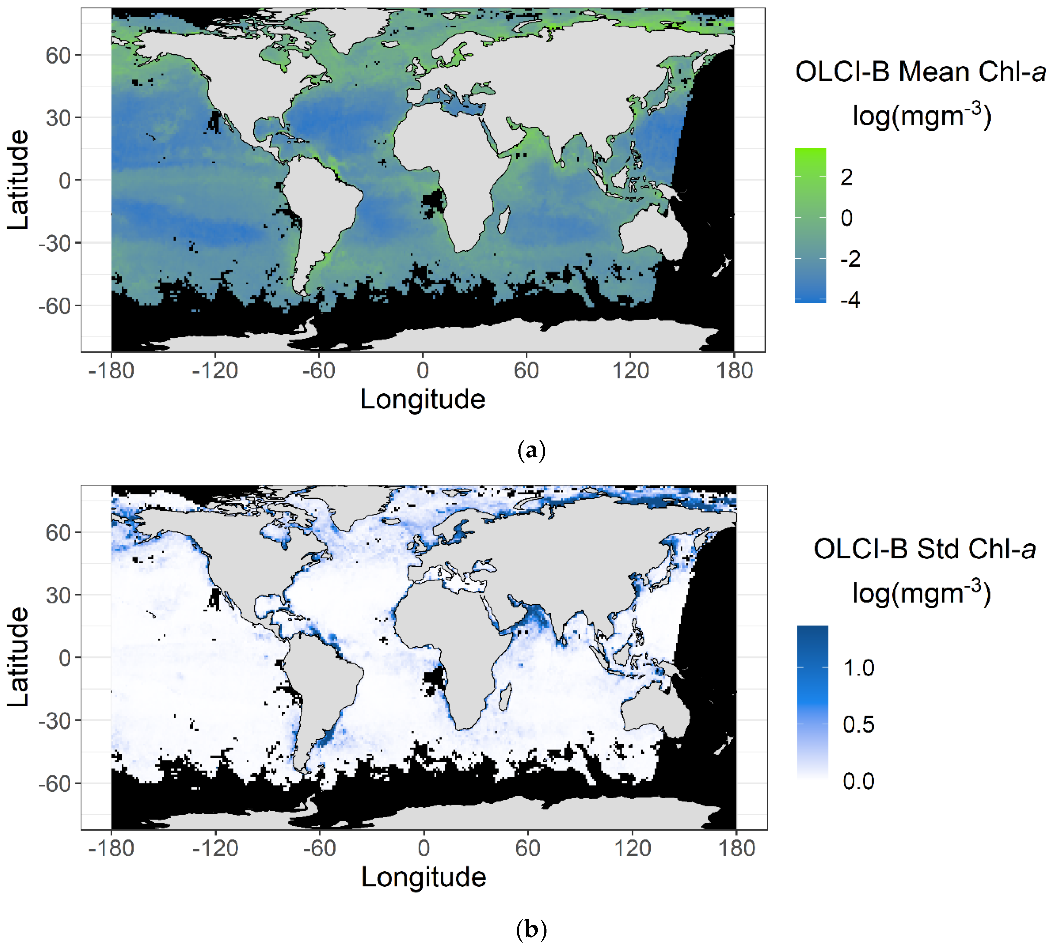
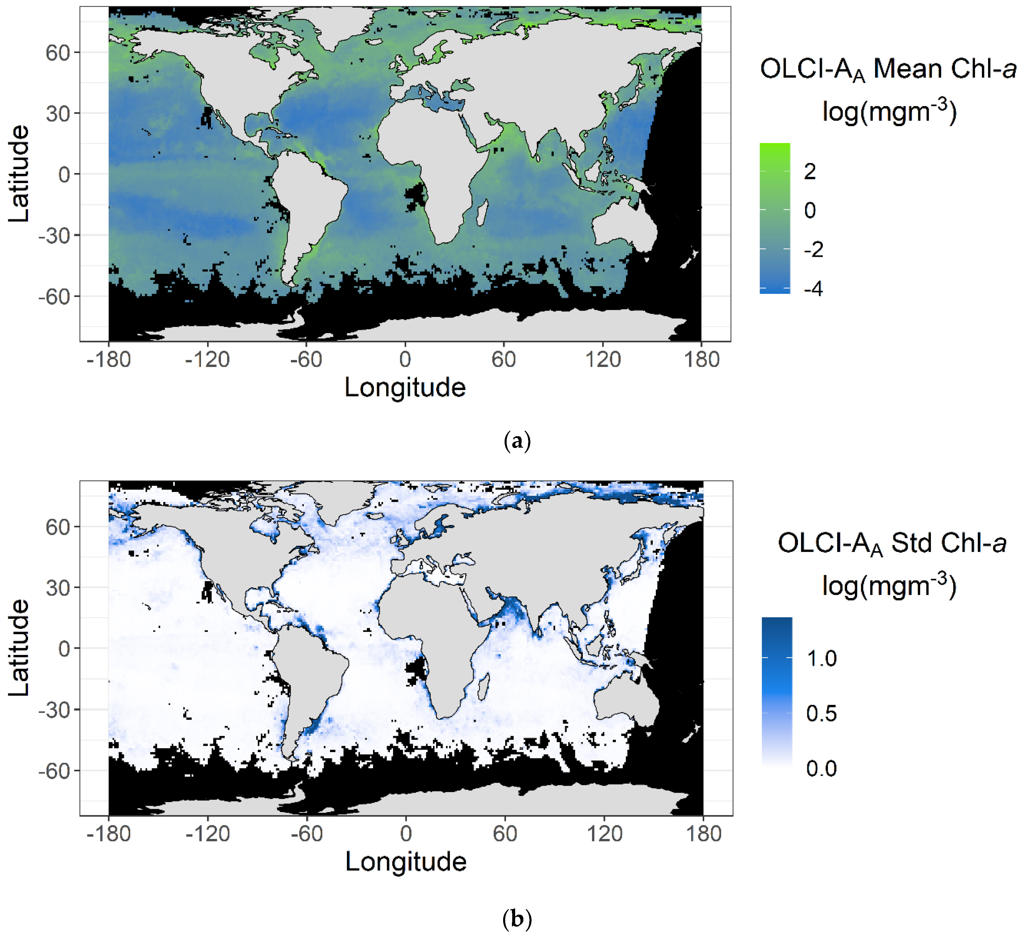
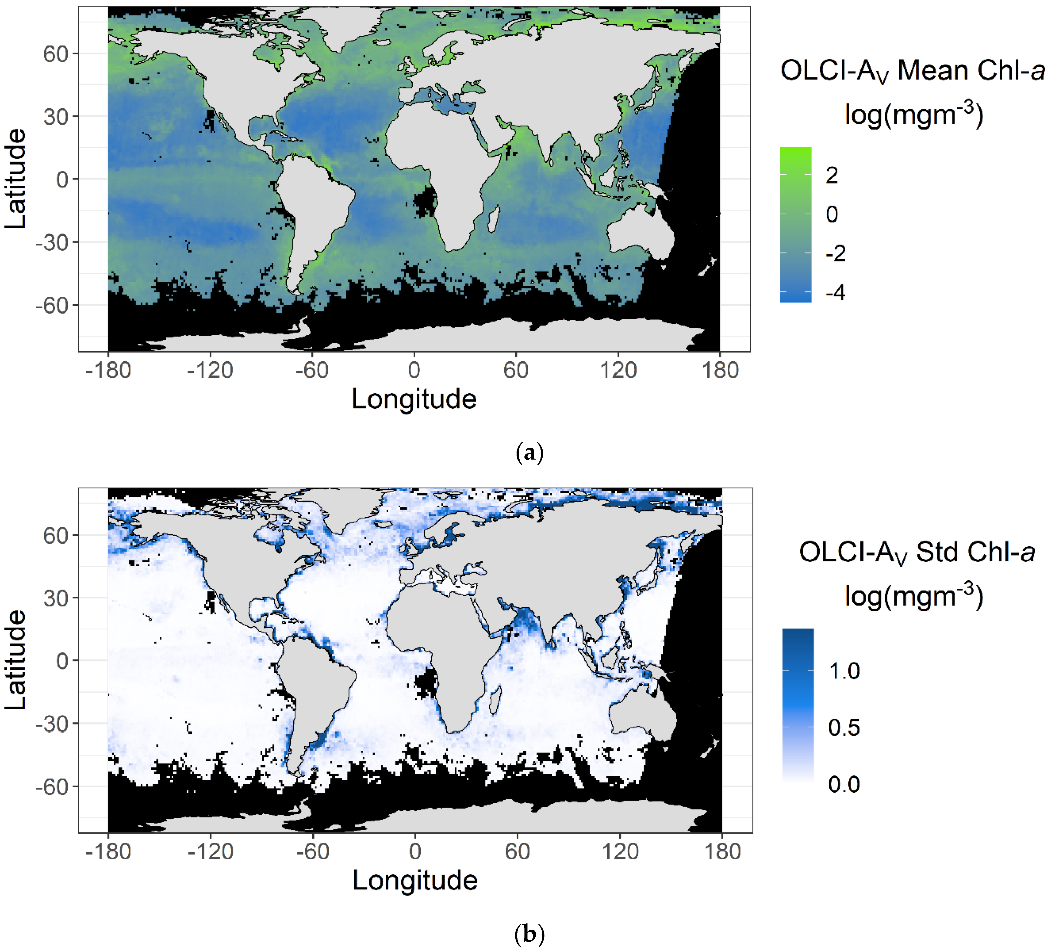
A clear spatial pattern is also seen in the magnitude of this difference, with smaller magnitude differences in the low to mid-latitude open ocean and the largest differences at higher latitudes, particularly in the Northern Hemisphere. This is likely related to the chl-a content itself exhibiting higher dispersion along with higher values (Figure 5). Moreover, fluctuations in the differences in the standard deviation of chl-a trend estimates can be seen, for instance near the coast of the Arabian Peninsula. These can be related to sensitivity of the atmospheric corrections to the relative calibration of the near-infrared bands, as detailed in the methods, such adjustment is performed for OLCI-A Vicarious, as opposed to the other settings. Statistical testing of the differences (Appendix C) shows that OLCI-A-Aligned and OLCI-A-Vicarious are also more likely to have a significant difference in the variance of their chl-a trend estimates at high latitude. It was not possible to complete the analysis in all global ocean grid cells due to missing data from persistent cloud cover, sea ice, low sun angles, and a lack of orbital coverage.

4. Discussion

Whilst there is only a small difference in the variance of chl-a trend estimates between the two aligned sensors (i.e., OLCI-A-Aligned and OLCI-B), it is still important to consider the reasons for the observed spatial pattern. Two factors will underlie this spatial pattern. The first is the actual measurement uncertainty of the two sensors, which may respond differently to different surface and near-surface conditions including contributions from coloured dissolved organic matter (CDOM), total suspended matter (TSM), and other water column constituents, and thus have a spatial pattern. The second factor is the underlying data used as a baseline. Higher latitude data will have more gaps due to an inability to retrieve data during winter because of the low sun angle, plus increased cloud cover throughout the year, known to be increasing due to climate change [22], which will add more degrees of freedom when estimating trends, thus exacerbating any differences in uncertainty between the two sensors. Both are supported by the pattern of differences corresponding to regions of higher chl-a variability—these are expected to have the greatest differences between sensors.

In our analysis, we use a series of globally constant input chl-a trends to assess any impact of trend magnitude on the relationship between estimation and uncertainty. This is in place of a more realistic scenario where chl-a trends vary across the globe [5,7,18,19,20] We find no difference in results for the different input trend levels, indicating that the sensors are affected equally at all the chl-a trend levels analysed, even if a larger trend is shown to lead to a greater variance in trend (Appendix A).

Our analysis assumes that there is no mean difference between the two sensors. A consistent mean difference between two sensors would not be expected to generate differences in chl-a trend estimates from the two sensors. However, potential future sensor ageing may introduce trends in noise or in the mean value of detected chl-a which could potentially impact trend detection if left uncorrected [23]. This is something that will need future monitoring and could potentially be assessed by comparing (in Tandem) future Sentinel-3 OLCI instruments with those already launched and by carefully monitoring the calibration and cross-calibration of the sensors [24].

The Sentinel-3 programme offers sensors of identical design, with frequent platform launches; two satellites are in orbit and two more are planned, each designed with a lifetime of 7 years. However, best estimation of long-term chl-a trends will still include other ocean colour sensors, which will likely be of an alternative design. Because of the different lifespans of sensors, different designs could induce trends in a number of ways. For example, a sensor with more uncertainty at the end of its record is more likely to induce a trend by chance, which may be harder to correct for. For best use of all available ocean colour sensors, projects like the Sentinel-3 tandem phase are advisable between all ocean colour sensors (especially those newly launched), even though this remains a technically challenging prospect.

The differences in uncertainty seen between the two sensors is assumed to arise primarily due to slight remaining calibration residuals, as the temporal difference in the Tandem phase is minimal (~30 s), and only negligible water movement is expected over this timescale. However, other analyses within the OLCI- Tandem project have revealed small quantifiable movements within scenes between OLCI-A and OLCI-B within this time period [14], challenging our assumption. This would have the effect of slightly increasing the differences between estimated OLCI-A and OLCI-B chl-a trends, which are here deemed to be negligibly small.

5. Conclusions

We performed an analysis to understand the effect of sensor uncertainty on estimation of potential chl-a trends in the Sentinel-3A and B OLCI sensors, including two versions of OLCI-A (aligned and vicariously adjusted), using data from the tandem phase. Using multiple synthetic time series with pre-determined chl-a trends, and additional bootstrapping for sensor uncertainty, we re-estimated the trends to understand the effect of sensor uncertainty on trend detection. From this analysis of synthetic chl-a trends, we were able to determine that any differences in uncertainty between the two sensors (and two versions of OLCI-A) will have only a limited effect on chl-a trend estimation. Globally, it can be seen that OLCI-B tends to have a negligibly higher standard deviation of chl-a trend estimates (0.268%·yr⁻¹ for OLCI-B versus 0.266%·yr⁻¹ for OLCI-A-Aligned). OLCI-A-Vicarious has a slightly greater standard deviation, expected from how it is calculated (0.272%·yr⁻¹), but this can still be considered a negligible difference from OLCI-B and OLCI-A-Aligned. There is some spatial variation in the differences, with open ocean regions being the most similar and high northern latitudes and coastal regions being the most different, albeit still with an almost negligible difference. This analysis shows that the effect of differences in sensor uncertainty will only have a negligible impact on future chl-a trend estimation using the Sentinel-3 platforms, where each satellite carries the same sensor design. This analysis does not, however, and cannot, estimate the differences from future drift in sensors, which may well have a significant impact and will need to be monitored. Likewise, differences between past, present, and future non-Sentinel sensors are not considered, even though these differences may have a significant impact on chl-a trend detection, which typically relies on records merged from multiple sensors.

The tandem phase was a unique opportunity to perform this assessment free of temporal differences, and it is strongly advised that this exercise is repeated in future with further Sentinel-3 satellites. It may be even more useful if this could be performed with other ocean colour satellite systems, although a technically challenging prospect. This analysis shows the design strengths of the Sentinel-3 platforms, with quasi-identical sensor design minimising the differences between satellites, allowing a long-term climate data record to be built up without the need for challenging corrections to be applied to compensate for sensor and platform design.