Article

Water Stress Estimation in Vineyards from Aerial SWIR and Multispectral UAV Data

by
Zacharias Kandylakis
,
Alexandros Falagas
,
Christina Karakizi
and
Konstantinos Karantzalos
*
Remote Sensing Lab, National Technical University of Athens, 15780 Athens, Greece
*
Author to whom correspondence should be addressed.
These authors contributed equally to this work.
Remote Sens. 2020, 12(15), 2499; https://doi.org/10.3390/rs12152499
Submission received: 10 July 2020 / Revised: 27 July 2020 / Accepted: 30 July 2020 / Published: 4 August 2020
(This article belongs to the Section Remote Sensing in Agriculture and Vegetation)

Abstract

:
Mapping water stress in vineyards, at the parcel level, is of significant importance for supporting crop management decisions and applying precision agriculture practices. In this paper, a novel methodology based on aerial Shortwave Infrared (SWIR) data is presented, towards the estimation of water stress in vineyards at canopy scale for entire parcels. In particular, aerial broadband spectral data were collected from an integrated SWIR and multispectral instrumentation, onboard an unmanned aerial vehicle (UAV). Concurrently, in-situ leaf stomatal conductance measurements and supplementary data for radiometric and geometric corrections were acquired. A processing pipeline has been designed, developed, and validated, able to execute the required analysis, including data pre-processing, data co-registration, reflectance calibration, canopy extraction and water stress estimation. Experiments were performed at two viticultural regions in Greece, for several vine parcels of four different vine varieties, Sauvignon Blanc, Merlot, Syrah and Xinomavro. The performed qualitative and quantitative assessment indicated that a single model for the estimation of water stress across all studied vine varieties was not able to be established (r2 < 0.30). Relatively high correlation rates (r2 > 0.80) were achieved per variety and per individual variety clone. The overall root mean square error (RMSE) for the estimated canopy water stress was less than 29 mmol m−2 s−1, spanning from no-stress to severe canopy stress levels. Overall, experimental results and validation indicated the quite high potentials of the proposed instrumentation and methodology.

Graphical Abstract

1. Introduction

At a global scale, water demand will significantly increase in the next 30 years [1]. In this context, the EU Common Agricultural Policy reports that 44% of the total water abstraction in Europe is used for agricultural purposes. Thus, managing available water reserves through efficient irrigation practices is crucial, both from an economic and an ecological point of view. In particular, current climate trends elevate the importance of vegetative water stress indicators, in a variety of agricultural zones worldwide, as water demand is on the rise. In high-value crops such as vitis vinifera, management of water stress levels is a widely practiced and very important strategy, to achieve high quality grapes, leading to premium wine products [2], while concurrently reducing the production’s ecological footprint.
Plant water status is associated with various indirect parameters that could be assessed through remote sensing, proximal observations and spectral analysis techniques [3]. The efficient exploitation of all these techniques and observations towards plant water status’ accurate estimation and mapping at parcel scale arises as a challenging task. In most plant species, stomatal closure is affected by several environmental and physiological factors such as light, carbon dioxide concentration, leaf-to-air vapor pressure deficit, leaf/plant water status and abscisic acid [4]. Grapevines, in particular, are considered very sensitive to water stress and even short-term water deficits have been reported to affect growth processes and induce stomatal closure, ending up in an increase in leaf temperature [3]. One of the ways to quantify stomatal closure is stomatal conductance (gs), measured in mmol m−2 s−1, and defined as the rate of passage of carbon dioxide (CO2) entering, or water vapor exiting, through the stomata of a leaf [5].
Satellite data have been employed for estimating vegetation water-stress at medium spatial resolution. In particular, Thermal Infrared (TIR) imagery and hyperspectral data from the Airborne Visible/Infrared Imaging Spectrometer (AVIRIS) have been employed to study thermal variability, showing promising results for broad agricultural analysis [6]. Landsat TM/ETM+ imagery, specifically Near Infrared (NIR) and Shortwave Infrared (SWIR) bands, have been used to estimate water-stress through empirical methods (reflectance trapezoid) [7]. In addition, NIR and Red-Edge bands of WorldView-2 imagery have been correlated with crop/plant/fruit biophysical and biochemical quality parameters in vines, achieving high r2 scores in the range of 0.70–0.95 [8]. Furthermore, comparisons have been made between vegetation water content derived from shortwave-infrared (MODerate resolution Imaging Spectroradiometer, MODIS) and passive-microwave sensors (WindSat) over central Iowa, with the resulting relationship between the two being linear [9]. MODIS evapotranspiration (MOD16) data have been utilized, in novel models, such as the evapotranspiration warning index (ETWI), to study water-stress trends across large cropland regions, on a global scale [10]. On a parcel scale, monitoring of evapotranspiration, as an indicator of water-stress, has been achieved by fusing MOD16 and Landsat data [11]. SWIR data from the Spinning Enhanced Visible and InfraRed Imager (SEVIRI) have also been proven very useful, in the evaluation of canopy water stress in the Senegal River basin, a semi-arid zone of mainly savanna and grassland [12].
For vegetation mapping tasks at high spatial resolutions, recent advances in sensor technology have made available compact sensors, which can be utilized in custom unmanned aerial vehicle (UAV) solutions, along with single-board computers, opening up a wide array of possibilities in precision agriculture applications like water management in viticulture. The areas covered by UAV flights, combined with the achieved pixel sizes and the cost efficiency of this approach, qualify it as particularly useful for the canopy scale study of vineyards [13,14]. As for proximate sensing viticultural studies, many research efforts have employed TIR sensors towards estimating leaf water content at different spatial scales, mainly through the computation of the Crop Water Stress Index (CWSI) [15]. This approach requires the measurement of dry and wet temperatures on leaf/canopy as reference for the normalization in CWSI calculations. In recent relevant works, the correlation between CWSI calculated using airborne UAV thermal sensors’ data, and CWSI calculated utilizing proximal thermal sensors’ data, has been established for vineyards, with standard errors ranging from 2–12% [3]. Additionally, the stable linear relationship (r2 in the range of 0.63–0.91) between CWSI, calculated from thermal imaging sensors’ data and leaf stomatal conductance (gs) in Merlot vineyards, has been presented, highlighting the need for further required research for individual varieties [16]. A different method, for the estimation of root-zone soil moisture in willow short rotation coppice, was proposed by Wang et al. [17], using a temperature–vegetation triangle approach combining UAV visible, multispectral and TIR data. By also incorporating surface roughness in their model, they achieved r2 rates of 0.69 for the estimation of soil moisture at a 15–30 cm depth.
Beyond thermal imaging and proximate in-situ sampling, recent studies highlighted the relation between canopy water stress and SWIR observations. In particular, concrete correlations were established with SWIR observations, in a laboratory environment for eleven tree species (e.g., European Beech, Norway Maple), at leaf scale for tomato plants, and at single plant canopy scale for potted potato plants [18,19,20]. However, due to the relatively new, bulky, heavy, energy-demanding instrumentation as well as its challenging integration and processing configurations, airborne sensors have rarely been employed and investigated for estimating water status at canopy scale, for the entire grapevine, or for other crop parcels. Specifically, UAV-mountable Indium Gallium Arsenide (InGaAs) detector technology is fairly recent and has intriguing potential for precision viticulture. Furthermore, González-Fernández et al. [21] identified with a field spectrometer that the spectral band centered around 1450 nm (SWIR spectrum) was the most suitable data to estimate leaf water content in vineyards for the varieties Mencía, Cabernet Sauvignon, Tempranillo and Merlot. Rapaport et al. [22], also using a portable spectrometer, comprehensively studied proximate observations for water stress status. Their proposed vine-specific indices for water status estimation indicated that wavelengths around 1485–1500 nm (SWIR spectrum) emerge as the most significant. Beyond grapevines, for eleven tree species, Ullah et al. [18]’s findings indicated that SWIR data were also the most valuable for water stress estimation among visible/near-infrared (VNIR), SWIR, mid-infrared (MIR) and TIR data.
In addition, experiments in a greenhouse, under a controlled irrigation setting, examined the correlation between potato leaf stomatal conductance, measured with a leaf porometer, and reflectance from broadband, hyperspectral thermal sensors and VNIR/SWIR spectrometers. The fastest responders to water-stress were CWSI and NIR/SWIR-based indices [19]. Furthermore, a recent study focused on the discrimination of abiotic (water-stress) and biotic (root-knot nematode infestation) stress in tomato plants under controlled irrigation and infestation settings. Based on hyperspectral data and Support Vector Machines (SVM) for the classification procedure, the results indicated that the reflectance at 1500 nm (SWIR spectrum) was strongly linked with water-stress levels without showing strong correlations with biotic stress [20]. This was an important observation, which possibly differentiates the application perspectives of thermal and SWIR imaging.
Despite the aforementioned findings, which indicated the quite high potentials of SWIR data for water stress estimation at leaf and canopy scales, SWIR sensors onboard aerial vehicles have not been adequately exploited and assessed towards this goal. Still, their potential in estimating and mapping water stress at very-high resolution (<1 m) is rather unexplored. At the same time, such a mapping solution is of significant importance for a number of viticultural practices including vineyard management, control and monitoring of maturity, phenolics and sugar content.
To this end, in this paper we propose a novel aerial SWIR-based instrumentation and processing methodology for estimating water stress in vineyards at canopy level. In particular, we have designed, developed and validated an unmanned aerial SWIR and multispectral data acquisition system. In addition, we examined, through data analytics and modeling procedures, the relations that could be established between the acquired aerial imaging data and water stress at grapevine canopy scale. Beyond the hardware integration tasks, we have developed a novel methodology towards water stress mapping. Experiments were performed in two viticultural regions in Greece, on six different parcels of four vine varieties, namely Xinomavro, Merlot, Syrah and Sauvignon Blanc. To the extent of our knowledge, no other study up to now has presented such an aerial multispectral and SWIR instrumentation, methodology and assessment highlighting the quite powerful potential of water stress mapping in vineyards under the developed framework.

2. Materials and Methods

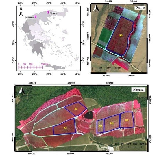
2.1. Study Areas, Vineyards and Vine Varieties

Data acquisition campaigns were conducted in two important viticultural regions of Northern Greece, namely Drama and Naousa, belonging to local Protected Geographical Indication (PGI) and Protected Designation of Origin (PDO) zones of the same name, respectively. The specific locations of these areas are presented in Figure 1a, over an administrative map of Greece. Concurrent field measurements and UAV flights were performed during the veraison period, in late July of 2017.
The first study area, Drama, is located in Eastern Macedonia and Thrace, an administrative region of northern Greece. The field campaigns were applied on a Sauvignon Blanc vine parcel of about 2 ha, located near Kali Vrisi village, at an altitude of 210 m above sea level. This parcel is presented in Figure 1b and for the sake of brevity, shall be henceforth referred to as SB.
The second study area, Naousa, is located in Central Macedonia, Greece, inside the PDO zone Naousa. Originating in this zone is Xinomavro, the most promising Greek red wine variety, which has contributed extensively to the recent surge in popularity and amelioration of Greek wine status abroad. Our field campaigns were conducted at a plateau of about 200 m altitude, near the Giannakochori village. Data were acquired for five vine parcels of the Xinomavro, Merlot and Syrah varieties, covering an area of about 6 ha. The two Xinomavro parcels studied belong to different clones of the indigenous variety, namely V1 and V3, whereas the two Merlot vineyards belong to the same clone. They shall be henceforth named as X1, X2, M1 and M2, respectively, while the Syrah vineyard studied shall be referred to as SY. The outlines of these parcels can be observed in Figure 1c.

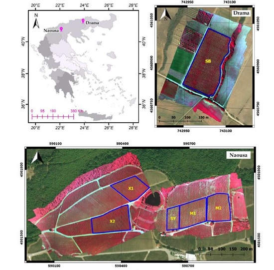
2.2. Field Campaigns

Field campaigns were conducted on 26 July 2017 and 29 July 2017 for the Drama and Naousa regions, respectively. Climatological data for July, from the nearest meteorological stations to the study areas are provided in Table A1, Table A2 and Figure A1. For both study areas, in-situ data were acquired, namely leaf porometer observations along with their exact GPS location measurements. Concurrently, with a maximum time-difference of 30 min, a SWIR and a multispectral sensor, on-board a multicopter UAV, captured imagery data for the studied parcels. Radiometric calibration panels were placed around and inside the vineyards and ground control points (GCPs) and were also marked and measured with a Real-Time Kinematic Global Positioning System (RTK GPS) instrument. In Figure 2, instances from the different aspects of the field campaigns at the Drama and Naousa study areas are presented.

2.2.1. Leaf Porometer and GPS Field Measurements

Regarding field measurements, leaf stomatal conductance (gs) in units of mmol m−2 s−1 was measured at midday with a leaf porometer (SC1-Leaf Porometer, Decagon Devices Inc.). The leaves chosen for measurement adhered to some specific conditions. First of all, they were located at the top of the canopy, so that their reflective properties were observable in the concurrent imagery. Furthermore, they were mature leaves of average size, representative of the current vine-plant and exhibiting no sign of pathogens. To validate the data acquisition process, every measurement was taken twice. If the indications had a percentile difference of more than 15%, the measurement was repeated for a third time. The closest two indications for each leaf were averaged. The subsequent result was recorded as the stomatal conductance of that in-situ data acquisition point. Stomatal conductance is the degree of stomatal opening related to leaf water potential (ΨL) by feedback processes and can be used as an indicator of plant water status.
Concurrently, the geolocation coordinates (X, Y) on the projected coordinate system of Greece (GGRS87) for each point were measured using an RTK GPS (Ashtech ProMark 200 GPS L1/L2 RTK Rover). To ensure a geolocation accuracy better than 15 cm, X, Y coordinates of each point were measured for at least one minute.
In Figure 3, the distribution of in-situ data acquisition points for each parcel can be observed, overlaid on the extracted canopy. In total, 104 points were measured for both study areas. For the first one, Drama, stomatal conductance with exact geolocation was measured at 47 points for parcel SB, with values in the range of 58–245 mmol m−2 s−1. We should note here that 2 points were considered statistical outliers for this parcel, since their values were higher than 700 mmol m−2 s−1. In the second study area, Naousa, the measurements acquired were 9 for X1, 11 for X2, 12 for M1, 16 for M2 and 9 for SY. The respective ranges in mmol m−2 s−1 were 75–214 for X1, 75–389 for X2, 272–770 for M1, 165–783 for M2 and 142–497 for SY.
In the Drama study area, for parcel SB, in situ measurements were acquired to estimate the Leaf Area Index (LAI), which is the ratio of total one-sided area of leaf tissue per unit of ground surface. LAI is a physiological property that quantifies canopy density and serves as an index of vine vigor and subsequently yield [23,24]. It is an important tool for vine growers, supporting their decision-making process. For six vines throughout the parcel, the total number of leaves per vine were counted, as well as indicative measurements, to calculate an average leaf area per vine. The Total Leaf Area per vine was calculated as the product of the number of leaves by the average leaf area. In addition, vine width (VW), vine length (VL) as well as row spacing (RS), were measured. LAI was then empirically calculated for those six vines using (1).
LAIin-situ = (Total Leaf Area)/(VW × VL × RS)

2.2.2. UAV Imagery Acquisition

The imagery data was acquired with two sensors mounted on a custom-made UAV multicopter solution. The multispectral sensor employed was a Parrot Sequoia sensor, with a resolution of 1280 by 960 pixels and four available bands, targeting vegetation applications (green: 530–570 nm; red: 640–680 nm; red edge: 730–740 nm; and NIR: 770–810 nm). It was accompanied by a sunshine sensor and calibration panel, to adjust for different irradiance conditions. SWIR data was acquired with a Xenics Bobcat 640 GigE camera, based on a temperature-stabilized InGaAs detector. This SWIR single-band video sensor is sensitive in the 900–1700 nm range and has a resolution of 640 by 512 pixels, a focal length of 25 nm and an effective framerate of 4 fps. The sensor had an Ethernet interface and was connected onboard to a single board custom-made lightweight mini-ITX computer, for real-time SWIR and ancillary data acquisition and storage.
For the study area of Drama, a single flight was conducted to acquire imagery data for parcel SB. Two flights were conducted in the study area of Naousa, over the X1, X2 and SY, M1, M2 vine parcels. The flight altitude was in the range of 80–100 m in all cases. The speed of the UAV was set at 3 m/s to achieve high front overlap of at least 80% for both sensors, and the distance between the flight rows was arranged so as to achieve a side overlap of at least 80%.
To ensure the accuracy and validity of the georectification process, 6–8 GCPs were designated. This was achieved by placing portable targets on the field or by marking points that could be precisely pinpointed in the imagery. Accordingly, the use of 8 custom-made reflectance panels, of oblong rectangular shape, made of materials with relatively high Lambertian reflectance properties, allowed the subsequent reflectance calibration of the imagery data. The positions of both GCPs and calibration panels were measured for at least one minute using RTK GPS.

2.3. Methodology Framework

The designed, developed and validated methodology towards water stress mapping is outlined in Scheme 1. Upon the aerial data acquisition, both multispectral and SWIR data were processed through standard Structure-from-Motion (SfM) and Multi-View Stereo (MVS) procedures. From these procedures, the SWIR and multispectral orthoimages were derived. These two datasets were then co-registered and were geometrically aligned with sub-pixel accuracy. Following that, reflectance values were calculated based on the observations from the radiometric calibration boards. Subsequently, the imagery was clipped at parcel scale and resulted in the Analysis-Ready Multispectral and SWIR Data (ARD).
From the ARD, various spectral indices were calculated. Then, the canopy was detected based on Normalized Difference Vegetation Index (NDVI) thresholding, along with simple per-parcel segmentation and manual correction when required. For the modeling procedures, pixels from canopy SWIR reflectance data were employed and correlations were examined against the in-situ data. Geospatial maps indicating water stress levels (mmol m−2 s−1) were derived and an additional visualization and per vine row estimation and assessment was computed.

2.3.1. Co-Registration and Reflectance Calibration

Initially, pre-processed image data was ingested using a commercial software (Agisoft, version 1.2.5) executing Structure From Motion (SfM) and Multi-View-Stereo (MVS) towards Digital Surface Model (DSM) and orthoimage production per image modality. The georectification process required the annotation of the 6–8 GCPs per flight, and the insertion of their measured coordinates. In addition, utilizing the extracted canopy and the DSM, Digital Elevation Models (DEM), as well as the respective slope and aspect data, were computed.
The orthoimages produced from the aforementioned procedure, despite the employment of the same GCPs, were not perfectly aligned (left, Figure A2) mainly due to underlying terrain relief and high-resolution data. A co-registration procedure followed, based on an affine transformation, which adequately recovers the geometry of the multispectral orthoimage, to match the geometry of the SWIR one. In Figure A2, an indicative case of the initial misalignment is shown, where the green color is the detected canopy on the SWIR data, and the red is the canopy on the multispectral data. It can be observed that several mis-registration cases had occurred (left, Figure A2), while after the co-registration, both datasets are aligned with sub-pixel accuracy.
In the next step, scene reflectance was generated. For the SWIR dataset, an image calibration process was executed, based on an empirical approach, by exploiting the observed radiometric reference panels. These panels were custom-made and were measured in the laboratory with a portable spectroradiometer indicating an acceptable flat spectral response. The considered airborne campaigns were performed under stable atmospheric conditions over all sites and, moreover, the deployment of several reference panels described the calculated uncertainties. It should be pointed out that two panels were not exploited on the calibration process and were used to validate the derived reflectance values. Although the multispectral data were calibrated based on incident irradiance measured during flight by the camera’s integrated sensor, a similar empirical approach was additionally followed in order to cross-validate the result. It should be noted that more advanced reflectance generation approaches [25] including reflectance anisotropy removal due to topography, bidirectional reflectance distribution function and shadows were not performed and their examination were beyond the scope of this work. In order to produce the Analysis-Ready Data (Scheme 1, Figure 4), SWIR and multispectral reflectance orthoimages were clipped at parcel scale.

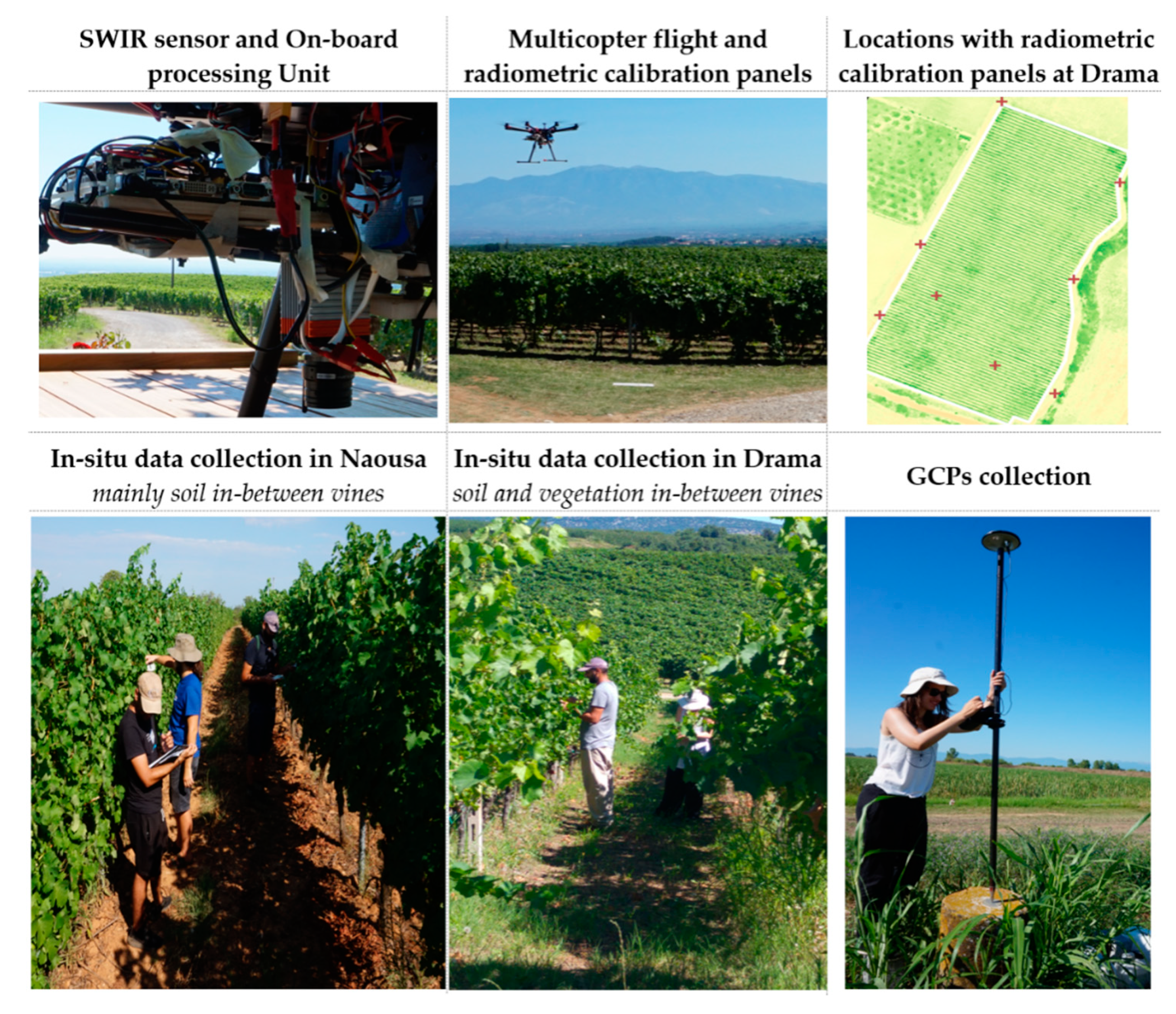
2.3.2. Spectral Indices and Canopy Extraction

In order to detect the canopy per parcel, NDVI, as proposed by Tucker et al. [26], was computed. A standard thresholding segmentation approach was followed based on NDVI, which has been proven useful [27] for discriminating between canopy and non-canopy materials, including bare soil, shadows, and inter-row vegetation. For each parcel, a different threshold was chosen to result in a binary canopy raster, while a manual correction step was followed where necessary.
The extracted canopy superimposed on the SWIR data is showcased in Figure 5 (left) for the indicative parcel SB, while Figure 3 also presents the extracted canopy for all considered parcels. Moreover, LAI estimation was also performed, which is related to multispectral observations [28], following the simple empirical approach of Johnson et al. [29] specifically proposed for vineyards, and by applying a linear equation that correlates LAI and NDVI values (2).
LAIJohnson = 4.9 × NDVI − 0.46
This estimation was then cross-checked with in-situ LAI measurements for 6 vine-plants in parcel SB. To reference the same scale, LAIJohnson per vine was calculated by averaging all pixels belonging to that vine. The resulting r2 score was 0.73, indicating a strong correlation between the values estimated by (2) and in situ measurements for LAI computed with (1).

2.3.3. Water Stress Modeling and Mapping

The next step was to aggregate the GCPs geolocation and in-situ stomatal conductance measurements, resulting in vector point data, ready for the modelling process. In a similar work, where correlations were evaluated between image pixels and point measurements, it was reported that the minimum spatial resolution, requisite for such analysis, is 0.3 m [30]. In addition, Gonzaled-Dugo et al. suggested that, to fulfill the relevant viticultural need for water-stress monitoring, it is necessary to study pure canopy pixels, avoiding mixed soil/vegetation pixels [31]. Thus, the scalability of this study from leaf to canopy is established by achieving the above-stated requirements. Additionally, as mentioned in the Section 2, leaf selection was representative of the respective vine-plant.
Using the gs vector point data and the extracted canopy for SWIR data, an automated statistical analysis was performed in Python. Linear and exponential regression models were calculated, to establish correlations between in-situ data for stomatal conductance (point measurement) and SWIR reflectance (pixel value). Further experiments were also performed, in order to examine if this correlation was robust and the leaf/point measurement could be scalable to one or several vine-plants/pixels. More specifically, for each point measurement, the reflectance of the respective central pixel and all adjacent to it were averaged. This average value was then correlated to the stomatal conductance measurement. The resulting models will be referred to as the 9-pixels neighborhood models, as that was the number of pixels used per point, in most cases. Since the central pixels could be situated near the canopy edges, pixels that were not pure canopy were excluded from the analysis.
Regarding the regression models, a number of different experiments were performed. Although all parcels were subject to different management practices and irrigation treatments, attempts to establish correlations were made both for the entirety of the observations, as well as for each individual parcel. Thus, to refer to the different models, the same nomenclature as for the parcels was used. Additionally, for parcels of the same variety, joint models were also computed, and will be referred to as a conjugation of the relevant parcel names; for Merlot, M1&M2 and for Xinomavro, X1&X2 (note that X1 and X2 represent two different clones from the same variety). To summarize, the computed models were 32. More specifically, for each of the 8 parcels or parcel combinations (M1, M2, M1&M2, SB, SY, X1, X2, X1&X2), four models were calculated, linear/exponential with SWIR value taken from one pixel, the central one relative to the in-situ measurement coordinates, and linear/exponential with sampling of the SWIR values from a 9-pixels neighborhood.
After analyzing the above results, a single model was proposed for each vine parcel studied. The extracted canopy for SWIR data was fed as input to the proposed models, to produce the respective geospatial water-stress maps for each parcel. This intermediate result, for parcel SB, can be observed in Figure 6a. It is easily observable that the width of the studied canopy is small compared to the inter-row distances. To ameliorate the end-product readability from viticulturists, the need for additional visualizations arose. For each vine parcel, the produced water-stress map was rotated so that the lines appeared horizontal. Then, the number of lines was counted, and for each line a new map-product, which is referred to as synthetic representation, was produced. The width of the vine-rows, as well as the distance between them, have been purposefully modified to facilitate visual inspection of the product. In addition, the values included in the synthetic representation are, for each vine-row, per-column medians. An example of how this was achieved is showcased in Figure 6.
In Figure 6b, the data presented is part of the geospatial water-stress map, after rotation. Per vine-line, a sliding vector (black outline) was applied to each column of the rotated water-stress map. The function of this sliding vector was to compute the median value of the included pixels. In Figure 6c, the corresponding sliding vector is outlined for the final water-stress synthetic representation. The values included in the sliding vector are the median values of the corresponding vector of Figure 6b. An additional benefit of this approach, beyond a more efficient and exploitable visualization, is that the possibly mixed pixels on the edges of the canopy are not influencing the final product. Relationships were also explored between stomatal conductance measurements and the derived LAI and DEM slope and aspect for the whole dataset and for different varieties/parcels.

3. Experimental Results and Discussion

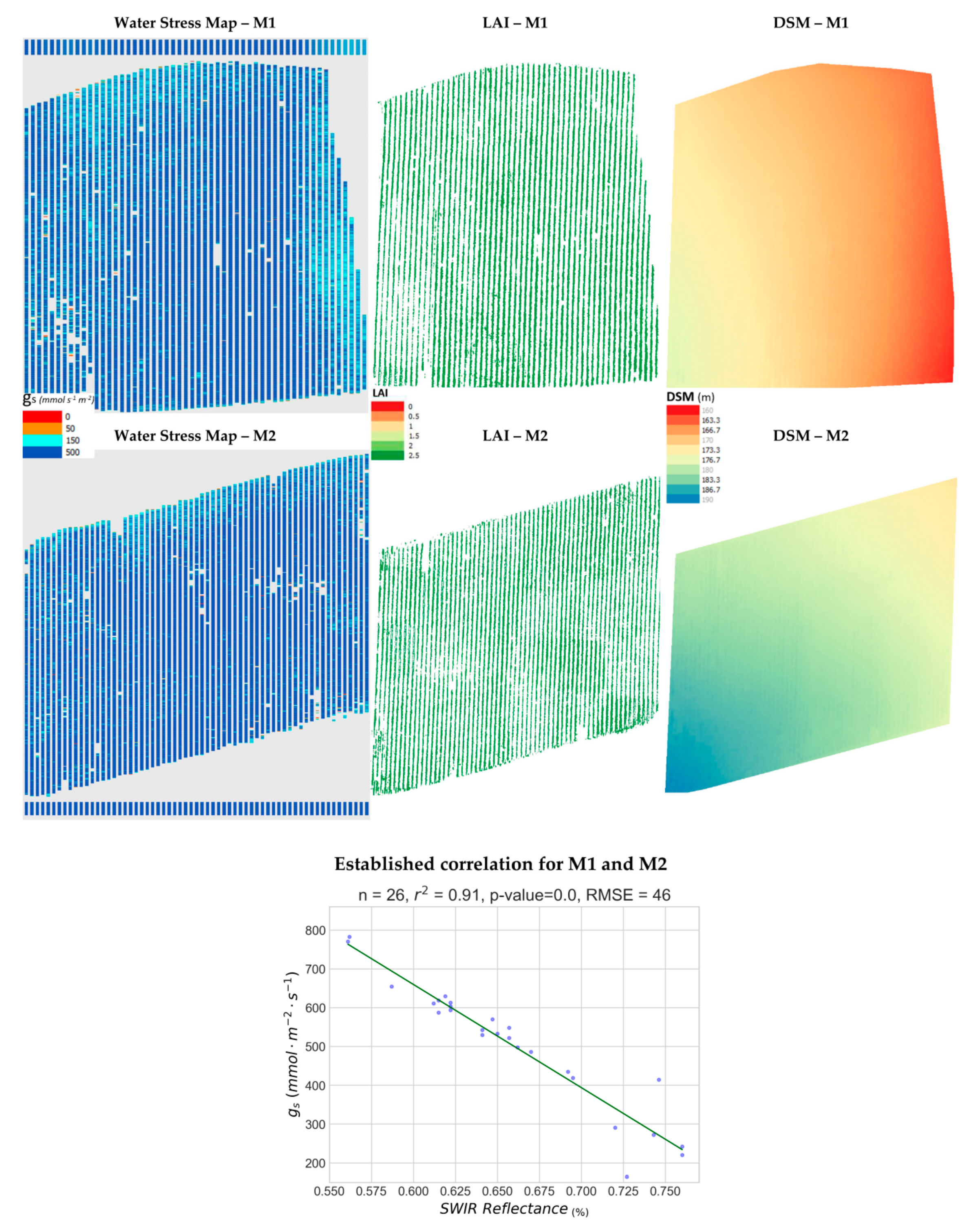
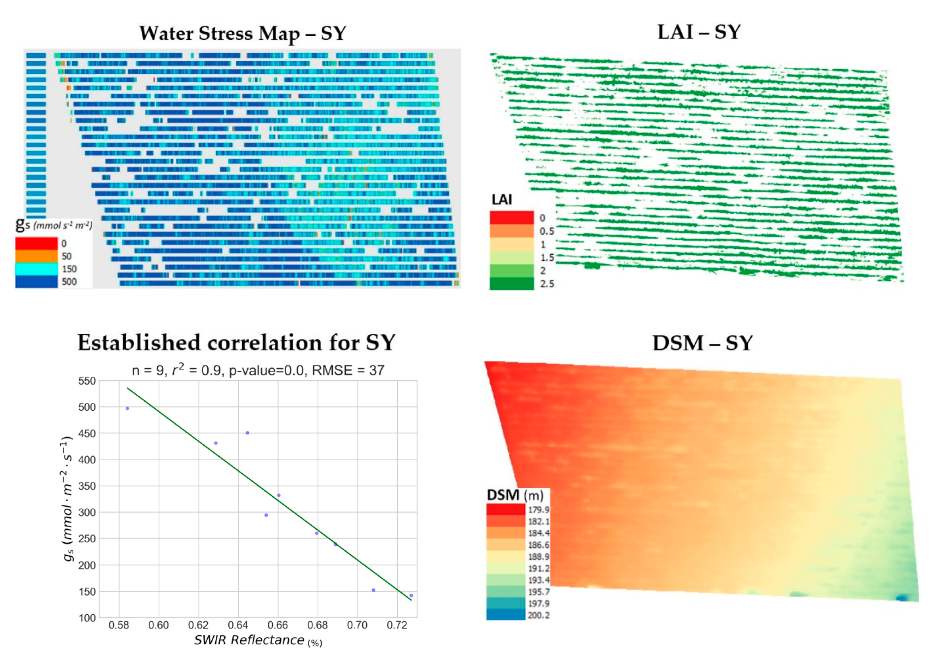
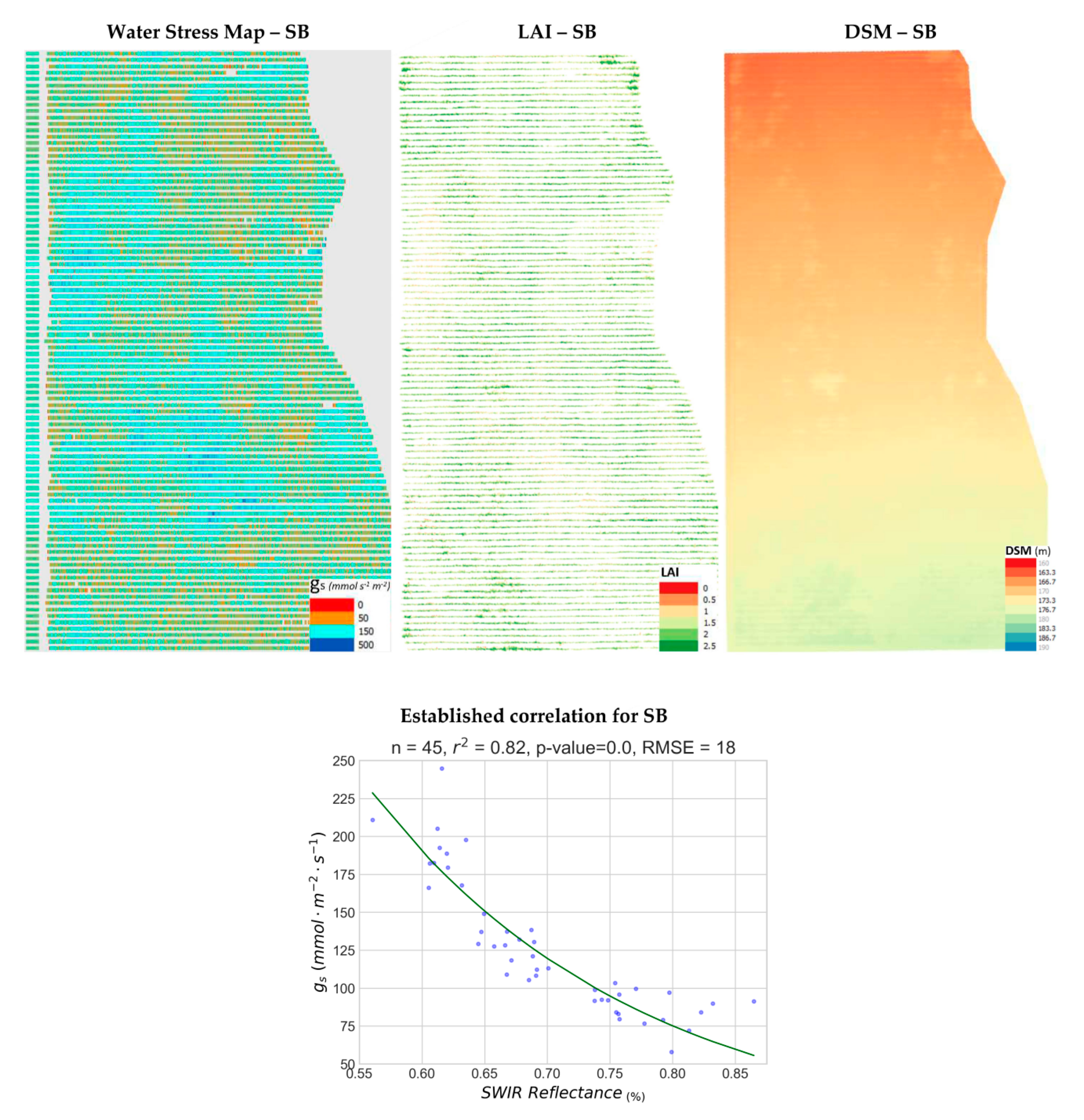
3.1. Regression Results

In this subsection, the results from the produced regression models, between stomatal conductance measurements and SWIR reflectance values, are presented for all experiments applied on the studied vine parcels.
The results of the 32 different models can be observed in Table 1. The sampling of the SWIR reflectance values was taken from one pixel, the central one, relative to the in-situ sampling coordinates. In addition, the same experiments were repeated while sampling the SWIR values from the 9-pixels neighborhood, as long as those pixels were part of the canopy. Quantitative evaluation metrics e.g., r2, root mean squared error (RMSE), and normalized RMSE (NRMSE) for the established correlations, are provided. NRMSE per experiment was computed as the fraction between RMSE value and mean gs value.
The initial experiments included all studied parcels and no correlations were able to be established between all SWIR observations and in-situ data (r2 < 0.30). An indicative attempt to correlate these two datasets is presented in Figure A3. It was priorly known, from the agronomists managing the studied vineyards, that the management procedures and irrigation treatments were different across all parcels. Moreover, different varieties and clones may exhibit differences in hydraulic architecture as well as reflect differently across the spectrum [32,33]. Regarding the 32 experiments with the individual varieties and clones (for X1 and X2), the overall quantitative assessment (both per parcel and per variety models) indicated relatively high correlations (r2 > 0.60 for the linear models) apart from the experiment with the two clones of Xinomavro and a few exponential models.
For the two Merlot parcels, both models (M1, M2) attained regression rates of over 0.90 for the single pixel linear and exponential models. In particular, model M1 achieved r2 scores of 0.91, for both fittings, while the results were slightly better for M2, with r2 scores of 0.95 (linear) and 0.93 (exponential). For the joint model M1&M2, the correlations established had an r2 score of 0.91 (linear) and 0.89 (exponential). The repetition of the experiments, after sampling SWIR values from the 9-pixels neighborhood of each pixel, yielded significantly worse results for M1, presenting drops of over 0.25 for both fitting cases. M2 and joint M1&M2 models also presented lower rates for the 9-pixels neighborhood experiments, but still held scores of 0.86 and 0.74, respectively, when applying the linear regression fitting. RMSE values for these models were in the range of 36–86 mmol m−2 s−1, some of the highest values for all experiments, however as a fraction of the mean gs value, NRMSE exhibits some of its’ lowest values, 0.07–0.18.
For parcel SB, which had the largest number (45) of in-situ observations, the r2 scores were 0.75 for the linear model and 0.82 for the exponential one. RMSE scores were in the range of 18–29 mmol m−2 s−1 and NRMSE in the range of 0.14–0.23. A higher regression score for the exponential model compared to linear, i.e., 0.76 to 0.66, respectively, was also recorded for the SB 9-pixels neighborhood model, hardening the robustness of this fitting for this parcel/variety. Contrariwise, parcel SY exhibited the highest r2 scores of 0.90 for the linear and 0.83 for the exponential model. The neighborhood sampling set-up delivered deteriorated scores, around 0.78 for linear and exponential cases. This may be attributed to the fact that the sampling points were few for this particular parcel and at the same time it had a narrower canopy resulting in a lower number of values for those experiments, since pixels that were part of the neighborhood but not part of the canopy were not taken into account in the average estimation. Although RMSE values seem large for parcel SY (37–64 mmol m−2 s−1), normalization by the mean provides a better indication, with NRMSE percentages in the range of 0.12–0.21.
Xinomavro model X1 achieved r2 scores of 0.83 in both cases (linear and exponential fitting). The second Xinomavro parcel X2, exhibited even better results of 0.96 and 0.92, respectively. For the joint model, the correlations established were significantly worse, with r2 scores of 0.66 and 0.61, respectively. This can be attributed to the fact that the two parcels belong to a different clone of the Xinomavro variety with known different behaviors. The neighborhood sampling set-up significantly decreased scores for both fittings of the X1 model, while X2 presented relative robustness, holding the regression rates at 0.85 and 0.70, respectively. For the joint model X1&X2, r2 scores were above 0.60 for single pixel sampling and relatively lower for the neighborhood sampling. RMSE and NRMSE values further support the exclusion of model X1&X2. It showcased the worst NRMSE of all experiments in the range of 0.30–0.43 of the mean gs value. The proposed linear models for X1 and X2 exhibited similar RMSE of 18 and 21 mmol m−2 s−1, however NRMSE showcases that the error as a fraction of the respective mean value is 0.05 lower for X2.
The correlations between stomatal conductance and estimated LAI, DEM slope and DEM aspect were weak to none, and are discussed on a per parcel basis in the following section.

3.2. Estimated Water Stress per Variety

Following quantitative analysis on the produced regression results of the previous section, we hereby provide combined validation along with qualitative assessment on the produced water stress synthetic representations and LAI maps.
In the figures to follow, the produced stomatal conductance synthetic representations and the respective models utilized are shown. For each parcel, the average of every line was calculated and added visually at the start of the line as a rectangle. The latter illustrates the average water stress condition per-line, a visualization that is particularly useful to growers for irrigation management since the irrigation systems are usually structured by line. Along with the water-stress maps, LAI maps and elevation levels (DSM) are presented, for comparative qualitative spatial analysis.
In Figure 7, the water stress synthetic representation, the LAI map, the established correlation diagram and the DSM for parcel X1 are showcased. Severe stress areas (0–50 mmol m−2 s−1), are highlighted in red, whereas moderate water-stress areas (50–150 mmol m−2 s−1) are displayed in brown. Mild water-stress status (150–500 mmol m−2 s−1) is depicted with cyan, while regions with no water-stress whatsoever (500+ mmol m−2 s−1) are represented with dark blue. The root-mean-square error (RMSE), between the 9 stomatal conductance observations for X1 and the predicted values of the proposed model was 18 mmol m−2 s−1. For this parcel, there seems to be no correlation between water-stress and LAI (r2 = 0.14). The general outlook of this vineyard is that of moderate to mild stress. However, severe water-stress is present on its edges, particularly along the northern and eastern sides, more apparent in the northwestern and northeastern corners. The northern edge of the vineyard also presents the parcel’s highest elevation, as also is indicated in the displayed DSM. However, there is no correlation between gs and terrain elevation, DEM slope or DEM aspect for this specific vine parcel (r2 < 0.17).
Results for parcel X2 are presented in Figure 8. This vineyard exhibited the greatest variability in water-stress levels among the parcels examined in this work. Furthermore, the prediction of stomatal conductance for the 9 points in X2 was achieved with an RMSE of 21 mmol m−2 s−1. Concentrations of severe to moderate stress (red and brown) values are present along the western side and southeastern corner. An area of what seems to be vines under no stress whatsoever (dark blue) is present on the northeast quarter. Otherwise, the rest of the vineyard seems to be under mild stress (cyan). The non-existent correlation between LAI and gs is also confirmed for this parcel (r2 = 0.18). Furthermore, terrain relief, DEM slope and aspect all presented no correlation with gs (r2 < 0.03).
In Figure 9, map products for parcels of the Merlot variety M1 and M2 are presented alongside the established correlation of the joint model M1&M2, from which the water-stress maps were produced. For both parcels, almost no indication of water stress is observed all over their extents. It is worth mentioning that, according to local vine-growers, agricultural practices for Merlot variety in the Naousa region impose a higher water intake in order to achieve the desired quality, compared to the Xinomavro variety, parcels of which were showcased in Figure 7 and Figure 8. This is clearly depicted on the water-stress maps, where the vast majority of vines exhibit no water-stress (dark blue). In this case, the largest RMSE was computed, namely 46 mmol m−2 s−1. The range of the values is also the greatest of those studied (165–783 mmol m−2 s−1), resulting in a higher mean gs value and a relatively small NRMSE (0.09) by comparison. The DSMs exhibit gentler slopes than in the Xinomavro parcels of the same area. For parcels of the Merlot variety, M1&M2, a weak positive correlation was found between LAI and gs (r2 = 0.37). This seems to indicate that, in conditions where water-stress is not apparent, more open stomata are slightly influenced by a larger LAI. However, there is no correlation between gs and terrain elevation, slope, or slope aspect for these vine parcels (r2 < 0.03).
SY was the smallest parcel studied, while also exhibiting some gaps in its canopy. The water-stress synthetic representation in Figure 10 showcases that there was no water-stress (dark blue) for the larger part of this parcel’s extent, while the rest of it was estimated to exhibit mild stress (cyan). Additionally, the prediction of stomatal conductance for the 9 points in SY was achieved with an RMSE of 37 mmol m−2 s−1. Cross-examination of the LAI and water-stress maps does not provide an indication of strong correlation. For SY, a weak negative correlation was found between LAI and gs (r2 = 0.34). This contradicts the results for the Merlot variety. The slope of the DSM seems to steepen from bottom right to top left. However, the water-stress levels at the bottom right quarter showcase a different pattern, as they exhibit no water-stress (dark blue), albeit being at the highest elevation point in this vineyard. This could be attributed to a relatively stable elevation in the middle of the parcel represented by orange tones. SY was the only parcel of those studied for which the DEM aspect exhibited a weak correlation with gs (r2 = 0.34). Elevation and DEM slope were consistently not correlated with gs (r2 < 0.02).
Finally, for the largest of the parcels studied, SB of Drama study area, the map products and established correlation model are showcased in Figure 11. In this parcel, water-stress was estimated to be mostly moderate (brown) to mild (cyan), with a very small number of pixels exhibiting severe (red) or no water-stress (dark blue). The RMSE value was 18 mmol m−2 s−1, the lowest of all experiments showcased in this subsection, despite SB attributing for the largest number of observations (45). However, NRMSE was 0.14, some of the highest values between the proposed models. It should be noted that a leakage in the irrigation system existed in a large area in the middle of the parcel, for which no-water stress seems apparent on the map. Moderate water-stress (brown), is more regularly observed on the edges of the parcel. Variability in LAI is not at all correlated with water-stress (r2 = 0.01). The slope on the DSM was significantly milder in this parcel than the rest of the parcels studied. The high variability of water-stress showed no correlation with terrain elevation, DEM slope and DEM aspect for vine parcel SB (r2 < 0.06). The dark blue colors in the middle and bottom of the water stress map indicating gs > 500 mmol m−2 s−1 were due to a leakage in the drip irrigation system that locally affected this sub-region.

4. Discussion

Overall, single-pixel models performed better than the 9-pixels neighborhood ones. This was expected since the location of in-situ data at the leaf level was measured with centimeter accuracy and was associated with a single SWIR pixel. However, the 9-pixels experiments were carried out, in order to examine the stability of the examined models and whether the relations found were indeed in accordance with the neighboring canopy of the measured leaves. More specifically, our aim was to investigate whether the point/leaf measurements could reasonably represent a larger area of a plant. The drop-off in accuracy for the 9-pixels experiments was in the range of 0.09–0.23. In particular, the strong/very strong correlations (r2 = 0.82−0.95) established per parcel, for the single pixel scale, were relegated to moderate/strong correlations (r2 = 0.60−0.86), for the 9-pixels neighborhood scale. These results indicated the persistence of the relationship between in-situ and SWIR data despite the larger canopy area selected.
Regarding the type of correlation between in-situ stomatal conductance and SWIR data, some contradictions were observed between linear and exponential models both in this study and in the literature. In the study area of Naousa, linear models achieved marginally better scores, specifically up to 0.07 better, than exponential models. The reverse was the case for the SB parcel in the Drama study area that contained a significantly higher number of in-situ observations compared to the rest of the studied parcels. In the relevant literature, Rapaport et al., in 2015, found a relatively high exponential correlation (r2 = 0.80) between gs and the proposed Water Balance Index calculated from hyperspectral data [22]. WABI-3, as named by the authors, is the normalized difference between reflectance at 1485 nm and reflectance at 550 nm. Our attempt to reproduce this relationship with the multispectral data collected in this study was unsuccessful (r2 < 0.33). In WABI-3, as in general with the normalized indices, reflectance at 1485 nm is the significant wavelength for the (exponential in this case) correlation, while reflectance at 550 nm serves normalization purposes, by delivering a consistent reflectance throughout all observations. On the contrary, González-Fernández et al., in 2015, studied several varieties, and found a moderate linear correlation between continuum removal data in the 1265–1668 nm spectral interval and Equivalent Water Thickness, which is directly related to leaf water content, and potential water-stress [21]. Their findings support a linear relationship between SWIR data and water-stress levels. To the extent of our knowledge, these are the only relevant and recent studies in the literature that it is possible to compare our findings to. By observing our aforementioned results, our findings for the SB parcel as well as the structure of the entire dataset (Figure A3), we could argue that an exponential relationship between SWIR reflectance and stomatal conductance is the most plausible one. The linear relations established in Naousa were prevalent maybe due to the specific range of measurements. However, more experiments in this direction are required.
Regarding the transferability of the developed approach, we performed a number of experiments by training a model in one or a couple of parcels and validating water stress in the rest of the parcels. No strong correlations were found among different varieties. This was also the case for a model trained with all observations from Naousa and validated with the in-situ data in Drama. Overall, our findings indicated that correlations between SWIR data and stomatal conductance could be established per variety. In order to examine further, with a comprehensive manner, the transferability of the proposed instrumentation and methodology, more intensive experiments are required including additional study areas with common varieties, the same and different types of soil, vineyard management and irrigation practices.

5. Conclusions

In this paper, a novel SWIR and multispectral aerial UAV remote sensing system was developed and integrated, along with the required processing pipeline, towards water stress mapping in vineyards. Based on the performed experiments at two viticultural regions in Greece, for several vine parcels of four different vine varieties, the overall assessment indicated the quite high potential of the proposed instrumentation and methodology. Relatively high r2 rates (>0.80) per variety were derived with an average RMSE in the estimated stomatal conductance lower than 29 mmol m−2 s−1. A single model across all varieties and study sites was not able to be established. Future work could include intensive experiments with more varieties, more study areas, at different canopy growth stages along with the examination of more advanced reflectance generation procedures, full automation of all processing steps and comparison of the performance of other infrared sensors.

Author Contributions

K.K. designed the study. Z.K., A.F., C.K., K.K. collected in situ and aerial data. Z.K. and A.F. processed the data, implemented the methodology and prepared the experimental validation. All authors have read and agreed to the published version of the manuscript.

Funding

This research received no external funding.

Acknowledgments

We would like to thank the viticulturists Haroula Spinthiropoulou and Iraklis Topalidis from, respectively, Kir-Yianni and Wine Art Estate wineries for the fruitful discussions and their contributions during the field campaigns. In addition, we would like to thank Panagiotis Zervos for his major contribution in the aerial surveys as well as George Makris for his fruitful discussions on precision viticulture.

Conflicts of Interest

The authors declare no conflict of interest.

Appendix A

Table A1. Monthly Climatological Summary for July 2017, Mikrokampos Station, Elevation: 93 m, LAT: 41°48′, LONG: 24°06′, Temperature (°C), Rain (mm), Wind Speed (km/h). Source: http://meteosearch.meteo.gr/data/mikrokampos/2017-07.txt.
DayMean TempHighTimeLowTimeMax RHMin RHRainAvg Wind SpeedHighTimeDom Dir
130.140.616:3019.806:00872703.617.718:10SE
229.539.814:5019.406:00863204.530.616:30ESE
325.930.914:5021.706:3082420.48.940.218:10NW
425.431.116:5020.504:306736010.540.202:50NW
525.132.915:3017.406:00872804.625.714:10SSW
624.833.615:5015.906:30873305.427.414:30ESE
725.335.814:4016.104:30872605.930.614:50ESE
825.132.214:5016.906:30894704.624.116:40SE
927.537.816:1018.206:20892704.227.417:40NNE
1027.135.415:4020.206:3083361.27.246.718:20NW
1126.735.615:3018.406:20893903.822.518:00SE
1228.140.316:2019.506:50862205.12919:20ESE
1329.339.715:4020.105:20862706.230.615:50SW
1427.833.913:3022.207:00793206.530.622:20S
1524.631.216:0018.807:009043105.222.517:50ESE
1619.522.811:2016.922:30917421.25.530.612:50NW
1718.922.214:0016.701:4091618.67.635.411:10WNW
1821.327.715:4015.906:4090470.23.720.917:20ENE
1923.432.516:1013.906:20903204.527.417:40SSE
2024.633.115:401606:40893105.127.417:00SE
2125.134.115:5016.106:00903104.422.516:50S
2225.835.216:3015.806:20883105.524.114:40SSE
2326.936.415:3017.806:00893303.922.515:50ESE
242836.616:0020.106:4088360522.516:40SSE
2527.736.716:2019.406:30873005.527.415:40SE
2627.334.816:2019.706:40873206.22918:40SW
2721.626.218:3018.910:50915716.24.327.407:30SE
2823.631.717:2015.605:3092320.27.832.215:50W
2924.934.517:1014.906:4090270732.216:00SW
3026.234.815:4017.206:10893405.424.116:10ESE
3125.934.116:3017.706:40883405.427.417:00SE
25.640.6113.91987.236.1585.646.710ESE
Table A2. Monthly Climatological Summary for July 2017, Naousa Station, Elevation: 365 m, LAT: 40°36′, LONG: 22°06′, Temperature (°C), Rain (mm), Wind Speed (km/h). Source: http://meteosearch.meteo.gr/data/mikrokampos/2017-07.txt.
DayMean
Temp
HighTimeLowTimeMax RHMin RHRainAvg Wind SpeedHighTimeDom Dir
131.436.817:202606:1053300125.703:00ENE
231.937.416:0027.206:10512702.330.600:40W
326.130.800:0021.923:404834010.349.918:40NW
424.629.417:1020.105:50563303.327.408:20NW
524.430.116:401904:40653301.420.919:10WNW
625.831.218:002006:30603001.717.722:40SSW
728.734.917:1021.603:3076210327.412:40N
826.632.817:4020.806:5068400114.515:20WNW
928.134.715:1022.304:10783200.824.122:00SSW
1028.433.215:4024.105:00644201.217.713:50ESE
1128.133.615:5022.506:4068460112.913:20WNW
122935.717:3022.506:30702900.922.522:20ENE
1330.336.117:1024.406:40552701.627.401:00SW
142731.117:3021.223:1081385.61.727.422:20SSW
1522.727.616:3019.321:509263121.130.621:50WNW
1618.320.700:0015.320:5093706.40.617.708:50SSW
1716.71917:1014.603:0091780.81.117.711:10NW
1822.327.117:1017.703:50834500.519.314:10SW
1923.528.817:3018.603:40763901.620.923:20SW
2024.629.716:4020.506:506647022901:00ENE
2125.93117:0021.103:40724101.116.105:40SW
222732.616:2022.503:20684401.119.301:50ENE
2326.831.517:4022.506:40774600.816.100:10ENE
2427.432.115:2023.104:20765400.812.913:00ENE
2527.634.515:2022.406:50782601.22915:20ENE
2626.930.916:1022.906:50584002.933.806:40SSW
2724.830.116:0021.707:10652803.235.419:10WNW
2824.729.817:102005:10613301.625.723:20SW
2927.232.815:2022.205:20462701.822.502:10SW
3027.933.316:0023.406:10603601.624.102:40SSW
3126.731.917:1022.707:0068430112.904:10WNW
26.237.4214.61768.539.424.81.849.93ENE
Figure A1. Mean Temperature and Rainfall graphs for July 2017 in Mikrokampos weather station (left) and Naousa weather station (right).
Remotesensing 12 02499 g0a1
Figure A2. Unregistered (left) and co-registered (right) SWIR and multispectral data. Vine canopy on the SWIR data is displayed with green color, while with red the one from the multispectral data. Several mis-registration cases (left) can be observed, e.g., as marked with a white dashed ellipse. Data after the successful alignment are presented on the right-hand side.
Remotesensing 12 02499 g0a2
Figure A3. Linear regression model between SWIR reflectance and gs for the entire dataset.
Remotesensing 12 02499 g0a3

References

  1. Flörke, M.; Schneider, C.; McDonald, R.I. Water competition between cities and agriculture driven by climate change and urban growth. Nat. Sustain. 2018, 1, 51–58. [Google Scholar] [CrossRef]
  2. Keller, M. Environmental Constraints and Stress Physiology. In The Science of Grapevines: Anatomy and Physiology; Elsevier: Amsterdam, The Netherlands, 2010; pp. 227–310. ISBN 978-0-12-374881-2. [Google Scholar]
  3. Matese, A.; Baraldi, R.; Berton, A.; Cesaraccio, C.; Di Gennaro, S.; Duce, P.; Facini, O.; Mameli, M.; Piga, A.; Zaldei, A. Estimation of Water Stress in Grapevines Using Proximal and Remote Sensing Methods. Remote Sens. 2018, 10, 114. [Google Scholar] [CrossRef] [Green Version]
  4. Farquhar, G.D.; Sharkey, T.D. Stomatal Conductance and Photosynthesis. Annu. Rev. Plant Physiol. 1982, 33, 317–345. [Google Scholar] [CrossRef]
  5. Taiz, L.; Zeiger, E. Plant Physiology (Benjamin/Cummings Series in the Life Sciences); Benjamin/Cummings Pub. Co: Redwood City, CA, USA, 1991; ISBN 978-0-8053-0245-5. [Google Scholar]
  6. Shivers, S.W.; Roberts, D.A.; McFadden, J.P. Using paired thermal and hyperspectral aerial imagery to quantify land surface temperature variability and assess crop stress within California orchards. Remote Sens. Environ. 2019, 222, 215–231. [Google Scholar] [CrossRef]
  7. Liu, J.; Pattey, E.; Miller, J.R.; McNairn, H.; Smith, A.; Hu, B. Estimating crop stresses, aboveground dry biomass and yield of corn using multi-temporal optical data combined with a radiation use efficiency model. Remote Sens. Environ. 2010, 114, 1167–1177. [Google Scholar] [CrossRef]
  8. Kandylakis, Z.; Karantzalos, K. Precision viticulture from multitemporal, multispectral very high resolution satellite data. ISPRS Int. Arch. Photogramm. Remote Sens. Spat. Inf. Sci. 2016, XLI-B8, 919–925. [Google Scholar] [CrossRef]
  9. Hunt, E.R.; Li, L.; Yilmaz, M.T.; Jackson, T.J. Comparison of vegetation water contents derived from shortwave-infrared and passive-microwave sensors over central Iowa. Remote Sens. Environ. 2011, 115, 2376–2383. [Google Scholar] [CrossRef]
  10. Javadian, M.; Behrangi, A.; Smith, W.K.; Fisher, J.B. Global Trends in Evapotranspiration Dominated by Increases across Large Cropland Regions. Remote Sens. 2020, 12, 1221. [Google Scholar] [CrossRef] [Green Version]
  11. He, M.; Kimball, J.S.; Yi, Y.; Running, S.W.; Guan, K.; Moreno, A.; Wu, X.; Maneta, M. Satellite data-driven modeling of field scale evapotranspiration in croplands using the MOD16 algorithm framework. Remote Sens. Environ. 2019, 230, 111201. [Google Scholar] [CrossRef]
  12. Olsen, J.L.; Stisen, S.; Proud, S.R.; Fensholt, R. Evaluating EO-based canopy water stress from seasonally detrended NDVI and SIWSI with modeled evapotranspiration in the Senegal River Basin. Remote Sens. Environ. 2015, 159, 57–69. [Google Scholar] [CrossRef]
  13. Acevedo-Opazo, C.; Tisseyre, B.; Guillaume, S.; Ojeda, H. The potential of high spatial resolution information to define within-vineyard zones related to vine water status. Precis. Agric. 2008, 9, 285–302. [Google Scholar] [CrossRef] [Green Version]
  14. Berni, J.; Zarco-Tejada, P.J.; Suarez, L.; Fereres, E. Thermal and Narrowband Multispectral Remote Sensing for Vegetation Monitoring from an Unmanned Aerial Vehicle. IEEE Trans. Geosci. Remote Sens. 2009, 47, 722–738. [Google Scholar] [CrossRef] [Green Version]
  15. Jackson, R.D.; Idso, S.B.; Reginato, R.J.; Pinter, P.J. Canopy temperature as a crop water stress indicator. Water Resour. Res. 1981, 17, 1133–1138. [Google Scholar] [CrossRef]
  16. Moller, M.; Alchanatis, V.; Cohen, Y.; Meron, M.; Tsipris, J.; Naor, A.; Ostrovsky, V.; Sprintsin, M.; Cohen, S. Use of thermal and visible imagery for estimating crop water status of irrigated grapevine. J. Exp. Bot. 2006, 58, 827–838. [Google Scholar] [CrossRef] [Green Version]
  17. Wang, S.; Garcia, M.; Ibrom, A.; Jakobsen, J.; Josef Köppl, C.; Mallick, K.; Looms, M.; Bauer-Gottwein, P. Mapping Root-Zone Soil Moisture Using a Temperature–Vegetation Triangle Approach with an Unmanned Aerial System: Incorporating Surface Roughness from Structure from Motion. Remote Sens. 2018, 10, 1978. [Google Scholar] [CrossRef] [Green Version]
  18. Ullah, S.; Skidmore, A.K.; Ramoelo, A.; Groen, T.A.; Naeem, M.; Ali, A. Retrieval of leaf water content spanning the visible to thermal infrared spectra. ISPRS J. Photogramm. Remote Sens. 2014, 93, 56–64. [Google Scholar] [CrossRef]
  19. Gerhards, M.; Rock, G.; Schlerf, M.; Udelhoven, T. Water stress detection in potato plants using leaf temperature, emissivity, and reflectance. Int. J. Appl. Earth Obs. Geoinformation 2016, 53, 27–39. [Google Scholar] [CrossRef]
  20. Susič, N.; Žibrat, U.; Širca, S.; Strajnar, P.; Razinger, J.; Knapič, M.; Vončina, A.; Urek, G.; Gerič Stare, B. Discrimination between abiotic and biotic drought stress in tomatoes using hyperspectral imaging. Sens. Actuators B Chem. 2018, 273, 842–852. [Google Scholar] [CrossRef] [Green Version]
  21. González-Fernández, A.B.; Rodríguez-Pérez, J.R.; Marcelo, V.; Valenciano, J.B. Using field spectrometry and a plant probe accessory to determine leaf water content in commercial vineyards. Agric. Water Manag. 2015, 156, 43–50. [Google Scholar] [CrossRef]
  22. Rapaport, T.; Hochberg, U.; Shoshany, M.; Karnieli, A.; Rachmilevitch, S. Combining leaf physiology, hyperspectral imaging and partial least squares-regression (PLS-R) for grapevine water status assessment. ISPRS J. Photogramm. Remote Sens. 2015, 109, 88–97. [Google Scholar] [CrossRef]
  23. Winkler, A.J. The Relation of Leaf Area and Climate to Vine Performance and Grape Quality. Am. J. Enol. Vitic. 1958, 9, 10. [Google Scholar]
  24. Kliewer, W.M.; Dokoozlian, N. Leaf Area/Crop Weight Ratios of Grapevines: Influence on Fruit Composition and Wine Quality. Am. J. Enol. Vitic. 2001, 56, 178–181. [Google Scholar]
  25. Aasen, H.; Honkavaara, E.; Lucieer, A.; Zarco-Tejada, P. Quantitative Remote Sensing at Ultra-High Resolution with UAV Spectroscopy: A Review of Sensor Technology, Measurement Procedures, and Data Correction Workflows. Remote Sens. 2018, 10, 1091. [Google Scholar] [CrossRef] [Green Version]
  26. Tucker, C.J. Red and photographic infrared linear combinations for monitoring vegetation. Remote Sens. Environ. 1979, 8, 127–150. [Google Scholar] [CrossRef] [Green Version]
  27. Karakizi, C.; Oikonomou, M.; Karantzalos, K. Vineyard Detection and Vine Variety Discrimination from Very High Resolution Satellite Data. Remote Sens. 2016, 8, 235. [Google Scholar] [CrossRef] [Green Version]
  28. Kalisperakis, I.; Stentoumis, Ch.; Grammatikopoulos, L.; Karantzalos, K. Leaf area index estimation in vineyards from UAV hyperspectral data, 2D image mosaics and 3D canopy surface models. ISPRS Int. Arch. Photogramm. Remote Sens. Spat. Inf. Sci. 2015, XL-1/W4, 299–303. [Google Scholar] [CrossRef] [Green Version]
  29. Johnson, L.F. Temporal stability of an NDVI-LAI relationship in a Napa Valley vineyard. Aust. J. Grape Wine Res. 2003, 9, 96–101. [Google Scholar] [CrossRef]
  30. Bellvert, J.; Zarco-Tejada, P.J.; Girona, J.; Fereres, E. Mapping crop water stress index in a ‘Pinot-noir’ vineyard: Comparing ground measurements with thermal remote sensing imagery from an unmanned aerial vehicle. Precis. Agric. 2014, 15, 361–376. [Google Scholar] [CrossRef]
  31. Gonzalez-Dugo, V.; Zarco-Tejada, P.; Nicolás, E.; Nortes, P.A.; Alarcón, J.J.; Intrigliolo, D.S.; Fereres, E. Using high resolution UAV thermal imagery to assess the variability in the water status of five fruit tree species within a commercial orchard. Precis. Agric. 2013, 14, 660–678. [Google Scholar] [CrossRef]
  32. Schultz, H.R. Differences in hydraulic architecture account for near-isohydric and anisohydric behaviour of two field-grown Vitis vinifera L. cultivars during drought. Plant Cell Environ. 2003, 26, 1393–1405. [Google Scholar] [CrossRef]
  33. Verdugo-Vásquez, N.; Acevedo-Opazo, C.; Valdés-Gómez, H.; Ingram, B.; de García Cortázar, I.; Tisseyre, B. Temporal stability of within-field variability for total soluble solids in four irrigated grapevines cultivars growing under semi-arid conditions. In Precision Agriculture ’15; Stafford, J.V., Ed.; Wageningen Academic Publishers: Wageningen, The Netherlands, 2015; pp. 471–478. ISBN 978-90-8686-267-2. [Google Scholar]
Figure 1. Overview of the study areas and studied parcels: (a) The location of study areas, i.e., Drama and Naousa, on a map of Greece divided into the 13 administrative regions of the country; (b) The study area in Drama containing Sauvignon Blanc (SB) parcel; (c) The study area in Naousa, containing Xinomavro (X1, X2), Syrah (SY) and Merlot (M1, M2) parcels. Extents of parcels are defined with blue outline and overlaid on NIR-Red-Green composites of the Parrot Sequoia images and Bing Satellite background, projected on WGS84 UTM zone 34N.
Remotesensing 12 02499 g001
Figure 2. An overview of the activities performed during the data acquisition field campaigns.
Remotesensing 12 02499 g002
Figure 3. Distribution of in-situ data acquisition points (black dots) on the extracted canopy (green) of the studied vine parcels. Zoomed-in views offer a better outlook of the exact location of measurements on the canopy. Overlaid on Bing Aerial (SY, SB, X2) and Google Satellite (M2, M1, X1) imagery.
Remotesensing 12 02499 g003
Scheme 1. The flowchart of the proposed methodology. Data processing and modeling steps are marked with rounded green frames. Data and geospatial products are marked with purple color.
Remotesensing 12 02499 sch001
Figure 4. Analysis ready data for Parcel SB (a) multispectral orthoimage reflectance values; (b) Normalized Difference Vegetation Index (NDVI); (c) Shortwave Infrared (SWIR) orthoimage reflectance values; (d) SWIR orthoimage reflectance values in pseudocolor.
Remotesensing 12 02499 g004
Figure 5. The extracted canopy of parcel SB superimposed on the SWIR reflectance mosaic (left). The corresponding Leaf Area Index (LAI) map (right).
Remotesensing 12 02499 g005
Figure 6. (a) The resulting water-stress map for parcel SB in Drama; (b) zoomed-in view: two rows at the northwestern corner of (a); (c) synthetic representation of (b) with the median stress along the vine row. Colormap: severe water stress 0–50 mmol m−2 s−1 (red), moderate water stress 50–150 mmol m−2 s−1 (brown), 150–500 mmol m−2 s−1 mild water stress (cyan), no water stress >500 mmol m−2 s−1 (dark blue).
Remotesensing 12 02499 g006
Figure 7. The produced water stress synthetic representation for Xinomavro #1 vineyard (X1, Naousa) is presented along with the corresponding Leaf Area Index (LAI) map, the established correlation and the computed Digital Surface Model (DSM) in pseudocolor.
Remotesensing 12 02499 g007
Figure 8. The produced water stress synthetic representation for Xinomavro #2 vineyard (X2, Naousa) is presented along with the corresponding Leaf Area Index (LAI) map, the established correlation and the computed Digital Surface Model (DSM) in pseudocolor.
Remotesensing 12 02499 g008
Figure 9. The produced water stress synthetic representations for Merlot #1 and Merlot #2 vineyards (M1&M2, Naousa) are presented along with the corresponding Leaf Area Index (LAI) maps, the established correlation and the computed Digital Surface Models (DSM) in pseudocolor.
Remotesensing 12 02499 g009
Figure 10. The produced water stress synthetic representation for the Syrah vineyard (SY, Naousa) is presented along with the corresponding Leaf Area Index (LAI) map, the established correlation and the computed Digital Surface Model (DSM) in pseudocolor.
Remotesensing 12 02499 g010
Figure 11. The produced water stress synthetic representation for Sauvignon Blanc vineyard (SB, Drama) is presented along with the corresponding Leaf Area Index (LAI) map, the established correlation and the computed Digital Surface Models (DSM) in pseudocolor.
Remotesensing 12 02499 g011
Table 1. Quantitative Validation: Comparing the resulting quantitative evaluation metrics (i.e., r2, root mean squared error (RMSE), normalized RMSE (NMRSE)) among the developed models and performed experiments. Proposed models’ results are highlighted in bold.
Experiments/Established/Correlations (abbr.)# of In-Situ DataLinear Model (One Pixel)Exponential Model (One Pixel)Linear Model (9 Pixels)Exponential Model (9 Pixels)
r2
(M1) Merlot #1120.910.910.660.57
(M2) Merlot #2140.950.930.860.75
(M1&M2) Merlot260.910.890.740.60
(SB) Sauvignon Blanc450.750.820.660.76
(SY) Syrah90.900.830.790.77
(X1) Xinomavro #190.830.830.600.58
(X2) Xinomavro #2110.960.920.850.70
(X1&X2) Xinomavro200.660.610.380.38
Mean gs mmol m−2 s−1RMSE mmol m−2 s−1 (NRMSE)
(M1) Merlot #152436 (0.07) 38 (0.07)70 (0.13)66 (0.13)
(M2) Merlot #249040 (0.08)63 (0.13)68 (0.14)86 (0.18)
(M1&M2) Merlot50646 (0.09)63 (0.12)81 (0.16)86 (0.17)
(SB) Sauvignon Blanc12622 (0.17)18 (0.14)29 (0.23)24 (0.19)
(SY) Syrah31137 (0.12)64 (0.21)56 (0.18)63 (0.20)
(X1) Xinomavro #113118 (0.14)19 (0.15)28 (0.21)27 (0.21)
(X2) Xinomavro #223421 (0.09)38 (0.16)39 (0.17)49 (0.21)
(X1&X2) Xinomavro18856 (0.30)62 (0.33)75 (0.40)81 (0.43)

