Development of Land Surface Albedo Algorithm for the GK-2A/AMI Instrument

Abstract

The Korea Meteorological Administration successfully launched Korea’s next-generation meteorological satellite, Geo-KOMPSAT-2A (GK-2A), on 5 December 2018. It belongs to the new generation of GEO (Geostationary Elevation Orbit) satellite which offers capabilities to disseminate high spatial- (0.5–2 km) and high temporal-resolution (10 min) observations over a broad area, herein a geographic disk encompassing the Asia–Oceania region. The targeted objective is to enhance our understanding of climate change, owing to a bulk of coherent observations. For such, we developed an algorithm to map the land surface albedo (LSA), which is a major Essential Climate Variable (ECV). The retrieval algorithm devoted to GK-2A/Advanced Meteorological Imager (AMI) data considered Japan’s Himawari-8/Advanced Himawari Imager (AHI) data for prototyping, as this latter owns similar specifications to AMI. Our proposed algorithm is decomposed in three major steps: atmospheric correction, bidirectional reflectance distribution function (BRDF) modeling and angular integration, and narrow-to-broadband conversion. To perform BRDF modeling, the optimization method using normalized reflectance was applied, which improved the quality of BRDF modeling results, particularly when the number of observations was less than 15. A quality assessment was performed to compare our results to those of Moderate Resolution Imaging Spectroradiometer (MODIS) LSA products and ground measurement from Aerosol Robotic Network (AERONET) sites, Australian and New Zealand flux tower network (OzFlux) site and the Korea Flux Network (KoFlux) site from throughout 2017. Our results show dependable spatial and temporal consistency with MODIS broadband LSA data, and rapid changes in LSA due to snowfall and snow melting were well expressed in the temporal profile of our results. Our outcomes also show good agreement with the ground measurements from AERONET, OzFlux and KoFlux ground-based network with root mean square errors (RMSE) of 0.0223 and 0.0306, respectively, which is close to the accuracy of MODIS broadband LSA. Moreover, our results reveal still more reliable LSA products even when clouds are frequently present, such as during the summer monsoon season. It shows that our results are useful for continuous LSA monitoring.

1. Introduction

LSA (abbreviations not defined in the text and can be found in

Table 1. Lists of all abbreviations used in this paper.

Abbreviation	Definition	Abbreviation	Definition
6S	Second Simulation of a Satellite Signal in the Solar Spectrum	MISR	Multi-angle Imaging SpectroRadiometer
AERONET	Aerosol Robotic Network	MODIS	Moderate Resolution Imaging Spectroradiometer
AHI	Advanced Himawari Imager	MRT	MODIS Reprojection Tool
AMI	Advanced Meteorological Imager	MSC	Meteorological Satellite Center
AOD	Aerosol Optical Depth	MTG	Meteosat Third Generation
ARP	Aerosol property	MVIRI	Meteosat Visible and Infra-Red Image
AVHRR	Advanced Very-High-Resolution Radiometer	N2B	Narrow-to-broadband
BRDF	Bidirectional Reflectance Directional Function	NMSC	National Meteorological Satellite Center
CAMS	Copernicus Atmosphere Monitoring Service	OzFlux	Australian and New Zealand flux tower network
CLP	Cloud property	PROBA-V	PROBA-Vegetation
COMS	Communication, Ocean, and Meteorological Satellite	QA	Quality Assurance
CRK	Cheowon site	R	Correlation coefficient
DOY	Day of year	RAA	Relative azimuth angle
ECMWF	European Centre for Medium-Range Weather Forecasts	RMSE	Root Mean Square Errors
ECVs	Essential Climate Variables	RPV	Rahman-Pinty-Verstraete
GCOS	Global Climate Observing System	RT3	Radiative transfer
GEO	Geostationary Elevation Orbit	SC	Snow cover
GK-2A	Geo-KOMPSAT-2A	SCOPE-CM	Sustained and Coordinated Processing of Environmental Satellite Data for Climate Monitoring
GLASS	Global LAnd Surface Satellite	SEVIRI	Spinning Enhanced Visible and Infrared Imager
GOES	Geostationary Operational Environmental Satellite	SHARM	Spherical harmonics
ISCCP	International Satellite Cloud Climatology Project’s	SMAC	Simplified Model for Atmospheric Correction
JAXA	Japan Aerospace Exploration Agency	SZA	Solar zenith angle
JMA	the Japan Meteorological Agency	TC	Triple Collocation
KoFlux	Korea Flux Network	TCO	Total column ozone
LSA	Land surface albedo	TOA	Top-of-atmosphere
LUT	Look-up table	TOC	Top-of-canopy
MCD43A2	MODIS Daily L3 global LSA quality product	TOMS	Total Ozone Mapping Spectrometer
MCD43A3	MODIS Daily L3 global LSA product	TPW	Total precipitable water
MI	Meteorological Imager	VZA	Viewing zenith angle

) represents the ratio of solar radiance reflected from land surface across the entire spectrum of solar radiation. Therefore, it is found useful to quantify the amount of solar radiance absorbed by the Earth’s land surface [1,2,3]. As one of the ECVs, it functions as key forcing data for radiation budget, land surface climate, and biosphere models [4]. Changes in surface albedo due to artificial (e.g., deforestation, urbanization and grazing of rangelands) and natural (e.g., changing seasons, snowfall, wild fire, and desertification) factors are important indicators of land-cover and land-use changes in close relationship with regional climate systems as well as global climate change [5,6,7]. Therefore, accurate assessment of LSA is mandatory as it contributes significantly to characterizing radiation budgets and improving weather and climate model simulations [8]. In practice, some studies have shown that the use of dynamic albedo products in climate and weather forecasting models can help improve predictions of various weather variables, such as surface temperature, latent and sensible heat flux, and net ecosystem exchange [9].

Because the quantification of LSA is closely associated with the appraisal of several climate effect phenomena, LSA has been observed in various ways in recent decades [10,11,12,13,14]. Satellite remote sensing, among others, is a unique and effective tool that provides globally consistent LSA characteristics at high spatial and temporal resolution [15]. Early LSA calculations were as simple as finding the minimum value of TOA reflectance as observed from the satellite [2]. However, advances in numerical computational capabilities and radiation transfer theory have led to the development of the LSA retrieval algorithm using more sophisticated methods, such as the detection of cloud cover in satellite images and a correction of the effects of scattering and absorption by atmospheric components in the path of sunlight [16].

For polar orbit satellite, most LSA retrieval algorithm are divided into two types. One is a traditional algorithm that is composed of the most intuitive methods (atmospheric correction, BRDF modeling, and N2B conversion) for estimating LSA from satellite measurement. It is used in operating system for LSA retrieval from MODIS [17] and PROBA-V [18]. The other is a direct estimation algorithm. This algorithm produces directly LSA from single TOA reflectance without performing atmospheric correction and BRDF modeling to reduce the impact of errors occurring in each process of the traditional algorithm [15]. Nevertheless, atmospheric effect and surface BRDF are considered in the preparation of input data to establish the relationship between TOA reflectance and LSA [19]. This method was applied to the operational LSA retrieval algorithm for VIIRS [20] GLASS [5].

The initial method of calculating LSA from geostationary satellite observations was quite different from that for polar orbit [15]. The sensor onboard first-generation geostationary satellites (e.g., MVIRI) have only one broad visible channel; thus, there are problems to perform the atmospheric correction, especially, when the atmospheric impact is large (e.g., high aerosol loading). To overcome these shortcomings, Pinty et al. [21] designed a new approach for MVIRI LSA. This approach employs RPV model and 6S RTM to solve coupled surface-atmosphere radiation transfer problem and can estimate surface anisotropy and aerosol load simultaneously. This approach is currently utilized to geostationary surface albedo algorithm [22]. However, due to technical limitations on the near-real-time operation, the traditional algorithm as a simplified approach is used to estimate daily basis LSA from SEVIRI measurements [23]. In this method, the additional atmospheric variables were used to perform the atmospheric correction. The TPW and TCO were obtained from ECMWF and TOMS climatology, respectively, and AOD was determined as a function of latitude. In addition, several studies were conducted to improve each process of constructing the traditional algorithm applied to geostationary satellite. Proud et al. [24] present the method to improve the performance of atmospheric correction through modification of SMAC. Pokrovsky and Roujean [1] describes optimal scheme for angular sampling that affects the quality of BRDF inversion using the Fisher informative matrix. And the recently launched GOES-R adopts an optimal algorithm, which is proposed by He et al. [25], to produce LSA products [26]. This algorithm is similar to previous approach of Pinty et al. [21], but it can estimate hourly LSA like a direct estimation algorithm.

Thanks to the aforementioned efforts, in recent years, many LSA products have been generated using polar orbit and tools that include the MODIS [27], AVHRR [11], MISR [28], VEGETATION [29] as well as geostationary (e.g., MVIRI [21], SEVIRI [23], GOES [26]) satellite-mounted sensors [19].

In particular, geostationary satellites are suitable for LSA estimations because they periodically observe the same wide area at high temporal resolution [30]. Unlike polar orbit satellites, this has the asset of collecting observations on the same land surface multiple times during a day and obtaining a multi-angle sampling dataset every day. As the number of surface observations increases from sunrise to sunset, it is expected to improve and stabilize the performance BRDF modeling, which is mandatory for accurate LSA retrieval [31]. The frequent observations are also possible to improve the completeness of LSA retrievals by facilitating observations in areas with frequent clouds, such as the tropical regions and East Asia during the summer monsoon season [32]. Moreover, the high temporal resolution of GEO satellites shortens the sampling period for BRDF modeling. This allows the satellite-based LSA product to better reflect the surface albedo variability that ensues when hazardous events within a short timeframe due to events such as wildfires, snowfall, and snow melting [20,33]. In light of these advantages, the SCOPE-CM, which is a network of agencies and operators of environmental satellite systems and interfaces, makes an effort to estimate global LSA products as ECVs based on a constellation of GEO satellites through one of the pilot projects [22]. In this respect, GEO satellites are the best tool with which to produce continuous, long-term, and high-quality LSA over a large region for the purpose of studying and monitoring the Earth’s surface.

Several agencies worldwide have launched or are planning to launch a new generation of geostationary satellites, including GOES-R in the US, MTG in Europe, Himawari-8 in Japan, and FengYun-4A in China [34,35,36,37]. GK-2A satellite, which is a next-generation geostationary meteorological satellite that replaces South Korea’s COMS, was successfully launched on 4 December 2018 [38]. The GK-2A AMI is located at 36,000 km above the equator (central longitude of 128.2E°) and observes the eastern hemisphere every 10 min to obtain geostationary meteorological data for continuous monitoring of meteorological phenomena in the Asia–Oceania region [39]. Lee et al. [32] proposed an LSA-retrieval algorithm using one broadband visible channel of COMS/ MI, but it is limited to the East Asia region. Moreover, COMS/MI provided its observations until March 2020, after which it was terminated.

In this study, we propose a LSA-retrieval algorithm for GK-2A/AMI aimed at achieving sustained and consistent LSA monitoring in the Asia–Oceania region. The spatio-temporal resolution and spectral information of AMIs is superior to that obtained using MI and can improve the quality of LSA products. Because AMI data are available from July 2019 following in-orbit testing, we developed the LSA algorithm using Himawari-8/AHI, which has very similar channel specification and observation cycle to GK-2A/AMI [40], with the benefit to analyze seasonal variation in LSA. To develop the LSA-retrieval algorithm for GK-2A/AMI, we used a traditional algorithm approach suitable for operational purposes. The AOD determined as a function of latitude in the SEVIRI LSA algorithm cannot consider its spatial and temporal variation, thus, our algorithm used real-time AOD data. In addition, optimization process was used to improve the quality of BRDF modeling.

The remainder of this paper is organized as follows. Section 2 describes the data used in the development of the LSA algorithm. The methods used to estimate LSA and for validation are explained in Section 3. In Section 4, we present a quality assessment of our results compared to other satellite-based LSA products and in situ data. Finally, in Section 5, we summarize our findings.

2. Data

2.1. Satellite and Reanalysis Data

Himawari-8, operated by the MSC of the JMA, began operation on 7 July 2015. The AHI on board Himawari-8, as mentioned in Section 1, has a similar channel configuration to that of AMI and the same spatial (0.5–2 km) and temporal (10 min) resolution for the full-disk domain. In addition, the area observed by AHI overlaps most of that observed by the AMI in addition to their similar geometrical solar/surface/satellite relationships [41]. Thus, AHI is well suited to replace the simulated AMI data. Of AHI’s 16 channels, we used TOA radiance for five channels in the shortwave region with central wavelengths of 0.47, 0.51, 0.63, 0.86, and 1.61 µm. The 2.3 µm channel data were excluded because the channel was not equipped in the AMI. Because TOA radiance data have a different spatial resolution for each channel, all TOA radiance data were used after resampling at a 2 km resolution. AHI produces full-disk observations every 10 min, representing one of the highest temporal resolutions.

As AHI does not provide TOC reflectance data, we used various auxiliary data to produce TOC reflectance for each shortwave channel. These data are summarized in

Table 2. Auxiliary data used in this study for atmospheric correction process.

Parameter	Spatial Resolution	Temporal Resolution	Source
TOA Radiance (Channel 1–5)	0.5/1/2 km	1 h	JMA
Cloud Mask	5 km	1 h	JMA
Aerosol Optical Depth	5 km	1 h	JMA
Land/Water Mask	2 km	-	NMSC
Snow Cover	2 km	1 h	NMSC
Total Precipitable Water	0.125 degree	daily	ECMWF
Total Column Ozone	0.125 degree	daily	ECMWF

. To eliminate cloud-contaminated pixels, we used CLP data from AHI. The CLP product includes information for cloud effective radius, cloud optical thickness, cloud top height, cloud top temperature, cloud type, and QA. Each cloud type pixel in CLP data has 1 of 12 categorical values, including “clear,” “unknown,” “fill value,” and nine cloud types according to the ISCCP classification [42]. TOC reflectance of each channel was calculated only for pixels classified as “clear.” The ARP L2 product contains AOD, angstrom exponent, etc. It is produced using the Lambertian assumption-based retrieval algorithm [43]. The AOD over the land was validated by Zhang et al. [44] and shows good agreement with 58 AERONET sites. The CLP and ARP used in this study were obtained through the JAXA Himawari monitor (P-Tree System) website (https://www.eorc.jaxa.jp/ptree/index.html). CLP and APR only cover a limited area with latitude 60°S–60°N and longitude 80°E–160°W, which is shaded light blue in Figure 1. TOC reflectance was estimated for the pixels corresponding to land. Land pixels were classified using land/water mask data provided by the NMSC. The snow cover product generated by applying the GK-2A SC algorithm from AHI data was used to distinguish snow-covered pixels from snow-free land. The GK-2A SC algorithm is based on the threshold method and dynamic wavelength warping method proposed by Lee et al. [45] and was developed through optimization for AHI [46]. Although TOA radiance, CLP, ARP, and SC data were provided every 10 min, we used hourly data for computation efficiency.

The atmospheric condition data (TPW and TCO) were provided by the ECMWF CAMS. The daily data were used because these atmospheric parameters have insufficient sensitivity to TOC reflectance estimation [47].

The MCD43A3 provides black-sky LSAs at local noon and white-sky LSAs for seven spectral band (bands 1–7) and three broad band domains (0.3–0.7 µm for visible, 0.7–5.0 µm for near-infrared, and 0.3–5.0 µm for shortwave) [17,27]. We used the black- and white-sky shortwave LSA with a training of broadband conversion coefficients and a comparison of our results’ purpose. The MODIS shortwave LSA was estimated through traditional algorithm [33]. Although uncertainty may occur in the MODIS shortwave LSA due to errors occurring in each processing step, the MODIS shortwave LSA was validated in various studies and results show good agreement with tower measurements for both snow-free and snow-covered conditions [17,48]. The MCD43A2 was also used. These data were delivered in a sinusoidal projection at a 500 m spatial resolution. For the purpose of a straight comparison of MODIS data with our AHI results, these were re-projected to geostationary projection and resampled to 2 km using the MRT. Only pixels with a quality flag of 0 (i.e., good quality) were used for further analyses, with the exception of time-series analyses.

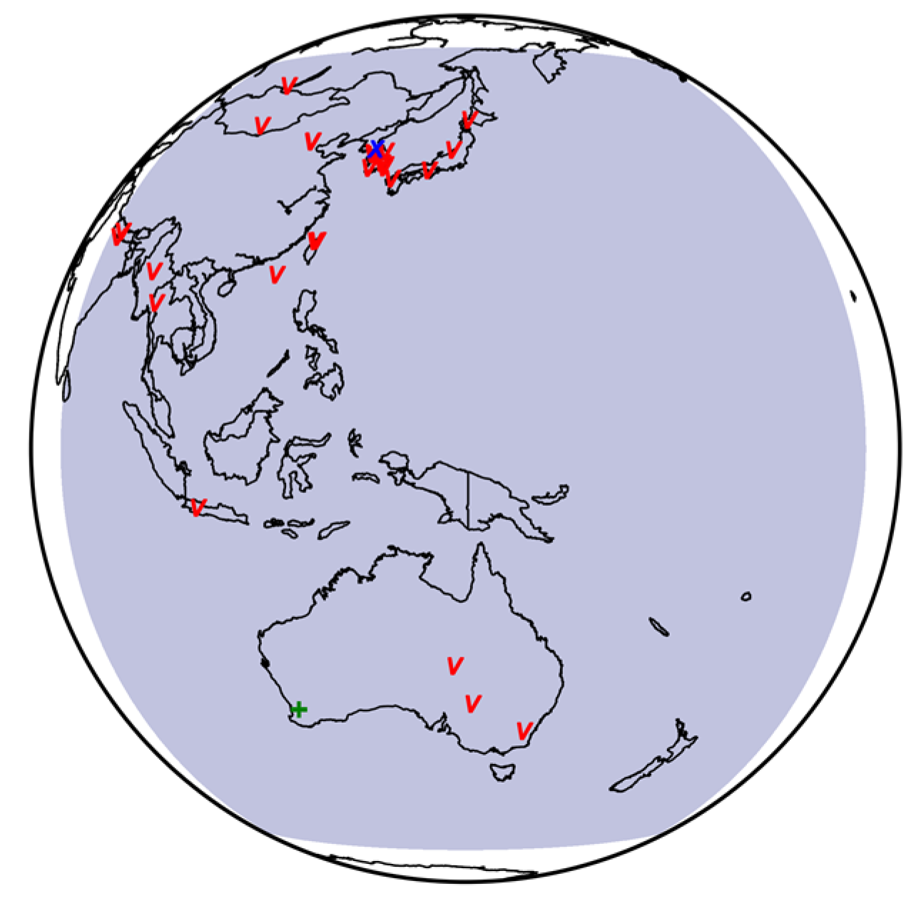
2.2. Ground Measurement Data

2.2.1. AERONET Sites

AERONET is a ground-based observation network that provides atmospheric aerosol properties from the direct and diffuse solar radiation measured using Cimel sun/sky-radiometers [49]. This network has provided globally distributed, long-term, and continuous data for several decades. The retrieval algorithm has developed gradually from Version 1 to the current Version 3, which performs quality control and cloud screening entirely automatically [50]. The AERONET inversion code provides spectral and broadband fluxes at TOA and surface as well as aerosol parameters for three levels of data quality: Level 1.0 (Unscreened), Level 1.5 (Cloud-screened and quality-controlled), and Level 2.0 (quality-assured). The AERONET flux data at the surface were validated by Garcia et al. [51]. We calculated LSA using Level 2.0 surface upward and downward flux data, which are inversion products from the Version 3 algorithm, at the 27 anchor stations (

Table 3. List of ground stations used in this study for validation.

Source	Sites	Latitude (°)	Longitude (°)
AERONET	Bandung	−6.89	107.61
	Beijing-CAMS	39.93	116.31
	Beijing	39.98	116.38
	Birdsville	−25.90	139.35
	Canberra	−35.27	149.11
	Dalanzadgad	43.58	104.42
	Dongsha_Island	20.70	116.73
	EPA-NCU	24.97	121.19
	Fowlers_Gap	−31.09	141.70
	Fukuoka	33.52	130.48
	Gangneung_WNU	37.77	128.87
	Gwangju_GIST	35.23	126.84
	Hankuk_UFS	37.34	127.27
	Hokkaido_University	43.08	141.34
	Irkutsk	51.80	103.09
	KORUS_Kyungpook_NU	35.89	128.60
	KORUS_UNIST_Ulsan	35.58	128.19
	Lumbini	27.49	83.28
	Mandalay_MTU	21.97	96.19
	Niigata	37.85	138.94
	Omkoi	17.80	98.43
	Osaka	34.65	135.59
	Pokhara	28.19	83.98
	Pusan_NU	35.24	129.08
	Seoul_SNU	37.46	126.95
	Taipei_CWB	25.01	121.54
	Yonsei_University	37.56	126.94
OzFlux	Boyagin	−32.51	116.97
KoFlux	CRK	38.20	127.25

). These data are derived using aerosol properties measurements from AERONET sites and are available at AERONET website (https://aeronet.gsfc.nasa.gov/). The inversion products have uncertainties (random error plus biases) that are associated with uncertainty in input data and inversion process such as AOD measurement and absolute sky radiance calibration; thus, various input and post inversion screening criteria were applied for its quality assurance [52]. Only measurements observed at local noon were used for comparison with satellite-based LSA to minimize uncertainty due to differences in observation time between the two observation methods.

2.2.2. OzFlux

OzFlux is an established research network aimed at providing a consistent view of energy, carbon and water exchange to the Australian, New Zealand, and global ecosystem modeling communities [26]. One site (Boyagin) was used in this study due to data availability. This site is located within an area of wandoo woodland (Table 3) and surrounded by broadacre farming practices. The consistent observations such as fluxes, vegetation dynamics, and hydrology were provided from September 2017. The measurements of downward and upward shortwave radiations by a net radiometer (Model CNR4, Kipp & Zonen) at height of 4m has been subject to quality control and post-processing and were used for validation of our results.

2.2.3. KoFlux

The CRK is part of the KoFlux network. This site is located in the Korean Peninsula (Table 3) and is surrounded by rice paddy. The downward and upward shortwave radiations for the entire sky were observed at a height of 9.6 m with net radiometer (Model CNR4, Kipp & Zonen B.V., Delft, The Netherlands) throughout 2017. More detailed information about the CRK site is provided in Hwang et al. [53]. The shortwave radiation observed on this site is averaged every 30 min. For example, the recoded shortwave radiation at 14:00 is the average of the observations from 13:30 to 14:00. To match the reference time between the CRK site observation data and the satellite data, we used the noon observation data. We also used the clearness index presented by Lee et al. [54] to exclude cloud-contaminated shortwave radiation measurements from further analyses.

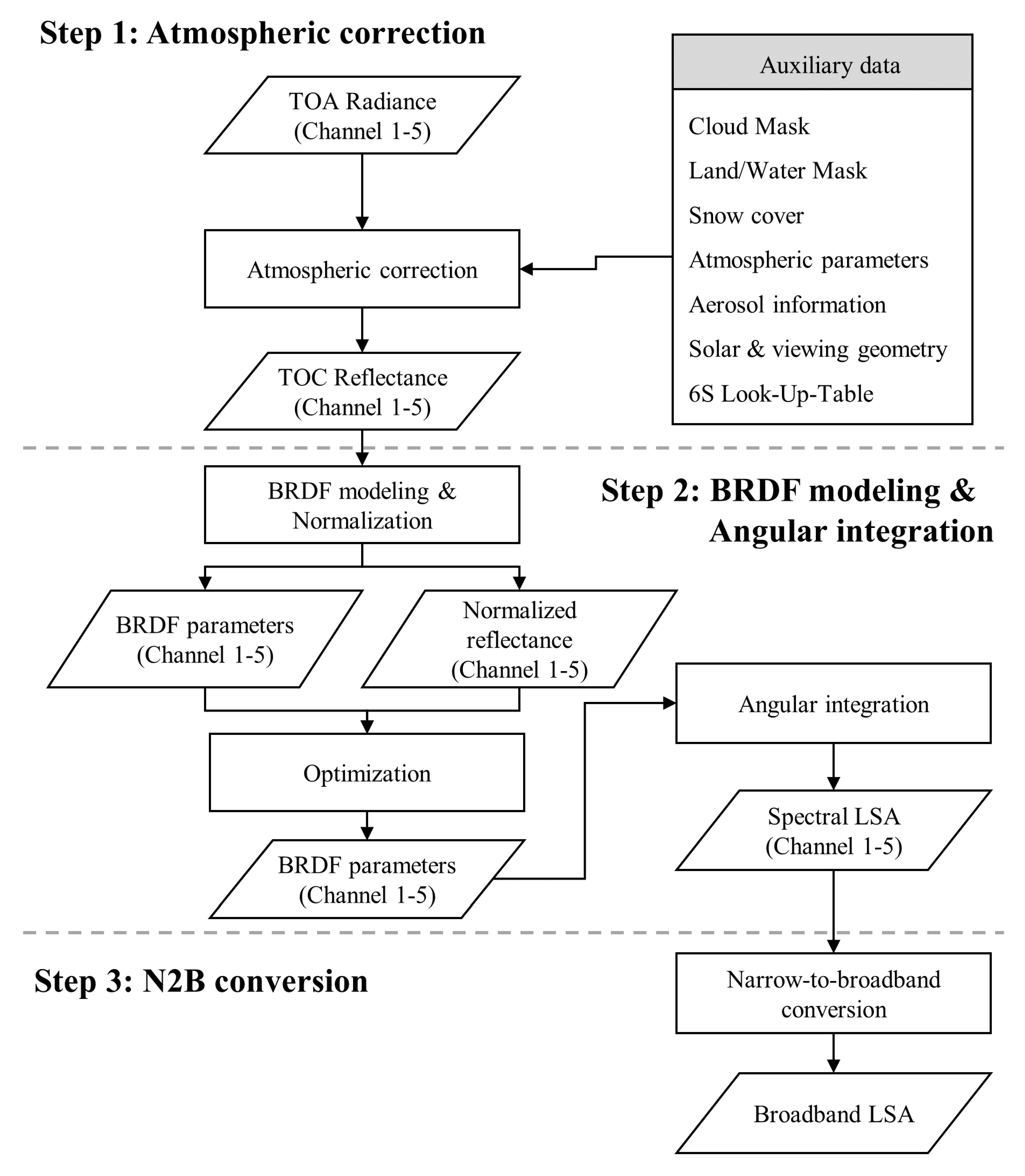
3. Algorithm Development

The overall flow of GK-2A algorithm for LSA retrieval is illustrated in Figure 2. The LSA is estimated through three major steps: atmospheric correction, BRDF modeling, and N2B conversion. These processing steps are intuitive methods of solving the problems in LSA estimation using multi-spectral TOA radiance observed by a satellite sensor [19]. This method is also used for LSA retrieval from the observations of operational satellites, such as MODIS [55] and SEVIRI [30]. The proposed LSA-retrieval algorithm can produce TOC reflectance, surface anisotropy (BRDF parameters), and normalized reflectance for each channel as intermediate products in addition to LSA. These products are applicable in many fields, such as cloud detection [56], aerosol effective height retrieval [57], and monitoring vegetation cover [58]. Details for each processing step are described in the following sections.

3.1. Step 1: Atmospheric Correction

The radiance measured by satellites encounters perturbation as it passes through the atmosphere. Eliminating these atmospheric effects, such as absorption and scattering by molecules and gasses, is an essential process for estimating LSA. We used the 6S vector code to correct for atmospheric effects in TOA radiance measured by AHI. The 6S code is a radiative transfer model that is accurate for simulating atmospheric effect, compared to other methods, such as RT3, MODTRAN, and SHARM [59]. Further details for 6S are provided by Vermote et al. [60]. The 6S model provides three atmospheric correction coefficients: $\mathrm{xa}$ (of inverse of the transmittance), $\mathrm{xb}$ (of the scattering term of the atmosphere), and $\mathrm{xc}$ (of spherical albedo) for given input (atmospheric, aerosol, spectral, and geometric) conditions [61]. To overcome the disadvantage of 6S, which is the long calculation time for application to satellite data, we previously calculated atmospheric correction coefficients for various input conditions as shown in

Table 4. Input parameters of 6S RTM for 6S LUT construction.

Parameter	Input setting
SZA (°)	0, 5, 10, 15, 20, 25, 30, 35, 40, 45, 50, 55, 60, 65, 70, 75, 80
VZA (°)	0, 5, 10, 15, 20, 25, 30, 35, 40, 45, 50, 55, 60, 65, 70, 75, 80
RAA (°)	0, 10, 20, 30, 40, 50, 60, 70, 80, 90, 100, 110, 120, 130, 140, 150, 160, 170, 180
TPW (g cm−2)	0, 1, 2, 3, 4, 5
TCO (atm-cm)	0.25, 0.3, 0.35
AOD	0.01, 0.05, 0.1, 0.15, 0.2, 0.3, 0.4, 0.6, 0.8, 1.0, 1.5, 2.0
Aerosol type	Continental, background desert, maritime

and stored them in LUT form. Atmospheric correction coefficients were calculated with Lambertian surface assumption. This assumption is conflicts with BRDF modeling and can lead the uncertainty in LSA retrieval. However, Lambertian assumption can reduce calculations of 6S and increase the process efficiency of atmospheric correction by reducing the volume of the 6S LUT.

The interval of input parameters that make up the 6S LUT for atmospheric correction can lead to errors in the surface reflectance retrieval, which can cause significant positive or negative errors due to the rapid change in atmospheric effects, especially at high SZA above 70° [40]. Thus, we refine the constructed 6S LUT using the method proposed by Lee et al. [40], which can reduce the error that occurs due to the interval of input parameters, especially high SZA.

We calculated TOC reflectance for each channel using the Equation (1), which is suggested by Vermote et al. [62], for the pixel corresponding to cloud-free, land, and daytime (SZA < 80°)

$${\mathsf{\rho }}_i=\frac{\left(x{a}_i\times L_i-x{b}_i\right)}{1+\left(x{c}_i\times \left(x{a}_i\times L_i-x{b}_i\right)\right)}$$

(1)

where ${\mathsf{\rho }}_i$ and $L_i$ refer to TOC reflectance (unitless) and TOA radiance (${\mathrm{Wm}}^{-2}\mathrm{s}{\mathrm{r}}^{-1}\mu {\mathrm{m}}^{-1}$) at channel $i$, respectively; $x{a}_i$, $x{b}_i$, and $x{c}_i$ refer to the atmospheric correction coefficient for channel $i$ selected in the 6S LUT for the pixel’s observation conditions.

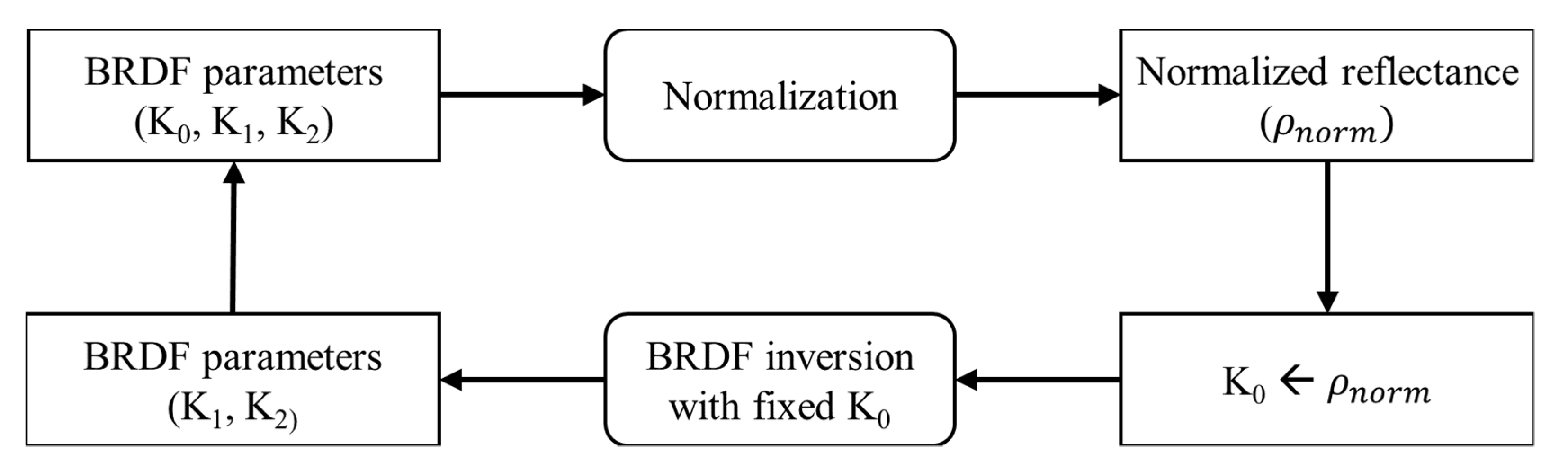
3.2. Step 2: BRDF Model Inversion and Angular Integration

The purpose of this step is the estimation of spectral (narrowband) LSA. The surface albedo means the ratio of downward and upward shortwave radiance for all sun and view geometries. The land surface has anisotropic reflection properties, and it depends on illumination direction, viewing direction, canopy structure such as vegetation density and background characteristic, and wavelengths [63]. Thus, in order to estimate narrowband LSA, the process of estimating the anisotropic reflection characteristics of the surface through the BRDF model and integrating it into the range of the sun/view angle for the hemisphere is necessary [19].

The angular integration was performed to consider surface anisotropy for all angular ranges. The spectral (narrowband) LSA for black-sky and white-sky can be expressed as a linear combination of kernel integration and BRDF parameters (equations (2) and (3)).

$${\alpha }_{bs,\beta }\left({\theta }_s\right)={\displaystyle \sum }_{n=0}^2{K}_{n,\beta }·h_{b,n}\left({\theta }_s\right)$$

(2)

$${\alpha }_{ws,\beta }={\displaystyle \sum }_{n=0}^2{K}_{n,\beta }·h_{w,n}$$

(3)

where

$$h_{b,n}\left({\theta }_s\right)=\frac{1}{\pi }{{\displaystyle \int }}_0^{2\pi }{{\displaystyle \int }}_0^{\pi /2}\left({\theta }_s,{\theta }_v,\varphi \right)sin\left({\theta }_v\right)cos\left({\theta }_v\right)d{\theta }_{v}d\varphi$$

(4)

$$h_{w,n}=2{{\displaystyle \int }}_0^{\pi /2}{h}_{b,n}\left({\theta }_s\right)sin\left({\theta }_s\right)cos\left({\theta }_s\right)d{\theta }_s$$

(5)

In the above equations, ${\alpha }_{bs,\beta }$ and ${\alpha }_{ws,\beta }$ refer to black-sky and white-sky spectral LSA of channel $\beta$. $h_{b,n}$ and $h_{w,n}$ are kernel integration for black-sky and white-sky respectively. ${\theta }_s,{\theta }_v,\mathrm{and}\varnothing$ are SZA, VZA, and RAA, respectively. $f_n$ and $K_{n,\beta }$ are the physical kernels and their weights, respectively, which characterize the anisotropic reflection properties of the land surface.

To describe the land surface anisotropy, we used the kernel-driven BRDF approach. In the semi-empirical model, surface bidirectional reflectance was expressed through a linear combination of three (isotropic, geometric, and volumetric) scattering terms [64]. Each term consists of a kernel that expresses the scattering mechanism of the land surface according to the sun-surface-satellite geometry and the parameter that is the weight of the kernel (Equation (6)).

$${\rho }_{model}=K_0+K_1·f_1\left({\theta }_s,{\theta }_v,\varnothing \right)+K_2·f_2\left({\theta }_s,{\theta }_v,\varnothing \right)$$

(6)

In the above equation, ${\rho }_{model}$ means modeled reflectance by kernel-driven BRDF model at certain angular condition. $K_0$, $K_1$, and $K_2$ refer to BRDF parameters for each scattering term, and $f_1$ and $f_2$ are the physically based kernels for geometric and volumetric scattering. Various kernel-driven BRDF models with different kernels have been proposed, but this study used the Roujean model, which was developed by Roujean et al. [65] and is currently used to obtain LSA from SEVIRI observations [30]. This BRDF model consists of a Ross-Thick (volumetric) kernel and a Roujean (geometric) kernel, and each kernel is calculated as follows:

$$f_1\left({\theta }_s,{\theta }_v,\varphi \right)=\frac{1}{2\pi }\left[\left(\pi -\varphi \right)\cos \varphi +\sin \varphi \right]\tan {\theta }_s\tan {\theta }_v-\frac{1}{\pi }\left(\tan {\theta }_v+\tan {\theta }_s+\sqrt{ta{n}^2{\theta }_v+ta{n}^2{\theta }_s-2\tan {\theta }_s\tan {\theta }_v\cos \varphi }\right)$$

(7)

$$f_2\left({\theta }_s,{\theta }_v,\varphi \right)=\frac{4}{3\pi }·\frac{1}{\cos {\theta }_s+\cos {\theta }_v}\left[\left(\frac{\pi }{2}-\zeta \right)\cos \zeta +\sin \zeta \right]-\frac{1}{3}$$

(8)

where

$$\zeta =\arccos \left[\cos {\theta }_v\cos {\theta }_s+\sin {\theta }_v\sin {\theta }_s\cos \varphi \right]$$

(9)

The empirical BRDF parameters can be calculated through BRDF inversion. For this, linear square regression was applied and the least three observations with various angular conditions in the clear sky are required. Unfortunately, AHI is not a multi-angle sensor; thus, we used time-series data accumulated within a short timeframe to retrieve BRDF parameters. The scheme for BRDF modeling in this algorithm is illustrated in Figure 3. We set the synthesis period to five days, considering the accuracy, processing efficiency, and ratio of the pixel with filling value due to a lack of observations. This period may be shortened, as we use observations measured every 10 min. BRDF modeling is performed with a daily sliding window, and BRDF parameters are retrieved every day. These results are assigned to the final date of the synthesis period.

BRDF modeling has several advantages in analyzing the land surface properties from satellite data, but it occasionally presents significant errors depending on the degree of variability in the angular distribution (e.g., when directional signatures are insufficient) [66,67]. To reduce the errors in BRDF modeling caused by these factors, Roujean [68] proposed using prior knowledge of BRDF parameters. In practice, the current BRDF modeling method used in the MCD43A3 algorithm (version 6) uses a typical BRDF database that is updated with up-to-the-minute retrieval with full inversion for each pixel as prior information [69].

However, this method can constrain the BRDF inversion [70] and is not suitable when the surface condition changes rapidly or the prior knowledge is old. Therefore, in this study, we used normalized reflectance to minimize the errors in BRDF modeling. The normalized reflectance was estimated through the normalization method proposed by Yeom and Kim [71] (Equation 10), which considers the observation characteristics of the geostationary orbit (fixed viewing angles):

$${\rho }_{norm}=\frac{{{\displaystyle \sum }}_{i=1}^n\left({\rho }_{model}\left({\theta }_{s,mean},{\theta }_v,{\varnothing }_{mean}\right)+{\rho }_{measured}\left({\theta }_{s,i},{\theta }_v,{\varnothing }_i\right)-{\rho }_{model}\left({\theta }_{s,i},{\theta }_v,{\varnothing }_i\right)\right)}{n}$$

(10)

where ${\rho }_{norm}$ is the normalized reflectance. ${\rho }_{model}$ and ${\rho }_{measured}$ denote reproduced TOC reflectance using BRDF parameters and measured TOC reflectance, respectively. ${\theta }_{s, mean}$ and ${\varnothing }_{mean}$ are the mean SZA and RAA during the BRDF synthesis period. ${\theta }_{s, i}$ and ${\varnothing }_i$ are the SZA and RAA of the observation number $i$. The $n$ means total number of valid observations for synthesis period. The optimization process scheme is detailed in Figure 4. First, ${\rho }_{norm}$ was calculated using BRDF parameters derived from BRDF inversion using the linear regression method. Then K₀ was modulated with ${\rho }_{norm}$. Lastly, BRDF inversion was performed again for recalculation of K₁ and K₂. In the second BRDF inversion, K₀ was not calculated and was assumed to be a known variable. This process is repeated until the BRDF parameter value stabilizes with little change after that process. The results of the application of the optimization process using BRDF modeling are presented in Section 4.1. The proposed optimization process in this study can performed without any additional information such as prior knowledge.

3.3. Step 3: Broadband LSA Calculation

Limited narrowband wavelengths can be observed by multi-spectral sensors, such as AMI and AHI [72]. This spectral information can be combined via N2B conversion to provide broadband information [73], and this method is applied to several satellite sensors to provide broadband LSA [74]. In this study, broadband LSA for the shortwave domain was calculated using linear combinations of the spectral albedos of AHI and their weights (N2B coefficients), as shown in Equation (11):

$$\mathsf{\Lambda }={\omega }_0+{\omega }_1{\alpha }_1+{\omega }_2{\alpha }_2+{\omega }_3{\alpha }_3+{\omega }_4{\alpha }_4+{\omega }_6{\alpha }_6$$

(11)

where $\mathsf{\Lambda }$ is black-sky (white-sky) broadband LSA, and ${\alpha }_i$ is black-sky (white-sky) narrowband LSA of channel $i$. ${\omega }_i$ is the N2B coefficient of the corresponding spectral LSA. N2B coefficients for snow-free and snow-covered are determined through linear regression analyses using MCD43A3 as reference data. Each dataset contains 18,304 and 803 data entries for snow-free and snow-covered conditions, respectively, with various land types (forest, grasslands, barren, urban, and shrublands). The N2B coefficients for the snow-free and snow-covered conditions of each AHI spectral LSA and the accuracy of linear regression are shown in

Table 5. Results of multiple linear regression. ${\omega }_0$ and ${\omega }_{\mathrm{i}}$ are constant and coefficients for each AHI channel $i$ for converting narrowband albedo to broadband albedo.

	Snow-Free (Black-Sky [White-sky])	Snow-Covered (Black-Ssky [White-sky])
ω0	0.0307 (0.0483)	0.2275 (0.2122)
ω1	−0.2262 (−0.3026)	0.2806 (0.2532)
ω2	0.0481 (0.02956)	0.0373 (0.1101)
ω3	0.5459 (0.6864)	0.0970 0.3319)
ω4	0.1364 (0.1041)	0.2109 (−0.088)
ω5	0.1512 (0.0391)	−0.3183 (−0.1643)
Standard Error	0.0187 (0.0238)	0.0400 (0.0364)
Correlation Coefficient	0.97 (0.92)	0.90 (0.95)

. The results show that all regression results were reasonably accurate with a high R over 0.9 and low standard error under 0.05. In our algorithm, when the TOC reflectance with snow flag was more than half of the total observations during the BRDF modeling synthesis period, snow broadband LSA was calculated using N2B coefficients for the snow-covered conditions.

The quality of broadband LSA data was directly affected by the accuracy of the BRDF modeling [75]. Thus, the quality flag of broadband LSA was designated “good” when the number of observations was higher than seven and the RMSE of BRDF modeling was 0.07 or less; otherwise it was designated “bad”. This classification method is similar to the quality flag classification method used in the MODIS LSA algorithm.

3.4. Quality Assessment

The quality assessment in this study focused on black-sky and white-sky broadband LSA only, although the LSA algorithm we proposed generates several products, including TOC reflectance, BRDF parameters, normalized reflectance, narrowband LSA, and broadband LSA. First, the inter-comparison of AHI and MODIS broadband LSA was carried out to evaluate the overall statistical discrepancy in relation to other satellite-based LSA, spatial consistency, and temporal consistency. Direct comparison with ground measurements from 27 AERONET stations was also performed to evaluate absolute accuracy, and then the AHI results were compared to those of MODIS. The three validation metrics in the form of scalars (RMSE, bias, and R) were used as quantitative indicators of quality. These validation metrics are the most common metrics used to measure accuracy for continuous variables and are expressed as follows:

$$\mathrm{Bias}=\frac{{{\displaystyle \sum }}_{i=1}^n\left(x_i-y_i\right)}{n}$$

(12)

$$\mathrm{RMSE}=\sqrt{\frac{{{\displaystyle \sum }}_{i=1}^n{\left(x_i-y_i\right)}^2}{n}}$$

(13)

$$\mathrm{R}=\frac{{{\displaystyle \sum }}_{i=1}^n\left(x_i-\overline{x}\right)\left(y_i-\overline{y}\right)}{\sqrt{{{\displaystyle \sum }}_{i=1}^n{\left(x_i-\overline{x}\right)}^2}\sqrt{{{\displaystyle \sum }}_{i=1}^n{\left(y_i-\overline{y}\right)}^2}}$$

(14)

In the above equations, $x$ and $y$ denote reference and estimation, respectively; $\overline{x}$ and $\overline{y}$ denote mean of $x$ and $y$, respectively; and $n$ is the number of collocated data entries used for quality assessment.

The validation results of satellite-based LSA compared to ground measurements using the direct comparison method are not always valid due to differences in spatial representation between measurement systems [76]. TC analyses has been suggested as a means of reducing this effect on validation results. This was introduced by Stoffelen et al. [77] and is a method used to estimate the random error variances from three given collocated datasets that have the same geophysical variables [78]. This method makes it possible to estimate the errors of satellite-based products with wide spatial resolution by correcting the ground measurements’ spatial representation errors. For this reason, the TC method has been used to compare various satellite-based geophysical parameters, including LSA, to ground observations [79]. In this analysis, an independent three-measurement system was required, and the RMSE and R of each triplet’s measurement system were calculated [80] as follows:

$$\mathrm{RMSE}=\left[\begin{array}{c}\sqrt{Q_{11}-\frac{Q_{12}{Q}_{13}}{Q_{23}}}\\ \sqrt{Q_{22}-\frac{Q_{12}{Q}_{23}}{Q_{13}}}\\ \sqrt{Q_{33}-\frac{Q_{13}{Q}_{23}}{Q_{12}}}\end{array}\right]$$

(15)

$$R=\left[\begin{array}{c}\sqrt{\frac{Q_{12}{Q}_{13}}{Q_{11}{Q}_{23}}}\\ \sqrt{\frac{Q_{12}{Q}_{23}}{Q_{22}{Q}_{13}}}\\ \sqrt{\frac{Q_{13}{Q}_{23}}{Q_{33}{Q}_{12}}}\end{array}\right]$$

(16)

where $Q_{ij}$ is the covariance between the LSA from the measurement system $\mathrm{i}$ and measurement system $\mathrm{j}$. Each element of the above matrix corresponds to each measurement system of the triplet. In this study, validation metrics calculated using the TC method and validation metrics calculated using direct comparison were compared to determine the effectiveness of the TC method.

In the further analyses, with the exception of time-series analyses, only MODIS and AHI broadband LSA with “good” quality flags were used. The different LSA estimation strategies for snow-covered pixels between AHI and MODIS can also present a difference in broadband LSA [18]. To minimize the error caused by this, when the pixel was snow-covered throughout the entire BRDF modeling synthesis period, it was used to validate snow-covered broadband LSA. However, if the pixel showed no snow cover throughout the entire BRDF modeling synthesis period, it was used for snow-free broadband LSA validation.

4. Results and Discussion

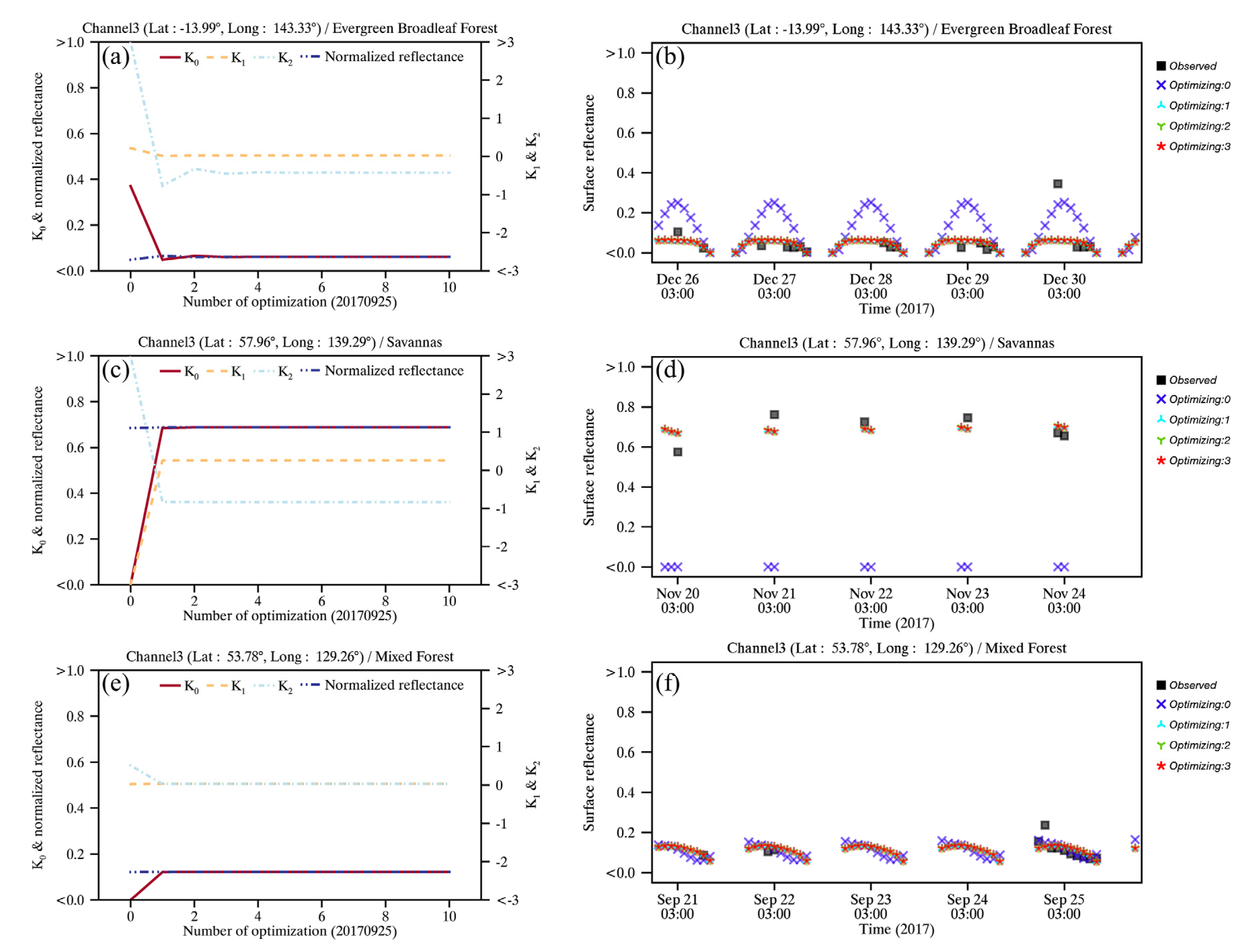
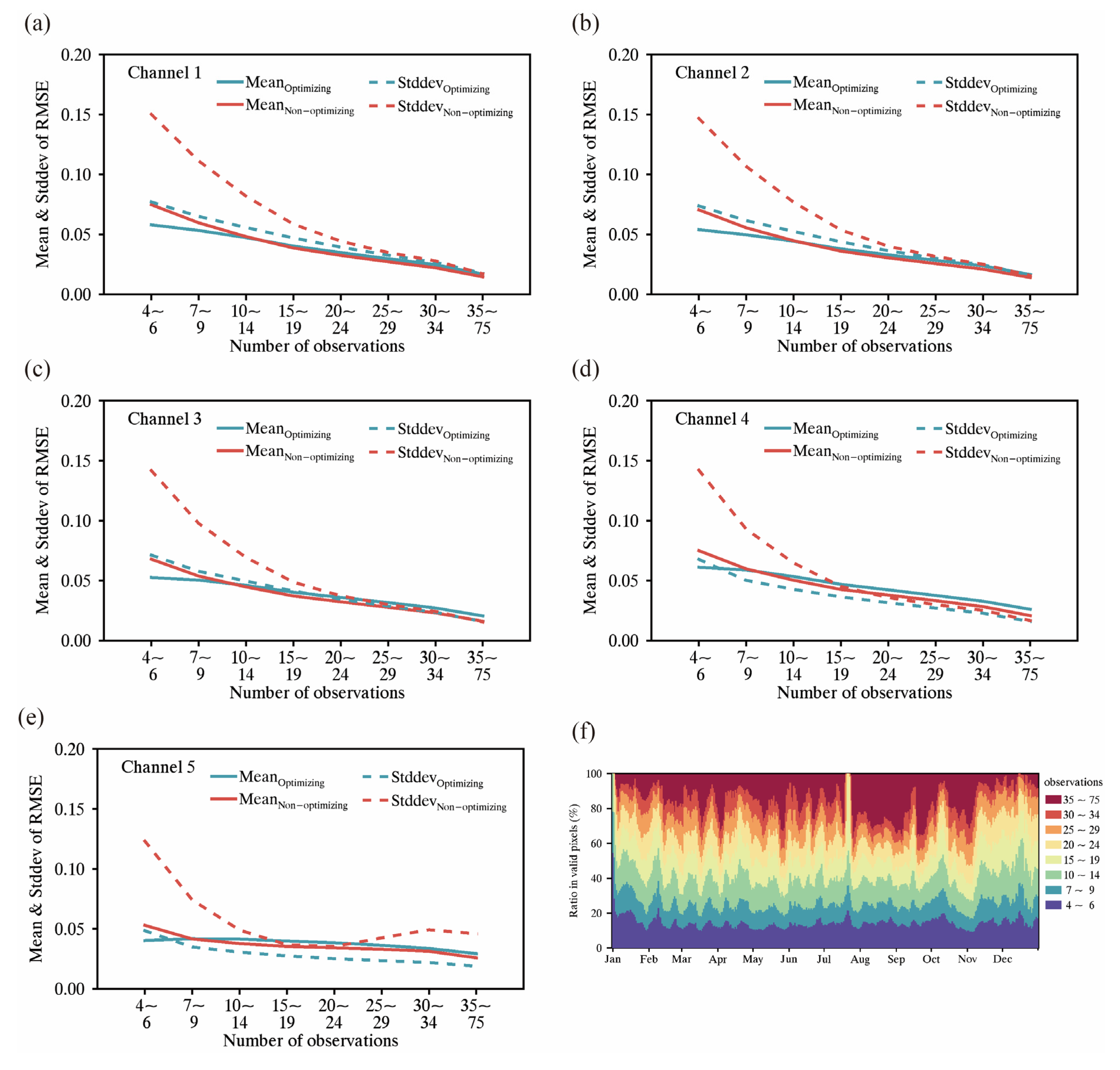
4.1. Optimization of BRDF Modeling

To determine the iteration number for optimization, we analyzed changes in BRDF parameters, ${\rho }_{norm}$, and the reproduced TOC reflectance using BRDF parameters according to the number of optimization processes. These results for three pixels with different cases for channel 3 are shown in Figure 5. The same results were obtained for the other channels and have been omitted for brevity.

The first row (Figure 5a,b) shows when the RMSE of BRDF modeling was reduced from 0.1208 to 0.0704 after optimization. As Figure 5a shows, before the optimization process, the value of K₀ was abnormally high (almost 0.4), although this pixel’s land type is an evergreen broadleaf forest located in Northern Australia (tropical north). For this reason, the value of K₂ was also abnormally high at over 3. Therefore, the TOC reflectance reproduced using the BRDF parameter without an optimization process shows a higher value than the typical reflectance for that land type, and the variation is also considerable. This error was caused by a cloud classification error that occurred on December 30 at 01:00 UTC (Figure 5b). After the optimization process, K₀ and K₂ decreased. The reproduced TOC reflectance showed better agreement with the TOC reflectance observed in cloudless conditions, and the variability was also reduced. This result showed that optimization processing can help to improve the quality of BRDF inversion when some observations are contaminated by clouds. The second row (Figure 5c,d) shows the results for snow-covered pixels located at high latitudes in the northern hemisphere. As shown in Figure 5d, all observations of the pixel were made at a similar local time. Therefore, the angle information sampled from this pixel was limited to a fixed view and a narrow solar geometry range (77.93–79.84°). In such cases, an error can occur when BRDF inversion is due to insufficient angular information [54]. In practice, as shown in Figure 5c,d, all three BRDF parameters calculated prior to optimization showed abnormal values, and the reproduced TOC reflectance was less than 0, indicating a value outside the valid range. The BRDF inversion result improved after the optimization process and showed similar improvements to the previous case. The last row (Figure 5e,f) shows the case when BRDF inversion RMSE was slightly increased after optimization from 0.0285 to 0.0369. Even before the optimization was performed, the TOC reflectance reproduced from the BRDF parameters appeared to simulate the surface anisotropy reflectance of the observed TOC reflectance. Even before the optimization was performed, the reproduced TOC reflectance closely simulates the surface anisotropy characteristics of the observed TOC reflectance (Figure 5f). Nevertheless, K₀ has a negative value outside the valid range, as shown in Figure 5e. After optimization, K₀ showed a positive value, and the reproduced TOC reflectance closely simulated the observation TOC reflectance prior to optimization.

These results show that the optimization process using ${\rho }_{norm}$ improves errors that occur for various reasons, such as cloud contamination and limited angular range in BRDF inversion. This can be useful when no a prior information is available. The changes in BRDF parameters and normalized reflectivity according to the number of repetitions of optimization change up to three times, but little change occurs subsequently. Moreover, the reproduced TOC reflectance does not show a significant difference depending on the number of optimization iterations. Therefore, considering the processing efficiency and accuracy, it was deemed appropriate to perform the optimization process three times.

Figure 6a shows the mean and standard deviations of the RMSE of the reproduced TOC reflectance by BRDF modeling based on the number of observations for each channel before and after the optimization process over one year. Mean and standard deviation of RMSE tend to decrease as the number of observations increases in all channels except channel 5. The mean RMSE of BRDF modeling was lowered in all channels after the optimization process when the number of observations was lower than nine. However, when the number of observations was 15 or more, RMSE increased after the optimization process. However, the increase in RMSE is small, up to 0.0053 in channel 4. This is also a reasonable result when RMSE increases despite the improvement of BRDF inversion, as shown in Figure 5e,f. The standard deviation of RMSE was improved in all cases after the optimization process, however. In particular, the fewer observations, the more remarkable the improvement, and when fewer than six observations were made, the standard deviation decreased by about half. In Figure 6f, pixels with 24 observations or fewer account for more than 50% of the total valid pixels every day. Therefore, the optimization process using ${\rho }_{norm}$ improved the accuracy of BRDF inversion without a prior knowledge accumulation for most pixels.

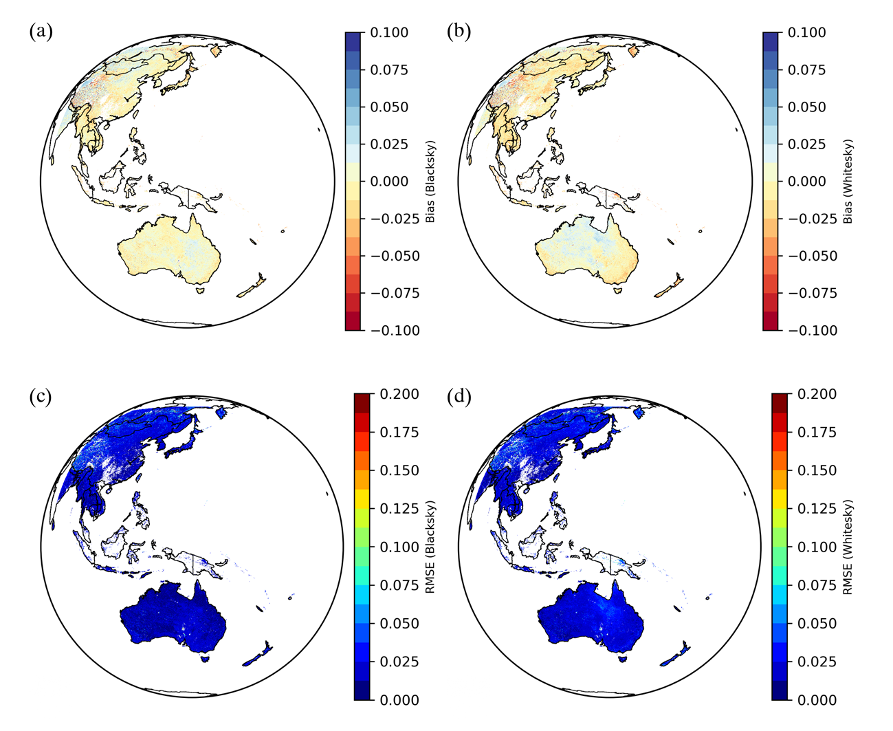
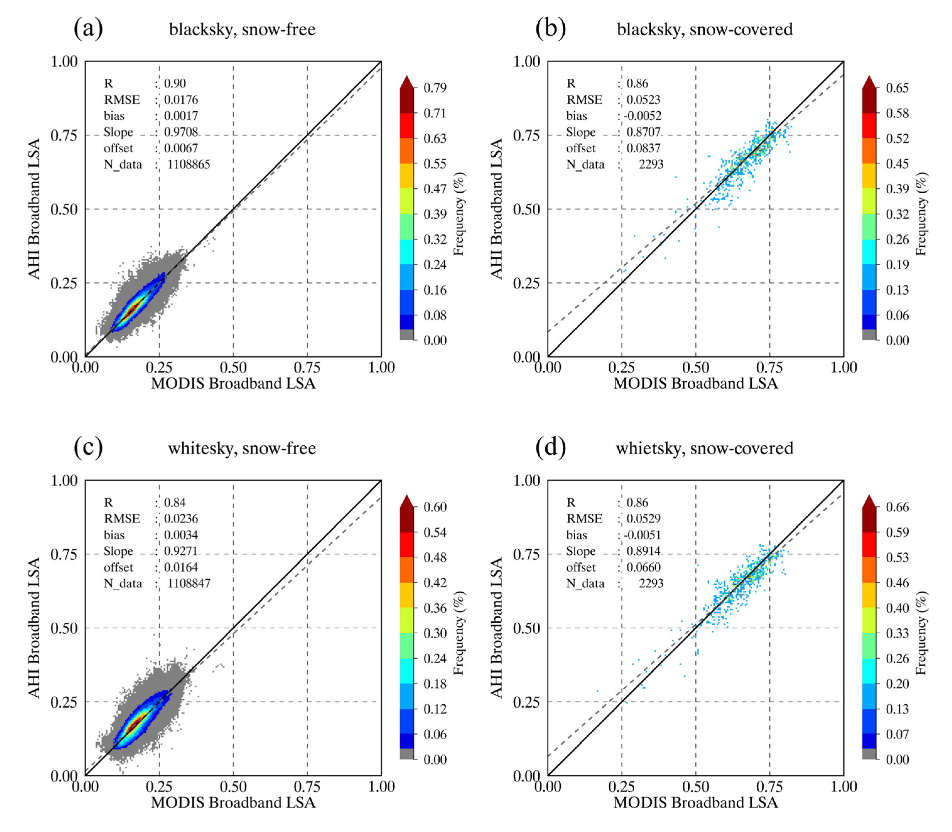
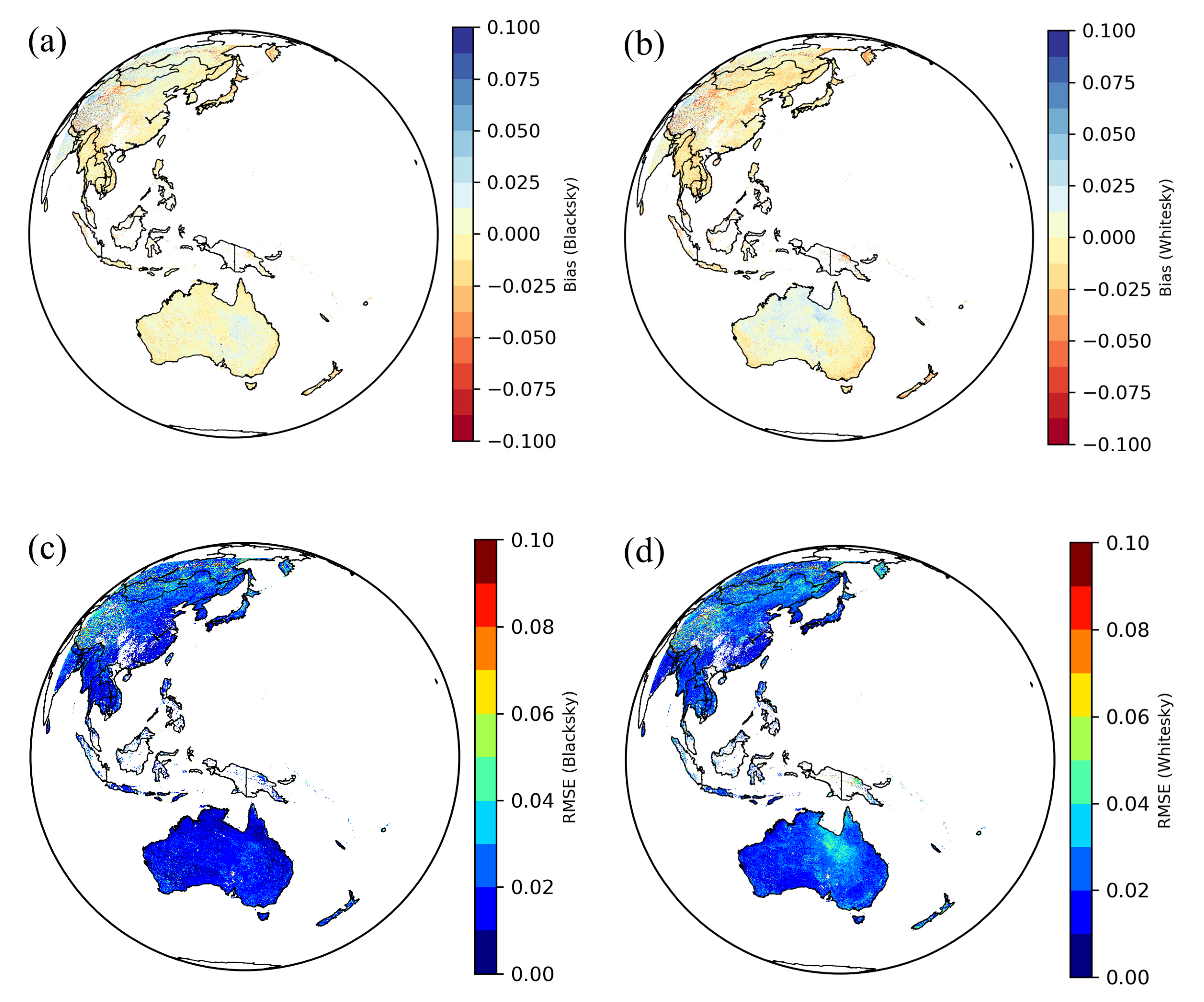
4.2. Inter-Comparison with MODIS LSA Product

The broadband LSA derived from AHI was compared to that from MODIS. Figure 7a,c show the difference in broadband LSA estimated from AHI and MODIS for black-sky and white-sky under snow-free conditions. Most pixels were located close to the 1:1 line. Although the AHI broadband LSA values are generally higher than those of MODIS, with the positive bias of 0.0017 for black-sky and 0.0034 for white-sky, they are negligible and generally show good agreement overall. The validation metrics of black-sky (RMSE of 0.0176, bias of 0.0017, and R of 0.90) showed slightly improved results compared to those of white-sky (RMSE of 0.0236, bias of 0.0034, and R of 0.84). Moreover, each point of white-sky is more widely distributed from the diagonal than those of black-sky. Figure 7b,d show comparison results of broadband LSA in snow-covered pixels. Most of pixels are located close to the 1:1 line and show good agreement overall. The higher RMSE that is 0.0523 for black-sky and 0.0529 for white-sky in snow-free conditions is reasonable when the high broadband LSA of the snow-covered pixels is considered [3,81]. Unlike the comparison results for snow-free conditions, AHI broadband LSA was lower than that of MODIS with a negative bias of -0.0052 for black-sky and −0.0051 for white-sky. The accuracies of snow-covered pixels for black-sky and white-sky were similar with close validation metrics (RMSE, bias, and R). Consequently, these results indicate that black-sky and white-sky AHI broadband LSA agree well overall with MODIS broadband LSA, which was well validated in both snow-free and snow-covered conditions, although some differences are evident between these sensors, such as cloud detection, snow cover detection, the synthesis period of BRDF modeling, spectral information, and angular sampling.

Figure 8 shows the statistical difference for one year between AHI and MODIS broadband LSA in geographic distribution. In the vicinity of the equator and in southern China, there were no high-quality MODIS pixels for a year, so it was marked in white to indicate the fill value. As shown in Figure 8a,b, the salient characteristic is that most pixels have a low bias within ±0.025 for both black-sky and white-sky. Relatively large positive or negative bias was shown in the regions of western China. The region is characterized by frequent cloud cover [82]. Thus, these features in bias may be related to the difference between satellite-based cloud retrievals from the two sensors. The regions with high VZAs, such as eastern India, also show a relatively high positive bias. This may also be related to cloud masking of AHI because geostationary satellites perform relatively weakly in cloud masking for regions with large VZA [83]. In the higher latitudes of the northern hemisphere, such as southern Russia and the Kamchatka Peninsula, a slight negative bias is present due to snow cover in the winter season. Generally, the white-sky bias was larger than that of black-sky. In practice, white-sky bias showed a slightly positive bias, unlike black-sky in Australia. This result is in accordance with the results presented in Figure 7. The geographic distribution of RMSE for black-sky and white-sky (Figure 8c,d) shows similar results to those related to bias. Of all valid black-sky and white-sky pixels, 96.41% and 95.73%, respectively, show accuracy within the 0.02–0.05 range that is required as absolute retrieval accuracy by climate models across a range of spatial and temporal scales [84] compared to MODIS. Therefore, AHI broadband LSA has good spatial consistency with MODIS broadband LSA.

The temporal comparisons of the black-sky broadband LSA with the MODIS data for five land types (barren [41.09°N, 99.70°E], croplands [38.53°N, 125.57°E], grasslands [47.04°N, 117.19°E], mixed forest [48.20°N, 129.00°E], and open shrublands [22.88°S, 115.58°E]) are presented in Figure 9. The results for white-sky were similar to those for black-sky; thus, they have been omitted for brevity. For the barren land (Figure 9a), the LSA shows a stable value with around 0.22 throughout the year. However, the LSA of AHI shows little temporal variability compared to that of MODIS. The misclassification of clouds may occur in the barren region due to its spectral signature, which is similar to cloud cover [85]. This indicates that the error in TOC reflectance due to misclassification of clouds affects the accuracy of the LSA. The broadband LSA of AHI and MODIS showed a difference within ±0.05, indicating a good overall agreement. In the case of pixels corresponding to croplands (Figure 9b), seasonal variation in the LSA was well expressed in both AHI and MODIS. The broadband LSA tends to decrease over time until summer, which corresponds to the vegetation growing season, and in the later period, the broadband LSA increases in association with the aging of vegetation. During some summer periods (DOY 170–199 and 215–231) when the land surface was frequently covered by clouds, broadband LSA was not estimated from MODIS whereas AHI broadband LSA was retrieved. This demonstrates the advantages of AHI’s high temporal resolution. This advantage can be maximized by taking observations every 10 min. As Figure 9c illustrates, broadband LSA has a large range from about 0.2 during the snow-free period to around 0.8 during the snow-covered period. The broadband LSA from both AHI and MODIS have slightly different values due to the different broadband LSA calculation strategies for snow-covered pixels but show a similar change during the snow melting period in the spring and snowfall periods in winter. However, at the end of the snow melting season (DOY 89–97), MODIS broadband LSA was high when covered with snow, although it was not classified as a “snow” flag in the MCD43A2. This is thought to be due to a cloud and snow cover detection error in the snow melting season and MODIS’ relatively long BRDF synthesis period (16 days). AHI broadband LSA closely followed the changes in the ratio of snow covered observation to valid observation during the BRDF synthesis period. Even in the pixel corresponding to the mixed forest (Figure 9d), the change in AHI albedo in winter (DOY 1–85 and 315–365) corresponds well with the ratio of snow-covered observations. The MODIS broadband LSA was not retrieved during the same period. In the other periods, the AHI broadband LSA shows a slightly larger variation than MODIS in summer. The majority of retrieved LSAs show a difference of 0.05 or less. Figure 9e shows the time-series of LSA from AHI and MODIS for open shrublands. This case is hardly affected by clouds and snow. Thus, AHI broadband LSA closely follows that of MODIS all year round with a difference within ±0.03.

The above result shows that AHI broadband LSA was temporarily consistent with that of MODIS. Furthermore, AHI broadband LSA expresses seasonal variation well in addition to rapid changes due to snowfall and snowmelt, while the temporal variation in AHI was slightly higher than that of MODIS. The AHI can provide broadband LSA with improved temporal completeness thanks to its high temporal resolution in areas with frequent cloud or where snow and cloud are difficult to distinguish. When all observations taken every 10 min are used to estimate the LSA, it is expected that the temporal completeness will improve further and that the quality of the data produced will also improve.

The broadband LSA varies somewhat according to land type and time. The AHI broadband LSA was compared to that of MODIS for some land types and months (Figure 10). The forest type indicates that all five land types (evergreen broadleaf, evergreen needle-leaf, deciduous broadleaf, deciduous needle-leaf, and mixed forest) are combined into one. Both black-sky and white-sky exhibit low RMSE (from 0.0157 to 0.0270 in black-sky and from 0.0216 to 0.0302 in white-sky) and bias (from −0.0042 to 0.0066 in black-sky and from −0.0117 to 0.0014 in white-sky) for all land types (Figure 10a,b). The variation in bias in different land types was slightly greater in white-sky than black-sky, but it was nonetheless negligible. In Figure 10c,d, the RMSE between AHI and MODIS broadband LSA was almost stable in black-sky (from 0.0160 to 0.0203), while the monthly RMSE in white-sky showed a slightly larger variation according to time (from 0.0180 to 0.0287). The reason for this error tendency may be that the error generated in the atmospheric correction and BRDF modeling step was amplified by the integration of the BRDF kernel for the SZA to calculate the white-sky spectral LSA [32]. Nevertheless, both black-sky and white-sky show reasonable differences with an RMSE smaller than 0.05.

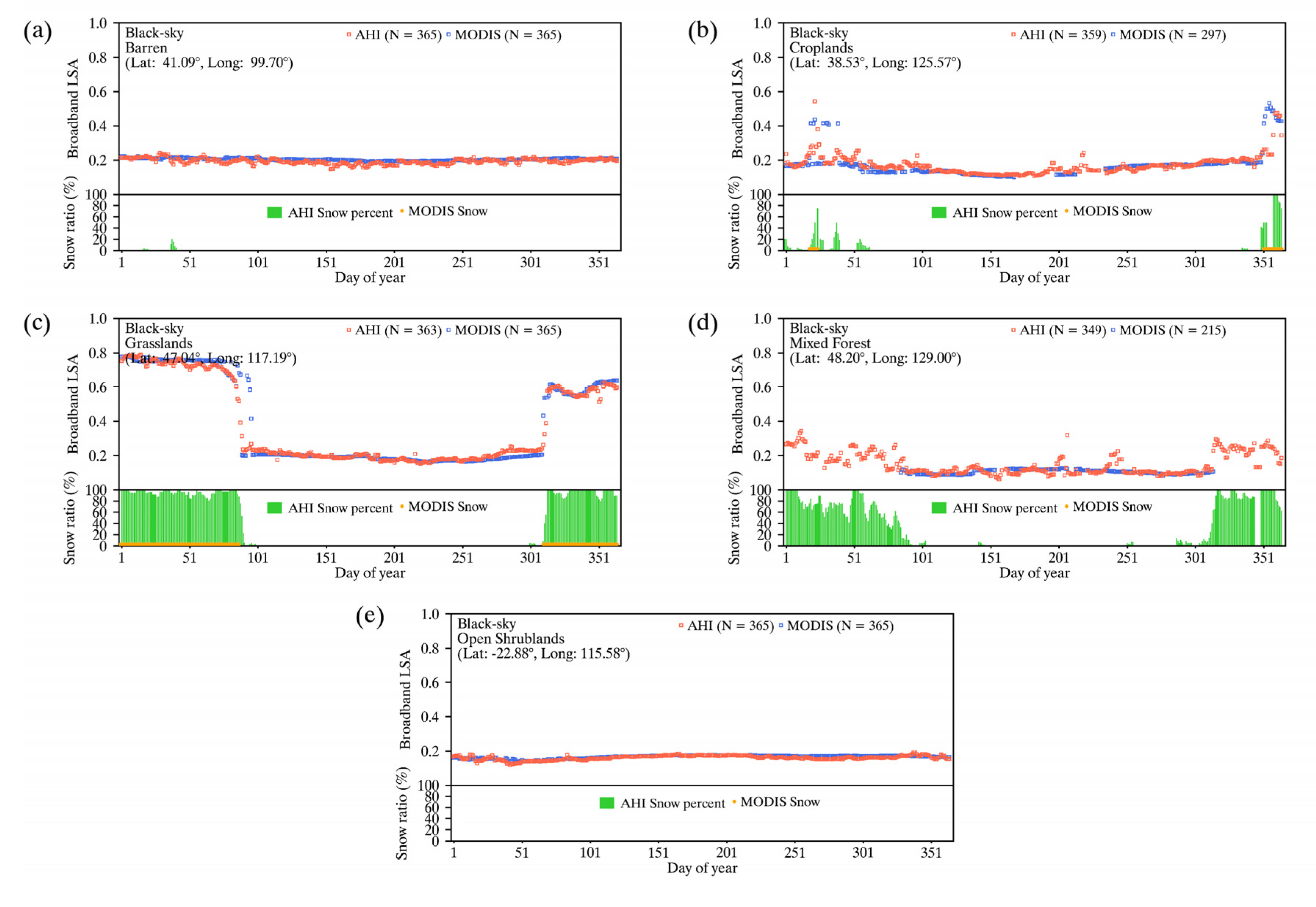
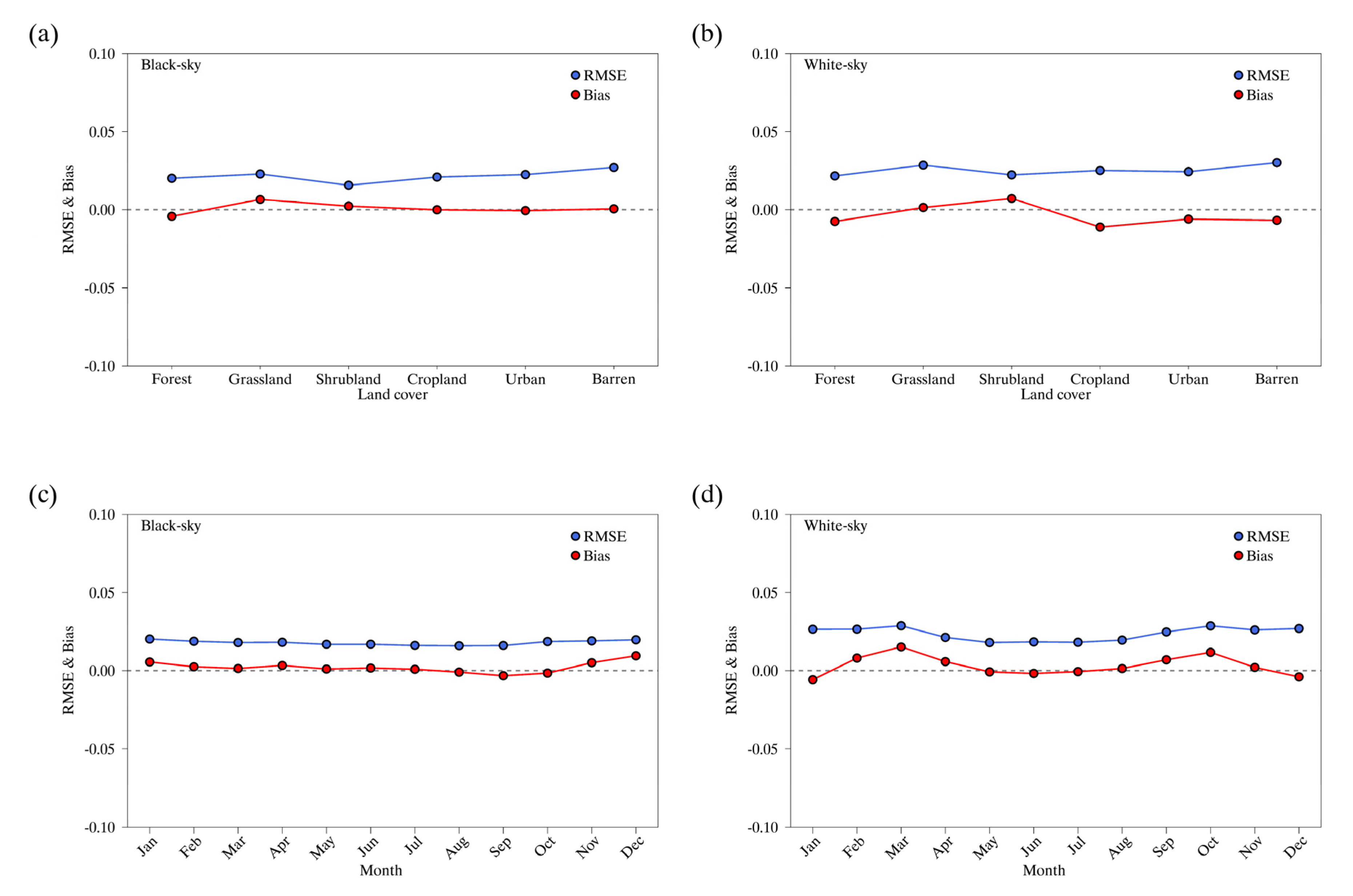
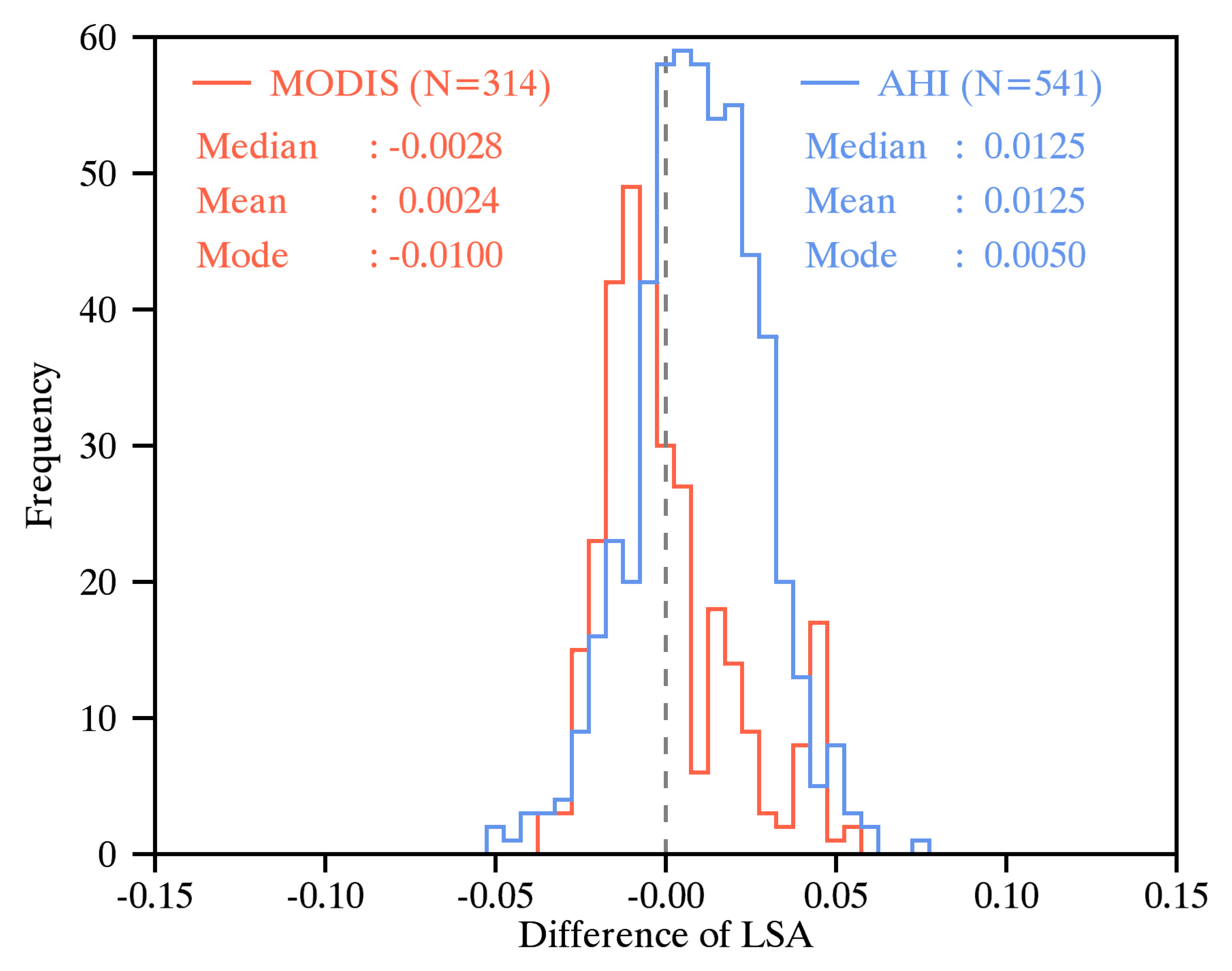
4.3. Accuracy Evaluation Using Ground Measurements

The results of validation using all available spatial-temporal matchup data between satellite-based LSA and ground measurements from AERONET sites and Boyagin site are shown in

Table 6. Results of accuracy assessment retrieved from the direct comparison of AHI and MODIS broadband LSA versus ground measurements from 27 AERONET sites and Boyagin site for snow-free conditions over the 2017 year. The term N indicates the number of observations used in accuracy assessment.

Sites	AHI			MODIS
	RMSE	Bias	N	RMSE	Bias	N
Bandung	0.0108	−0.0072	8	-	-	0
Beijing-CAMS	0.0432	0.0419	22	0.0051	0.0006	3
Beijing	0.0386	0.0360	19	0.0090	−0.0072	7
Birdsville	0.0237	0.0232	26	0.0235	0.0227	26
Canberra	0.0089	−0.0004	45	0.0048	0.0043	41
Dalanzadgad	0.0196	0.0106	25	0.0208	0.0169	21
Dongsha_Island	0.0507	0.0507	1	-	-	0
EPA-NCU	0.0129	0.0071	9	0.0021	−0.0021	1
Fowlers_Gap	0.0176	0.0159	20	0.0067	-0.0058	20
Fukuoka	0.0127	0.0123	7	-	-	0
Gangneung_WNU	0.0189	−0.0012	30	0.0196	−0.0190	23
Gwangju_GIST	0.0142	0.0116	5	-	-	0
Hankuk_UFS	0.0198	0.0013	27	0.0094	−0.0029	22
Hokkaido_University	0.0215	−0.0114	10	-	-	0
Irkutsk	-	-	0	0.0561	0.0561	1
KORUS_Kyungpook_NU	0.0153	0.0153	2	-	-	0
KORUS_UNIST_Ulsan	0.0083	0.0082	5	0.0127	0.0125	5
Lumbini	0.0301	0.0285	23	0.0236	−0.0236	2
Mandalay_MTU	0.0220	0.0114	34	0.0100	−0.0089	20
Niigata	0.0153	0.0040	11	-	-	0
Omkoi	0.0111	−0.0087	19	0.0047	−0.0030	21
Osaka	0.0156	0.0060	39	-	-	0
Pokhara	0.0212	0.0162	67	0.0146	−0.0130	61
Pusan_NU	-	-	0	0.0045	−0.0045	1
Seoul_SNU	0.0164	0.0113	27	0.0091	−0.0079	8
Taipei_CWB	0.0095	0.0066	3	-	-	0
Yonsei_University	0.0336	0.0308	30	0.0204	0.0203	4
Boyagin	0.0170	0.0133	27	0.0469	0.0468	27
All sites	0.0223	0.0125	541	0.0195	0.0024	314

. In general, AHI shows the tendency to overestimate with a bias of 0.0125. This leads to an RMSE that is somewhat slightly worse in AHI (0.0223) than that in MODIS (0.0195). At some sites, such as “Beijing-CAMS”, “Beijing”, “Dongsha_Island”, “Lumbini”, and “Yonsei_University”, bias over 0.025 is indicated and shows a relatively higher magnitude of overestimation than other sites. These sites have over three times more retrievals in the case of AHI than in the case of MODIS in common. Therefore, this trend of overestimation may be caused by differences in the cloud mask between the two sensors. Nonetheless, AHI broadband LSA outlines good overall consistency with ground measurements, which is comparable to the validation results of [26]. Moreover, in the case of the Boyagin site, MODIS shows a greater positive bias than AHI. In most sites (except three: “Irkutsk,” “Omkoi,” and “Pusan_NU”), the number of AHI samples was higher than that of MODIS, and the total number of AHI samples was 541, far larger than 317. This indicates that AHI has better completeness and can provide a larger number of valid pixels in the Asia–Oceania region, thanks to its high temporal resolution.

The histogram of the difference between the ground measurements and the satellite-based LSA from AHI and MODIS (Figure 11) has almost normal distribution for AHI and right-skewed distribution for MODIS. Although the AHI tends to overestimate compared to the ground measurement with a positive mean (0.0125) and median (0.0125) of difference, 97.4% of collocation data show an absolute difference within 0.05. The largest difference was 0.079 at the Beijing site, which may be attributable to an error in TOC reflectance by large aerosol loading [26]. In addition, AHI has a slightly better mode (i.e., the value where the histogram reaches its peak) than MODIS.

As mentioned, when comparing a satellite-based LSA with a kilometer-scale spatial resolution to ground observations, some errors may occur due to differences in spatial representation between the data. We conducted an evaluation using the TC method to address the issue related to spatial representation, and then compared the results with the results achieved using a direct comparison method (

Table 7. Comparison of validation results between the direct comparison and triple collocation methods; 284 triplets were used in this analysis.

	Direct Comparison		Triple Collocation
	RMSE	R	RMSE	R
AHI	0.0178	0.9542	0.0126	0.9648
MODIS	0.0196	0.9221	0.0178	0.9323

). The results of the direct comparison presented in Table 7 differ from the results shown in Table 6 and Figure 11 because these analyses were used only for comparison when all three data sets (ground measurement, AHI, and MODIS) were valid. For both AHI and MODIS, the TC method yielded slightly better RMSE and R than direct comparison. This indicates that the TC method can help to compare between two data sets with different spatial representations. As mentioned by Wu et al. [80], because the TC technique does not completely correct for the difference in spatial representation between the ground measurement and the satellite data, no significant improvement in RMSE or R² was observed for either AHI or MODIS. Another reason for this result is that the TC technique involves several assumptions, which are not always met [79].

Figure 12 shows the time-series of satellite-derived broadband LSA and ground measurements for the CRK site. The AHI and MODIS broadband LSA reasonably captured the seasonal variation in ground measurements. In addition, the RMSE of AHI and MODIS broadband LSA was 0.0309 and 0.0316, respectively, which is less than the required accuracy for climate models. Both AHI and MODIS broadband LSA showed negative bias of −0.0193 and −0.0229, respectively. This error may be due to following two reason: (1) the difference in the reference time between the ground measurement from the CRK site (average from local noon to the next 30 min) and the satellite-based broadband LSA (instantaneous at local noon), (2) difference in spatial representation between two measurement systems. The AHI broadband LSA value was greater than that of MODIS throughout 2017 due to its high temporal resolution. This advantage is particularly pronounced during the summer months when it is hot and humid and the rain can persist for long periods. During the DOY 170–236, which is usually a long rainy season, AHI can provide broadband LSA while MODIS has no LSA retrieval capabilities. This indicates that AHI is more useful for the retrieval of broadband LSA when clouds are frequently present.

5. Conclusions

In this study, we developed an LSA-retrieval algorithm with the operational purpose of retrieving LSA in clear-sky conditions from GK-2A/AMI, South Korea’s next-generation geostationary meteorological satellite. Due to GK-2A/AMI’s short operation period, the proposed algorithm was developed using Himawari-8/AHI, which has similar channel specifications to GK-2A/AMI in the shortwave domain. The LSA was retrieved through three major steps: atmospheric correction, BRDF modeling, and N2B conversion. To perform each processing step, we adopted the 6S RTM, the Roujean BRDF model, and the multiple linear regression method and optimized the geostationary satellite observation system. In particular, the iterative optimization process used in BRDF modeling would work well to improve the accuracy of BRDF inversions, and the improvement was evident when the number of observations taken during the BRDF composite period was below nine. The multiple linear regression results for deriving N2B conversion coefficients were also reliable for both snow-free and snow-covered conditions with a low standard error of less than 0.05 and a high R of over 0.9.

The black-sky and white-sky broadband LSA retrieved from AHI was compared to MODIS LSA product to evaluate its overall quality over the period of a year. In general, black-sky (white-sky) broadband LSA from AHI shows good overall consistency with that of MODIS in snow-free conditions with RMSE of 0.0176 (0.0236), bias of 0.0017 (0.0034), and R of 0.90 (0.84). Although the RMSE was slightly higher than the required accuracy of broadband LSA in the climate model (0.02–0.05) for snow-covered conditions, it was reasonable when its high value was considered. In addition, AHI broadband LSA shows good spatial and temporal consistency with MODIS broadband LSA. In most AHI full-disk domains, except for some pixels that were frequently covered by cloud, AHI broadband LSA shows a difference lower than 0.05 for both black-sky and white-sky, and AHI broadband LSA expressed diurnal variation in broadband LSA well over one year for five land types. The results of validation with ground measurements from 27 AERONET sites show that our results showed slightly higher RMSE (0.0223) than the MODIS RMSE (0.0195), and a weak positive bias is indicated. Although AERONET downward and upward fluxes used in this study were well validated [51], these are not direct measurement and most sites are located in heterogeneous areas. Thus, validation with direct measurements from other flux networks is needed for a more reliable quality assessment. AHI provides more valid LSA data than MODIS due to its high temporal resolution and despite of its relatively short BRDF synthesis period. Moreover, the mode value of the difference was close to 0. This advantage will be increased when AHI data observed every 10 min is used. When the TC technique was used, the accuracy was slightly improved, but no significant improvement was observed. This is similar to the results presented by Wu et al. [80]. AHI broadband LSA reasonably captured diurnal variation in ground measurements from the CRK site and showed improved temporal completeness in particular when clouds were frequently observed.

Our retrieval algorithm performs well to provide high-quality LSA with high spatial and temporal completeness from geostationary satellite observations in the Asia–Oceania region. We believe that this algorithm will be applied to GK-2A, the Republic of Korea’s next-generation meteorological satellite. LSA data with high spatial and temporal resolution from the proposed algorithm can be utilized in various fields, such as validation of model results [11], simulation of weather and climate [86], and radiation budget studies [87]. Nevertheless, further research is necessary to improve and ensure the quality of LSA derived from the proposed algorithm. Further study is required to assess the stability of the LSA using long-term data and to validate LSA for more extensive spatial and temporal coverage, including snow-covered conditions to meet the validation stage 3 presented by the Committee on Earth Observation Satellites Land Product Validation subgroup.

References

1. Pokrovsky, O.; Roujean, J.L. Land surface albedo retrieval via kernel-based BRDF modeling: II. An optimal design scheme for the angular sampling. Remote Sens. Environ. 2003, 84, 120–142. [Google Scholar] [CrossRef]
2. Raschke, E.; Vonder Haar, T.H.; Bandeen, W.R.; Pasternak, M. The annual radiation balance of the earth-atmosphere system during 1969–70 from Nimbus 3 measurements. J. Atmos. Sci. 1973, 30, 341–364. [Google Scholar] [CrossRef] [Green Version]
3. Pohl, C.; Istomina, L.; Tietsche, S.; Jäkel, E.; Stapf, J.; Spreen, G.; Heygster, G. Broadband albedo of Arctic sea ice from MERIS optical data. Cryosphere 2020, 14, 165–182. [Google Scholar] [CrossRef] [Green Version]
4. Wang, Z.; Schaaf, C.B.; Sun, Q.; Kim, J.; Erb, A.M.; Gao, F.; Román, M.O.; Yang, Y.; Petroy, S.; Taylorm, J.R.; et al. Monitoring land surface albedo and vegetation dynamics using high spatial and temporal resolution synthetic time series from Landsat and the MODIS BRDF/NBAR/albedo product. Int. J. Appl. Earth Obs. Geoinf. 2017, 59, 104–117. [Google Scholar] [CrossRef]
5. Zhao, X.; Liang, S.; Liu, S.; Yuan, W.; Xiao, Z.; Liu, Q.; Cheng, J.; Zhang, X.; Tang, H.; Zhang, X.; et al. The Global Land Surface Satellite (GLASS) remote sensing data processing system and products. Remote Sens. 2013, 5, 2436–2450. [Google Scholar] [CrossRef] [Green Version]
6. Andrews, T.; Betts, R.A.; Booth, B.B.; Jones, C.D.; Jones, G.S. Effective radiative forcing from historical land use change. Clim. Dyn. 2017, 48, 3489–3505. [Google Scholar] [CrossRef]
7. Li, Q.; Ma, M.; Wu, X.; Yang, H. Snow cover and vegetation-induced decrease in global albedo from 2002 to 2016. J. Geophys. Res. Atmos. 2018, 123, 124–138. [Google Scholar] [CrossRef] [Green Version]
8. Boussetta, S.; Balsamo, G.; Dutra, E.; Beljaars, A.; Albergel, C. Assimilation of surface albedo and vegetation states from satellite observations and their impact on numerical weather prediction. Remote Sens. Environ. 2015, 163, 111–126. [Google Scholar] [CrossRef] [Green Version]
9. He, T.; Liang, S.; Wang, D.; Chen, X.; Song, D.X.; Jiang, B. Land surface albedo estimation from Chinese HJ satellite data based on the direct estimation approach. Remote Sens. 2015, 7, 5495–5510. [Google Scholar] [CrossRef] [Green Version]
10. Brest, C.L.; Goward, S.N. Deriving surface albedo measurements from narrow band satellite data. Int. J. Remote Sens. 1987, 8, 351–367. [Google Scholar] [CrossRef]
11. Csiszar, I.; Gutman, G. Mapping global land surface albedo from NOAA AVHRR. J. Geophys. Res. Atmos. 1999, 104, 6215–6228. [Google Scholar] [CrossRef]
12. Manninen, T.; Aalto, T.; Markkanen, T.; Peltoniemi, M.; Böttcher, K.; Metsämäki, S.; Anttila, K.; Pirinen, P.; Leppänen, A.; Arslan, A.N. Monitoring changes in forestry and seasonal snow using surface albedo during 1982–2016 as an indicator. Biogeosciences 2019, 16, 223–240. [Google Scholar] [CrossRef] [Green Version]
13. Zhou, C.; Zhang, T.; Zheng, L. The characteristics of surface albedo change trends over the Antarctic sea ice region during recent decades. Remote Sens. 2019, 11, 821. [Google Scholar] [CrossRef] [Green Version]
14. Zhou, M.; Chen, G.; Dong, Z.; Xie, B.; Gu, S.; Shi, P. Estimation of surface albedo from meteorological observations across China. Agric. For. Meteorol. 2020, 281, 107848. [Google Scholar] [CrossRef]
15. Qu, Y.; Liang, S.; Liu, Q.; He, T.; Liu, S.; Li, X. Mapping surface broadband albedo from satellite observations: A review of literatures on algorithms and products. Remote Sens. 2015, 7, 990–1020. [Google Scholar] [CrossRef] [Green Version]
16. Riihelä, A.; Manninen, T.; Key, J.; Sun, Q.; Sütterlin, M.; Lattanzio, A.; Schaaf, C. A Multisensor Approach to Global Retrievals of Land Surface Albedo. Remote Sens. 2018, 10, 848. [Google Scholar] [CrossRef] [Green Version]
17. Wang, Z.; Schaaf, C.B.; Sun, Q.; Shuai, Y.; Román, M.O. Capturing Rapid Land Surface Dynamics with Collection V006 MODIS BRDF/NBAR/Albedo (MCD43) Products. Remote Sens. Environ. 2018, 207, 50–64. [Google Scholar] [CrossRef]
18. Roujean, J.L.; Leon-Tavares, J.; Smets, B.; Claes, P.; De Coca, F.C.; Sanchez-Zapero, J. Surface albedo and toc-r 300 m products from PROBA-V instrument in the framework of Copernicus Global Land Service. Remote Sens. Environ. 2018, 215, 57–73. [Google Scholar] [CrossRef]
19. He, T.; Wang, D.; Qu, Y. Land surface albedo. In Comprehensive Remote Sensing; Elsevier: Amsterdam, The Netherlands, 2018; Volume 5, pp. 140–162. [Google Scholar] [CrossRef]
20. Liang, S.; Wang, D.; Zhou, Y.; Yu, Y.; Peng, J. VIIRS NDE Surface Albedo Algorithm Theoretical Basis Document. 2018. Available online: https://pdfs.semanticscholar.org/d812/b1ef99b9ea84b1df0e9caaecebd30dead8ab.pdf (accessed on 12 April 2020).
21. Pinty, B.; Roveda, F.; Verstraete, M.; Gobron, N.; Govaerts, Y.; Martonchik, J.; Diner, D.; Kahn, R. Surface albedo retrieval from METEOSAT: Part 1. Theory. J. Geophys. Res. 2000, 105, 18099–18112. [Google Scholar] [CrossRef]
22. Lattanzio, A.; Schulz, J.; Matthews, J.; Okuyama, A.; Theodore, B.; Bates, J.J.; Kosaka, Y.; Schüller, L. Land surface albedo from geostationary satellites: A multiagency collaboration within SCOPE-CM. Bull. Am. Meteorol. 2013, 94, 205–214. [Google Scholar] [CrossRef]
23. Geiger, B.; Carrer, D.; Franchisteguy, L.; Roujean, J.L.; Meurey, C. Land surface albedo derived on a daily basis from Meteosat second generation observations. IEEE Trans. Geosci. Remote Sens. 2008, 46, 3841–3856. [Google Scholar] [CrossRef]
24. Proud, S.R.; Rasmussen, M.O.; Fensholt, R.; Sandholt, I.; Shisanya, C.; Mutero, W.; Mbow, C.; Anyamba, A. Improving the smac atmospheric correction code by analysis of meteosat second generation ndvi and surface reflectance data. Remote Sens. Environ. 2010, 114, 1687–1698. [Google Scholar] [CrossRef]
25. He, T.; Liang, S.L.; Wang, D.; Wu, H.; Yu, Y.; Wang, J. Estimation of surface albedo and directional reflectance from Moderate Resolution Imaging Spectroradiometer (MODIS) observations. Remote Sens. Environ. 2012, 119, 286–300. [Google Scholar] [CrossRef] [Green Version]
26. He, T.; Zhang, Y.; Liang, S.; Yu, Y.; Wang, D. Developing Land Surface Directional Reflectance and Albedo Products from Geostationary GOES-R and Himawari Data: Theoretical Basis, Operational Implementation, and Validation. Remote Sens. 2019, 11, 2655. [Google Scholar] [CrossRef] [Green Version]
27. Schaaf, C.B.; Gao, F.; Strahler, A.H.; Lucht, W.; Li, X.; Tsang, T.; Strugnell, N.C.; Zhang, X.; Jin, Y.; Muller, J.-P.; et al. First operational BRDF, albedo nadir reflectance products from MODIS. Remote Sens. Environ. 2002, 83, 135–148. [Google Scholar] [CrossRef] [Green Version]
28. He, T.; Liang, S.; Wang, D. Direct Estimation of Land Surface Albedo from Simultaneous MISR Data. IEEE Trans. Geosci. Remote Sens. 2017, 55, 2605–2617. [Google Scholar] [CrossRef]
29. Carrer, D.; Smets, B.; Ceamanos, X.; Roujean, J.L. Copernicus Global Land Operations “Vegetation and Energy”. 2017. Available online: https://land.copernicus.eu/global/sites/cgls.vito.be/files/products/CGLOPS1_ATBD_SA1km-V1_I2.11.pdf (accessed on 1 June 2020).
30. Carrer, D.; Moparthy, S.; Lellouch, G.; Ceamanos, X.; Pinault, F.; Freitas, S.C.; Trigo, I.F. Land surface albedo derived on a ten daily basis from Meteosat Second Generation Observations: The NRT and climate data record collections from the EUMETSAT LSA SAF. Remote Sens. 2018, 10, 1262. [Google Scholar] [CrossRef] [Green Version]
31. Asner, G.P.; Wessman, C.A.; Schimel, D.S.; Archer, S. Variability in leaf and litter optical properties: Implications for BRDF model inversions using AVHRR, MODIS, and MISR. Remote Sens. Environ. 1998, 63, 243–257. [Google Scholar] [CrossRef]
32. Lee, C.S.; Han, K.S.; Yeom, J.M.; Lee, K.S.; Seo, M.; Hong, J.; Hong, J.W.; Lee, K.; Shin, J.; Shin, I.C.; et al. Surface albedo from the geostationary Communication, Ocean and Meteorological Satellite (COMS)/Meteorological Imager (MI) observation system. GISci. Remote Sens. 2018, 55, 38–62. [Google Scholar] [CrossRef]
33. Liang, S. A direct algorithm for estimating land surface broadband albedos from MODIS imagery. IEEE Trans. Geosci. Remote Sens. 2003, 41, 136–145. [Google Scholar] [CrossRef]
34. Bessho, K.; Date, K.; Hayashi, M.; Ikeda, A.; Imai, T.; Inoue, H.; Kumagai, Y.; Miyakawa, H.; Murata, H.; Ohno, T.; et al. An introduction to Himawari-8/9—Japan’s new-generation geostationary meteorological satellites. J. Meteorol. Soc. Jpn. 2016, 94, 151–183. [Google Scholar] [CrossRef] [Green Version]
35. Yang, J.; Zhang, Z.; Wei, C.; Lu, F.; Guo, Q. Introducing the new generation of Chinese geostationary weather satellites, Fengyun-4. Bull. Am. Meteorol. 2017, 98, 1637–1658. [Google Scholar] [CrossRef]
36. Goodman, S.J. GOES-R Series Introduction. In The GOES-R Series; Elsevier: Amsterdam, The Netherlands, 2020; pp. 1–3. [Google Scholar] [CrossRef]
37. Descheemaecker, M.; Plu, M.; Marécal, V.; Claeyman, M.; Olivier, F.; Aoun, Y.; Blanc, P.; Wald, L.; Guth, J.; Sič, B.; et al. Monitoring aerosols over Europe: An assessment of the potential benefit of assimilating the VIS04 measurements from the future MTG/FCI geostationary imager. Atmos. Meas. Tech. 2019, 12, 1251–1275. [Google Scholar] [CrossRef] [Green Version]
38. Oh, S.M.; Borde, R.; Carranza, M.; Shin, I.C. Development and Intercomparison Study of an Atmospheric Motion Vector Retrieval Algorithm for GEO-KOMPSAT-2A. Remote Sens. 2019, 11, 2054. [Google Scholar] [CrossRef] [Green Version]
39. National Meteorological Satellite Center Home Page. Available online: https://nmsc.kma.go.kr/enhome/html/base/cmm/selectPage.do?page=satellite.gk2a.intro (accessed on 1 April 2020).
40. Lee, K.S.; Lee, C.S.; Seo, M.; Choi, S.; Seong, N.H.; Jin, D.; Yeom, J.M.; Han, K.S. Improvements of 6S Look-Up-Table Based Surface Reflectance Employing Minimum Curvature Surface Method. Asia Pac. J. Atmos. Sci. 2020, 3, 1–14. [Google Scholar] [CrossRef] [Green Version]
41. Seong, N.H.; Jung, D.; Kim, J.; Han, K.S. Evaluation of NDVI Estimation Considering Atmospheric and BRDF Correction through Himawari-8/AHI. Asia-Pac. J. Atmos. Sci. 2020, 5, 1–10. [Google Scholar] [CrossRef] [Green Version]
42. He, M.; Wang, D.; Ding, W.; Wan, Y.; Chen, Y.; Zhang, Y. A Validation of Fengyun4A Temperature and Humidity Profile Products by Radiosonde Observations. Remote Sens. 2019, 11, 2039. [Google Scholar] [CrossRef] [Green Version]
43. Wei, J.; Li, Z.; Sun, L.; Peng, Y.; Zhang, Z.; Li, Z.; Su, T.; Feng, L.; Cai, Z.; Wu, H. Evaluation and uncertainty estimate of next-generation geostationary meteorological Himawari-8/AHI aerosol products. Sci. Total Environ. 2019, 692, 879–891. [Google Scholar] [CrossRef]
44. Zhang, W.; Xu, H.; Zhang, L. Assessment of Himawari-8 AHI Aerosol Optical Depth Over Land. Remote Sens. 2019, 11, 1108. [Google Scholar] [CrossRef] [Green Version]
45. Lee, K.S.; Jin, D.; Yeom, J.M.; Seo, M.; Choi, S.; Kim, J.J.; Han, K.S. New Approach for Snow Cover Detection through Spectral Pattern Recognition with MODIS Data. J. Sens. 2017, 2017, 4820905. [Google Scholar] [CrossRef]
46. National Meteorological Satellite Center Home Page. Available online: https://nmsc.kma.go.kr/homepage/html/base/cmm/selectPage.do?page=static.edu.atbdGk2a (accessed on 1 April 2020).
47. Lee, C.S.; Yeom, J.M.; Lee, H.L.; Kim, J.J.; Han, K.S. Sensitivity analysis of 6S-based look-up table for surface reflectance retrieval. Asia-Pac. J. Atmos. Sci. 2015, 51, 91–101. [Google Scholar] [CrossRef]
48. Wang, K.; Liu, J.; Zhou, X.; Sparrow, M.; Ma, M.; Sun, Z.; Jiang, W. Validation of the MODIS global land surface albedo product using ground measurements in a semidesert region on the Tibetan Plateau. J. Geophys. Res. Atmos. 2004, 109, D05107. [Google Scholar] [CrossRef]
49. Holben, B.N.; Eck, T.F.; Slutsker, I.A.; Tanre, D.; Buis, J.P.; Setzer, A.; Vermote, E.; Reagan, J.A.; Kaufman, Y.J.; Nakajima, T.; et al. AERONET—A federated instrument network and data archive for aerosol characterization. Remote Sens. Environ. 1998, 66, 1–16. [Google Scholar] [CrossRef]
50. Sicard, M. Validation of AERONET-Estimated Upward Broadband Solar Fluxes at the Top-Of-The-Atmosphere with CERES Measurements. Remote Sens. 2019, 11, 2168. [Google Scholar] [CrossRef] [Green Version]
51. García, O.E.; Díaz, A.M.; Expósito, F.J.; Díaz, J.P.; Dubovik, O.; Dubuisson, P.; Rojer, J.C.; Eck, T.F.; Sinyuk, A.; Derimian, Y.; et al. Validation of AERONET estimates of atmospheric solar fluxes and aerosol radiative forcing by ground-based broadband measurements. J. Geophys. Res. Atmos. 2008, 113. [Google Scholar] [CrossRef]
52. Holben, B.N.; Eck, T.F.; Slutsker, I.; Smirnov, A.; Sinyuk, A.; Schafer, J.; Giles, D.; Dubovik, O. Aeronet’s Version 2.0 quality assurance criteria. Proc. SPIE 2006, 6408, 64080Q. [Google Scholar]
53. Hwang, Y.; Ryu, Y.; Huang, Y.; Kim, J.; Iwata, H.; Kang, M. Comprehensive assessments of carbon dynamics in an intermittently-irrigated rice paddy. Agric. For. Meteorol. 2020, 285, 107933. [Google Scholar] [CrossRef]
54. Lee, S.; Ryu, Y.; Jiang, C. Urban heat mitigation by roof surface materials during the East Asian summer monsoon. Environ. Res. Lett. 2015, 10, 124012. [Google Scholar] [CrossRef]
55. Strahler, A.; Muller, J.; Lucht, W.; Schaaf, C.; Tsang, T.; Gao, F.; Li, X.; Lewis, P.; Barnsley, M. MODIS BRDF/Albedo Product: Algorithm Theoretical Basis Document Version 5.0. Available online: http://www.researchgate.net/publication/234144971_MODIS_BRDF_Albedo_Product_ATBD_V_5.0 (accessed on 5 March 2020).
56. Yeom, J.M.; Roujean, J.L.; Han, K.S.; Lee, K.S.; Kim, H.W. Thin cloud detection over land using background surface reflectance based on the BRDF model applied to Geostationary Ocean Color Imager (GOCI) satellite data sets. Remote Sens. Environ. 2020, 239, 111610. [Google Scholar] [CrossRef]
57. Choi, W.; Lee, H.; Kim, J.; Ryu, J.Y.; Park, S.S.; Park, J.; Kang, H. Effects of spatiotemporal O4 column densities and temperature-dependent O4 absorption cross-section on an aerosol effective height retrieval algorithm using the O4 air mass factor from the ozone monitoring instrument. Remote Sens. Environ. 2019, 229, 223–233. [Google Scholar] [CrossRef]
58. Zhang, X.; Friedl, M.A.; Schaaf, C.B.; Strahler, A.H.; Hodges, J.C.; Gao, F.; Reed, B.C.; Huete, A. Monitoring vegetation phenology using MODIS. Remote Sens. Environ. 2003, 84, 471–475. [Google Scholar] [CrossRef]
59. Kotchenova, S.Y.; Vermote, E.F.; Levy, R.; Lyapustin, A. Radiative transfer codes for atmospheric correction and aerosol retrieval: Intercomparison study. Appl. Opt. 2008, 47, 2215–2226. [Google Scholar] [CrossRef] [PubMed] [Green Version]
60. Vermote, E.F.; Tanré, D.; Deuze, J.L.; Herman, M.; Morcette, J.J. Second simulation of the satellite signal in the solar spectrum, 6S: An overview. IEEE Trans. Geosci. Remote. Sens. 1997, 35, 675–686. [Google Scholar] [CrossRef] [Green Version]
61. Darge, Y.M.; Hailu, B.T.; Muluneh, A.A.; Kidane, T. Detection of geothermal anomalies using Landsat 8 TIRS data in Tulu Moye geothermal prospect, Main Ethiopian Rift. Int. J. Appl. Earth Obs. Geoinf. 2019, 74, 16–26. [Google Scholar] [CrossRef]
62. Vermote, E.; Tanré, D.; Deuzé, J.L.; Herman, M.; Morcrette, J.J.; Kotchenova, S.Y. Second Simulation of A Satellite Signal in the Solar Spectrum-Vector (6SV); 6S User Guide Version 3. Available online: http://6s.ltdri.org/files/tutorial/6S_Manual_Part_1.pdf (accessed on 11 July 2020).
63. Calleja, J.F.; Recondo, C.; Peón, J.; Fernández, S.; De la Cruz, F.; González-Piqueras, J. A New Method for the Estimation of Broadband Apparent Albedo Using Hyperspectral Airborne Hemispherical Directional Reflectance Factor Values. Remote Sens. 2016, 8, 183. [Google Scholar] [CrossRef] [Green Version]
64. Kim, S.I.; Ahn, D.S.; Han, K.S.; Yeom, J.M. Improved Vegetation Profiles with GOCI Imagery Using Optimized BRDF Composite. J. Sens. 2016, 2016, 7. [Google Scholar] [CrossRef]
65. Roujean, J.L.; Leroy, M.; Deschamps, P.Y. A bidirectional reflectance model of the Earth’s surface for the correction of remote sensing data. J. Geophys. Res. Atmos. 1992, 97, 20455–20468. [Google Scholar] [CrossRef]
66. Duchemin, B.; Maisongrande, P. Normalisation of directional effects in 10-day global syntheses derived from VEGETATION/SPOT: I. Investigation of concepts based on simulation. Remote Sens. Environ. 2002, 81, 90–100. [Google Scholar] [CrossRef]
67. Han, K.S.; Champeaux, J.L.; Roujean, J.L. A land cover classification product over France at 1 km resolution using SPOT4/VEGETATION data. Remote Sens. Environ. 2004, 92, 52–66. [Google Scholar] [CrossRef]
68. Roujean, J.-L. Inversion of Lumped Parameters Using BRDF Kernels. In Comprehensive Remote Sensing; Elsevier: Amsterdam, The Netherlands, 2018; Volume 3, pp. 23–34. [Google Scholar] [CrossRef]
69. University of Massachusetts Boston Home Page. Available online: https://www.umb.edu/spectralmass/terra_aqua_modis/modis_brdf_albedo_product_mcd43 (accessed on 7 March 2020).
70. Wang, Y.; Li, X.; Nashed, Z.; Zhao, F.; Yang, H.; Guan, Y.; Zhang, H. Regularized kernel-based brdf model inversion method for ill-posed land surface parameter retrieval. Remote Sens. Environ. 2007, 111, 36–50. [Google Scholar] [CrossRef]
71. Yeom, J.M.; Kim, H.O. Feasibility of using Geostationary Ocean Colour Imager (GOCI) data for land applications after atmospheric correction and bidirectional reflectance distribution function modelling. Int. J. Remote Sens. 2013, 34, 7329–7339. [Google Scholar] [CrossRef]
72. Peng, S.; Wen, J.; Xiao, Q.; You, D.; Dou, B.; Liu, Q.; Tang, Y. Multi-Staged NDVI Dependent Snow-Free Land-Surface Shortwave Albedo Narrowband-to-Broadband (NTB) Coefficients and Their Sensitivity Analysis. Remote Sens. 2017, 9, 93. [Google Scholar] [CrossRef] [Green Version]
73. Schaaf, C.B.; Martonchik, J.; Pinty, B.; Govaerts, Y.; Gao, F.; Lattanzio, A.; Liu, J.; Strahler, A.; Taberner, M. Retrieval of surface albedo from satellite sensors. In Advances in Land Remote Sensing: System, Modeling, Inversion and Application; Liang, S., Ed.; Springer: Houten, The Netherlands, 2008; pp. 219–243. [Google Scholar] [CrossRef]
74. Liang, S. Narrowband to broadband conversions of land surface albedo I: Algorithms. Remote Sens. Environ. 2001, 76, 213–238. [Google Scholar] [CrossRef]
75. Liu, Y.; Wang, Z.; Sun, Q.; Erb, A.M.; Li, Z.; Schaaf, C.B.; Zhang, X.; Román, M.O.; Scott, R.L.; Zhang, Q.; et al. Evaluation of the VIIRS BRDF, Albedo and NBAR products suite and an assessment of continuity with the long term MODIS record. Remote Sens. Environ. 2017, 201, 256–274. [Google Scholar] [CrossRef]
76. Gruber, A.; Dorigo, W.A.; Zwieback, S.; Xaver, A.; Wagner, W. Characterizing Coarse-Scale Representativeness of in situ Soil Moisture Measurements from the International Soil Moisture Network. Vadose Zone J. 2013, 12, 1–16. [Google Scholar] [CrossRef] [Green Version]
77. Stoffelen, A. Toward the true near-surface wind speed: Error modeling and calibration using triple collocation. J. Geophys. Res. Oceans 1998, 103, 7755–7766. [Google Scholar] [CrossRef]
78. McColl, K.A.; Vogelzang, J.; Konings, A.G.; Entekhabi, D.; Piles, M.; Stoffelen, A. Extended triple collocation: Estimating errors and correlation coefficients with respect to an unknown target. Geophys. Res. Lett. 2014, 41, 6229–6236. [Google Scholar] [CrossRef] [Green Version]
79. Gruber, A.; Su, C.H.; Zwieback, S.; Crow, W.; Dorigo, W.; Wagner, W. Recent advances in (soil moisture) triple collocation analysis. Int. J. Appl. Earth Obs. Geoinf. 2016, 45, 200–211. [Google Scholar] [CrossRef]
80. Wu, X.; Xiao, Q.; Wen, J.; You, D. Direct Comparison and Triple Collocation: Which Is More Reliable in the Validation of Coarse-Scale Satellite Surface Albedo Products. J. Geophys. Res. Atmos. 2019, 124, 5198–5213. [Google Scholar] [CrossRef]
81. Molotch, N.P.; Bales, R.C. Comparison of ground-based and airborne snow surface albedo parameterizations in an alpine watershed: Impact on snowpack mass balance. Water Resour. Res. 2006, 42, W05410. [Google Scholar] [CrossRef] [Green Version]
82. Wu, F.; Fu, C. Assessment of GEWEX/SRB version 3.0 monthly global radiation dataset over China. Meteorol. Atmos. Phys. 2011, 112, 155. [Google Scholar] [CrossRef]
83. Kraatz, S.; Khanbilvardi, R.; Romanov, P. A comparison of MODIS/VIIRS cloud masks over ice-bearing river: On achieving consistent cloud masking and improved river ice mapping. Remote Sens. 2017, 9, 229. [Google Scholar] [CrossRef] [Green Version]
84. Govaerts, Y.; Lattanzio, A. Estimation of surface albedo increase during the eighties Sahel drought from Meteosat observations. Glob. Planet. Chang. 2008, 64, 139–145. [Google Scholar] [CrossRef]
85. Jeppesen, J.H.; Jacobsen, R.H.; Inceoglu, F.; Toftegaard, T.S. A cloud detection algorithm for satellite imagery based on deep learning. Remote Sens. Environ. 2019, 229, 247–259. [Google Scholar] [CrossRef]
86. Lim, Y.J.; Byun, K.Y.; Lee, T.Y.; Kwon, H.; Hong, J.; Kim, J. A land data assimilation system using the MODIS-derived land data and its application to numerical weather prediction in East Asia. Asia-Pac. J. Atmos. Sci. 2012, 48, 83–95. [Google Scholar] [CrossRef]
87. Seo, M.; Kim, H.-C.; Huh, M.; Yeom, J.-M.; Lee, C.S.; Lee, K.-S.; Choi, S.; Han, K.-S. Long-Term Variability of Surface Albedo and Its Correlation with Climatic Variables over Antarctica. Remote Sens. 2016, 8, 981. [Google Scholar] [CrossRef] [Green Version]
Figure 1. The map of the AHI full-disk area. The area used in this study is shaded light blue. The red symbol “v”, green symbol “+”, and blue symbol “x” indicate the locations of 27 AERONET sites, Boyagin site of OzFlux, and the KoFlux site, respectively, used in the validation stage.
Remotesensing 12 02500 g001
Figure 2. Flowchart of GK-2A retrieval algorithm.
Remotesensing 12 02500 g002
Figure 3. Scheme of synthesis period and retrieval cycle for BRDF modeling in this algorithm. Each horizontal line represents a synthesis period, and the star represents the date produced through that synthesis period.
Remotesensing 12 02500 g003
Figure 4. The scheme of the BRDF inversion optimization process.
Remotesensing 12 02500 g004
Figure 5. Changes in BRDF parameters, normalized reflectance (a,c,e) and TOC reflectance (b,d,f) according to the number of optimization iterations for channel 3.
Remotesensing 12 02500 g005
Figure 6. (ae) The mean (solid line) and standard deviation (dashed line) of RMSE in BRDF modeling before (red) and after (blue-green) optimization process according to the number of observations in the BRDF composite period for 5 channels (ae). (f) The ratio of the number of observations to all valid pixels throughout 2017.
Remotesensing 12 02500 g006
Figure 7. Density scatter plots for AHI LSA versus MODIS LSA: (a) case with black-sky and snow-free (b) case with black-sky and snow-covered (c) white-sky and snow-free (d) case with white-sky and snow-covered. The color bar denotes the ratio of frequency in 0.005 X 0.005 bins. The terms “slope” and “offset” represent slope and interception of regression line, and “N_data” means the number of data entries used in this analysis. The regression line and 1:1 line are shown as dash and solid gray lines, respectively.
Remotesensing 12 02500 g007
Figure 8. The spatial maps of mean bias and RMSE between AHI and MODIS LSA product in 2017 for black-sky and white-sky: (a) bias for black-sky (b) bias for white-sky (c) RMSE for black-sky (d) RMSE for white-sky. In the vicinity of the equator and in southern China, there is no good quality MODIS LSA, so it is marked as fill value (white).
Remotesensing 12 02500 g008
Figure 9. Temporal comparison with the black-sky AHI and MODIS broadband LSA for five land types throughout 2017: (a) barren (b) croplands (c) grasslands (d) mixed forest (e) openshrub. The red and blue squares in the top of each plot present LSA from AHI and MODIS, respectively. In the bottom of each plot, a green bar denotes the ratio of observations covered with snow from AHI, and the circle with orange color indicates a snow flag in MODIS LSA product.
Remotesensing 12 02500 g009
Figure 10. The RMSE (blue) and mean bias (red) of black-sky and white-sky AHI broadband LSA compared to MODIS broadband LSA according to land types and month: (a) RMSE according to land types for black-sky broadband LSA (b) RMSE according to land types for white-sky broadband LSA (c) RMSE according to month for black-sky broadband LSA (d) RMSE according to land types for white-sky broadband LSA.
Remotesensing 12 02500 g010
Figure 11. Histogram of difference between satellite-derived LSA and ground measurements from 27 AERONET sites and Boyagin site. The term of N indicates the number of observations used.
Remotesensing 12 02500 g011
Figure 12. Temporal profile of AHI (red) and MODIS (blue) broadband LSA against ground measurements (green) for CRK site. The term “N” indicates the number of retrieved broadband LSA over 2017. The validation metrics shown in this figure were retrieved from direct comparison.
Remotesensing 12 02500 g012