Article

Seasonal Comparisons of Himawari-8 AHI and MODIS Vegetation Indices over Latitudinal Australian Grassland Sites

1
School of Life Science, University of Technology Sydney, Ultimo, NSW 2007, Australia
2
School of Information and Communication Technology, Hanoi University of Science and Technology, Hai Ba Trung, Hanoi 100000, Vietnam
3
Bureau of Meteorology, Docklands, VIC 3008, Australia
4
Department of Natural Resources and Environmental Management, University of Hawaii at Manoa, Honolulu, HI 96822, USA
5
School of Earth and Environmental Sciences, Lanzhou University, Lanzhou, Gansu 730000, China
6
NASA Goddard Space Flight Center, Greenbelt, MD 20771, USA
7
Joint Center for Earth Systems Technology (JCET), University of Maryland, Baltimore County, Baltimore, MD 21250, USA
*
Author to whom correspondence should be addressed.
Remote Sens. 2020, 12(15), 2494; https://doi.org/10.3390/rs12152494
Submission received: 22 June 2020 / Revised: 27 July 2020 / Accepted: 1 August 2020 / Published: 3 August 2020
(This article belongs to the Special Issue Earth Monitoring from A New Generation of Geostationary Satellites)

Abstract

:
The Advanced Himawari Imager (AHI) on board the Himawari-8 geostationary (GEO) satellite offers comparable spectral and spatial resolutions as low earth orbiting (LEO) sensors such as the Moderate Resolution Imaging Spectroradiometer (MODIS) and Visible Infrared Imaging Radiometer Suite (VIIRS) sensors, but with hypertemporal image acquisition capability. This raises the possibility of improved monitoring of highly dynamic ecosystems, such as grasslands, including fine-scale phenology retrievals from vegetation index (VI) time series. However, identifying and understanding how GEO VI temporal profiles would be different from traditional LEO VIs need to be evaluated, especially with the new generation of geostationary satellites, with unfamiliar observation geometries not experienced with MODIS, VIIRS, or Advanced Very High Resolution Radiometer (AVHRR) VI time series data. The objectives of this study were to investigate the variations in AHI reflectances and normalized difference vegetation index (NDVI), enhanced vegetation index (EVI), and two-band EVI (EVI2) in relation to diurnal phase angle variations, and to compare AHI VI seasonal datasets with MODIS VIs (standard and sun and view angle-adjusted VIs) over a functional range of dry grassland sites in eastern Australia. Strong NDVI diurnal variations and negative NDVI hotspot effects were found due to differential red and NIR band sensitivities to diurnal phase angle changes. In contrast, EVI and EVI2 were nearly insensitive to diurnal phase angle variations and displayed nearly flat diurnal profiles without noticeable hotspot influences. At seasonal time scales, AHI NDVI values were consistently lower than MODIS NDVI values, while AHI EVI and EVI2 values were significantly higher than MODIS EVI and EVI2 values, respectively. We attributed the cross-sensor differences in VI patterns to the year-round smaller phase angles and backscatter observations from AHI, in which the sunlit canopies induced a positive EVI/ EVI2 response and negative NDVI response. BRDF adjustments of MODIS VIs to solar noon and to the oblique view zenith angle of AHI resulted in strong cross-sensor convergence of VI values (R2 > 0.94, mean absolute difference <0.02). These results highlight the importance of accounting for cross-sensor observation geometries for generating compatible AHI and MODIS annual VI time series. The strong agreement found in this study shows promise in cross-sensor applications and suggests that a denser time series can be formed through combined GEO and LEO measurement synergies.

Graphical Abstract

1. Introduction

Geostationary satellite data have been used for meteorological and ocean applications for many decades. The latest generation of these satellites are equipped with sensors capable of measuring visible and near-infrared reflectances at much finer spatial resolutions (500–1000 m) and include Himawari-8, Geostationary Korea Multi-Purpose Satellite-2 (GEO-KOMPSAT-2), Geostationary Operational Environmental Satellite-R Series (GOES-R), and FengYun-4A [1,2,3,4]. The improved spectral and spatial resolutions render these new generation geostationary (GEO) sensors comparable to low earth orbiting (LEO) satellites, such as Terra/Aqua–Moderate Resolution Imaging Spectroradiometer (MODIS) and Suomi Visible Infrared Imaging Radiometer Suite (VIIRS), but with the advantage of much finer temporal resolution. Whereas the temporal resolution of MODIS is 1–2 days, the Advanced Himawari Imager (AHI) on board the Himawari-8 can provide data at 10-minute intervals [1,5,6]. GEO satellite sensors with subhourly image capture intervals enable greater opportunities to acquire cloud-free observations [7,8,9] and expand upon LEO-based land applications [10,11,12,13,14,15,16].
There have been few cross-sensor vegetation index (VI) studies investigating the degree to which the fine temporal resolution capabilities of GEO satellites are compatible with and can augment time series data from LEO sensors, such as MODIS and VIIRS. The evaluation and comparison of AHI seasonal VIs with MODIS seasonal VIs are important to assess and optimize their combined use. For example, MODIS/ VIIRS vegetation index (VI) time series data and VI-based phenology profiles could potentially be gap-filled with AHI data to enhance their temporal fidelity. A recent study found significant variations in NDVI seasonal patterns and magnitudes derived from the Himawari-8 AHI and MODIS sensors over Japanese Phenological Eyes Network sites [17]. A part of these variations may have been caused by atmospheric influences in the AHI top-of-atmosphere (TOA) reflectances relative to the atmosphere-corrected MODIS surface reflectances [8,18,19].
However, atmospherically corrected AHI surface reflectances may not be sufficient to render the AHI data compatible with MODIS. Other potential sources of cross-sensor differences include radiometric performance, band configurations and spectral response functions, sun-view geometry, and pixel size and geolocation, although MODIS and AHI bands in the visible and near-infrared are quite similar [20,21]. A more significant driver of cross-sensor variations impacting VI time series concern the disparate sun-sensor observation geometries associated with polar and geostationary orbits, such as from the MODIS and AHI sensors. The Earth’s surface scatters incident radiation anisotropically as a function of wavelength and canopy structure, with the intensity of the scattered radiation dependent on illumination as well as viewing orientations [22,23]. In the case of the geostationary AHI sensor, data are captured diurnally every 10 minutes over very large variations in solar zenith and relative azimuth angles with a fixed view angle for any given pixel. By contrast, MODIS acquires sun-synchronous images that primarily vary in view zenith angle, and both AHI and MODIS data are subject to seasonal variations in solar zenith angle. Variations in solar illumination and viewing geometries have been shown to strongly impact reflectances and derived VI time series and phenology profiles [24,25,26,27].
Moreover, many widely used global VI products, including MODIS VI products, Global Inventory Modeling and Mapping Studies (GIMMS) NDVI, and the current VIIRS VI products are not normalized to a standard geometry with a BRDF-correction model, and instead rely on empirical maximum value compositing (MVC) methods. Therefore, understanding how VI temporal profiles are different empirically using actual cross-sensor datasets is an important goal. The overall aim of this study was to evaluate cross-sensor differences and compatibility of vegetation indices (VIs) between the Himawari-8 AHI and Terra/ Aqua MODIS associated with their unique sun-sensor observation geometries. Our objectives were to (1) compare actual cross-sensor datasets from MODIS and AHI VIs over a diverse functional range of dry grasslands, (2) investigate the diurnal variations in AHI reflectances and VIs in relation to sun angle variations, (3) construct seasonal VI profiles from daily composites, and (4) compare the seasonal AHI VIs with MODIS standard VI products and BRDF-corrected VIs. Identifying and understanding how cross-sensor VI temporal profiles would be different empirically is an important goal, especially with the new generation of geostationary satellites, with unfamiliar observation geometries not experienced with MODIS, VIIRS, or AVHRR VI time series data.

2. Materials and Methods
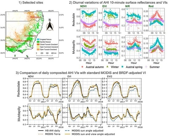
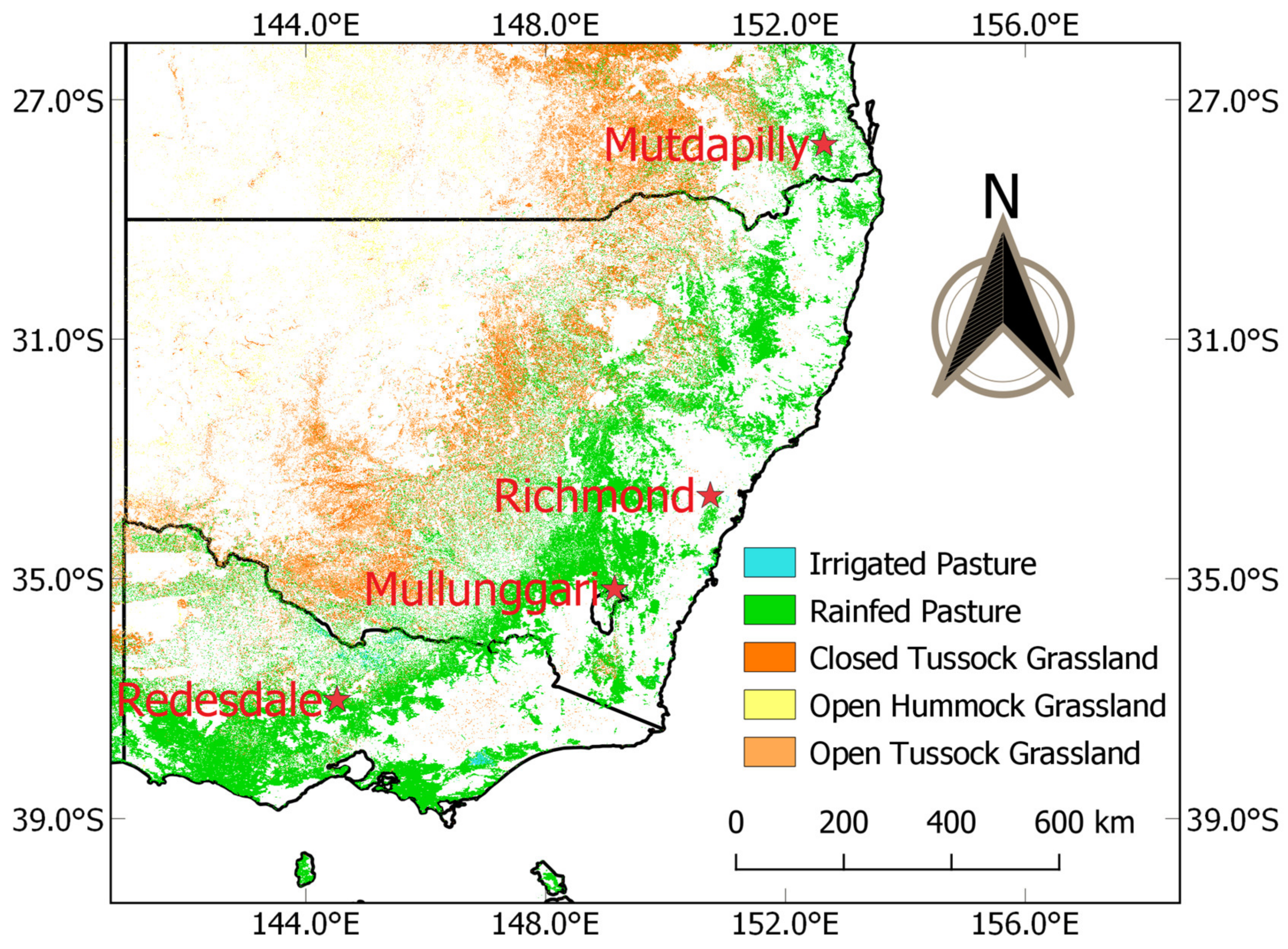
2.1. Study Sites

Four grassland sites along a subtropical to temperate latitudinal gradient in eastern Australia were selected for this study (Table 1, Figure 1). These sites encompass cool-season grasses at the higher latitudes, subtropical grasses at the lower latitudes, and mixed cool-season and warm-season grasses at the mid-latitude sites [28].

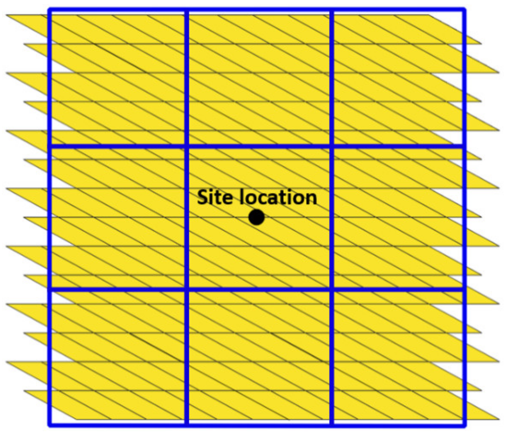
2.2. Himawari-8 AHI Data

Himawari-8 is a geostationary satellite launched on 7 October 2014 and is positioned at 140.7° E and 0.02° S [1]. The Advanced Himawari Imager (AHI) on-board the Himawari-8 satellite captures the full disc of the Asia–Pacific region every 10 minutes with spatial resolutions of 500 m for the red spectral band and 1000 m for all other visible/ near-infrared spectral bands [1] (Table 2). Given the Himawari-8 satellite fixed position near the Equator, the corresponding AHI view zenith angle (VZA) at the sites is uniquely fixed and ranged from 35.3° to 43.2° (Table 1). We aggregated the 500 m red band data to match the 1 km spatial resolution of the other bands.
Nearly two years of 10-min surface reflectance data were collected and processed by the Australian Bureau of Meteorology over the four grassland sites from March 2016 to December 2017. A 3 × 3 km extracted window was chosen to minimize the possible geolocation error of AHI, which was reported by Matsuoka [29]. Top-of-canopy directional surface reflectances were derived for the site specific view angle (Table 1, Figure 2) and 10-min intervals using the Multi-Angle Implementation of Atmospheric Correction (MAIAC) algorithm [30]. The MAIAC algorithm uses an advanced atmospheric correction algorithm with improved cloud detection and aerosol retrievals [30]. The sun-surface-sensor geometric orientation of the Himawari-8 AHI sensor is shown in Figure 2. The major steps involved AHI/ MODIS data extraction, BRDF correction, AHI daily compositing, and cross-sensor analyses are summarized in Figure 3.
An example of the diurnal and seasonal variations in solar zenith angle and sun-sensor relative azimuth angle is shown in Figure 4 for the highest latitude study site (Redesdale). Seasonally, solar zenith angles can range from 15° to 60° at solar noon, while diurnal ranges in solar zenith angle variations can be as extreme as 75° (austral summer) to 30° (austral winter). With the AHI sensor viewing southward, relative azimuthal angles range from approximately +90° at sunrise (east) to −90° (west), with the greatest seasonal variations occurring near sunrise and sunset, and minimal variations near solar noon (Figure 4). There were also solar zenith angle variations across the four latitudinal sites, as shown in Figure 5 for one specific time of the year (e.g., 1 July). Solar zenith angles at solar noon varied by 10° across the four sites, while relative azimuth angles were nearly invariant. These seasonal and diurnal SZA variations may potentially drive significant variations in surface reflectance and VIs [31,32].
Three vegetation indices (VIs) were computed and analyzed, including the normalized difference vegetation index (NDVI), the enhanced vegetation index (EVI), and the two-band enhanced vegetation index (EVI2) [33,34,35]. The equations defining these VIs are:
N D V I = ρ N I R ρ R E D ρ N I R + ρ R E D
E V I = 2.5 × ρ N I R ρ R E D ρ N I R + 6 × ρ R E D 7.5 × ρ B L U E + 1
E V I 2 = 2.5 × ρ N I R ρ R E D ρ N I R + 2.4 × ρ R E D + 1
where ρ N I R , ρ R E D , and ρ B L U E , are surface reflectances in the near-infrared, red, and blue bands, respectively. AHI has very similar spectral bands to MODIS in the blue, red, and NIR (Table 2).
The NDVI and EVI are standard products of the Terra and Aqua MODIS sensors and the follow-on Suomi VIIRS sensor [36]. The NDVI time series provide over 40 years of continuous greenness measures of vegetation dynamics over the entire globe [34]. EVI provides an optimized version of NDVI by reducing soil background and atmospheric influences [35]. The two-band EVI, or EVI2, was developed by Jiang for sensors without a blue band [33]. Furthermore, with ongoing improvements in atmosphere correction, the importance of the blue band in EVI is reduced. These VIs are widely used measures of canopy “greenness”, a combined property of green leaf cover, canopy structure, and chlorophyll content [37]. They are robust and provide seamless and consistent greenness measurements used for deriving vegetation biophysical and phenological parameters at regional to global scales [38,39,40,41].

2.3. Comparisons of MODIS VI Products with Himawari-8 AHI

In this study, Terra and Aqua MODIS standard VI products with 250 m spatial resolution (MOD13Q1 and MYD13Q1, version 6) were used for comparison with the Himawari-8 AHI VIs, along with their respective spectral reflectances used to derive the VIs [42]. We downloaded the MODIS data from the U.S. Geological Survey site (https://e4ftl01.cr.usgs.gov/). We also derived BRDF-adjusted reflectances [43] and VIs using the MODIS BRDF/ Albedo (MCD43A1) products for two key cases; (i) the MODIS reflectances and VIs were adjusted to local solar noon and nadir view zenith angles, and (ii) the MODIS reflectances and VIs were adjusted to both local solar noon and the native view angle of the Himawari-8 AHI sensor (Figure 3). In both MODIS BRDF adjustments, the relative azimuth angles (RAA) were set to those observed by AHI.
The MODIS BRDF product provides the modeled parameters needed to characterize the surface anisotropies resulting from variations in sun-sensor geometries. The product applies a semiempirical BRDF model called RossThick-LiSparse Reciprocal to model land surfaces as a combination of three parameters representing three scattering types: isotropic scattering, radiative transfer-type volumetric scattering, and geometric-optical surface scattering [22,30,44,45]. In this study, we used the latest version (version 6) of the MODIS BRDF/ Albedo product at 500 m scale to adjust and generate spectral reflectance and VIs to AHI native sun-sensor angles [46,47].
To match the different footprints between MODIS (polar orbiting) and AHI (geostationary) data, we sampled a 3 × 3 km window of 9 AHI pixels and extracted all available 250 m MODIS pixels, from March 2016 to December 2017, within the AHI footprint (Figure 3 and Figure 6). The average of 9 AHI pixels was compared with the average of all MODIS pixels within the AHI footprint. The Savitzky–Golay (SG) filter was applied to the MODIS VI time series datasets to minimize noise and outlier VI values [48].

2.4. Compositing Himawari-8 AHI VIs to Daily Values

We generated daily AHI reflectances and VIs from the 10-min data, by selecting cloud-free mid-day, near solar noon observations within a four-hour, 10–14 h, sampling period (Figure 3). The four-hour period was chosen to achieve a balance of higher data availability, smallest solar zenith angles, and minimal sun angle variations (mid-day sun angles will vary less than early morning and late afternoon). This also facilitated comparisons with MODIS VIs that were either adjusted to solar noon or were measured relatively close to solar noon, as with the standard Terra MOD13 products (10:30 a.m.) and Aqua MYD13 products (1:30 p.m.). A seventh-order median filter was used to remove spikes and outliers, and a Savitzky–Golay (SG) filter was applied to remove noise caused by subpixel clouds and residual atmospheric conditions [48].

3. Results

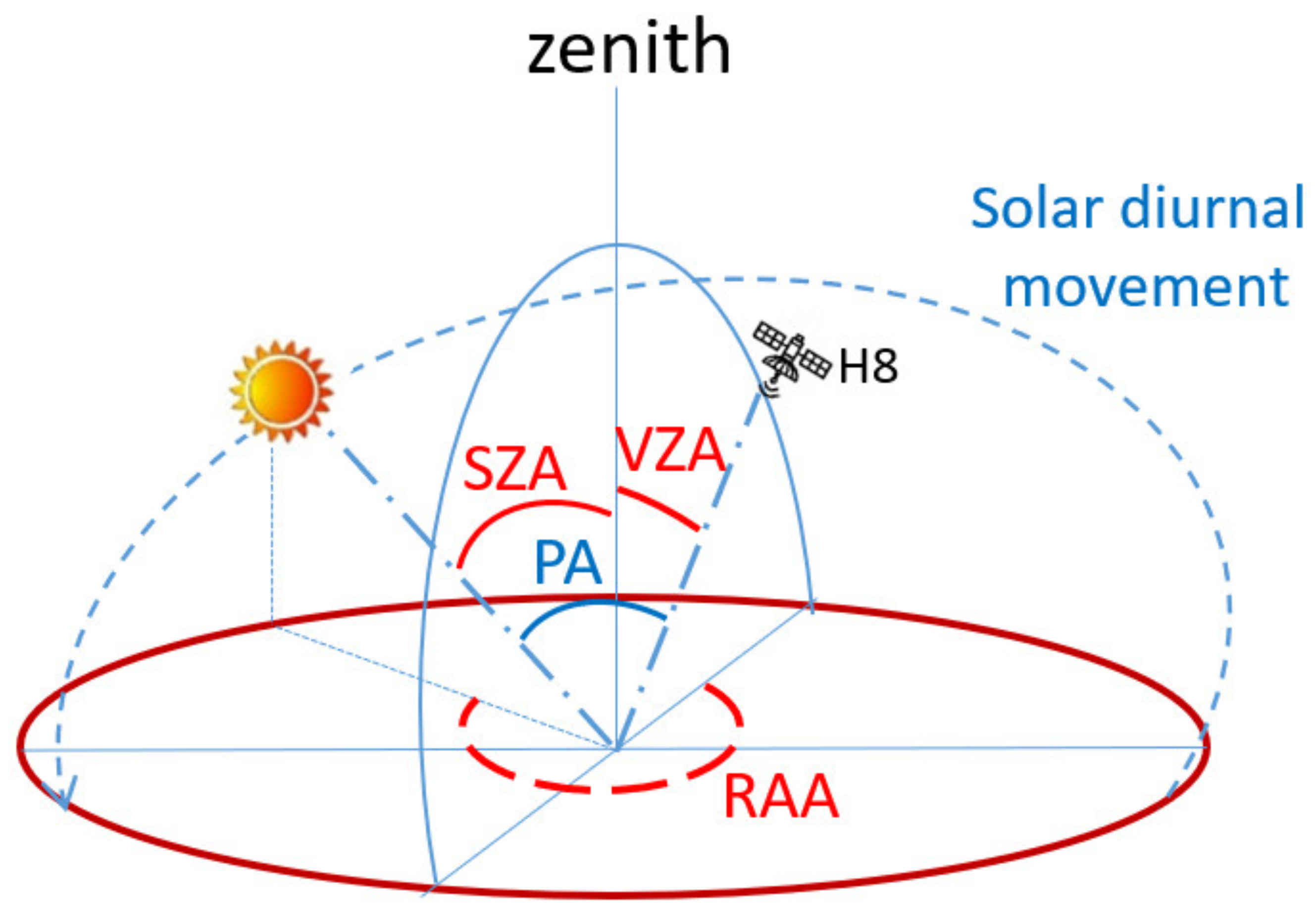
3.1. Diurnal Himawari-8 AHI VI Variations in Relation to Solar Zenith Angle Variations

Examples of complete 10-min time series of Himawari-8 AHI vegetation index values for the 2016 and 2017 growing seasons are illustrated in Figure 7 for the Redesdale grassland site. The seasonal profiles across the two growing seasons are representative of cool-season grasses, with green-up commencing in austral autumn (April), reaching peak activity in late winter/ austral spring (August–October), and end-of-growing season (brown-down) occurring in the summer (January). The color coded profiles reveal the diurnal range of solar zenith angles experienced and show significant AHI VI variations caused by sun angle related BRDF influences throughout the day (Figure 7). Overall, higher NDVI and EVI/ EVI2 values were found at the larger solar zenith angles encountered at the beginning and end of each day, with the lowest VI values occurring at the smallest solar zenith angles near local solar noon. The diurnal variations associated with sun angle were most distinct with NDVI and were present throughout the two grass growing seasons. On a daily basis, NDVI varied by approximately 0.20 units and EVI/ EVI2 by 0.15 units, which were equivalent to approximately 40% of their respective growing season amplitudes (Figure 7).
Diurnal sun angle influences on the VIs (NDVI, EVI, and EVI2), as well as the red, NIR, and blue reflectances were further investigated at four seasonal periods across all four study sites (Figure 8). The AHI red, blue, and NIR reflectances exhibited strong diurnal phase angle variations with their highest values occurring near solar noon and lowest values at the larger solar zenith angles, early and late in the day. NIR reflectances exhibited much weaker diurnal patterns relative to the red and blue reflectances (Figure 8). The derived AHI VI measures exhibited less pronounced but inverse diurnal patterns at all sites and seasonal periods, generally with the highest VI values at the beginning and end of each day (large solar zenith angle) and lowest values near mid-day, at solar noon sun angle conditions. The solar zenith angle influences mimic those shown in Figure 7 for the Redesdale site. The EVI and EVI2 diurnal patterns were much weaker than the NDVI profiles, and for most sites and seasonal periods approached a flat diurnal pattern.
A pronounced hotspot effect was observed mid-day near the austral autumn equinox period (end of March) and the austral spring equinox period (late September) at all grassland sites, when solar zenith angles approached the fixed view zenith angle of the AHI sensor in the backscatter direction. The high backscatter red reflectances and weaker backscatter NIR reflectances resulted in a negative NDVI hotspot effect. In contrast, the EVI and EVI2 were minimally affected by the hotspot.

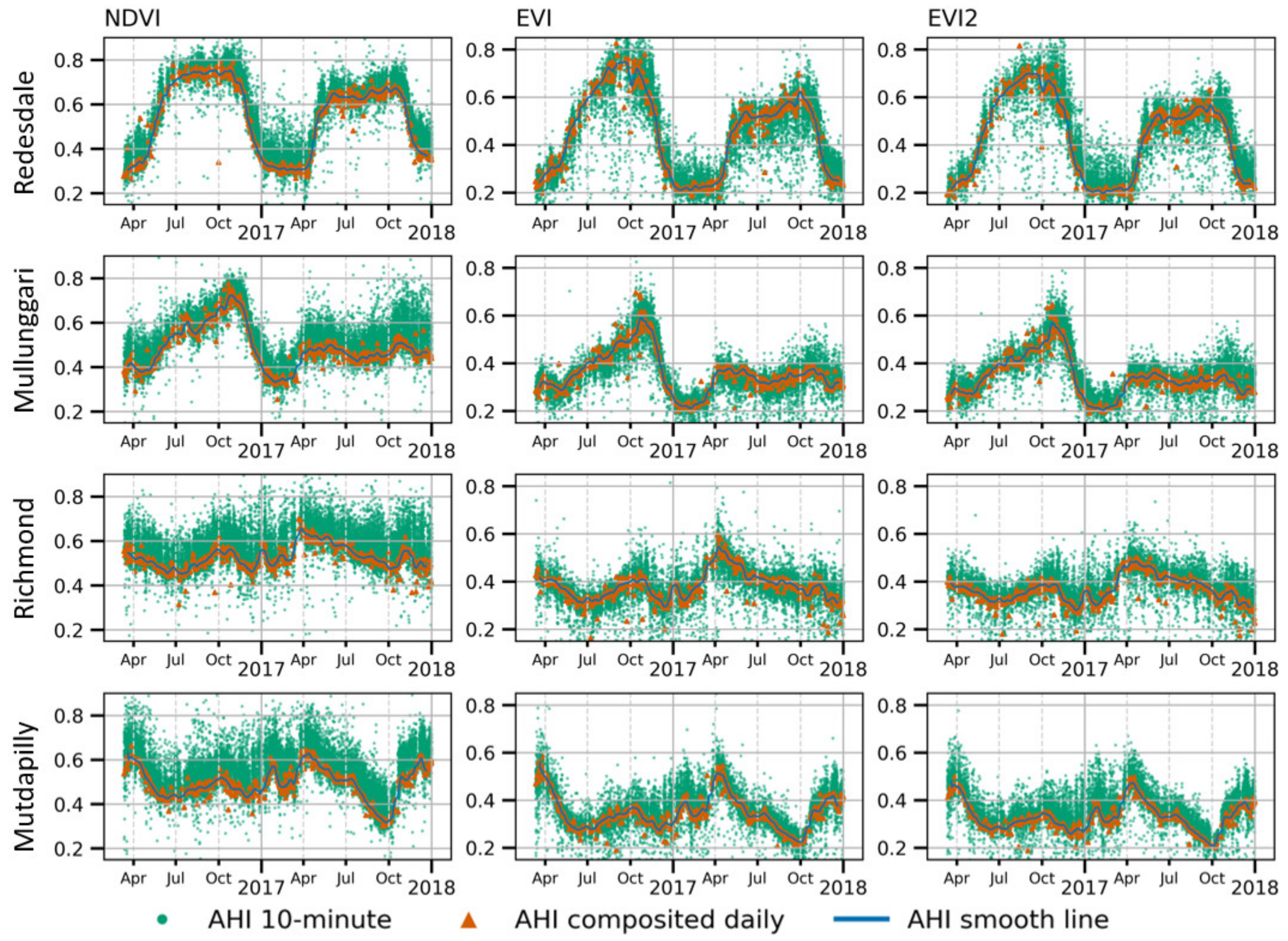
3.2. Seasonal Variations in Daily Composited Himawari-8 AHI VI Time Series

Daily composited Himawari-8 AHI NDVI and EVI2 values, derived from the local solar noon selection window (10–14 h) are shown in Figure 9 for all sites, along with the original 10-min data. The percentage of days that were successfully composited into daily AHI VI values were, on average 80% from the total time series of 661 days. The percentages from each site were similar, ranging from 78.2% at Redesdale to 81.7% at the Richmond site. The daily composited NDVI values followed the lower envelope of the 10-min NDVI data, consistent with the diurnal low NDVI values encountered around solar noon (Figure 8). The daily EVI and EVI2 values also plotted closer to the lower envelope of the 10-min data, however, not as tightly as with the NDVI, which was also consistent with the less pronounced diurnal EVI profiles (Figure 8 and Figure 9). Overall, the scatter of 10-min VI values was greatly reduced in the daily composited data. The remaining residual noise, probably associated with subpixel clouds and residual aerosol contamination, was further reduced by applying the Savitzky–Golay smoothing algorithm (blue line in Figure 9).

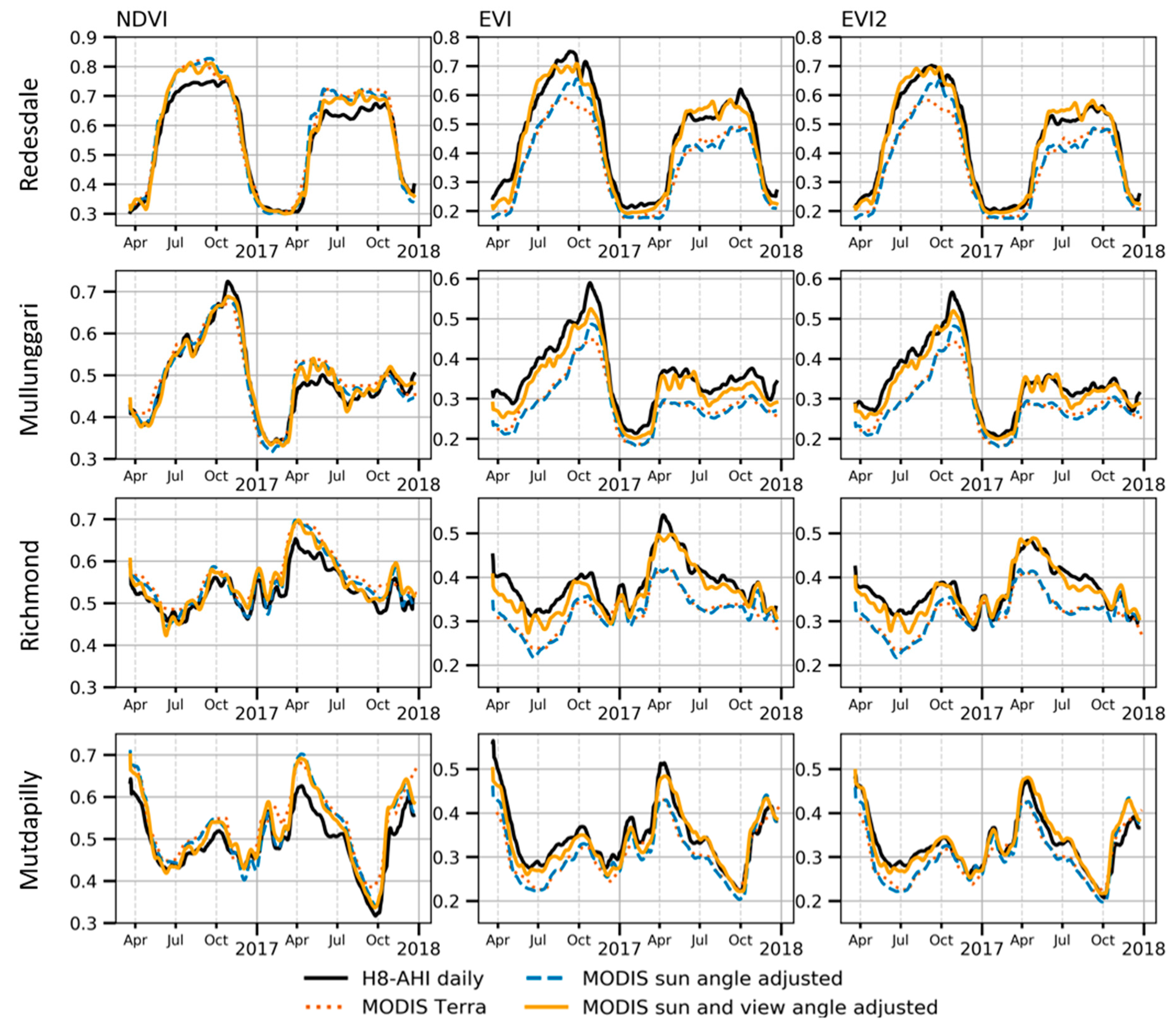
3.3. Seasonal Comparisons of Himawari-8 AHI and MODIS VIs

The Himawari-8 AHI daily composited VI seasonal profiles were compared with the Terra and Aqua MODIS standard VI products (MOD/ MYD13) at the Redesdale site (Figure 10a–c). The standard MODIS VI data generated similar NDVI, EVI, and EVI2 profile shapes as the AHI VIs, but with significant differences in their magnitudes. The MODIS NDVI profile was overall higher than AHI NDVI, while the MODIS EVI and EVI2 profiles were significantly lower than AHI EVI and EVI2 profiles. These magnitude differences were likely related to differences in AHI and MODIS cross-sensor observation geometries (Figure 10d–f). The AHI VIs were acquired at near solar noon sun zenith angles with a fixed oblique sensor view zenith angle (43°), while the MODIS VIs were observed at slightly larger solar zenith angles and view zenith angles between 0° to 30° (Figure 10d,e).
The two major cross-sensor observation geometry differences were (1) the more oblique sensor view zenith angle of AHI and (2) the smaller phase angles of AHI, relative to MODIS observations (Figure 10f). As the AHI phase angles were much lower than MODIS, particularly during the most active grass growing and peak greenness seasons, AHI observations were acquired under stronger backscatter orientations relative to MODIS during the same periods. The backscatter orientation of
AHI had a negative effect on NDVI values and a positive effect on EVI and EVI2 values, in agreement with a previous study [12]. Similar results were found in all four grassland areas (Table 3), in which MODIS NDVI values were consistently higher than AHI NDVI, and MODIS EVI and EVI2 values were consistently lower than AHI EVI and EVI2, respectively. On average, AHI NDVI was ~5% lower than MODIS NDVI, while AHI EVI was ~20% higher than MODIS EVI, and AHI EVI2 was ~15–20% higher than MODIS EVI2. Overall, AHI EVI values were slightly higher than EVI2, by about 5% with a mean difference of 0.02 units (Table 3).
Comparisons of the AHI VI time series with BRDF-adjusted (sun and view angle) MODIS data were analyzed to further explore the role of sun and view angle differences (Figure 11). Adjusting the MODIS MCD43 VI data to solar noon and nadir view resulted in only slight VI profile changes relative to the Terra MODIS VI product (Figure 11). Nevertheless, the solar noon adjusted MODIS NDVI values decreased slightly to better approximate the AHI NDVI, while solar noon adjusted MODIS EVI and EVI2 values increased to better approximate the respective AHI EVI/ EVI2 values (Table 3). These small differences reflect the small differences in seasonal SZA’s between the MODIS standard products and solar noon adjusted MODIS data at these grassland sites (Figure 10d).
Adjustment of the MODIS MCD43 VI data to solar noon and to the AHI fixed observation view angle resulted in stronger overall convergence of MODIS VI seasonal profiles with the AHI VI seasonal profiles (Figure 11, Table 4). The view angle adjustment had the effect of significantly increasing EVI/ EVI2 values, as much as 20%, and closely approximated the AHI EVI/ EVI2 values over all grassland sites. The sun and view angle adjusted MODIS EVI values were nearly identical to those of adjusted EVI2 values, however, AHI EVI values were consistently slightly higher than AHI EVI2 values (Figure 11) and the improvement of EVI was less significant relative to that of EVI2. View angle adjustments applied to the MODIS NDVI data had the effect of further lowering NDVI values to align more closely with AHI data (Figure 11). Overall, cross-sensor mean absolute differences between BRDF-corrected MODIS VIs (solar noon and fixed sensor view angle) with AHI VIs were lowest for EVI2 (0.014–0.019) when compared with NDVI (0.018–0.030) and EVI (0.018–0.31) (Table 4).

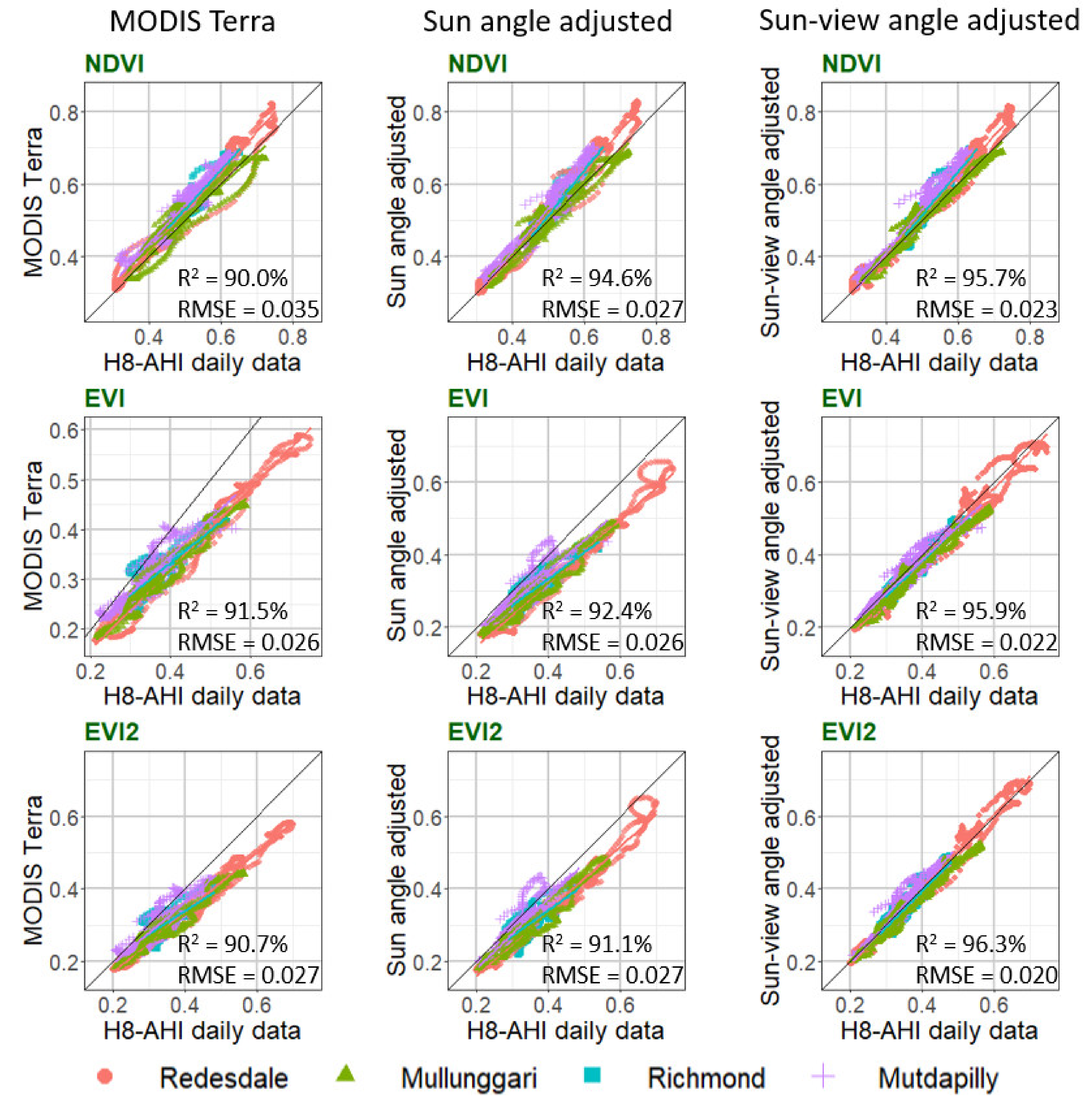
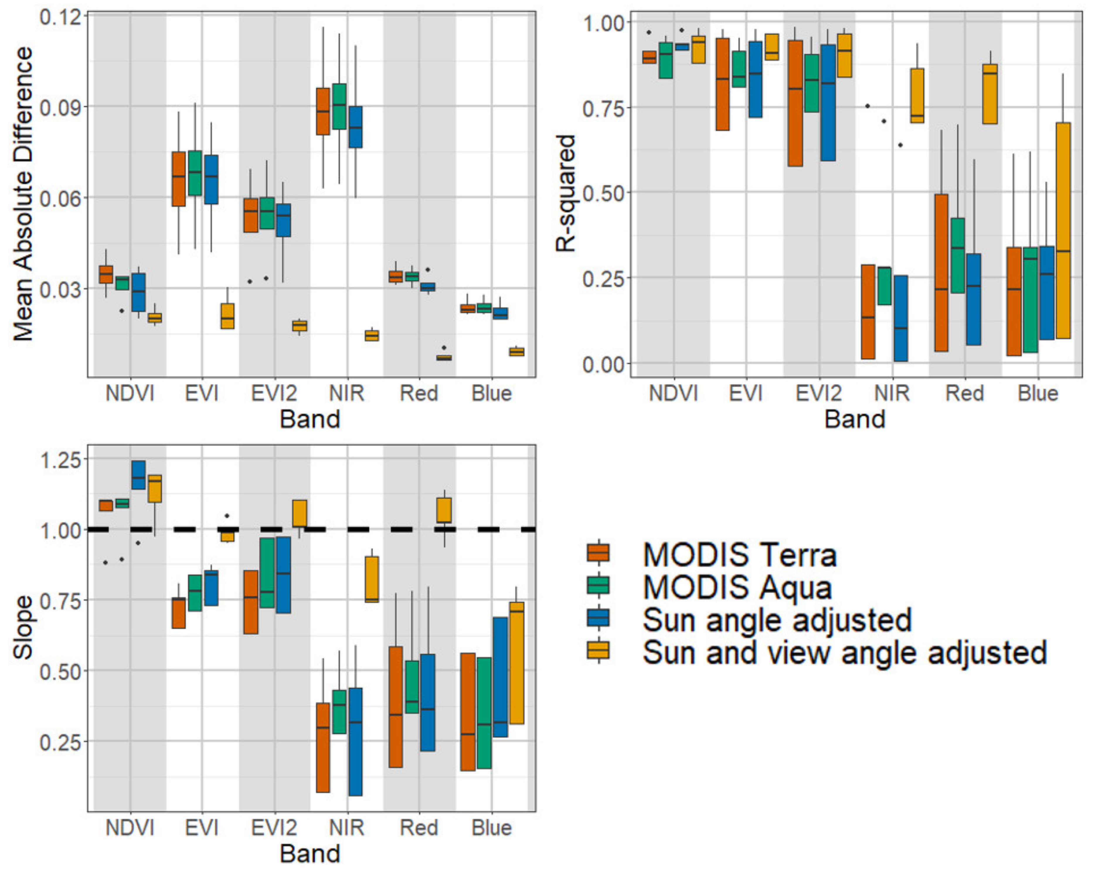
3.4. AHI and MODIS VI Relationships before and after Sun-View Geometry Adjustment

The cross-sensor relationships of AHI NDVI, EVI, and EVI2 values are plotted against the various MODIS sun and view angle adjusted NDVI, EVI, and EVI2 values in Figure 12. The global relationships using all four grassland sites significantly improved from AHI VI comparisons with standard Terra MODIS VIs (local sun angle) to the sun angle and view angle adjusted MODIS VIs (Figure 12). Using simple linear regression, the cross-sensor NDVI relationships improved by adjusting MODIS data to solar noon and nadir view (R2 increasing from 0.9 to 0.946) with a smaller increase when MODIS was adjusted to the AHI view angle (R2 = 0.957). Cross-sensor EVI and EVI2 relationships became more significant following solar noon and view angle adjustments with R2 increasing from 0.924 to 0.959 (EVI) and from 0.911 to 0.963 (EVI2) (Figure 12). The BRDF-adjustments also lowered RMSE values from 0.035 to 0.023 (NDVI), 0.026 to 0.022 (EVI), and 0.027 to 0.020 (EVI2), and all data points moved closer to the 1:1 line (Figure 12).
Lastly, global cross-sensor and cross-site relationships are shown in Figure 13 for NDVI, EVI, EVI2, and blue, red, and NIR surface reflectances. The mean absolute differences (MAD) in VI and reflectance values between the two sensors converged close to zero for all three VIs (<0.02) and three band reflectances (<0.015) from non-BRDF-adjusted to fully BRDF-adjusted MODIS VIs (Figure 13). The R2 values of the fitted linear regression function were significantly improved for all VIs and reflectances following complete BRDF adjustments, with R2 values exceeding 0.90 for all three VIs, and exceeding 0.8 for the red and NIR reflectances (Figure 13). The blue reflectance cross-sensor relationships performed the worst with R2 values of 0.50. The global relationship slopes show EVI and EVI2 converging toward slopes of 1 with BRDF-adjustments, while the NDVI increased to slope values slightly greater than 1 (1.1) with BRDF adjustments (Figure 13). Spectral reflectances converged toward slopes of 1, especially the red band, while the slope relationships were >0.8 for the NIR and >0.7 for the blue following BRDF adjustments.
Overall, EVI2 performed slightly better than EVI, which may be a consequence of the poor cross-sensor blue band relationships in terms of R2 and slope. Nevertheless, it is quite interesting that although the MODIS BRDF-adjusted reflectances did not agree as well with the AHI reflectances (slopes not as close to 1 and lower R2) when they were inserted into expressions of VIs, the cross-sensor VI comparisons were significantly improved with very little residual adjustment needed.

4. Discussion

Vegetation index seasonal profiles derived from different sensors are generally similar, as was found in this study. However, more detailed analyses can reveal important distinctions, which can result in systematic disparities when further processed to extract certain information (e.g., phenological metrics). Variations in cross-sensor VI profiles may be associated with differences in their spectral bandwidths, spatial and temporal resolutions, and observation geometries. Global VI products, including MODIS NDVI and EVI, GIMMS NDVI, and the current VIIRS VI products, are not normalized to a standard geometry with a BRDF-correction model, and instead rely on maximum value compositing (MVC) with quality analysis/ quality control (QA/ QC) and view angle constraints, [49,50,51]. Therefore, investigating and understanding how VI temporal profiles are different empirically with actual cross-sensor datasets is an important step to tackle, especially with the new generation of geostationary satellites, with unfamiliar observation geometries not experienced with MODIS, VIIRS, or AVHRR VI time series data.
The diurnal patterns of AHI VIs and reflectances over the four grassland study sites during four seasonal periods showed diverse phase angle driven BRDF effects that were VI and reflectance band dependent. Diurnal reflectances were very pronounced with maximum values sharply rising at solar noon, particularly with the blue and red bands. The diurnal reflectances were amplified by the hotspot effect, evident over spring and autumn equinox periods when sun zenith angles approached the AHI sensor view zenith angles in the backscatter direction. Whereas blue and red reflectances varied as much as two-fold near the hotspot periods, the NIR only increased by 33% during the same spring and autumn equinox periods. These differential cross-band sensitivities to diurnal phase angle changes resulted in strong NDVI diurnal variations, particularly near hotspot periods, where a negative NDVI hotspot effect resulted from the much greater positive red reflectances, relative to NIR reflectances [52,53,54]. In contrast EVI and EVI2 were nearly insensitive to diurnal phase angle variations and displayed nearly flat diurnal profiles without noticeable hotspot influences. Other studies have reported a positive hotspot effect on the EVI in evergreen and broadleaf forest canopies [54].
Overall, reflectances were highest during mid-day periods near solar noon, while VI values were lowest near solar noon. Similar diurnal VI patterns have been reported over partial grass canopy covers [23,32]. The results from the dry grassland sites studied here may not apply to other biomes. In another study, the extent of anisotropy in red and NIR reflectances and derived NDVI depended on the amount of vegetation present, with maximum anisotropies at ~50% canopy cover [55]. The directional diurnal patterns may further vary with canopy architecture, and leaf and soil optical properties. Over structurally complex land cover types, such as woodlands and forests, diurnal patterns will further be influenced by shaded and sunlit forest canopy components and intercrown shadowing [25,32,53,56].
Our diurnal results contrast with studies where top-of-atmosphere (TOA) reflectances were used and diurnal VI values were driven by atmosphere influences (path length), in which maximum VI values occurred mid-day (noon time) when there was less atmosphere scattering of sunlight [5,13].
Daily compositing methodologies based on maximum VI values would thus minimize atmosphere influences and reduce cloud contamination. In this study, the atmosphere-corrected data brought about BRDF influences to drive diurnal VI and reflectance variations, and maximum value compositing (MVC) would no longer be applicable since the highest VI values may occur at the largest sun zenith angles, near sunrise and sunset periods. In our compositing, we selected minimum VI values near solar noon, which made it more difficult to filter out residual cloud and aerosol contamination that also lowers VI values. For this study we widened the mid-day compositing window from 10 to 14 h and used a Savitzky–Golay (SG) filter to help reduce atmosphere noise.
For seasonal scale analysis, we used daily AHI composited VI values constrained to mid-day (10–14 h) to enable comparisons with the sun angle conditions experienced by Terra (10:30 a.m.) and Aqua (1:30 p.m.) MODIS VIs. Despite the oblique view zenith angles of AHI (35° to 43°), seasonal AHI NDVI values were lower than MODIS NDVI values. With the high sensitivity of NDVI to sun angle found in all growing season periods, one would expect a higher, not lower, NDVI with larger view zenith angle. This diurnal to seasonal apparent inconsistency was also found in the EVI/ EVI2 cross-sensor comparisons. Although AHI EVI/ EVI2 values were insensitive to diurnal solar zenith angles, the AHI EVI/ EVI2 values, from larger view zenith angles, were higher relative to MODIS values. We attribute these cross-sensor differences in VI patterns to the year-round smaller phase angles and backscatter observations from AHI, in which the sunlit canopies induced a positive EVI/ EVI2 response and negative NDVI response (as a NDVI negative hotspot effect). The negative AHI NDVI backscatter response more than offset what should have been a positive AHI view angle response. These unique VI responses to sun-sensor phase angle, whereby NDVI is higher in the shaded, forward scattering direction, while EVI is higher in the sunlit, backscatter direction have previously been reported [53,54]. There was also a possibility of NDVI saturation issues, as three of the four sites had high NDVI values reaching over 0.7 (Figure 11) [35].
The improved cross-sensor relationships obtained between the AHI VI and MODIS VI time-series following BRDF adjustments of the MODIS data highlight both the potential compatibility between AHI and MODIS data as well as the importance of BRDF corrections to minimize cross-sensor, sun-view geometry differences. Our comparisons would be much less accurate if we had used AHI solar zenith angles beyond those observed by MODIS. We further limited the BRDF modeled MODIS data to approximate the fixed view zenith angle and solar noon conditions of our composited daily AHI data. Compatibility between AHI and MODIS VI data, after applying BRDF correction, offers the potential of data gap filling MODIS VI data as well as conduct finer resolution phenology studies. Standardizing sun-sensor geometrical differences would be a key critical step to achieve these capabilities.
EVI2 was found to exhibit better cross-sensor correlations than EVI, suggesting the blue band may be introducing more noise to the relationships. The cross-sensor regression relationship of the blue band was very low, even after applying a full BRDF correction (R2 of 0.3). The equivalent relationships of the red and NIR bands were R2 of 0.8 and 0.7, respectively (Figure 13). A recent study by Li showed similar discrepancies of blue band reflectances between AHI and MODIS Terra/ Aqua [6], and other AHI studies using TOA reflectances also chose EVI2 over EVI [5,17]. The mismatching of blue band reflectances between MODIS and AHI may relate to the greater atmosphere path length of AHI data (VZA > 40°) and the sensitivity of the blue band to aerosols and subpixel clouds.
New operational methods for compositing geostationary data may need more careful consideration. Empirically, one could normalize AHI diurnal solar zenith angle variations to solar noon as was done in this study; however, seasonal sun angle variations would remain that spatially vary with latitude. AHI will still have significant oblique viewing geometries that would not be easy to harmonize with a polar orbiting sensor, such as MODIS, without a physical BRDF correction implemented to adjust AHI data to a nadir view angle, or to adjust MODIS data to the AHI view angle observation. Thus, a complete BRDF correction for view and sun angle conditions to a reference fixed view zenith angle and reference fixed solar zenith angle may be needed for global harmonization [57,58].
BRDF-based compositing methods would be preferred over empirical maximum value compositing methods. The MAIAC algorithm may soon offer a complete atmosphere and BRDF correction for geostationary sensors, hence standardizing all GEO measurements to a fixed view and sun angle [6,30]. However, such fixed sun-sensor geometric conditions will invariably result in modeled VI values that fall outside the range of real measurements for significant spatial geographic areas and periods of the year. More research would be needed to optimize the configuration of a global, standard sun-view geometry for GEO observations.
The grassland sites selected for this study cover a wide range of functional and species composition and represent a biome of high importance in Australia. These grasslands respond quickly to rainfall and climate extremes, and thus exhibit very dynamic growing patterns that make them excellent areas for high resolution monitoring. From a phenological perspective, both AHI VIs successfully discriminated the subtropical, warm-season grasses from the temperate, cool-season grasses along the latitudinal gradient. The two higher latitude sites exhibited strong, cool-season grass, October peaks (austral spring), while the two lower latitude sites show stronger warm-season grass peaks in April (austral autumn) (Figure 11). Furthermore, the multiple flowering cycles typically found in subtropical grass species, as in the Richmond and Mutdapilly sites, could be observed in the AHI VI data and to some extent in the MODIS data over the summer to austral autumn period (January–April) (Figure 11). In the case of MODIS data, it is difficult to confirm such fine biologic signals and distinguish them from noise related artifact signals or QA issues; hence the finer scale detail offered by AHI VI data will help resolve such fine scale phenology features.
Our study only investigated the similarity between AHI and MODIS data at grassland sites. As the BRDF impact is complex and dependent on both varying sun-sensor geometries and canopy structures, future investigations should be conducted for other landscapes like croplands, forests, and other locations such as areas near the Equator where AHI view zenith angles are close to nadir. There are also other cross-sensor issues that need to be considered, including discrepancies resulting from different pixel footprints, AHI registration issues, calibration, different atmosphere correction methods (MAIAC vs. MOD09), and differences in cloud masking methods and resolution. Investigating BRDF influences, as done here, is nevertheless a major step forward and appears to be the dominant driver of cross-sensor variations between Himwari-8 AHI VIs and MODIS VIs.

5. Conclusions

Geostationary satellite sensors such as Himawari-8 AHI potentially offer improved science quality data for monitoring landscapes and diagnosing phenology at very high temporal resolution. Compatibility in VI values between AHI and polar orbiting satellite sensor data would be useful for many earth observing applications. In this study we investigated diurnal and seasonal NDVI, EVI, and EVI2 patterns under AHI oblique year-round backscatter view orientations. We further analyzed the cross-sensor dependencies of observation geometries on the compatibility between AHI and MODIS vegetation indices. After compositing the 10-min AHI data to daily values centered on solar noon sun angles, we found both view zenith and phase angle differences between AHI and MODIS to be strong drivers of cross-sensor VI differences. The backscatter view direction of AHI at solar noon resulted in unique and opposite NDVI and EVI/ EVI2 responses relative to the observed MODIS VIs, across our four grassland study sites.
Our results highlight the relevance of cross-sensor sun-view geometries in order to harmonize AHI and MODIS annual time series. The AHI solar noon compositing minimized the large range of solar zenith angle variations present in the AHI diurnal data and approximated the nominal Terra and Aqua MODIS sun angles. The strong agreement found in this study following BRDF-corrections, shows promise in cross-sensor applications and suggests that a denser time series can be formed through combined GEO and LEO measurement synergies. This has great potential for improved monitoring of highly dynamic grasslands and fine-scale retrievals of grassland phenology.

Author Contributions

N.N.T. and A.H. conceived the conceptualization, designed the experiments, and prepared the manuscript. H.N. provided scientific guidance and helped with data curation. E.E., I.G., T.M., X.M., Y.W., and A.L. contributed with writing and editing of the manuscript. All authors have read and agreed to the published version of the manuscript.

Funding

This research was funded by the Victorian Department of Health and Human Services with support from the Bureau of Meteorology. Additional support was provided from an NHMRC AusPollen Partnership (GNT1116107) led by Professor Janet Davies (Queensland University of Technology) and an Australia Research Council (ARC) Discovery Project (DP170101630) led by Professor Alfredo Huete (University of Technology Sydney). The work of A. Lyapustin and Y. Wang was funded by the NASA Science of Terra, Aqua, and SNPP programs (17-TASNPP17-0116; solicitation NNH17ZDA001NTASNPP). The work of T. Miura was funded by the NASA Terra program (80NSSC19K1691). X. Ma received a “Research Startup Funding for Youth Professor (2019-2024)” granted by Lanzhou University.

Acknowledgments

The authors would like to thank Leon Majewski from Australia Bureau of Meteorology for his processing of raw Himawari-8 data. Computational facilities were provided by the UTS eResearch High Performance Computer Cluster (UTS HPCC).

Conflicts of Interest

The authors declare no conflict of interest. The funders had no role in the design of the study; in the collection, analyses, or interpretation of data; in the writing of the manuscript, or in the decision to publish the results.

References

  1. Bessho, K.; Date, K.; Hayashi, M.; Ikeda, A.; Imai, T.; Inoue, H.; Kumagai, Y.; Miyakawa, T.; Murata, H.; Ohno, T.; et al. An introduction to Himawari-8/9 — Japan’s new-generation geostationary meteorological satellites. J. Meteorol. Soc. Jpn. 2016, 94, 151–183. [Google Scholar] [CrossRef] [Green Version]
  2. Choi, Y.S.; Ho, C.H. Earth and environmental remote sensing community in South Korea: A review. Remote Sens. Appl. Soc. Environ. 2015, 2, 66–76. [Google Scholar] [CrossRef]
  3. Goodman, S.J. GOES-R Series Introduction. The GOES-R Series: A New Generation of Geostationary Environmental Satellites; Elsevier: Amsterdam, The Netherlands, 2019; pp. 1–3. [Google Scholar]
  4. Zhang, P.; Zhu, L.; Tang, S.; Gao, L.; Chen, L.; Zheng, W.; Han, X.; Chen, J.; Shao, J. General comparison of FY-4A/AGRI with other GEO/LEO instruments and its potential and challenges in non-meteorological applications. Front. Earth Sci. 2019, 6, 1–13. [Google Scholar] [CrossRef] [Green Version]
  5. Miura, T.; Nagai, S.; Takeuchi, M.; Ichii, K.; Yoshioka, H. Improved Characterisation of Vegetation and Land Surface Seasonal Dynamics in Central Japan with Himawari-8 Hypertemporal Data. Sci. Rep. 2019, 9, 1–12. [Google Scholar]
  6. Li, S.; Wang, W.; Hashimoto, H.; Xiong, J.; Vandal, T.; Yao, J.; Qian, L.; Ichii, K.; Lyapustin, A.; Wang, Y.; et al. First provisional land surface reflectance product from geostationary satellite Himawari-8 AHI. Remote Sens. 2019, 11, 1–12. [Google Scholar] [CrossRef] [Green Version]
  7. Fensholt, R.; Ayamba, A.; Stisen, S.; Sandholt, I.; Pak, E.; Small, J. Comparisons of compositing period length for vegetation index data from polar-orbiting and geostationary satellites for the cloud-prone region of West Africa. Photogramm. Eng. Remote Sens. 2007, 73, 297–309. [Google Scholar] [CrossRef]
  8. Guan, K.; Medvigy, D.; Wood, E.F.; Caylor, K.K.; Li, S.; Jeong, S.J. Deriving vegetation phenological time and trajectory information over africa using seviri daily LAI. Ieee Trans. Geosci. Remote Sens. 2014, 52, 1113–1130. [Google Scholar] [CrossRef]
  9. Yan, D.; Zhang, X.; Yu, Y.; Guo, W. A Comparison of Tropical Rainforest Phenology Retrieved from Geostationary (SEVIRI) and Polar-Orbiting (MODIS) Sensors Across the Congo Basin. Ieee Trans. Geosci. Remote Sens. 2016, 54, 4867–4881. [Google Scholar] [CrossRef] [Green Version]
  10. Chen, Y.; Sun, K.; Chen, C.; Bai, T.; Park, T.; Wang, W.; Nemani, R.R.; Myneni, R.B. Generation and evaluation of LAI and FPAR products from Himawari-8 advanced Himawari imager (AHI) data. Remote Sens. 2019, 11. [Google Scholar] [CrossRef] [Green Version]
  11. He, T.; Zhang, Y.; Liang, S.; Yu, Y. Developing Land Surface Directional Reflectance and Albedo Products from Geostationary GOES-R and Himawari Data: Theoretical Basis, Operational Implementation, and Validation. Remote Sens. 2019, 1–21. [Google Scholar] [CrossRef] [Green Version]
  12. Adachi, Y.; Kikuchi, R.; Obata, K.; Yoshioka, H. Relative azimuthal-angle matching (RAM): A screening method for GEO-LEO reflectance comparison in middle latitude forests. Remote Sens. 2019, 11. [Google Scholar] [CrossRef] [Green Version]
  13. Wheeler, K.I.; Dietze, M.C. A statistical model for estimating Midday NDVI from the Geostationary Operational Environmental Satellite (GOES) 16 and 17. Remote Sens. 2019, 11. [Google Scholar] [CrossRef] [Green Version]
  14. Fensholt, R.; Sandholt, I.; Stisen, S.; Tucker, C. Analysing NDVI for the African continent using the geostationary meteosat second generation SEVIRI sensor. Remote Sens. Environ. 2006, 101, 212–229. [Google Scholar] [CrossRef]
  15. Sobrino, J.A.; Julien, Y.; Soria, G. Phenology estimation from meteosat second generation data. IEEE J. Sel. Top. Appl. Earth Obs. Remote Sens. 2013, 6, 1653–1659. [Google Scholar] [CrossRef]
  16. Fang, L.; Zhan, X.; Schull, M.; Kalluri, S.; Laszlo, I.; Yu, P.; Carter, C.; Hain, C.; Anderson, M. Evapotranspiration data product from NESDIS GET-D system upgraded for GOES-16 ABI observations. Remote Sens. 2019, 11. [Google Scholar] [CrossRef] [Green Version]
  17. Yan, D.; Zhang, X.; Nagai, S.; Yu, Y.; Akitsu, T.; Nasahara, K.N.; Ide, R.; Maeda, T. Evaluating land surface phenology from the Advanced Himawari Imager using observations from MODIS and the Phenological Eyes Network. Int. J. Appl. Earth Obs. Geoinf. 2019, 79, 71–83. [Google Scholar] [CrossRef]
  18. Sobrino, J.A.; Julien, Y. Trend Analysis of Global MODIS-Terra Vegetation Indices and Land Surface Temperature Between 2000 and 2011. Ieee J. Sel. Top. Appl. Earth Obs. Remote Sens. 2013, 6, 2139–2145. [Google Scholar] [CrossRef]
  19. Yan, D.; Zhang, X.; Yu, Y.; Guo, W.; Hanan, N.P. Characterizing land surface phenology and responses to rainfall in the Sahara desert. J. Geophys. Res. Biogeosciences 2016, 121, 2243–2260. [Google Scholar] [CrossRef] [Green Version]
  20. Qin, Y.; McVicar, T.R. Spectral band unification and inter-calibration of Himawari AHI with MODIS and VIIRS: Constructing virtual dual-view remote sensors from geostationary and low-Earth-orbiting sensors. Remote Sens. Environ. 2018, 209, 540–550. [Google Scholar] [CrossRef]
  21. Purbantoro, B.; Aminuddin, J.; Manago, N.; Toyoshima, K.; Lagrosas, N.; Sumantyo, J.T.S.; Kuze, H. Comparison of aqua/terra MODIS and Himawari-8 satellite data on cloud mask and cloud type classification using split window algorithm. Remote Sens. 2019, 11, 1–19. [Google Scholar] [CrossRef] [Green Version]
  22. Roujean, J.-L.; Leroy, M.; Deschamps, P.-Y. A bidirectional reflectance model of the Earth’s surface for the correction of remote sensing data. J. Geophys. Res. 1992, 97, 20455. [Google Scholar] [CrossRef]
  23. Middleton, E.M. Solar zenith angle effects on vegetation indices in tallgrass prairie. Remote Sens. Environ. 1991, 38, 45–62. [Google Scholar] [CrossRef]
  24. Ma, X.; Huete, A.; Tran, N.N. Interaction of seasonal sun-angle and savanna phenology observed and modelled using MODIS. Remote Sens. 2019, 11, 1–19. [Google Scholar] [CrossRef] [Green Version]
  25. Morton, D.C.; Nagol, J.; Carabajal, C.C.; Rosette, J.; Palace, M.; Cook, B.D.; Vermote, E.F.; Harding, D.J.; North, P.R.J. Amazon forests maintain consistent canopy structure and greenness during the dry season. Nature 2014, 506, 221–224. [Google Scholar] [CrossRef]
  26. Sims, D.A.; Rahman, A.F.; Vermote, E.F.; Jiang, Z. Seasonal and inter-annual variation in view angle effects on MODIS vegetation indices at three forest sites. Remote Sens. Environ. 2011, 115, 3112–3120. [Google Scholar] [CrossRef]
  27. Bhandari, S.; Phinn, S.; Gill, T. Assessing viewing and illumination geometry effects on the MODIS vegetation index (MOD13Q1) time series: implications for monitoring phenology and disturbances in forest communities in Queensland, Australia. Int. J. Remote Sens. 2011, 32, 7513–7538. [Google Scholar] [CrossRef]
  28. Medek, D.E.; Beggs, P.J.; Erbas, B.; Jaggard, A.K.; Campbell, B.C.; Vicendese, D.; Johnston, F.H.; Godwin, I.; Huete, A.R.; Green, B.J.; et al. Regional and seasonal variation in airborne grass pollen levels between cities of Australia and New Zealand. Aerobiol. (Bologna). 2016, 32, 289–302. [Google Scholar] [CrossRef]
  29. Matsuoka, M.; Honda, R.; Nonomura, A.; Moriya, H.; Akatsuka, S.; Yoshioka, H.; Takagi, M. A method to improve geometric accuracy of Himawari-8/AHI “Japan Area” data. J. Jpn. Soc. Photogramm. Remote Sens 2016, 54, 280–289. [Google Scholar]
  30. Lyapustin, A.I.; Wang, Y.; Laszlo, I.; Hilker, T.; Hall, G.F.; Sellers, P.J.; Tucker, C.J.; Korkin, S.V. V. Multi-angle implementation of atmospheric correction for MODIS (MAIAC): 3. Atmospheric correction. Remote Sens. Environ. 2012, 127, 385–393. [Google Scholar] [CrossRef]
  31. Ishihara, M.; Inoue, Y.; Ono, K.; Shimizu, M.; Matsuura, S. The impact of sunlight conditions on the consistency of vegetation indices in croplands-Effective usage of vegetation indices from continuous ground-based spectral measurements. Remote Sens. 2015, 7, 14079–14098. [Google Scholar] [CrossRef] [Green Version]
  32. Ma, X.; Huete, A.; Tran, N.N.; Bi, J.; Gao, S.; Zeng, Y. Sun-Angle Effects on Remote-Sensing Phenology Observed and Modelled Using Himawari-8. Remote Sens. 2020, 12, 1339. [Google Scholar] [CrossRef] [Green Version]
  33. Jiang, Z.; Huete, A.R.; Didan, K.; Miura, T. Development of a two-band enhanced vegetation index without a blue band. Remote Sens. Environ. 2008, 112, 3833–3845. [Google Scholar] [CrossRef]
  34. Rouse, J.W.; Hass, R.H.; Schell, J.A.; Deering, D.W. Monitoring vegetation systems in the great plains with ERTS. Third Earth Resour. Technol. Satell. Symp. 1973, 1, 309–317. [Google Scholar]
  35. Huete, A.; Didan, K.; Miura, T.; Rodriguez, E.P.; Gao, P.; Ferreira, L.G. Overview of the radiometric and biophysical performance of the MODIS vegetation indices. Remote Sens. Environ. 2002, 83, 195–213. [Google Scholar] [CrossRef]
  36. Jarchow, C.J.; Didan, K.; Barreto-Muñoz, A.; Nagler, P.L.; Glenn, E.P. Application and comparison of the MODIS-derived enhanced vegetation index to VIIRS, landsat 5 TM and landsat 8 OLI platforms: A case study in the arid colorado river delta, Mexico. Sensors 2018, 18. [Google Scholar] [CrossRef] [Green Version]
  37. Myneni, R.B.; Hall, F.G.; Sellers, P.J.; Marshak, A.L. The interpretation of spectral vegetation indices. IEEE Trans. Geosci. Remote Sens. 1995, 33, 481–486. [Google Scholar] [CrossRef]
  38. Zhang, X.; Friedl, M.A.; Schaaf, C.B.; Strahler, A.H.; Hodges, J.C.F.; Gao, F.; Reed, B.C.; Huete, A. Monitoring vegetation phenology using MODIS. Remote Sens. Environ. 2003, 84, 471–475. [Google Scholar] [CrossRef]
  39. De Beurs, K.M.; Henebry, G.M. Spatio-Temporal Statistical Methods for Modelling Land Surface Phenology. In Phenological Research: Methods for Environmental and Climate Change Analysis; Hudson, I.L., Keatley, M.R., Eds.; Springer: Dordrecht, UK, 2010; pp. 177–208. ISBN 978-90-481-3334-5. [Google Scholar]
  40. Jeganathan, C.; Dash, J.; Atkinson, P.M. Remotely sensed trends in the phenology of northern high latitude terrestrial vegetation, controlling for land cover change and vegetation type. Remote Sens. Environ. 2014, 143, 154–170. [Google Scholar] [CrossRef]
  41. Broich, M.; Huete, A.; Paget, M.; Ma, X.; Tulbure, M.; Coupe, N.R.; Evans, B.; Beringer, J.; Devadas, R.; Davies, K.; et al. A spatially explicit land surface phenology data product for science, monitoring and natural resources management applications. Environ. Model. Softw. 2015, 64, 191–204. [Google Scholar] [CrossRef]
  42. Didan, K. MOD13Q1 MODIS/Terra Vegetation Indices 16-Day L3 Global 250m SIN Grid V006 [Data set] 2015. MOD13Q1 v006. Available online: https://doi.org/10.5067/MODIS/MOD13Q1.006 (accessed on 2 August 2020).
  43. Vermote, E.; Justice, C.O.; Breon, F.M. Towards a Generalized Approach for Correction of the BRDF Effect in MODIS Directional Reflectances. IEEE Trans. Geosci. Remote Sens. 2009, 47, 898–908. [Google Scholar] [CrossRef]
  44. Strahler, A.H.; Muller, J.P. MODIS BRDF Albedo Product: Algorithm Theoretical Basis Document. Vesion 5. 1999; pp. 1–53. Available online: https://modis.gsfc.nasa.gov/data/atbd/atbd_mod09.pdf (accessed on 22 June 2020).
  45. Schaaf, C.B.; Gao, F.; Strahler, A.H.; Lucht, W.; Li, X.; Tsang, T.; Strugnell, N.C.; Zhang, X.; Jin, Y.; Muller, J.P.; et al. First operational BRDF, albedo nadir reflectance products from MODIS. Remote Sens. Environ. 2002, 83, 135–148. [Google Scholar] [CrossRef] [Green Version]
  46. Schaaf, C.; Wang, Z. MCD43A1 MODIS/Terra+Aqua BRDF/Albedo Model Parameters Daily L3 Global - 500m V006 2015. MCD43A1 v006. Available online: https://doi.org/10.5067/MODIS/MCD43A1.006 (accessed on 2 August 2020).
  47. Strahler, A.; Gopal, S.; Lambin, E.; Moody, A. MODIS Land Cover Product Algorithm Theoretical Basis Document ( ATBD ) MODIS Land Cover and Land-Cover Change. Change 1999, 72. [Google Scholar]
  48. Savitzky, A.; Golay, M.J.E. Smoothing and Differentiation of Data by Simplified Least Squares Procedures. Anal. Chem. 1964, 36, 1627–1639. [Google Scholar] [CrossRef]
  49. Didan, K.; Munoz, A.B.; Huete, A. MODIS Vegetation Index User ’ s Guide ( MOD13 Series ). 2015. Available online: https://vip.arizona.edu/documents/MODIS/MODIS_VI_UsersGuide_June_2015_C6.pdf (accessed on 22 June 2020).
  50. Vargas, M.; Miura, T.; Shabanov, N.; Kato, A. An initial assessment of Suomi NPP VIIRS vegetation index EDR. J. Geophys. Res. Atmos. 2013, 118, 12,301–12,316. [Google Scholar] [CrossRef] [Green Version]
  51. Pinzon, J.E.; Tucker, C.J. A non-stationary 1981-2012 AVHRR NDVI3g time series. Remote Sens. 2014, 6, 6929–6960. [Google Scholar] [CrossRef] [Green Version]
  52. Gao, F.; Jin, Y.; Li, X.; Schaaf, C.B.; Strahler, A.H. Bidirectional NDVI and atmospherically resistant BRDF inversion for vegetation canopy. Ieee Trans. Geosci. Remote Sens. 2002, 40, 1269–1278. [Google Scholar]
  53. Leblanc, S.C.; Chen, J.M.; Cihlar, J. Ndvi directionality in boreal forests: A model interpretation of measurements. Can. J. Remote Sens. 1997, 23, 369–380. [Google Scholar] [CrossRef]
  54. Zhang, X.; Qiu, F.; Zhan, C.; Zhang, Q.; Li, Z.; Wu, Y.; Huang, Y.; Chen, X. Acquisitions and applications of forest canopy hyperspectral imageries at hotspot and multiview angle using unmanned aerial vehicle platform. J. Appl. Remote Sens. 2020, 14, 1–16. [Google Scholar] [CrossRef]
  55. Fensholt, R.; Sandholt, I.; Proud, S.R.; Stisen, S.; Rasmussen, M.O. Assessment of MODIS sun-sensor geometry variations effect on observed NDVI using MSG SEVIRI geostationary data. Int. J. Remote Sens. 2010, 31, 6163–6187. [Google Scholar] [CrossRef]
  56. Li, X.; Strahler, A.H. Geometric-optical bidirectional reflectance modeling of the discrete crown vegetation canopy: effect of crown shape and mutual shadowing. Ieee Trans. Geosci. Remote Sens. 1992, 30, 276–292. [Google Scholar] [CrossRef]
  57. Bréon, F.M.; Vermote, E. Correction of MODIS surface reflectance time series for BRDF effects. Remote Sens. Environ. 2012, 125, 1–9. [Google Scholar] [CrossRef]
  58. Middleton, E.M. Quantifying reflectance anisotropy of photosynthetically active radiation in grasslands. J. Geophys. Res. Atmos. 1992, 97, 18935–18946. [Google Scholar] [CrossRef]
Figure 1. Location of the four Australian grassland/ pasture sites on the Dynamic Land Cover Data (DLCD) map across a range of latitudes. The DLCD map (version 2.1) is from Geoscience Australia, http://www.ga.gov.au/scientific-topics/earth-obs/accessing-satellite-imagery/landcover.
Remotesensing 12 02494 g001
Figure 2. Diagram of Himawari-8 diurnal sun-sensor view geometry variations, with fixed view zenith angle (VZA) and diurnal varying solar zenith angle (SZA) and relative azimuth angle (RAA). The angle between the illumination source and the sensor detector is called the phase angle (PA).
Remotesensing 12 02494 g002
Figure 3. Workflow diagram of Advanced Himawari Imager (AHI) and Moderate Resolution Imaging Spectroradiometer (MODIS) data extraction, BRDF corrections, AHI daily compositing, and cross-sensor analyses.
Remotesensing 12 02494 g003
Figure 4. Diurnal and seasonal variations in solar zenith angles (left) and relative azimuth angles (right) for four seasonal times of the year at the Redesdale grassland pasture site.
Remotesensing 12 02494 g004
Figure 5. Diurnal variations of solar zenith angles (left) and relative azimuth angle (right) across the four grassland sites for one date (1 July 2017).
Remotesensing 12 02494 g005
Figure 6. Example of the overlap and orientation of geostationary AHI 1 km pixel sampling area (3 × 3, blue gridded lines) with polar orbiting MODIS 250 m pixels (yellow area with black grid lines).
Remotesensing 12 02494 g006
Figure 7. AHI 10-minute NDVI, EVI and EVI2 values over the Redesdale site for the 2016 and 2017 grass growing seasons. The color scale depicts the diurnal and seasonal solar zenith angle (SZA) geometries of the observations.
Remotesensing 12 02494 g007
Figure 8. Diurnal patterns of AHI spectral reflectances and vegetation indices during four seasonal grass growing periods and across the four grassland sites. These included austral autumn (end of March), winter (July), austral spring (late September), and early summer (December).
Remotesensing 12 02494 g008
Figure 9. Comparison of grass seasonal NDVI (left), EVI (middle), and EVI2 (right) profiles at the four grassland sites (2016 and 2017), as depicted by AHI 10-minute data (green points), daily composited data (red points), and 3-day smoothed time-series (blue line).
Remotesensing 12 02494 g009
Figure 10. Comparison of smoothed, solar noon daily composited (A) AHI NDVI, (B) AHI EVI, and (C) AHI EVI2, with respective standard MODIS 16-day NDVI, EVI, EVI2 over the 2016 and 2017 growing seasons at the Redesdale grassland site. Associated MODIS and AHI observation geometries are shown for (D) solar zenith angle (SZA), (E) view zenith angle (VZA), and (F) phase angle.
Remotesensing 12 02494 g010
Figure 11. Comparison of smoothed, daily composite AHI NDVI (left), EVI (center), and EVI2 (right) with the standard Terra MODIS VIs, the MODIS BRDF-adjusted to solar noon, and the MODIS BRDF-adjusted to solar noon and the AHI view angle, over the 2016 and 2017 growing seasons at the four grassland sites.
Remotesensing 12 02494 g011
Figure 12. Global cross-site relationships between AHI and MODIS VI values using Terra MODIS standard product (left), MODIS sun angle adjusted to solar noon/ nadir view (middle), and MODIS solar noon and view angle adjusted to AHI fixed view angle (right). R2 was calculated using data points across the four sites (p-values were lower than 2.2 × 10⁻¹⁶ for all cases).
Remotesensing 12 02494 g012
Figure 13. Global cross-site relationships (mean absolute difference, R2, and slope) between daily composited AHI reflectances (red, NIR, blue) and VIs (NDVI, EVI, EVI2) with equivalent MODIS VI values using Terra and Aqua MODIS standard products, MODIS BRDF-adjusted values to solar noon/ nadir view, and BRDF-adjusted values to solar noon and AHI fixed view zenith angle.
Remotesensing 12 02494 g013
Table 1. Information on location, name, Himawari-8 AHI (Advanced Himawari Imager) view angle geometry, and vegetation type for the four sites used in this study.
Site NameState/TerritoryLongLatAHI View Zenith AnglePasture/Grass Type
RedesdaleVictoria144.52−37.0243.2Cool season
Mullunggari Nature ReserveAustralian Capital Territory149.15−35.1742.0Mixed
RichmondNew South Wales150.75−33.6240.7Mixed
MutdapillyQueensland152.64−27.7535.3Warm season
Table 2. The spectral, spatial, and temporal resolutions of AHI and MODIS (Moderate Resolution Imaging Spectroradiometer) data used in this study.
DatasetsBandTemporal ResolutionSpatial ResolutionWavelength Band (µm)
H8-AHIRed10 min500 m0.63–0.66 µm
NIR1000 m0.85–0.87 µm
Blue1000 m0.43–0.48 µm
MODISRed1, 8, 16 days
(MOD/MYD13, MCD43)
250 m
250 m
500 m
0.620–0.670 µm
NIR0.841–0.876 µm
Blue0.459–0.479 µm
Table 3. Mean NDVI, EVI, and EVI2 values of Himawari-8 AHI and various MODIS products (MOD13 and MCD43) across the two growing seasons.
Vegetation IndexSite NameAHIMODIS Terra (MOD13)Sun Angle Adjusted (MCD43)Sun and View Angle Adjusted (MCD43)
NDVIRedesdale0.5380.5840.5800.573
Mullunggari0.4880.5000.4920.492
Richmond0.5290.5610.5490.549
Mutdapilly0.4910.5310.5220.520
EVIRedesdale0.4470.3710.3740.443
Mullunggari0.3600.2890.2890.332
Richmond0.3860.3220.3220.367
Mutdapilly0.3460.3060.3080.336
EVI2Redesdale0.4260.3690.3720.440
Mullunggari0.3420.2860.2860.329
Richmond0.3720.3190.3200.363
Mutdapilly0.3290.3020.3040.333
Table 4. The mean absolute difference (MAD) of NDVI, EVI, and EVI2 values between Himawari-8 AHI and the various observation geometry adjusted MODIS products.
Vegetation IndexSite NameMODIS Terra (MOD13)Adjusted to Solar Noon/Nadir View (MCD43)Adjusted to Solar Noon and the AHI View Angle (MCD43)
NDVIRedesdale0.03590.03720.0257
Mullunggari0.02690.02000.0175
Richmond0.03320.02340.0194
Mutdapilly0.04270.03420.0299
EVIRedesdale0.08830.08450.0314
Mullunggari0.07050.7020.0284
Richmond0.06260.06330.0194
Mutdapilly0.04090.04170.0183
EVI2Redesdale0.06940.06500.0186
Mullunggari0.05620.05550.0168
Richmond0.05410.05230.0161
Mutdapilly0.03200.03180.0137

