Abstract
The detection and evaluation of flood damage in rural zones are of great importance for farmers, local authorities, and insurance companies. To this end, the paper proposes an efficient system based on five neural networks to assess the degree of flooding and the remaining vegetation. After a previous analysis the following neural networks were selected as primary classifiers: you only look once network (YOLO), generative adversarial network (GAN), AlexNet, LeNet, and residual network (ResNet). Their outputs were connected in a decision fusion scheme, as a new convolutional layer, considering two sets of components: (a) the weights, corresponding to the proven accuracy of the primary neural networks in the validation phase, and (b) the probabilities generated by the neural networks as primary classification results in the operational (testing) phase. Thus, a subjective behavior (individual interpretation of single neural networks) was transformed into a more objective behavior (interpretation based on fusion of information). The images, difficult to be segmented, were obtained from an unmanned aerial vehicle photogrammetry flight after a moderate flood in a rural region of Romania and make up our database. For segmentation and evaluation of the flooded zones and vegetation, the images were first decomposed in patches and, after classification the resulting marked patches were re-composed in segmented images. From the performance analysis point of view, better results were obtained with the proposed system than the neural networks taken separately and with respect to some works from the references.
1. Introduction
Detection and segmentation of small regions of interest (RoIs) from images (e.g., natural vegetation areas, crops, floods, forests, roads, buildings, waters, etc.) is a difficult task in many remote image processing applications. Recently, considerable efforts have been made in this direction with applications in different domains like agriculture [1,2], environment [3,4], and transport [5,6]. On the other hand, the utility of the surveillance/monitoring systems on various areas has been proven by the management of natural disasters [7] and rescue activities. Different solutions based on image analysis are proposed for detection and analysis of RoIs in areas affected by different types of natural disasters (floods, hurricanes, tornadoes, volcanic eruptions, earthquakes, tsunamis, etc.). Among these, floods are the most expensive types of disasters in the world and represented 31% of the economic losses generated by natural disasters during 2010–2018 [8]. Determining and evaluating flooded areas during or immediately after flooding in agricultural zones are important for timely assessment of economic damage and taking measures to remedy the situation.
For large areas and low resolution, satellite images are often considered. Thus, in [9] the Sentinel-2 satellite constellation was used to provide multispectral images to segment multiple ground RoIs by deep convolutional neural networks. In terms of technological advancement, aerial imagery is an important form of documentation about RoIs from the ground. Unlike satellite imagery, these types of images are characterized by a good spatial resolution which can increase the accuracy of the classification and segmentation.
In a post-flood scenario on small areas, there are three ways to determine the ground RoIs: satellites, aircrafts, and unmanned aerial vehicles (UAVs). From these, the UAV solution is the cheapest and most accurate for real time RoI assessment. In addition, the UAV solution is independent of cloudy weather and has better ground resolution.
The difficulty of many algorithms developed and implemented within the solutions of image segmentation is that they have a certain purpose, which turns them into specific algorithms, depending on the application. For example, until recently, most of these solutions were based on extracting features chosen as representative and effective for the classes considered. This approach requires the choice of representative features for the application and suffers from a lack of flexibility. The introduction or elimination of certain features or classes requires modification of the whole architecture.
The alternative solution, most commonly used today, is based on the ability of neural networks to learn to extract the relevant features alone based on a goal/cost, also called loss function, and a set of desired outcomes. However, the compromise is the size of the training set and time. In contrast, the execution/operating time is much shorter. This new approach has as a defining characteristic the ability to learn and, therefore, the ability to adapt to new applications by transfer learning. The results of image segmentation differ from one network to another, not only through statistical indicators (true positive, true negative, false positive, false negative, and accuracy), but also in location of false positive and false negative pixels. Therefore, by combining the segmentation information of more neural networks it is possible to compensate the false positive or false negative cases.
We considered that a solution to improve the accuracy and the time performances is to combine several classifiers (in this case neural networks) that act in a parallel way and to aggregate individual decisions to largely eliminate classification errors. In this case, a multi-network system based on global decision results is more efficient than the individual decisions of the component networks. The number of neural networks and their nature may differ. Thus, a subjective behavior (individual interpretation of single neural networks) can be transformed into a more objective behavior (interpretation based on fusion of information).
The problem addressed in this paper is the detection and evaluation of flooding and vegetation areas from aerial images acquired by UAVs. As mentioned above, the monitoring of flooded areas in rural zones is important to assess the damage and make appropriate post-disaster decisions. Three important classes were chosen to address this problem: the flood class (F), the vegetation class (V), and the rest (R). As the main contribution, the authors proposed a system of detection and evaluation of these RoIs based on the information fusion from a set of primary classifiers (neural networks). Thus, the system contains a multi neural network structure and a final convolutional layer that combines the decision probabilities of these primary classifiers to obtain a better accuracy.
The neural networks were chosen based on our experiments [3] in the field of aerial image processing and on consulting more research works [4,5,6] highlighting the network performances in various applications. We considered the network diversity and the classification results in such a way that the false positive and false negative cases were corrected and the global accuracy was better than the individual accuracies. We considered that the choice of these five neural networks would ensure a compromise between accuracy and operating time. A larger number of networks would have increased the operating time and a smaller number would have decreased the accuracy.
The system was learned and tested on our dataset (own) containing real images, but which were difficult to segment, acquired in a UAV mission after moderate flooding in Romania.
2. Related Works
Due to rapid development of satellites, aerial vehicles, and information technology, the segmentation of remote images has been extensively studied in recent years. The analysis of the related work was limited to the main aspects involved in our approach: image acquisition, image processing, and, especially, using deep convolutional neural networks (CNNs) for the classification and segmentation of remote images.
2.1. Image Acquisition
To reduce the impact of floods on communities and the environment, it is necessary to manage these situations effectively by high-performance systems that involve detecting and evaluating flood-affected areas in the shortest time possible [10]. These systems represent a global demand for the management of humanitarian crises and natural disasters and are based on geo-referential/geospatial information obtained in real time using a drone-mounted camera (UAV) [11], satellite information [12], or information obtained from ground mounted surveillance systems. In [13], dynamic images were acquired by a mini-UAV to monitor an urban area of Yuyao, China. In order to differentiate the objects from the ground, the parameters of the co-occurrence matrix from the UAV images were determined. Subsequently, based on the information obtained, the authors defined a classifier consisting of 200 decision trees to extract the flood affected areas. On the other hand, an approach regarding the use of RGB images acquired using a UAV to study the habitat of a river was presented in [14], where different regions were classified using real mapping of the dominant substrate of the riverbed. The classification methodology consisted of two stages: the classification of the portions of the land and then the segmentation of the images using the classified regions. To make a difference between different types of regions (water, land, and those covered by vegetation) the information obtained at the pixel level was used. Additionally, the authors in [15] presented another method that had the role to classify and eliminate the shadows from the dynamic images obtained with the help of a UAV. Methods like machine learning and support vector machine were used for classification. The shadows were detected and extracted using a separate class generated based on the region of interest observed in the image and by applying a segmentation threshold. The obtained results indicated that the presence of shadows negatively influences the results of the classification method. In [16], using a surveillance system, the authors proposed a region-based image segmentation method and a flood risk classifier to identify the local variation of the river discharge surface and to determine the appropriate level of risk. This method has a relatively high robustness in flood warning and detection applications. A solution for flood monitoring was also proposed in [17]. This technique takes dynamic images and, by applying different processing methods, generates maps of the areas in danger of being flooded. The resulting maps can then be used to monitor and detect areas with high risk of flooding. In [18], two methods of segmentation of images based on regions, Grow Cut and Growing Region, were applied to images that capture certain areas during severe weather. The authors demonstrated that the segmentation accuracy of the two methods varied quite widely in fog or rain conditions, the Growing Region method giving better results. More recently, the authors in [19] used the fusion of multiresolution, multisensor, and multitemporal satellite imagery to improve the detection and segmentation of flooded areas in urban zones.
Multispectral analysis can also determine the water leakage in vegetation [20]. Thus, there is a danger that both water and vegetation rich in chlorophyll will be confused. In general, multispectral analysis is used to analyze the degree of humidity of plants. Likewise, thermal cameras are used more to detect water loss and plant stress [21]. In the case of RGB analysis, the advantages are the followings: water and vegetation can be easily distinguished by color and texture, the cost of equipment is lower, and, sometimes, even the computational effort is reduced. Regardless of approaches, one of the very difficult points is that water cannot be detected from UAVs if it is covered by high vegetation (trees) or buildings.
The rest of the paper is organized as follows. In Section 2, a comprehensive study of the related works is done. The materials and methods are described in Section 3. The system implementation and the associated parameters, obtained in the learning and validation phases, are presented in Section 4. The experimental results and the performances obtained for flood and vegetation segmentation are presented in Section 5. Finally, the discussions and conclusions are reported in Section 6 and Section 7, respectively.
2.2. Image Processing and Segmentation
The image processing for the purpose of segmentation involves the most appropriate choice of representation (choosing the color or spectral channel, improving the representation, extracting relevant features, and classification). Another problem encountered in remote image processing is the radiometric calibration, but we considered that UAV data is usually not calibrated in the same way as images taken from space platforms. UAV data is far less influenced by atmospheric effects and so a full atmospheric correction is unnecessary.
It can also use patching the image and re-composing the mask patches in the original image format [3]. For example, in [22] relevant information on the methods of segmentation of RoIs were provided. Basically, different segmentation methods were presented and analyzed: outline determination, region determination, Markov arbitrary field, or various clustering methods. All these methods provide relatively good accuracy in detecting areas of interest.
One of the most important RoI in the agriculture applications is the vegetation region. Authors in [1] used RGB images to obtain first the hue color component and then to obtain a binary image for vegetation segmentation. After flooding, one of the most important RoI is the flood extent. To this end, good results were obtained using textural features extracted from the co-occurrence matrix and fractal dimension [3].
Correlated color information, such as the chromatic cooccurrence matrix, is used for road segmentation [23] or flood segmentation [24] from UAV images. First the image is decomposed in patches, and then the most relevant features like contrast, energy, and homogeneity are extracted from the co-occurrence matrix between H (hue) and S (saturation) components. Although good results can be obtained with these methods regarding the accuracy, an important disadvantage is the segmentation time (a few seconds for an image). For flood and vegetation segmentation, other discriminant features, like the histograms of oriented gradients on H color channel and mean intensity on grey level, associated with the minimum distance-based classifier were used in [25]. Then, a logical scheme between partial decisions increased the final segmentation.
A method for accurate extraction of regions of interest from aerial images was presented in [26] and was based on the object-based image analysis, integrated with the fuzzy unordered rule induction algorithm, and the random forest algorithm for efficient feature selection. The segmentation process used the region growing-based method.
The authors in [27] presented a supervised classification solution for a remote hyperspectral image, which integrates spectral and spatial information into a unified Bayesian framework. Compared to other solutions presented, the classification method using a convolutional neural network has been shown to perform well. Another solution with significant results was presented in [28]. In this paper, the authors adopted a recent method for classifying hyperspectral images using the super pixel algorithm to train the neural network. After obtaining the spatial characteristics, a recurrent convolutional neural network was used to determine the portions that were classified incorrectly. The experimental results indicated that the classification accuracy increased after this method was used.
CNN can be combined with classical extraction of complex, statistical features like textural, fractal types, etc. In this case, the CNN input is not the image, but a feature vector extracted from it. To this end, the authors in [29] combined texture features like local binary pattern (LBP) histograms with single perceptron type CNN to classify a small region of interest from UAV images in flood monitoring.
2.3. Using Deep CNN
To increase the efficiency of the image segmentation, recent research in the field showed that high accuracy can be achieved in a short period of time using deep neural networks. This means that a system is trained based on features to classify different types of images or regions of those images. The new approach has as a defining characteristic the ability to learn and, therefore, the ability to adapt to new applications by transfer learning.
In [30], the artificial neural networks used provided good results in image classification. For this purpose, different learning tasks were developed, such as the optimal Bayes classifier or the SuperLearner algorithm that uses cross-validation to estimate the performance of several learning models. The authors of this study sought several methods of building neural networks to develop a more efficient solution. The experimental results obtained underlined the correlation between the architecture of the neural networks and the tasks for which they were developed.
Currently, the systems based on artificial intelligence (especially artificial neural networks) can better perform some tasks of visual classification of RoIs in UAV applications than humans due to the availability of large training data sets and the improvement of neural network algorithms. In the deep learning approach, CNNs (convolutional neural networks) are the most used for implementation. Some of the most popular networks are the following [31]: AlexNet, GoogLeNet, VGGNet, ResNet, MobileNet, and DenseNet.
Authors in [32] introduced the first network consisting of two convolutional layers followed by three fully connected layers. The network was called LeNet and was the basis of all classical convolutional networks. By increasing the number of convolutional and fully connected layers of LeNet, another performing neural network, AlexNet [33], was obtained. Starting from AlexNet and adding connections from the lower layers to the most advanced ones (skip connections), a new neural network, ResNet (residual neural network), was obtained [34,35]. ResNet consists of a chain of residual units as a deep CNN, successfully used for satellite image classification [9]. Depending on layer number, ResNet had different implementation (ResNet-50, ResNet-101, etc.). The authors in [4] used a CNN-based method for image segmentation, namely FCN (fully convolutional network) [36] for flooded area mapping. Thus, they used the transfer learning for FCN16s to reuse it for extracting flooding from UAV images.
YOLO (you only look once) is a CNN-based architecture containing anchor boxes and, in recent years, YOLO has proven to be a real-time object detection technique for widely used applications. Initially, YOLO was a convolutional network designed to detect and frame objects in an image. Subsequently, it was used to classify these objects and, then, segment the framing areas [37,38,39]. YOLO v3 [40] is extremely fast and treats the detection of the regions of interest as a regression problem by dividing the input image into a grid of size m × m, and for each cell in that grid it determines the probability that it belongs to a class of interest. A comprehensive comparison between deep CNNs is presented in [41].
The generative adversarial nets (GAN) were introduced by Goodfellow et al. [42] as an adversarial procedure between two main entities: the generator and the discriminator that are both simultaneously learned. Starting from an image, the GAN can synthesize a new image. The generator creates random images, and the discriminator network analyzes these images and then transmits to the generator how real the generated images are. Although the GAN network was not originally intended as a classifier, in recent applications it was used to classify various objects with the aid of an associated probability [43,44,45]. Thus, the authors in [46] proposed a new method for detection of regions of interest, like flooding in rural areas, using conditional generative adversarial networks (cGAN) and graphics processing units (GPU). The results demonstrate that the proposed method provides high accuracy and robustness compared with other methods for flooding evaluation. Other types of deep CNN like LeNet [32] (full LeNet, half LeNet) and YOLO v3 (pixel YOLO, decision YOLO) were used separately in [39] for detection and evaluation of RoIs in flooded zones. These CNNs, partially adapted from the existing literature, used a transfer learning procedure. Additionally, the deep CNNs such as ResNet and GoogLeNet with transfer learning provided good results to classify different ground RoIs from satellite images [9].
3. Materials and Methods
As mentioned above, the proposed system for flood and vegetation assessment was based on information fusion from a set of efficient neural networks, considered as individual classifiers, grouped through a new convolutional layer into a global system. Fusing the individual decisions of neural networks, considered as subjective factors (due to specific learning), an increase in the degree of objectivity of the global classification was obtained.
The images were taken from an orthophotoplan created from the images acquired by a UAV in the real case of a flood in a rural region from Romania. Then, each image, extracted from the orthophotoplan, was decomposed into non-overlapped patches that were labeled as one of the mentioned classes: F (flood), V (vegetation), and R (rest).
The proposed neural networks were training (the first phase—the learning phase) with a set of patches (the training set). A weight (corresponding to the confidence level) was established in the validation phase for each neural network. Based on the results of the previous works [46] and [39], a fusion system with increasing performance was proposed and implemented for flood and vegetation assessment. The following types of neural networks are considered as primary classifiers (PCs): YOLO, cGAN, LeNet, AlexNet, and ResNet. The fusion algorithm considers two elements: the confidence level (associated with a weight) given to each PC obtained after a validation phase, and the detection probabilities provided by these networks at the time of the operation itself. Each PC receives an input patch and provides an output patch of the same dimension, indexed with the class label (F—blue, V—green, and R—unchanged) and the associated probability, calculated using the cost (loss) function.
The selection of CNN was based on our previous studies [24,29,39], and also on the consultation of other relevant works. We considered individual networks as subjective classifiers based on their structure and learning. Combining more subjective information with an associated confidence (weight), we sought to create a more objective classifier (global classifier). The most important aspect was that an error committed by a classifier can be corrected by the information (probability of belonging to a class) provided by other classifiers.
3.1. UAV System for Image Acquisition
To increase the flood assessment area, we used a fixed-wing UAV with greater autonomy, higher speed, and an extended operating area than a multicopter. The fixed-wing UAV MUROS was implemented by the authors in [47]. The main characteristics, flight requirements, and performances are given in Figure 1 and Table 1.
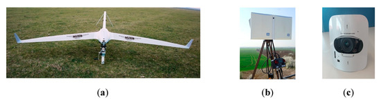
Figure 1.
System components: (a) UAV fixed wing; (b) ground terminal, and (c) payload photo.

Table 1.
UAV—characteristics and technical specifications.
A portion of the UAV, namely flight to image acquisition (GPS points marked), is presented in Figure 2a. From the successive images, acquired as the result of area surveillance, an orthophotoplan was created with special software (Figure 2b). To this end, the successive images overlapped in both length and width up to 60%. Then, images of 6000 × 4000 pixels were cropped and regions like flood and vegetation were segmented based on the following operations described in the above section: image decomposition in non-overlapped patches of dimension 64 × 64 pixels; patch classification and marking; and, finally, patch recombination. Some patches were difficult to be analyzed because of mixed zones. We created a database of 2000 images from flooded rural areas.
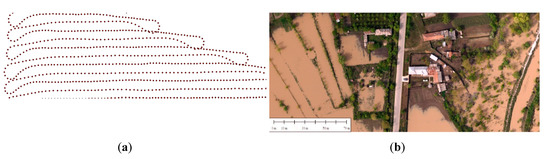
Figure 2.
Image acquisitions: (a) the UAV trajectory—photogrammetry (cropped); (b) the orthophotoplan (cropped).
3.2. YOLO Network
The CNN named decision YOLO, proposed in [39], operates at a global level, and the architecture is presented in Figure 3. The network has only convolutional layers grouped in two parts: down sampling and up sampling. The number of parameters in each dimension ascending layer is equal to the number of parameters in the correspondent layer on the descending side, establishing a connection between them.
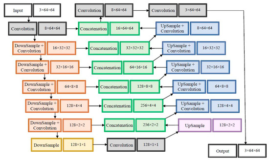
Figure 3.
Decision YOLO proposed architecture.
The proposed network was created starting from YOLO by applying five combinations of convolutional layers followed by max pooling (the down sampling stream) and then five combinations of convolutional layers followed by the up sampling. The architecture contains concatenations between the obtained ascending layer and the descending layer of the same dimensions (a U-net structure). For every two layers, the number of parameters doubles. Finally, the classification probability is provided, and this is used in the convolutional layer of the global classifier. In the integrated scheme of the proposed system, YOLO CNN is referred to as the primary classifier PC1. In the case of the YOLO network, it was observed that the size of the patch sometimes influences the decision of the network. In the case of the presented application, the chosen size was 64 × 64 pixels, taking into account the size of the UAV images. An essential quality of these networks is the short learning time.
3.3. GAN Network
In this work, a modified variant of the original GAN was used, namely conditional GAN (cGAN) [48], by considering, as starting images, a pair of an original image and an original mask of the segmented image [46]. The generator component (G) of cGAN is of the encoder–decoder, U-net type (Figure 4). This typical architecture successively down samples the data to a point and then applies the inverse procedure. Multiple connections between the encoder and decoder at corresponding levels can be observed at the G structure. The discriminator (D) role is to provide the information with an associated probability that a generated mask from G is a real one. Both G and D are based on typical layers, as presented in Table 2.
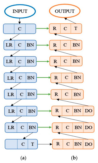
Figure 4.
The architecture of the generative adversarial network (GAN) generator: (a) the encoder; (b) the decoder. R—rectified linear unit, LR—leaky rectified linear unit, C—convolutional layer, BN—batch normalization, DO—dropout layer, and T—tanh function.
Table 2.
CNN layers description.
ReLU (R) is a function of activation of a neuron that implements the mathematical function (1):
In certain situations (Figure 4), it is preferable to consider the negative values and then use the LeakyReLU (LR) variant that lets the negative fraction of the input pass (2).
Like in the case of YOLO net, it should be noted that the use of the direct links in U-net [49] of the generator does not stop the normal flow of data. As seen in Figure 4, there are three dropouts (DOs).
The dropout level is the simplest way to combat the overfitting and involves the temporary elimination of some network units. DO is active only in the learning phase. The T unit that appears at the last level of G is the tanh function (3).
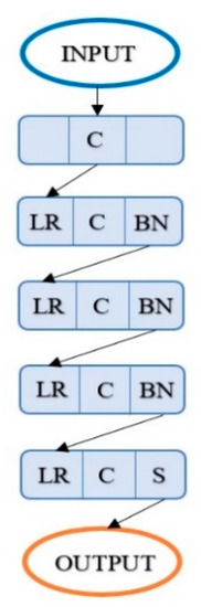
Figure 5.
The architecture of the GAN discriminator. LR—leaky rectified linear unit, C—convolutional layer, BN—batch normalization, and S—sigmoid function.
These two main components are connected in a complex architecture (Figure 6), inspired from [46], especially in the learning phase, where both G and D internal weights are established. As stated above, the architecture is a conditional generative adversarial network with the objective function V(D,G) (5).
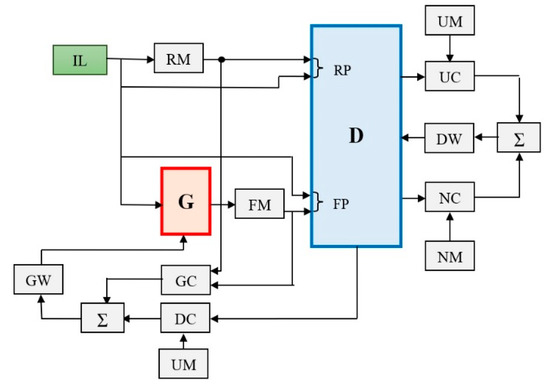
Figure 6.
Block diagram of the cGAN based system for flood and vegetation detection. The following notation were used: IL—image for learning; RM—real mask; G—generator; FM—fake mask; RP—real pair; FP—fake pair; D—discriminator; UM—unit matrix; UC—unit comparator; DW—weights for the discriminator; Σ—adder; NC—null comparator; NM—null matrix; GW—weights optimizer for the generator; DC—comparator for D with UM; GC—comparator for G between RM and FM.
In the learning phase, a set of patches are used to create the corresponding real masks (RM) of flood or vegetation. The same set is introduced in G to obtain fake masks (FM). Two image pairs, RP and FP (real and fake), are considered as D inputs [46]. There are four comparators (two for D and two for G) that are based on the binary cross entropy criterion for comparisons.
One goal is to minimize the error and gradient between the real segmented image and a unit matrix of 1 (UM). Another goal is to minimize the error and gradient between the fake segmented image and a null matrix of 0 (NM). The results are then used, via a weight optimizer (GW for G and DW for D), to update the weights. The procedure is repeated until the desired number of epochs (iterations) is reached.
G is effectively used only in the learning phase to establish the weights of D. Further, the role of D is to decide whether there is a real image or a fake image and, especially, to provide the decision probability. Due to sigmoid function (4), D provides a value between [0,1] that is the probability that a mask is a real one and this is the probability that the tested patch belongs to a class. cGAN is referred as primary classifier PC2 in the global classifier structure. The learning images (IL) come from our dataset with three classes: flood, vegetation, and rest.
The following technologies were used to test the GAN: Torch, a machine learning framework, to implement the neural network and Python (namely the NumPy, and PIL—Python Image Library—libraries), to evaluate the accuracy of cGAN results.
3.4. LENET
The LeNet-inspired network, containing five pairs of one convolutional layer followed by one max pooling layer, was created as in Figure 7 [39]. For simplicity, the number of parameters from one convolution to another was always doubled. In addition, the network contained one flattening layer and seven fully connected layers (dense). Although LeNet is considered effective in recognizing handwritten characters, and the modified alternative has been used successfully in segmenting regions of interest in aerial imagery [39]. In the experiments of the proposed application it was proved that it could intervene in a complementary way as a consensus agent of the global system.
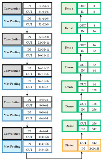
Figure 7.
LeNet architecture.
The cost function used is categorical cross-entropy (6), where N is the number of patches, C is the number of classes, is the prediction, and is the correct element that is considered as the probability that the patch i belongs to the class j. In the case of a decision, a patch is considered as belonging to the class with the highest probability. LeNet is considered as primary classifier PC3 in the proposed global system.
3.5. ALEXNET
AlexNet is considered as primary classifier PC4 in the proposed global system. It was chosen because it sometimes reacted complementarily to the other networks in the field of false positive or false negative areas, thereby contributing to the improvement of the overall classifier performance. The proposed AlexNet classifier, inspired from [33] is presented in Figure 8. This deep CNN has the ability of fast network training and the capability of reducing overfitting due to dropout layers.
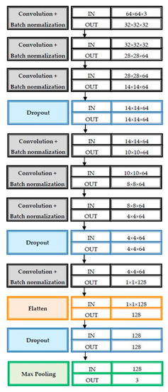
Figure 8.
AlexNet architecture.
The activation function, used at the output, was Softmax, which ensured the probability of the image (patch) being part of one of the three classes: F, V, and R. In order to increase the image number for the training phase we used the data augmentation by rotation (90°, 180°, 270°).
3.6. RESNET
ResNet is an ultra-deep feedforward network with residual connections, designed for large scale image processing. It can have different numbers of layers: 34, 50 (the most popular), 101 (our choice), etc. ResNet resolved the gradient vanishing problem and had a good position in image classification top-5 error.
The ResNet (residual net) architecture, used as primary NN classifier PC5, is presented in Figure 9. This deeper network has one of the best performances on object recognition accuracy. ResNet is composed from building blocks (modules), marked by A and B in Figure 9, with the same scheme of short (skip) connections. The shortcuts are used to keep the previous module outputs from possible inappropriate transformations. The blocks are named residual units [34] and are based on the residual function F (7), (8):
where is the block input, is the block output, is the set of weights associated with the n block, and f is ReLU.
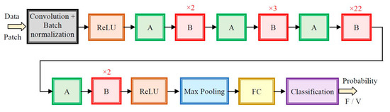
Figure 9.
ResNet architecture (A and B—repetitive modules described in Figure 10, FC—fully connected layer, F—flood type patch, V—vegetation type patch, and ×n—number of module repetition).
A pipeline of repetitive modules A and B is described in detail in Figure 10a and Figure 10b respectively.
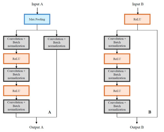
Figure 10.
Repetitive modules in ResNet configuration.
4. System Implementation
4.1. System Architecture
As previously mentioned, the proposed system contains five primary classifiers of the deep neural network type (PCi, i = 1,2,…,5), that have two contributions each: the weights (wi, i = 1, 2,…, 5), established in the validation phase, and the probabilities (pi, i = 1, 2,…, 5), provided at each classification/segmentation operation (operating phase).
A PC weight is expressed as its accuracy ACC (9) computed from parameters of confusion matrix (TP, TN, FP, and FN are true positive, true negative, false positive, and false negative cases, respectively):
A score Sj (j = F, V, R) is calculated for each class (F, V, and R) as can be seen in Equations (10), (11), and (12), respectively. These Equations are convolutional laws. The decision is made by the aid of a decision score (DS), and the class corresponds to the index obtained by maximum DS selection (13).
The main operating steps of the system are as follows and the flow chart is presented in Figure 11:
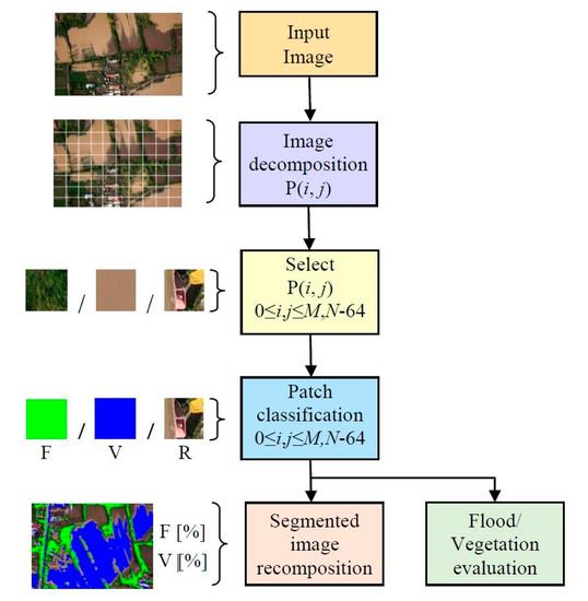
Figure 11.
Flow chart of the global system (F—flood class, V—vegetation class, and R—rest class).
1. The image is decomposed into patches of fixed size (64 × 64 pixels).
2. A patch is passed in parallel through neural networks to obtain individual classification probabilities.
3. The probabilities are merged by the convolutional law that characterizes the system, and the final decision of belonging to one of the classes F, V, R is taken.
4. The patch is marked according to the respective class.
5. The patch is reassembled into an image of the same size as the original image.
6. Return to step 2 until the patches in the original image are finished.
7. The segmented image results.
8. Additionally, the counting of patches from each class is done in order to evaluate the extent of the specific flood and vegetation areas.
The architecture of the proposed system, based on a decision fusion, expressed by the previous Equations (10)–(13) is presented in Figure 12. The system contains five classifiers, experimentally chosen, based on the individual accuracy evaluated for each classification task and detailed in the next section.
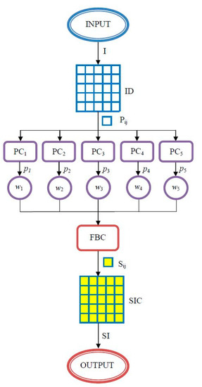
Figure 12.
Architecture of the image segmentation proposed system. I—input image, ID—image decomposition module, Pij—patch (i,j) as input, PCi—primary classifier i, pi—probability provided by PCi, wi the weight associated with PCi, FBC—fusion based classifier, Sij—patch (i,j) as output (segmented), SIC—segmented image recomposition module, and SI—segmented image.
The meanings of the notations in Figure 12 are the following: I—image to be segmented (input), ID—image decomposition in patches, Pi,j—patch of I on (i,j) position, PCk—primary classifier (PC1—YOLO, PC2—GAN, PC3—LeNet, PC4—AlexNet, and PC5—ResNet), pk—probability of Pi,j classification by PCk, wk—weight according to primary classifier PCk, FBC—fusion based classifier, which indicates the patch class and provides the marked patch, Si,j—patch classified, SIC—segmented image re-composition from classified patches, and SI—segmented image (output).
As can be seen from the previous Equations and Figure 12, a new convolutional layer is made by the FBC module with the weights wi, (fixed after validation phase). The inputs are the probabilities pi, , provided by the primary classifiers, and the output is the decision based on Equations (10)–(13).
The execution time differs from a network to network and of the system implementation. A reduced time was obtained on GPU (graphics processing unit) implementation. The execution time for learning was about 15 h, and the time for segmentation was about 0.2 s for an image. The system architecture used for experimental results consisted of the following: Intel Core I7 CPU, 4th generation, 16 GB RAM, NVIDIA GeForce 770 M (Kepler architecture), 2 GB VRAM, Windows 10 operating system, Microsoft Visual Studio 2013.
4.2. System Tuning: Learning, Validation, and Weight Detection
For the application envisaged in the paper, the system used three phases: learning, validation, and testing (actual operation). First, the learning phase was separately performed for each primary classifier, directly or by transfer learning, to obtain the best performances in terms of time and accuracy. Next, in a similar manner, in the validation phase the attached weight was obtained for each classifier. Finally, the images were processed by the global system presented in Figure 12.
From the images cropped from orthophotoplan, 4500 patches were selected for learning (1500 flood patches, 1500 vegetation, and 1500 from the rest). Similarly, 1500 patches were selected for validation (500 from each class). As mentioned above, the weight associated with the primary classifiers were established in the validation stage. Examples of such patches are presented in Figure 13.

Figure 13.
Examples of patches for flood (F), vegetation (V), and rest (R) for learning phase (our dataset).
For simplicity, we considered that the patches selected for training and validation contained pixels from a single type of region (F, V, or R). Since the convolution operation is not independent of changes of rotation and mirroring, they could be applied to simulate new cases for the network. Thus, on the patches obtained previously, a 90° rotation was applied, and then a mirror was used to increase the image number four times (18,000 for learning and 6000 for validation). Both learning and validation were performed separately for the three types of regions (F, V, or R). Examples of flood and vegetation segmentation based on YOLO (PC1), GAN (PC2), LeNet (PC3), AlexNet (PC4), and ResNet (PC5) are given in Figure 14 (our dataset). For comparison, the original image and manual segmentation versus predicted segmentation images are presented. As can be seen, errors of segmentation were presented at the edges because of the mixed regions.
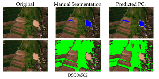
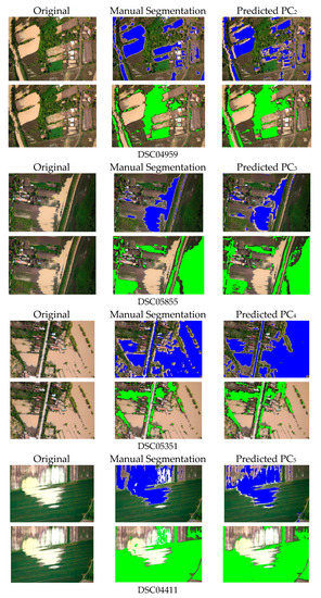
Figure 14.
Flood and vegetation segmentation (manual and predicted) for individual classifiers (validation phase)—our dataset.
For each of the five neural networks and of the three classes, the confusion matrices were calculated (examples in Figure 15 are given for YOLO, F, and V classes). Based on the confusion matrices, the performance parameters TP, TN, FP, FN, and ACC from (9) were evaluated. ACC for flood (92.8%) was better than the ACC for vegetation (87.5%), because, generally, a flood patch is more uniform than a vegetation patch. As a result, the weights (Table 3) were evaluated (by two digit approximation) for the primary classifiers PC1, PC2, PC3, PC4, and PC5, and, also, for each RoI (F, V, and R). To this end the table presents the intermediate parameters (TP, TN, FP, and FN) to calculate ACC and, finally, the weights. All the parameters were indexed by the class label (F, V, and R). It can be seen the accuracy was dependent on PCs and classes. Thus, the flood accuracy ACC-F was greater than other accuracies (ACC-V, vegetation, and ACC-R, rest) for all classifiers due to the reason mentioned above.
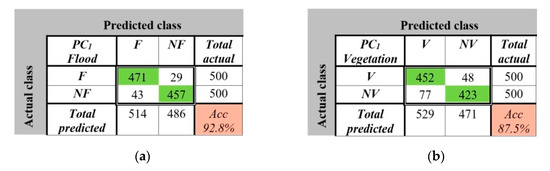
Figure 15.
Confusion matrices for flood (a) and vegetation (b) detection in the case of primary classifier PC1.
Table 3.
Associated weights for the primary classifiers (PC).
The meaning of the notations in Table 3 is as follows: NN-the neural network used, TP, TN, FP and FN are the true positive cases, true negative, false positive and false negative, respectively, ACC-accuracy, w-associated weight. They are associated with classes: F-flood, V-vegetation and R-rest. Thus, TP-F means the true positive in terms of flood detection, ACC-accuracy in flood detection, wF-weight for flood detection, etc.
5. Experimental Results
After learning and validation of the individual classifiers, the proposed system was tested in a real environment. Like in the previous phases, the images were obtained from a photogrammetry flight over the same rural area in Romania after a moderate flood in order to accurately evaluate the damages in agriculture. Thus, our own dataset was obtained.
In the operational phase, the RoI segmentation was performed by the global system proposed in Figure 12. First, the image extracted from the orthophotoplan was decomposed in patches according to the methodology described in Section 3. The patch classification and segmentation were performed based on Equations (10–13), with the weights obtained in the validation phase (Table 3). For each patch, a primary classifier (Figure 12) gives the probability to belong to a predicted class (see pij from Table 4). Some examples of patch classification and segmentation are given in Table 4. The decision score S is calculated as in Equation (13). The resulted patches are colored with blue (F), green (V), or are maintained as the initial (R). The real patches and the segmented patches are labeled by the class name. For correct segmentation, in Table 4 on the same raw, the original and segmented images pair has the same label (F-F; V-V, or R-R). As can be seen, in the last row of Table 4, there is a false segmentation decision (R-F).
Table 4.
Examples of patch classification results.
The decision score is also approximated by three digits. In this operational phase, the primary classifiers provide only the probabilities as the evaluated patch belongs to a predicted class and the fusion based classifier evaluates the decision score for the final classification. After image re-composition, the segmented images are shown as in Figure 16. The examples in Table 4 show that most patches were correctly classified by all PCs except the last two. The penultimate patch was misclassified by four PCs and the overall result was a misclassification. The last patch was misclassified by two classifiers (PC1 and PC4), but the global classifier result was correct.
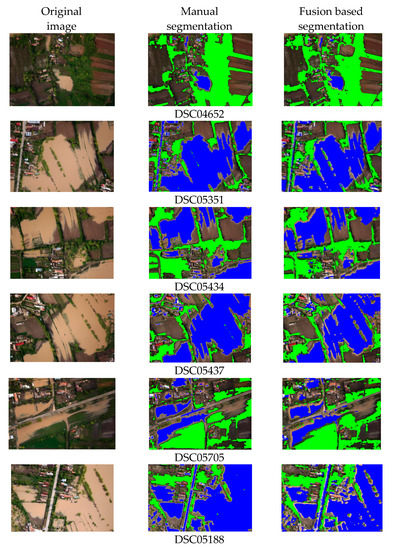
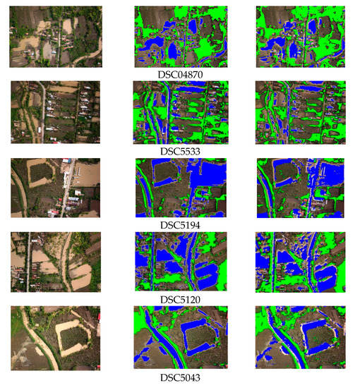
Figure 16.
Examples of flood and vegetation segmentation by fusion-based classifier (testing phase)—our dataset.
In order to evaluate the flood extension and the remaining vegetation, from each analyzed image, the percentage of flood area (FA) and vegetation area (VA) were calculated in manual (MS) and automatic (AS) segmentation cases (Table 5). Finally, the percentage occupancy of flood and vegetation, from the total investigated area, was evaluated as the average of image occupancy (the last row—Total—in Table 5). It can see that, generally, the flood segmentation was more accurate than the vegetation segmentation. Compared with the manual segmentation, the flood evaluation differed by 0.53%, and the vegetation evaluation differed by 0.84%.
Table 5.
Percentage of the whole image area occupied by each RoI (FA—flooded area, VA—vegetation area, MS—manual segmentation, AS—automatic segmentation).
6. Discussion
The proposed system based on decision fusion combines two sets of information: the PC weights obtained in a distinct validation phase, and the probabilities obtained in the testing (operational) phase. The primary neural networks were first experimentally tested. Accuracy differs from one network to another and from one type of class to another. Thus, in Table 6 are presented the accuracies of individual networks (YOLO, GAN, LeNet, AlexNet, and ResNet) and of the global system for each class (F, V, and R) and the mean. It can be observed that for individual networks, the best results were obtained for ResNet and flood.
Table 6.
Accuracy comparison with primary classifiers.
In case of the experiments described in this paper, the accuracy was lower for the YOLO network, for the patch size of 64 × 64 pixels (86.7%). The authors analyzed the performance of the YOLO network on different patch sizes for the same images and found the following: for the 128 × 128 pixel size of the patch, the accuracy was 89% [39], and for 256 × 256 pixel size the accuracy was 91.2%. This is explained by the mechanism of network operation within the convolution to preserve the size of the patch. The proposed system is adaptable for different patch sizes. In cases of more extensive floods, where no small portions of water mixed with vegetation appear, the system operates with larger patch sizes, and the YOLO network will have a better accuracy (respectively, a higher weight in the global decision).
On the other hand, the purpose of combining several networks was to reduce the individual number of false positive and false negative decisions. It was found that in some cases the decision of the YOLO network leads to a global correct decision. This aspect is also a motivation for choosing several neural networks for the global classification system.
Although the fusion based on a majority vote would have been simpler, we chose a fusion decision that takes into account a more complex criterion based on two elements: a) the "subjectivism" of each network, expressed by the probability of classification, and b) the rigid weights of these networks, previously established (in the validation phase). This is the new convolutional layer of the proposed system that leads to a more objective classification criterion than a simple vote criterion.
Why five networks and not more or less remains an open question. It is a matter of compromise, assumed by our experimental choice. A large number would lead to greater complexity, so a greater computational effort and time, while a small number would lead to lower accuracy.
The classification results were good (Table 6); however, due to images that were difficult to interpret, erroneous results were also obtained. The main difficulties consist of factors such as (a) the parts of the ground that were wet or recently dried were possibly confused with flood (error R-F), (b) the vegetation that was uneven was possibly confused with class R (V-R error), and c) possible green areas (trees) covered the flooded area (V-F error), etc. One such example is presented in Table 4, the last row; this is because it contains a surface of land, recently dried, similar with the flood (error R-F).
The obtained results were better than the individual neural networks (Table 6) and better or similar than other works (Table 7).
Table 7.
Accuracy comparison with other works.
The papers in Table 7 were mentioned in the Introduction or Related Work sections and refer to similar works as ours. Only paper [39] addressed both flood and vegetation classification. The results obtained with different deep CNNs have less accuracy than our global system. The authors in [1] used UAV images for vegetation segmentation, particularly different crops, based on hue color channel and corresponding histogram with different thresholds. The methods in Table 7 were tested on our database for papers [29] and [39]. In [1] the images are very similar to ours. The images in [4] and [13] are very different from our application (urban).
The authors in [4] used a VGG-based fully convolutional network (FCN-16s) for flooded area extraction from UAV images on a new dataset. However, our data set is more complex and difficult to segmentation. Compared with traditional classifiers such as SVMs, the obtained results are more accurate. As in our study, the problem of floods hidden under trees remains unresolved.
Our previous work [25] combines an LBP histogram with a CNN for flood segmentation, but the results are less accurate and the operating time is longer because for each patch the LBP histogram must be calculated.
The images that characterize the two main classes, flood and vegetation, may differ inside an orthophotoplan due to the characteristics of the soil (color and composition) that influence the flood color or the texture and color of the vegetation. There are also different features for different orthophotoplans depending on the season and location. Obviously, for larger areas there is the possibility of decreasing accuracy. We recommend a learning action at each application from as many different representative patches as possible.
The network learning was done from patches considered approximately uniform (containing only flood or vegetation). Due to this reason, a smaller segmented area was usually obtained (mixed areas being uncertain). Other characteristic areas, such as buildings and roads, are less common in agricultural regions. They were introduced to the "rest" class. Another study [46] found that the roads (especially asphalted) cannot be confused with floods.
Compared to our previous works, [29] and [39], this paper introduces several neural networks, selected after performance analysis, in an integrative system (the global system) based on fusion of decisions (probabilities). This system can be considered as a network of convolutional networks, the unification layer being also based on a convolution law (10–12).
One of the weak points of our approach is the empirical choice of the neural networks that make up the global system (only based on experimental results). We have relied on our experience in recent years and on the literature. On the other hand, we have modified the well-known networks in order to obtain the best possible performances for our own database. The images used were very difficult to interpret because they contain areas at the boundary between flood and non-flood (for example, wetland and flood), and areas of vegetation are not uniform. On clearly differentiable regions of interest, the results are much better, but we wanted to demonstrate the effectiveness on real, difficult cases.
Neural image processing networks are constantly evolving, modernizing the old ones and appearing new ones. In this case, the question arises: how many and why are the networks involved in such a fusion based system? It is desired to develop a mathematical criterion, an objective, based on optimizing parameters such as time, processing cost, accuracy, etc., to take into account the specific application.
7. Conclusions
In this paper, we proposed an efficient solution for segmentation and evaluation of the flood and vegetation RoIs from aerial images. The system proposed combines in a new convolutional layer the outputs of five classifiers based on neural networks. The convolution is based on weights and probabilities and improves the accuracy of classification. This fusion of neural networks into a global classifier has the advantage of increasing the efficiency of segmentation demonstrated by the examples presented. Images tested and compared were from own database acquired with a UAV in a rural zone. Compared to other methods presented in the references, the accuracy of the method proposed increased for both flood and vegetation zones.
As feature work, we proposed the segmentation of more RoIs from UAV images using multispectral cameras. For more flexibility and adaptability to illumination and weather conditions we will also consider the radiometric calibration of images. We also want to create a bank of pre-trained neural networks that can be accessed and interconnected, depending on the application, to obtain the most efficient fusion classification system.
We want to expand the application for monitoring the evolution of vegetation, which means both the creation of vegetation patterns and the permanent adaptation to color and texture changes that take place during the year.
Author Contributions
L.I. contributed to the conception and design of the CNN, performed the experiments, and edited the paper. D.P. conceived of the paper, contributed to processing the data, analyzed the results, and selected the references. All authors have read and agreed to the published version of the manuscript.
Funding
This research was funding by University POLITEHNICA of Bucharest.
Acknowledgments
The work was supported by University POLITEHNICA of Bucharest, and project NETIO, subsidiary MUWI, 1224/ 2018.
Conflicts of Interest
The authors declare no conflict of interest.
References
- Hassanein, M.; Lari, Z.; El-Sheimy, N. A New Vegetation Segmentation Approach for Cropped Fields Based on Threshold Detection from Hue Histograms. Sensors 2018, 18, 1253. [Google Scholar] [CrossRef] [PubMed]
- Mavridou, E.; Vrochidou, E.; Papakostas, G.; Pachidis, T.; Kaburlasos, V. Machine Vision Systems in Precision Agriculture for Crop Farming. J. Imaging 2019, 5, 89. [Google Scholar] [CrossRef]
- Popescu, D.; Ichim, L.; Caramihale, T. Flood areas detection based on UAV surveillance system. In Proceedings of the 2015 19th International Conference on System Theory, Control and Computing (ICSTCC), Cheile Gradistei, Romania, 14–16 October 2015; Institute of Electrical and Electronics Engineers (IEEE): Piscataway, NJ, USA, 2015; pp. 753–758. [Google Scholar]
- Gebrehiwot, A.; Hashemi-Beni, L.; Thompson, G.; Kordjamshidi, P.; Langan, T.E. Deep Convolutional Neural Network for Flood Extent Mapping Using Unmanned Aerial Vehicles Data. Sensors 2019, 19, 1486. [Google Scholar] [CrossRef] [PubMed]
- Panboonyuen, T.; Jitkajornwanich, K.; Lawawirojwong, S.; Srestasathiern, P.; Vateekul, P. Road Segmentation of Remotely-Sensed Images Using Deep Convolutional Neural Networks with Landscape Metrics and Conditional Random Fields. Remote. Sens. 2017, 9, 680. [Google Scholar] [CrossRef]
- Li, Y.; Peng, B.; He, L.; Fan, K.; Tong, L. Road Segmentation of Unmanned Aerial Vehicle Remote Sensing Images Using Adversarial Network With Multiscale Context Aggregation. IEEE J. Sel. Top. Appl. Earth Obs. Remote. Sens. 2019, 12, 2279–2287. [Google Scholar] [CrossRef]
- Shen, S.; Cheng, C.; Yang, J.; Yang, S. Visualized analysis of developing trends and hot topics in natural disaster research. PLoS ONE 2018, 13, e0191250. [Google Scholar] [CrossRef]
- Scott-Smith, T. Paradoxes of Resilience: A Review of the World Disasters Report 2016. Dev. Chang. 2018, 49, 662–677. [Google Scholar] [CrossRef]
- Helber, P.; Bischke, B.; Dengel, A.; Borth, D. Introducing Eurosat: A Novel Dataset and Deep Learning Benchmark for Land Use and Land Cover Classification. In Proceedings of the IGARSS 2018—2018 IEEE International Geoscience and Remote Sensing Symposium, Valencia, Spain, 22–27 July 2018; pp. 204–207. [Google Scholar] [CrossRef]
- Libelium World, Early Flood Detection and Warning System in Argentina Developed with Sensors Technology, Case Studies, Meshlium, Plug & Sense!, Smart Cities, Smart Water, Waspmote, 2018. Available online: http://www.libelium.com/early-flood-detection-and-warning-system-in-argentina-developed-with-libelium-sensors-technology/ (accessed on 23 March 2020).
- Gomez, C.; Purdie, H. UAV-based Photogrammetry and Geocomputing for Hazards and Disaster Risk Monitoring—A Review. Geoenviron. Disasters 2016, 3, 496. [Google Scholar] [CrossRef]
- Li, Y.; Tao, C.; Tan, Y.; Shang, K.; Tian, J. Unsupervised Multilayer Feature Learning for Satellite Image Scene Classification. IEEE Geosci. Remote Sens. Lett. 2016, 13, 157–161. [Google Scholar] [CrossRef]
- Feng, Q.; Liu, J.; Gong, J. Urban Flood Mapping Based on Unmanned Aerial Vehicle Remote Sensing and Random Forest Classifier—A Case of Yuyao, China. Water 2015, 7, 1437–1455. [Google Scholar] [CrossRef]
- Arif, M.S.M.; Gülch, E.; Tuhtan, J.A.; Thumser, P.; Haas, C. An investigation of image processing techniques for substrate classification based on dominant grain size using RGB images from UAV. Int. J. Remote. Sens. 2016, 38, 2639–2661. [Google Scholar] [CrossRef]
- Milas, A.S.; Arend, K.; Mayer, C.; Simonson, M.A.; Mackey, S. Different colours of shadows: Classification of UAV images. Int. J. Remote Sens. 2017, 38, 3084–3100. [Google Scholar] [CrossRef]
- Lo, S.-W.; Wu, J.-H.; Lin, F.-P.; Hsu, C.-H. Cyber Surveillance for Flood Disasters. Sensors 2015, 15, 2369–2387. [Google Scholar] [CrossRef] [PubMed]
- Nazir, F.; Riaz, M.M.; Ghafoor, A.; Arif, F. Flood Detection/Monitoring Using Adjustable Histogram Equalization Technique. Sci. World J. 2014, 2014, 1–7. [Google Scholar] [CrossRef] [PubMed]
- Lo, S.W.; Wu, J.H.; Chen, L.C.; Tseng, C.H.; Lin, F.P. Flood Tracking in Severe Weather. In Proceedings of the 2014 International Symposium on Computer, Consumer and Control, Taichung City, Taiwan, 10–12 June 2014; pp. 27–30. [Google Scholar] [CrossRef]
- Rudner, T.G.J.; Rußwurm, M.; Fil, J.; Pelich, R.; Bischke, B.; Kopackova, V.; Bilinski, P. Multi3Net: Segmenting Flooded Buildings via Fusion of Multiresolution, Multisensor, and Multitemporal Satellite Imagery. In Proceedings of the AAAI Conference on Artificial Intelligence, 2019, Honolulu, HI, USA, 27 January–1 February 2019; Volume 33, pp. 702–709. [Google Scholar]
- Zhang, F.; Zhou, G. Estimation of vegetation water content using hyperspectral vegetation indices: A comparison of crop water indicators in response to water stress treatments for summer maize. BMC Ecol. 2019, 19, 18. [Google Scholar] [CrossRef]
- Smigaj, M.; Gaulton, R.; Suarez, J.D.; Barr, S. Use of Miniature Thermal Cameras for Detection of Physiological Stress in Conifers. Remote Sens. 2017, 9, 957. [Google Scholar] [CrossRef]
- Vidhya, K.; Revathi, S.; Sahaya Selva Ashwini, S.; Vanitha, S. Review on digital image segmentation techniques. Int. Res. J. Eng. Technol. 2016, 3, 618–619. [Google Scholar]
- Popescu, D.; Ichim, L.; Gornea, D.; Stoican, F. Complex Image Processing Using Correlated Color Information. Intell. Tutoring Syst. 2016, 10016, 723–734. [Google Scholar] [CrossRef]
- Popescu, D.; Ichim, L.; Stoican, F. Unmanned Aerial Vehicle Systems for Remote Estimation of Flooded Areas Based on Complex Image Processing. Sensors 2017, 17, 446. [Google Scholar] [CrossRef]
- Sumalan, A.L.; Popescu, D.; Ichim, L. Flooded and vegetation areas detection from UAV images using multiple descriptors. In Proceedings of the 2017 21st International Conference on System Theory, Control and Computing (ICSTCC); Institute of Electrical and Electronics Engineers (IEEE): Piscataway, NJ, USA, 2017; pp. 447–452. [Google Scholar]
- Kalantar, B.; Mansor, S.; Sameen, M.; Pradhan, B.; Shafri, H.Z.M. Drone-based land-cover mapping using a fuzzy unordered rule induction algorithm integrated into object-based image analysis. Int. J. Remote Sens. 2017, 38, 2535–2556. [Google Scholar] [CrossRef]
- Cao, X.; Zhou, F.; Xu, L.; Meng, D.; Xu, Z.; Paisley, J. Hyperspectral Image Classification With Markov Random Fields and a Convolutional Neural Network. IEEE Trans. Image Process. 2018, 27, 2354–2367. [Google Scholar] [CrossRef] [PubMed]
- Shi, C.; Pun, C.-M. Superpixel-based 3D deep neural networks for hyperspectral image classification. Pattern Recognit. 2018, 74, 600–616. [Google Scholar] [CrossRef]
- Cirneanu, A.L.; Popescu, D.; Ichim, L. CNN based on LBP for Evaluating Natural Disasters. In Proceedings of the 2018 15th International Conference on Control, Automation, Robotics and Vision (ICARCV), Singapore, 18–21 November 2018; Institute of Electrical and Electronics Engineers (IEEE): Piscataway, NJ, USA, 2018; pp. 568–573. [Google Scholar]
- Ju, C.; Bibaut, A.; Van Der Laan, M. The relative performance of ensemble methods with deep convolutional neural networks for image classification. J. Appl. Stat. 2018, 45, 2800–2818. [Google Scholar] [CrossRef] [PubMed]
- Minaee, S.; Boykov, Y.; Porikli, F.; Plaza, A.; Kehtarnavaz, N.; Terzopoulos, D. Image Segmentation Using Deep Learning: A Survey. arXiv preprint 2020, arXiv:2001.05566. [Google Scholar]
- LeCun, Y.; Bottou, L.; Bengio, Y.; Haffner, P. Gradient-based learning applied to document recognition. Proc. IEEE 1998, 86, 2278–2324. [Google Scholar] [CrossRef]
- Krizhevsky, A.; Sutskever, I.; Hinton, G.E. Pdf ImageNet classification with deep convolutional neural networks. Commun. ACM 2017, 60, 84–90. [Google Scholar] [CrossRef]
- He, K.; Zhang, X.; Ren, S.; Sun, J. Identity Mappings in Deep Residual Networks. Comput. Sci. ndash ICCS 2020 2016, 9908, 630–645. [Google Scholar] [CrossRef]
- He, K.; Zhang, X.; Ren, S.; Sun, J. Deep Residual Learning for Image Recognition. In Proceedings of the 2016 IEEE Conference on Computer Vision and Pattern Recognition (CVPR); Institute of Electrical and Electronics Engineers (IEEE): Piscataway, NJ, USA, 2016; pp. 770–778. [Google Scholar]
- Long, J.; Shelhamer, E.; Darrell, T. Fully convolutional networks for semantic segmentation. In Proceedings of the 2015 IEEE Conference on Computer Vision and Pattern Recognition (CVPR); Institute of Electrical and Electronics Engineers (IEEE): Piscataway, NJ, USA, 2015; pp. 3431–3440. [Google Scholar]
- Pang, S.; Ding, T.; Qiao, S.; Meng, F.; Wang, S.; Li, P.; Wang, X. A novel YOLOv3-arch model for identifying cholelithiasis and classifying gallstones on CT images. PLoS ONE 2019, 14, e0217647. [Google Scholar] [CrossRef]
- Artamonov, N.S.; Yakimov, P.Y. Towards Real-Time Traffic Sign Recognition via YOLO on a Mobile GPU. J. Phy. Conf. Ser. 2018, 1096, 012086. [Google Scholar] [CrossRef]
- Popescu, D.; Ichim, L.; Cioroiu, G. Deep CNN Based System for Detection and Evaluation of RoIs in Flooded Areas. Lect. Notes Comput. Sci. 2019, 11953, 236–248. [Google Scholar] [CrossRef]
- Redmon, J.; Divvala, S.; Girshick, R.; Farhadi, A. You Only Look Once: Unified, Real-Time Object Detection. In Proceedings of the 2016 IEEE Conference on Computer Vision and Pattern Recognition (CVPR), Las Vegas, NV, USA, 27–30 June 2016; Institute of Electrical and Electronics Engineers (IEEE): Piscataway, NJ, USA, 2016; pp. 779–788. [Google Scholar]
- Alom, Z.; Taha, T.M.; Yakopcic, C.; Westberg, S.; Sagan, V.; Nasrin, M.S.; Hasan, M.; Van Essen, B.C.; Awwal, A.A.S.; Asari, V.K. A State-of-the-Art Survey on Deep Learning Theory and Architectures. Electronics 2019, 8, 292. [Google Scholar] [CrossRef]
- Goodfellow, I.J.; Pouget-Abadie, J.; Mirza, M.; Xu, B.; Warde-Farley, D.; Ozair, S.; Courville, A.; Bengio, Y. Generative adversarial nets. In Proceedings of the International Conference on Neural Information Processing Systems (NIPS), Montreal, QC, Canada, 8–13 December 2014; pp. 2672–2680. [Google Scholar]
- Ali-Gombe, A.; Elyan, E.; Savoye, Y.; Jane, C. Few-shot Classifier GAN. In Proceedings of the 2018 International Joint Conference on Neural Networks (IJCNN), Rio de Janeiro, Brazil, 8–13 July 2018; Institute of Electrical and Electronics Engineers (IEEE): Piscataway, NJ, USA, 2018; pp. 1–8. [Google Scholar]
- Gong, M.; Xu, Y.; Li, C.; Zhang, K.; Batmanghelich, K. Twin Auxiliary Classifiers GAN. Adv. Neural Inf. Process Syst. 2019, 32, 1328–1337. [Google Scholar] [PubMed]
- Hwang, U.; Jung, D.; Yoon, S. HexaGAN: Generative Adversarial Nets for Real World Classification. In Proceedings of the 36th International Conference on Machine Learning, Long Beach, CA, USA, 9–15 June 2019; Volume 97, pp. 2921–2930. [Google Scholar]
- Popescu, D.; Ichim, L.; Docea, A. Complex Conditional Generative Adversarial Nets for Multiple Objectives Detection in Aerial Images. Lect. Notes Comput. Sci. 2018, 11304, 671–683. [Google Scholar] [CrossRef]
- EUROPA, Multisensory Robotic System for Aerial Monitoring of Critical Infrastructure Systems. Available online: https://trimis.ec.europa.eu/ (accessed on 9 April 2020).
- Mirza, M.; Osindero, S. Conditional Generative Adversarial Nets. arXiv preprint 2014, arXiv:1411.1784. [Google Scholar]
- Ronneberger, O.; Fischer, P.; Brox, T. U-Net: Convolutional Networks for Biomedical Image Segmentation. Lect. Note Comp. Sci. 2015, 9351, 234–241. [Google Scholar] [CrossRef]


© 2020 by the authors. Licensee MDPI, Basel, Switzerland. This article is an open access article distributed under the terms and conditions of the Creative Commons Attribution (CC BY) license (http://creativecommons.org/licenses/by/4.0/).