Greening and Browning Trends across Peru’s Diverse Environments


Abstract
1. Introduction
2. Materials and Methods
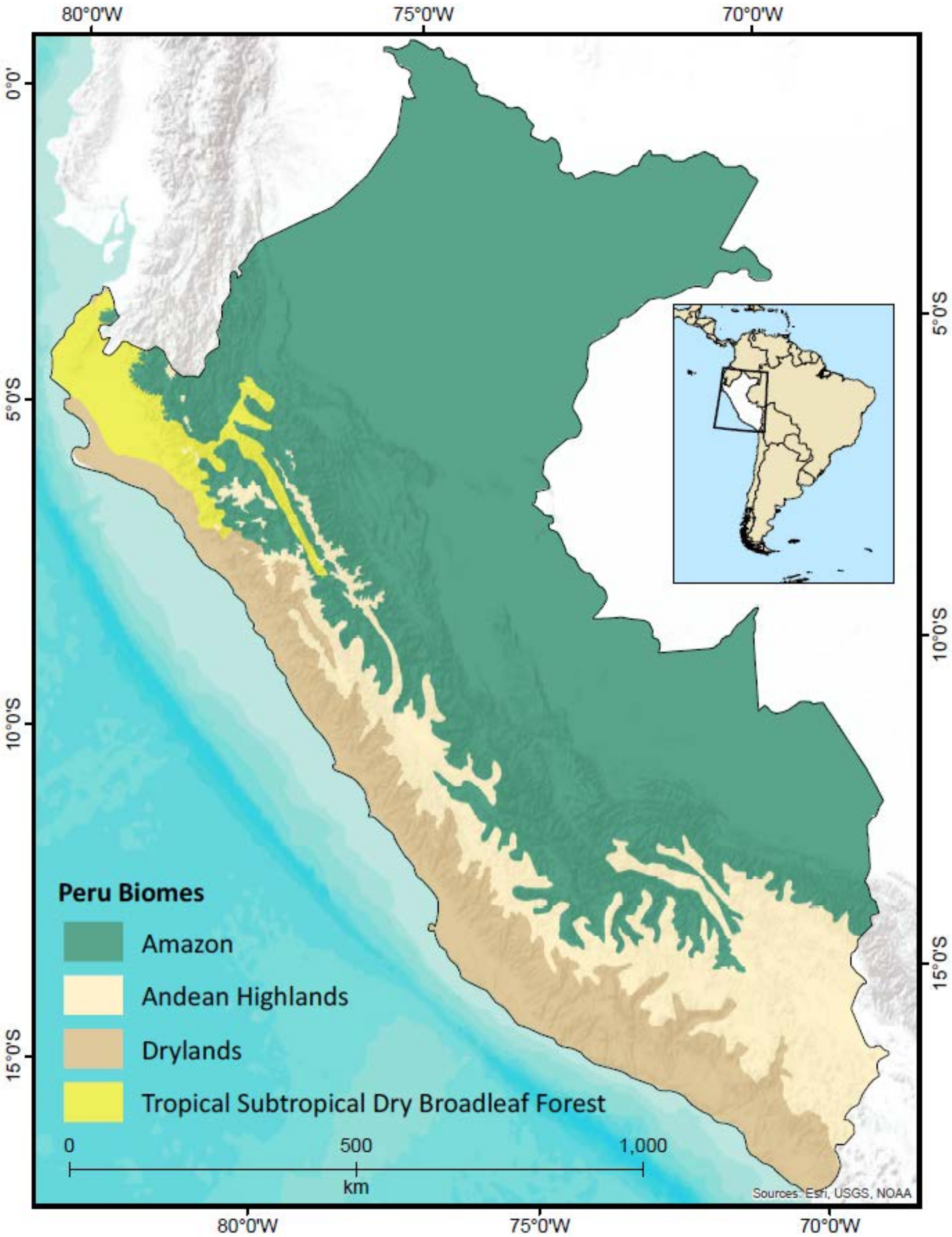
2.1. Study Area
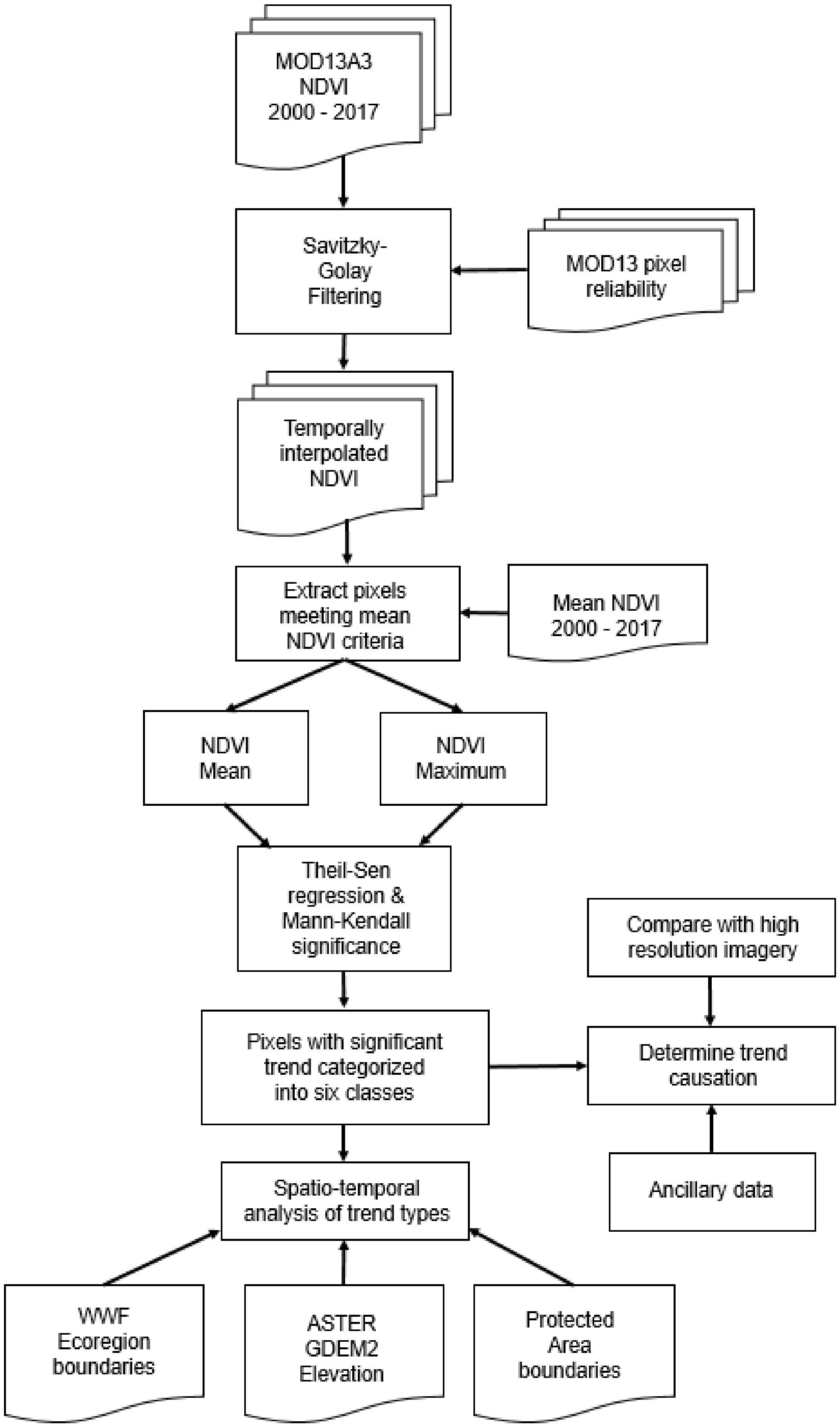
2.2. Remote Sensing Pre-Processing
2.3. MODIS Normalized Difference Vegetation Index Trend Analysis
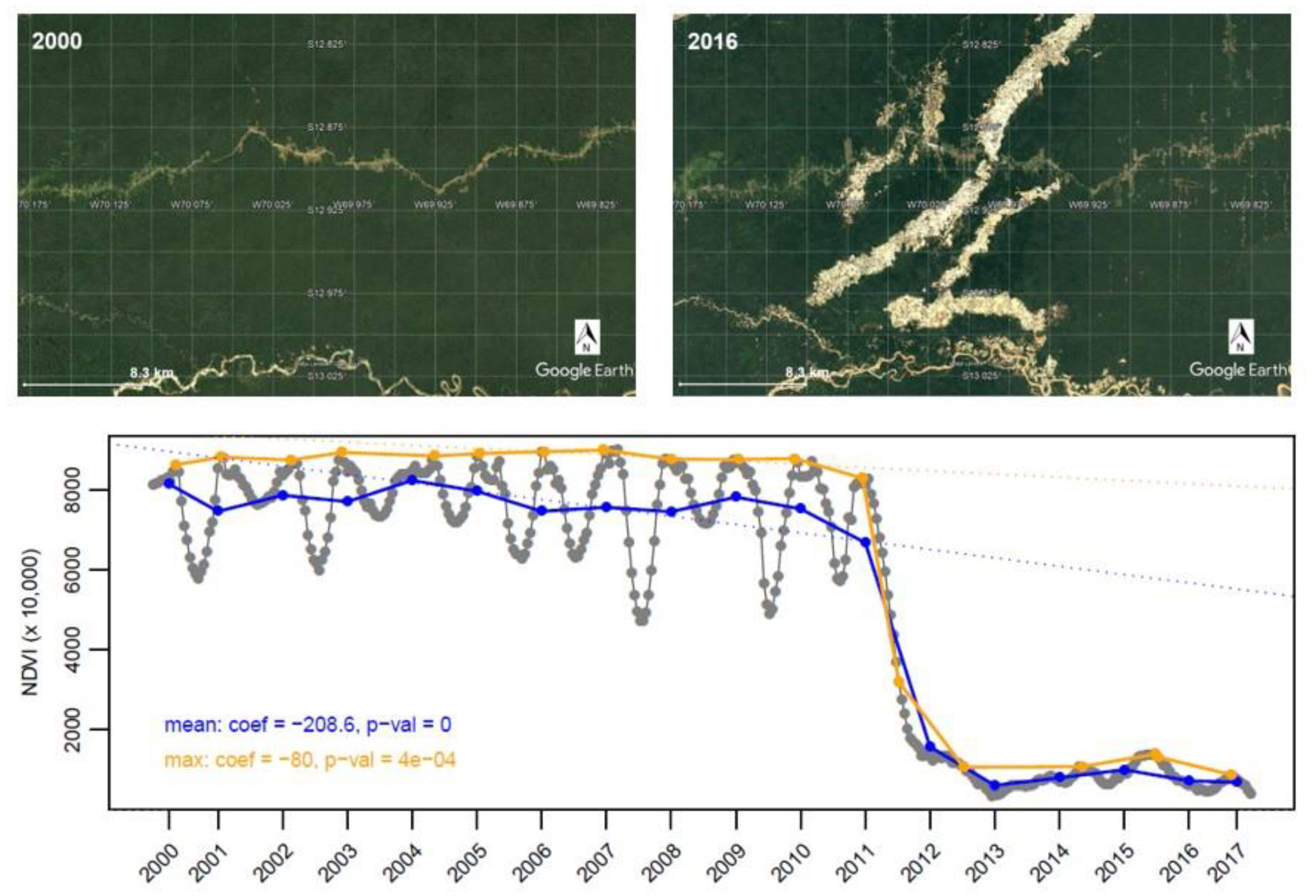
2.4. Exploring Causality
3. Results
3.1. Peru Overall
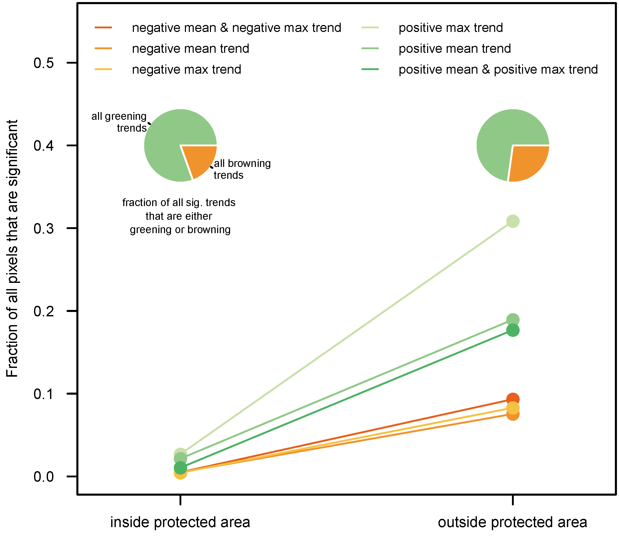
3.2. By Protected Area Status
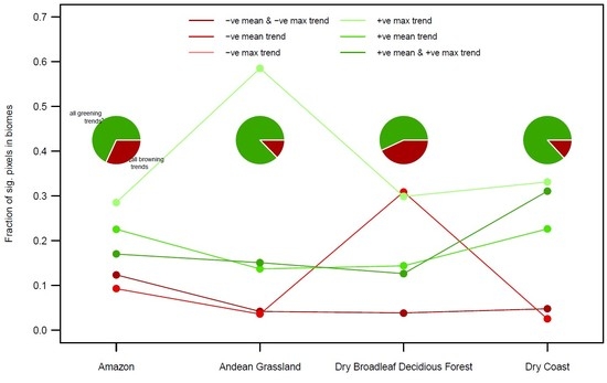
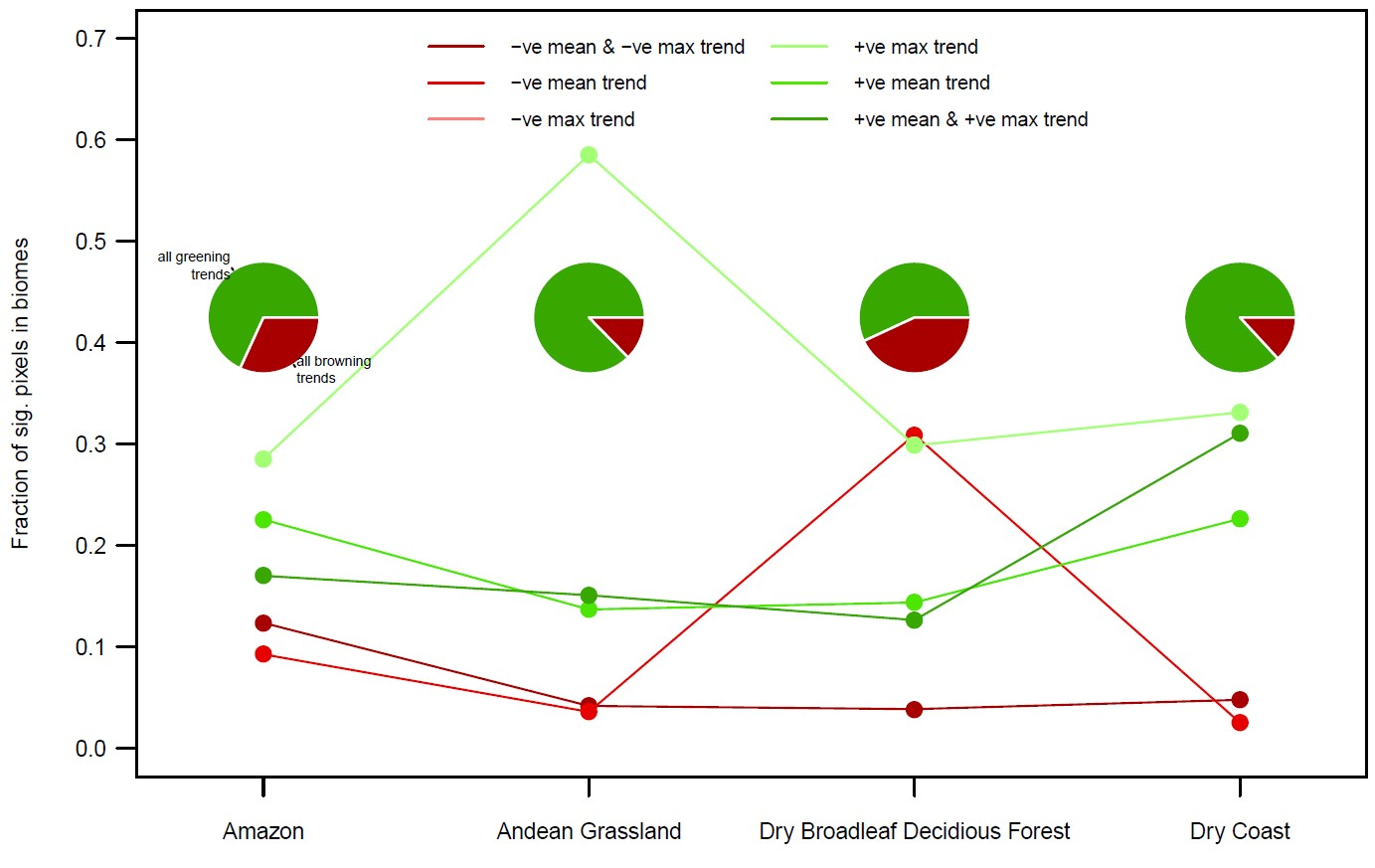
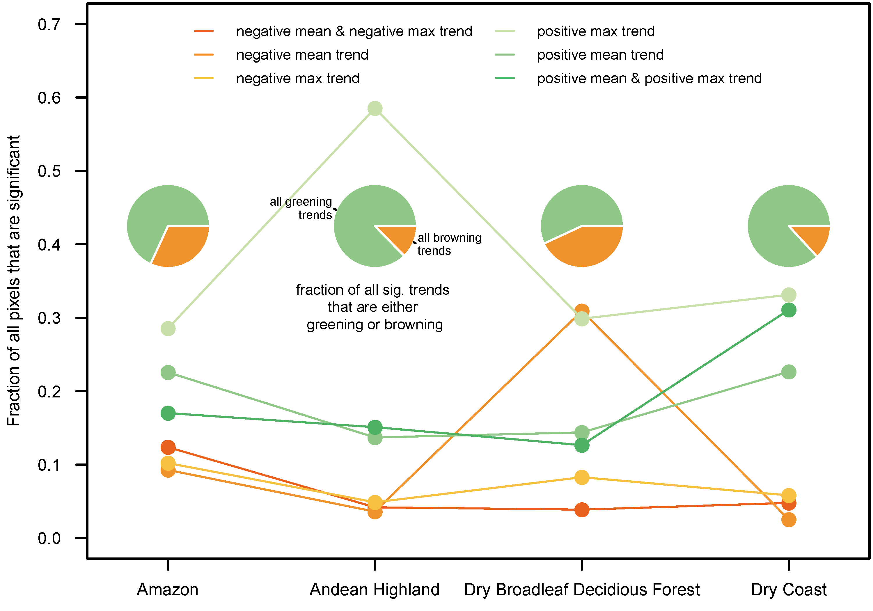
3.3. By Biome
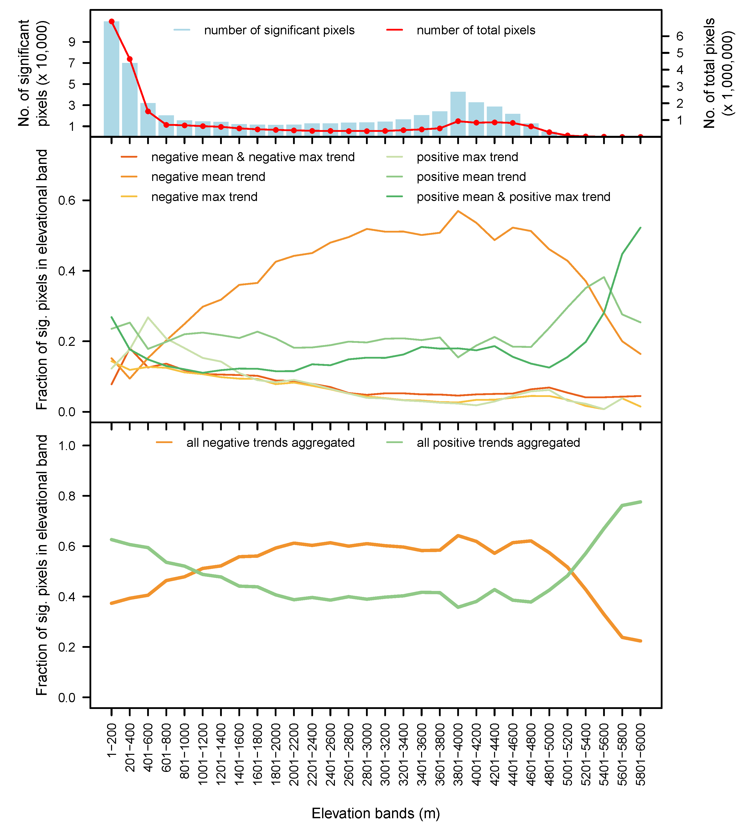
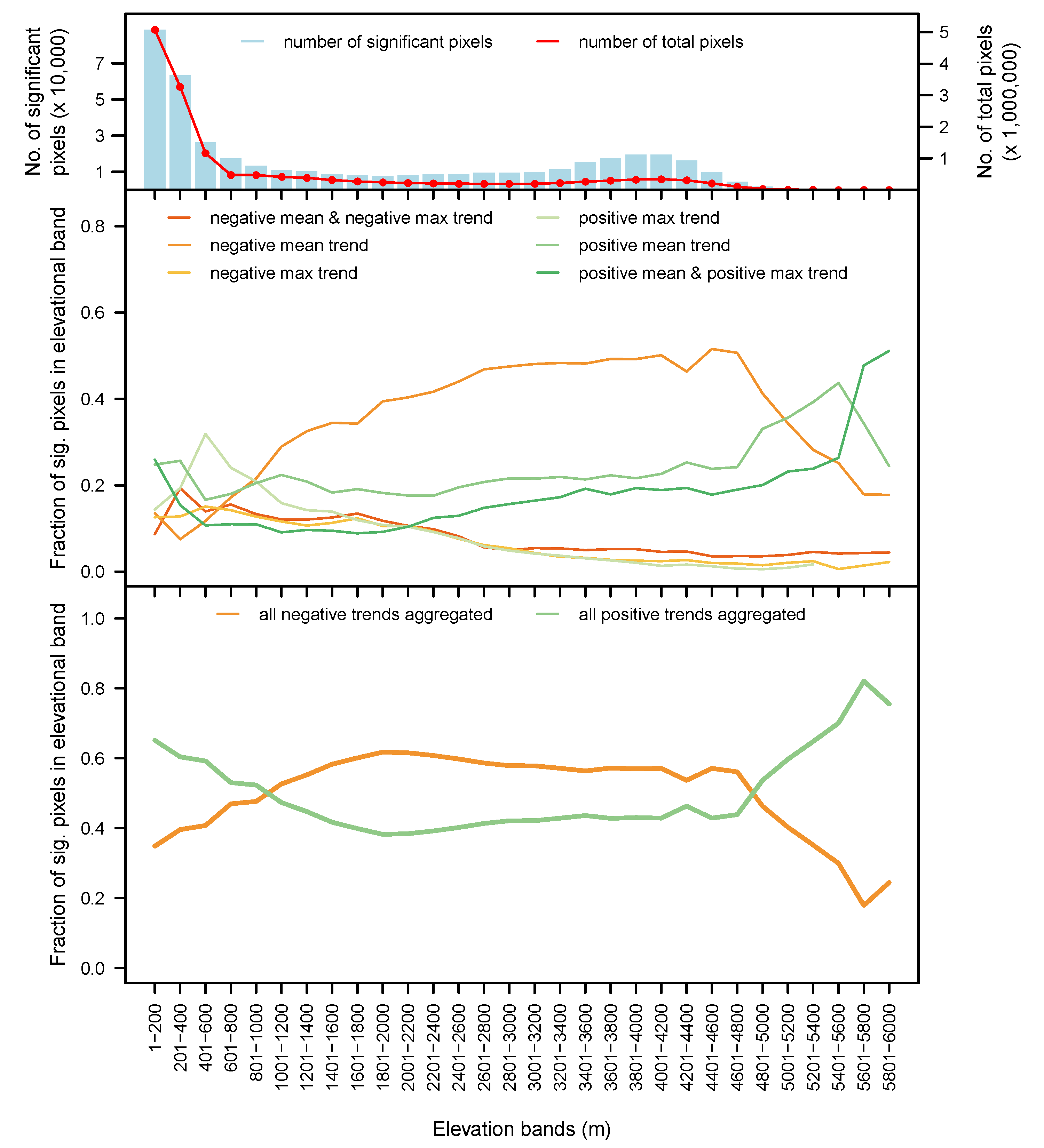
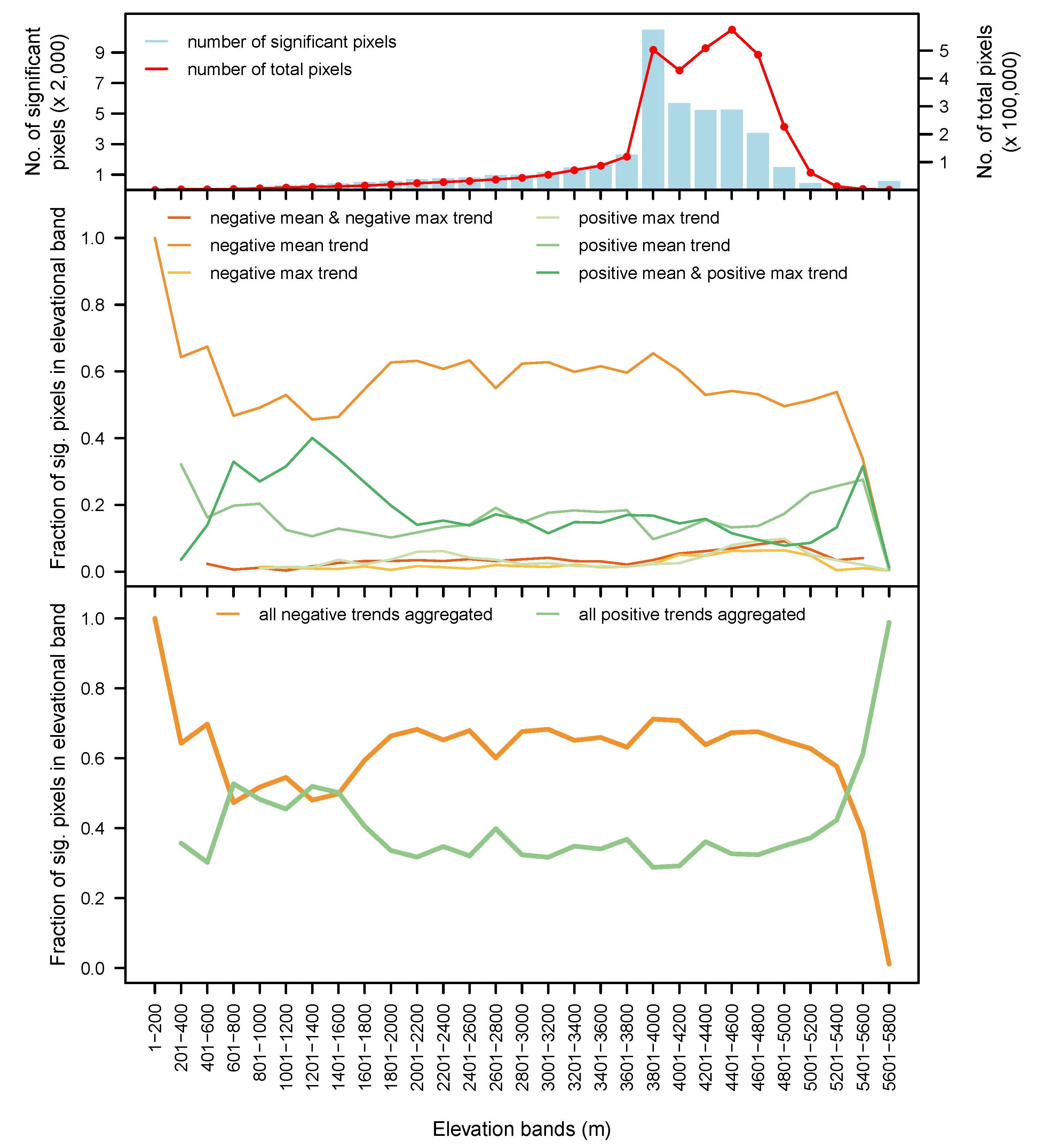
3.4. By Elevation
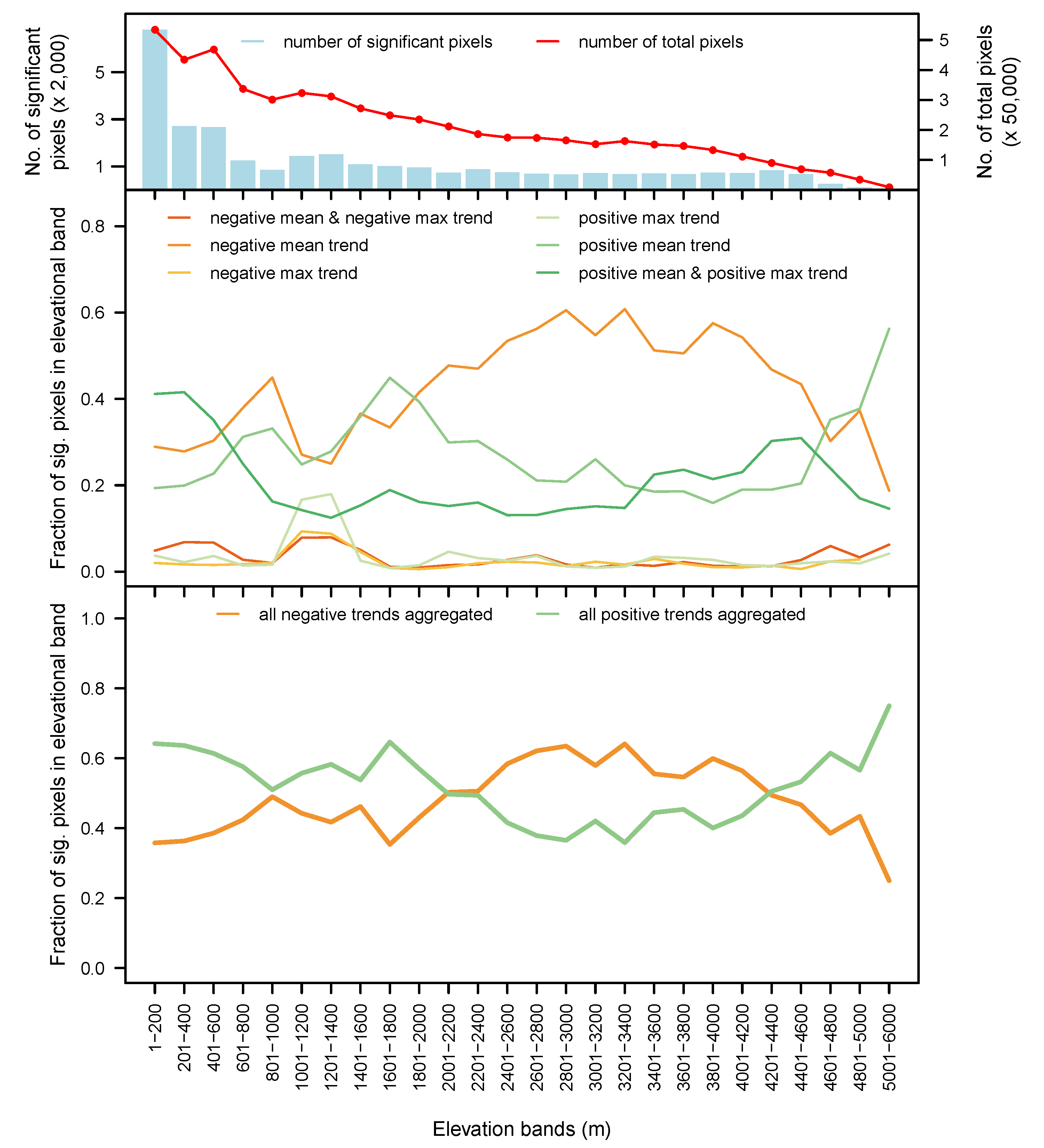
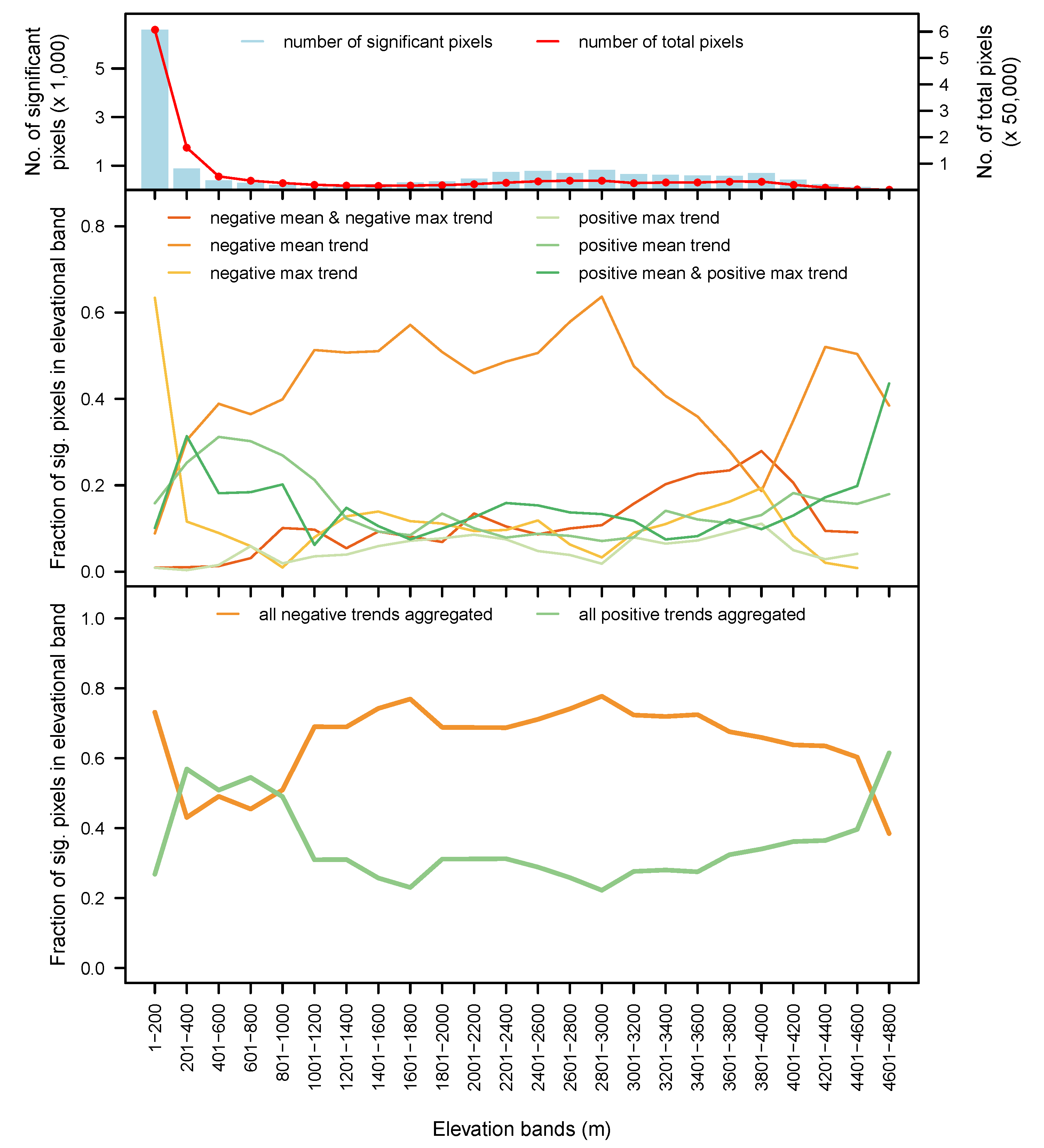
3.5. By Biome and Elevation
4. Discussion
4.1. Drivers of Greening and Browning Inside Protected Areas
4.2. Drivers of Greening and Browning by Biome and Elevation
4.3. Caveats and Additional Considerations
5. Conclusions
Author Contributions
Funding
Acknowledgments
Conflicts of Interest
References
- Von Humboldt, A. Views of the Cordilleras and Monuments of the Indigenous Peoples of the Americas; University of Chicago Press: Chicago, IL, USA, 2012. [Google Scholar]
- Von Humboldt, A. Political Essay on the Kingdom of New Spain; Volume 1, University of Chicago Press: Chicago, Il, USA, 2019. [Google Scholar]
- Von Humboldt, A. Political Essay on the Kingdom of New Spain; Volume 2, University of Chicago Press: Chicago, Il, USA, 2019. [Google Scholar]
- Von Humboldt, A.; Bonpland, A. Essay on the Geography of Plants; Jackson, S.T., Romanowski, S., Eds.; Reprint; University of Chicago Press: Chicago, IL, USA, 2009. [Google Scholar]
- Lack, H.W. Alexander von Humboldt: The Botanical Exploration of the Americas; Prestel: Munich, Germany, 2018. [Google Scholar]
- Zimmerer, K.S. Humboldt’s nodes and modes of interdisciplinary environmental science in the Andean world. Geogr. Rev. 2006, 96, 335–360. [Google Scholar] [CrossRef]
- Morueta-Holme, N.; Engemann, K.; Sandoval-Acuña, P.; Jonas, J.D.; Segnitz, R.M.; Svenning, J.-C. Strong upslope shifts in Chimborazo’s vegetation over two centuries since Humboldt. Proc. Natl. Acad. Sci. USA 2015, 112, 12741–12745. [Google Scholar] [CrossRef] [PubMed]
- Moret, P.; Muriel, P.; Jaramillo, R.; Dangles, O. Humboldt’s Tableau Physique revisited. Proc. Natl. Acad. Sci. USA 2019, 116, 12889–12894. [Google Scholar] [CrossRef] [PubMed]
- Schrodt, F.; Santos, M.J.; Bailey, J.J.; Field, R. Challenges and opportunities for biogeography—What can we still learn from von Humboldt? J. Biogeogr. 2019, 46, 1–12. [Google Scholar] [CrossRef]
- Millington, A.; Jepson, W. (Eds.) Land Change Science in the Tropics: Changing Agricultural Landscapes; Springer: New York, NY, USA, 2008. [Google Scholar]
- Boillat, S.; Scarpa, F.M.; Robson, J.P.; Gasparri, I.; Aide, T.M.; Aguiar, A.P.D.; Anderson, L.O.; Batistella, M.; Fonseca, M.G.; Futemma, C.; et al. Land system science in Latin America: Challenges and perspectives. Curr. Opin. Environ. Sustain. 2017, 26–27, 37–46. [Google Scholar] [CrossRef]
- Rodríguez, L.O.; Young, K.R. Biological diversity of Peru: Determining priority areas for conservation. AMBIO 2000, 29, 329–337. [Google Scholar] [CrossRef]
- Young, K.R.; Rodríguez, L.O. Development of Peru’s national protected area system: Historical continuity in conservation goals. In Globalization and New Geographies of Conservation; Zimmerer, K.S., Ed.; University of Chicago Press: Chicago, IL, USA, 2006; pp. 229–254. [Google Scholar]
- Aide, T.M.; Clark, M.L.; Grau, H.R.; López-Carr, D.; Levy, M.A.; Redo, D.; Bonilla-Moheno, M.; Riner, G.; Andrade-Núñez, M.J.; Muñiz, M. Deforestation and reforestation of Latin America and the Caribbean (2001–2010). Biotropica 2013, 45, 262–271. [Google Scholar] [CrossRef]
- Aide, T.M.; Grau, H.R.; Graesser, J.; Andrade-Nuñez, M.J.; Aráoz, E.; Barros, A.P.; Campos-Cerqueira, M.; Chacon-Moreno, E.; Cuesta, F.; Espinoza, R.; et al. Woody vegetation dynamics in the tropical and subtropical Andes from 2001 to 2014: Satellite image interpretation and expert validation. Glob. Change Biol. 2019, 25, 2112–2126. [Google Scholar] [CrossRef]
- Zhu, Z.; Piao, S.; Myneni, R.B.; Huang, M.; Zeng, Z.; Canadell, J.G.; Ciais, P.; Sitch, S.; Friedlingstein, P.; Arneth, A.; et al. Greening of the Earth and its drivers. Nat. Clim. Chang. 2016, 6, 791–795. [Google Scholar] [CrossRef]
- Chen, C.; Park, T.; Wang, X.; Piao, S.; Xu, B.; Chaturvedi, R.K.; Fuchs, R.; Brovkin, V.; Ciais, P.; Fensholt, R.; et al. China and India lead in greening of the world through land-use management. Nat. Sustain. 2019, 2, 122. [Google Scholar] [CrossRef]
- Parent, M.B.; Verbyla, D. The browning of Alaska’s boreal forest. Remote Sens. 2010, 2, 2729–2747. [Google Scholar] [CrossRef]
- De Jong, R.; Verbesselt, J.; Schaepman, M.E.; de Bruin, S. Trend changes in global greening and browning: Contribution of short-term trends to longer-term change. Glob. Chang. Biol. 2012, 18, 642–655. [Google Scholar] [CrossRef]
- Mishra, N.B.; Mainali, K.P. Greening and browning of the Himalaya: Spatial patterns and the role of climatic change and human drivers. Sci. Total Environ. 2017, 587, 326–339. [Google Scholar] [CrossRef] [PubMed]
- Houston, J.; Hartley, A.J. The central Andean west-slope rainshadow and its potential contribution to the origin of hyper-aridity in the Atacama Desert. Int. J. Climatol. 2003, 23, 1453–1464. [Google Scholar] [CrossRef]
- Garreaud, R.D. The Andes climate and weather. Adv. Geosci. 2009, 22, 3–11. [Google Scholar] [CrossRef]
- Young, K.R.; Leon, B.L.; Jorgensen, P.M.; Ulloa Ulloa, C. Tropical and subtropical landscapes of the Andes. In The Physical Geography of South America; Veblen, T.T., Young, K.R., Orme, A.R., Eds.; Oxford University Press: Oxford, UK, 2007; pp. 200–216. [Google Scholar]
- SERNANP Listado de Áreas Naturales Protegidas. Available online: http://www.sernanp.gob.pe/el-sinanpe (accessed on 16 July 2019).
- Kier, G.; Mutke, J.; Dinerstein, E.; Ricketts, T.H.; Küper, W.; Kreft, H.; Barthlott, W. Global patterns of plant diversity and floristic knowledge. J. Biogeogr. 2005, 32, 1107–1116. [Google Scholar] [CrossRef]
- Joppa, L.N.; Roberts, D.L.; Myers, N.; Pimm, S.L. Biodiversity hotspots house most undiscovered plant species. Proc. Natl. Acad. Sci. USA 2011, 108, 13171–13176. [Google Scholar] [CrossRef]
- Miraldo, A.; Li, S.; Borregaard, M.K.; Flórez-Rodríguez, A.; Gopalakrishnan, S.; Rizvanovic, M.; Wang, Z.; Rahbek, C.; Marske, K.A.; Nogués-Bravo, D. An Anthropocene map of genetic diversity. Science 2016, 353, 1532–1535. [Google Scholar] [CrossRef]
- Rau, P.; Bourrel, L.; Labat, D.; Melo, P.; Dewitte, B.; Frappart, F.; Lavado, W.; Felipe, O. Regionalization of rainfall over the Peruvian Pacific slope and coast. Int. J. Climatol. 2017, 37, 143–158. [Google Scholar] [CrossRef]
- Espinoza, J.C.; Chavez, S.; Ronchail, J.; Junquas, C.; Takahashi, K.; Lavado, W. Rainfall hotspots over the southern tropical Andes: Spatial distribution, rainfall intensity, and relations with large-scale atmospheric circulation. Water Resour. Res. 2015, 51, 3459–3475. [Google Scholar] [CrossRef]
- Didan, K.; Barreto Munoz, A.; Solano, R.; Huete, A. MODIS Vegetation Index User’s Guide; Version 3.00; Vegetation Index and Phenology Lab, The University of Arizona: Tucson, AR, USA, 2015. [Google Scholar]
- Savitzky, A.; Golay, M.J.E. Smoothing and differentiation of data by simplified least squares procedures. Anal. Chem. 1964, 36, 1627–1639. [Google Scholar] [CrossRef]
- Sen, P.K. Estimates of the regression coefficient based on Kendall’s tau. J. Am. Stat. Assoc. 1968, 63, 1379–1389. [Google Scholar] [CrossRef]
- Mann, H.B. Nonparametric tests against trend. Econom. J. Econom. Soc. 1945, 245–259. [Google Scholar] [CrossRef]
- Olson, D.M.; Dinerstein, E.; Wikramanayake, E.D.; Burgess, N.D.; Powell, G.V.; Underwood, E.C.; D’Amico, J.A.; Itoua, I.; Strand, H.E.; Morrison, J.C. Terrestrial ecoregions of the world: A new map of life on Earth. BioScience 2001, 51, 933–938. [Google Scholar] [CrossRef]
- Antonelli, A.; Zizka, A.; Carvalho, F.A.; Scharn, R.; Bacon, C.D.; Silvestro, D.; Condamine, F.L. Amazonia is the primary source of Neotropical biodiversity. Proc. Natl. Acad. Sci. USA 2018, 115, 6034–6039. [Google Scholar] [CrossRef] [PubMed]
- Lü, Y.; Zhang, L.; Feng, X.; Zeng, Y.; Fu, B.; Yao, X.; Li, J.; Wu, B. Recent ecological transitions in China: Greening, browning, and influential factors. Sci. Rep. 2015, 5, 8732. [Google Scholar] [CrossRef]
- Murillo-Sandoval, P.J.; Van Den Hoek, J.; Hilker, T. Leveraging multi-sensor time series datasets to map short- and long-term tropical forest disturbances in the Colombian Andes. Remote Sens. 2017, 9, 179. [Google Scholar] [CrossRef]
- Buitenwerf, R.; Sandel, B.; Normand, S.; Mimet, A.; Svenning, J.-C. Land surface greening suggests vigorous woody regrowth throughout European semi-natural vegetation. Glob. Chang. Biol. 2018, 24, 5789–5801. [Google Scholar] [CrossRef]
- Chazdon, R.L. Second Growth: The Promise of Tropical Forest Regeneration in an Age of Deforestation; University of Chicago Press: Chicago, IL, USA, 2014. [Google Scholar]
- Young, K.R. Ecology of land cover change in glaciated tropical mountains. Rev. Peru. Biol. 2014, 21, 259–270. [Google Scholar]
- Young, K.R.; Ponette-González, A.G.; Polk, M.H.; Lipton, J.K. Snowlines and treelines in the tropical Andes. Ann. Am. Assoc. Geogr. 2017, 107, 429–440. [Google Scholar] [CrossRef]
- Kintz, D.B.; Young, K.R.; Crews-Meyer, K.A. Implications of land use/land cover change in the buffer zone of a national park in the tropical Andes. Environ. Manag. 2006, 38, 238–252. [Google Scholar] [CrossRef] [PubMed]
- Lipton, J.K. Human Dimensions of Conservation, Land Use, and Climate Change in Huascaran National Park, Peru. Ph.D. Thesis, University of Texas at Austin, Austin, TX, USA, 2008. [Google Scholar]
- Rehm, E.M.; Feeley, K.J. Forest patches and the upward migration of timberline in the southern Peruvian Andes. For. Ecol. Manag. 2013, 305, 204–211. [Google Scholar] [CrossRef]
- Mazzarino, M.; Finn, J.T. An NDVI analysis of vegetation trends in an Andean watershed. Wetlands Ecol. Manag. 2016, 24, 623–640. [Google Scholar] [CrossRef]
- Radel, C.; Jokisch, B.D.; Schmook, B.; Carte, L.; Aguilar-Støen, M.; Hermans, K.; Zimmerer, K.; Aldrich, S. Migration as a feature of land system transitions. Curr. Opin. Environ. Sustain. 2019, 38, 103–110. [Google Scholar] [CrossRef]
- Bury, J.; Mark, B.G.; Carey, M.; Young, K.R.; McKenzie, J.; Baraer, M.; French, A.; Polk, M.H. New geographies of water and climate change in Peru: Coupled natural and social transformations in the Santa River watershed. Ann. Assoc. Am. Geogr. 2013, 103, 363–374. [Google Scholar] [CrossRef]
- Carey, M.; Baraer, M.; Mark, B.G.; French, A.; Bury, J.; Young, K.R.; McKenzie, J.M. Toward hydro-social modeling: Merging human variables and the social sciences with climate-glacier runoff models (Santa River, Peru). J. Hydrol. 2014, 518, 60–70. [Google Scholar] [CrossRef]
- Van Leeuwen, W.J.D.; Hartfield, K.; Miranda, M.; Meza, F.J. Trends and ENSO/AAO driven variability in NDVI derived productivity and phenology alongside the Andes Mountains. Remote Sens. 2013, 5, 1177–1203. [Google Scholar] [CrossRef]
- Panigada, C.; Tagliabue, G.; Zaady, E.; Rozenstein, O.; Garzonio, R.; Di Mauro, B.; De Amicis, M.; Colombo, R.; Cogliati, S.; Miglietta, F.; et al. A new approach for biocrust and vegetation monitoring in drylands using multi-temporal Sentinel-2 images. Prog. Phys. Geogr.: Earth Environ. 2019, 43, 496–520. [Google Scholar] [CrossRef]
- Fensholt, R.; Horion, S.; Tagesson, T.; Ehammer, A.; Ivits, E.; Rasmussen, K. Global-scale mapping of changes in ecosystem functioning from earth observation-based trends in total and recurrent vegetation. Glob. Ecol. Biogeogr. 2015, 24, 1003–1017. [Google Scholar] [CrossRef]
- Eastman, J.R.; Sangermano, F.; Ghimire, B.; Zhu, H.; Chen, H.; Neeti, N.; Cai, Y.; Machado, E.A.; Crema, S.C. Seasonal trend analysis of image time series. Int. J. Remote Sens. 2009, 30, 2721–2726. [Google Scholar] [CrossRef]
- Verbesselt, J.; Hyndman, R.; Newnham, G.; Culvenor, D. Detecting trend and seasonal changes in satellite image time series. Remote Sens. Environ. 2010, 114, 106–115. [Google Scholar] [CrossRef]
- Tote, C.; Beringhs, K.; Swinnen, E.; Govers, G. Monitoring environmental change in the Andes based on SPOT-VGT and NOAA-AVHRR time series analysis. In Proceedings of the 6th International Workshop on the Analysis of Multi-temporal Remote Sensing Images (IEEE 2011), Trento, Italy, 12–14 July 2011; pp. 268–272. [Google Scholar]
- Zimmer, A.; Meneses, R.I.; Rabatel, A.; Soruco, A.; Dangles, O.; Anthelme, F. Time lag between glacial retreat and upward migration alters tropical alpine communities. Perspect. Plant Ecol. Evolut. Syst. 2018, 30, 89–102. [Google Scholar] [CrossRef]
- Sugihara, G.; May, R.; Ye, H.; Hsieh, C.; Deyle, E.; Fogarty, M.; Munch, S. Detecting causality in complex ecosystems. Science 2012, 338, 496–500. [Google Scholar] [CrossRef] [PubMed]
- Mainali, K.; Bewick, S.; Vecchio-Pagan, B.; Karig, D.; Fagan, W.F. Detecting interaction networks in the human microbiome with conditional Granger causality. PLoS Comput. Biol. 2019, 15, e1007037. [Google Scholar] [CrossRef]


| Trend Type |  | Confidence Level |
| Both Positive | Highest Greening | |
| Positive Mean NDVI | Robust Greening | |
| Positive Max NDVI | Strong Greening | |
| Negative Max NDVI | Strong Browning | |
| Negative Mean NDVI | Robust Browning | |
| Both Negative | Highest Browning |
| Trend Type | Area (km2) | % of Pixels with Significant Trend |
|---|---|---|
| Both Positive | 6448.3 | 18.7 |
| Positive Mean NDVI | 7257.1 | 21.1 |
| Positive Max NDVI | 11,539.1 | 33.5 |
| Negative Max NDVI | 3005.9 | 8.7 |
| Negative Mean NDVI | 2766.0 | 8.0 |
| Both Negative | 3380.7 | 9.8 |
| Total | 34,398 | 100 |
© 2020 by the authors. Licensee MDPI, Basel, Switzerland. This article is an open access article distributed under the terms and conditions of the Creative Commons Attribution (CC BY) license (http://creativecommons.org/licenses/by/4.0/).
Share and Cite
Polk, M.H.; Mishra, N.B.; Young, K.R.; Mainali, K. Greening and Browning Trends across Peru’s Diverse Environments. Remote Sens. 2020, 12, 2418. https://doi.org/10.3390/rs12152418
Polk MH, Mishra NB, Young KR, Mainali K. Greening and Browning Trends across Peru’s Diverse Environments. Remote Sensing. 2020; 12(15):2418. https://doi.org/10.3390/rs12152418
Chicago/Turabian StylePolk, Molly H., Niti B. Mishra, Kenneth R. Young, and Kumar Mainali. 2020. "Greening and Browning Trends across Peru’s Diverse Environments" Remote Sensing 12, no. 15: 2418. https://doi.org/10.3390/rs12152418
APA StylePolk, M. H., Mishra, N. B., Young, K. R., & Mainali, K. (2020). Greening and Browning Trends across Peru’s Diverse Environments. Remote Sensing, 12(15), 2418. https://doi.org/10.3390/rs12152418