Article

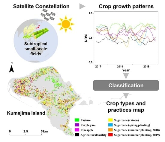
Satellite Constellation Reveals Crop Growth Patterns and Improves Mapping Accuracy of Cropping Practices for Subtropical Small-Scale Fields in Japan

1
Graduate School of Systems and Information Engineering, University of Tsukuba, 1-1-1 Tennodai, Tsukuba, Ibaraki 305-8577, Japan
2
Center for Environmental Biology and Ecosystem Studies, National Institute for Environmental Studies, 16-2 Onogawa, Tsukuba, Ibaraki 305-8506, Japan
*
Author to whom correspondence should be addressed.
Remote Sens. 2020, 12(15), 2419; https://doi.org/10.3390/rs12152419
Submission received: 9 June 2020 / Revised: 16 July 2020 / Accepted: 26 July 2020 / Published: 28 July 2020

Abstract

:
Mapping of agricultural crop types and practices is important for setting up agricultural production plans and environmental conservation measures. Sugarcane is a major tropical and subtropical crop; in general, it is grown in small fields with large spatio-temporal variations due to various crop management practices, and satellite observations of sugarcane cultivation areas are often obscured by clouds. Surface information with high spatio-temporal resolution obtained through the use of emerging satellite constellation technology can be used to track crop growth patterns with high resolution. In this study, we used Planet Dove imagery to reveal crop growth patterns and to map crop types and practices on subtropical Kumejima Island, Japan (lat. 26°21′01.1″ N, long. 126°46′16.0″ E). We eliminated misregistration between the red-green-blue (RGB) and near-infrared band imagery, and generated a time series of seven vegetation indices to track crop growth patterns. Using the Random Forest algorithm, we classified eight crop types and practices in the sugarcane. All the vegetation indices tested showed high classification accuracy, and the normalized difference vegetation index (NDVI) had an overall accuracy of 0.93 and Kappa of 0.92 range of accuracy for different crop types and practices in the study area. The results for the user’s and producer’s accuracy of each class were good. Analysis of the importance of variables indicated that five image sets are most important for achieving high classification accuracy: Two image sets of the spring and summer sugarcane plantings in each year of a two-year observation period, and one just before harvesting in the second year. We conclude that high-temporal-resolution time series images obtained by a satellite constellation are very effective in small-scale agricultural mapping with large spatio-temporal variations.

Graphical Abstract

1. Introduction

Agricultural land is a key component of land use and land cover. Nearly 40% of the Earth’s land surface is now being used for agriculture [1]. The expansion of agricultural land to increase food production and intensification of its use [2] has altered the structure and function of ecosystems and in some cases has diminished their ability to continue providing valuable resources [1,3,4]. Many land management applications require reliable and timely land cover mapping over large heterogeneous landscapes [5]. Therefore, mapping and monitoring of agricultural land use is an important topic of high public interest.
The use of satellite remote sensing to monitor the use and management of agricultural land over a large area is an efficient approach (e.g., [6,7,8,9,10,11,12,13,14,15,16,17]). In agricultural mapping, vegetation indices are used to capture the unique growth pattern of each crop, and high classification accuracy has been achieved by using multi-temporal imagery [10]. Multi-temporal Landsat data (spatial resolution = 30 m) has been used in phenological analyses of various regions with varied land cover (e.g., [16,18,19,20,21]). However, Landsat satellites (ex. TM, ETM+) collect data every 16 days, which makes it difficult to capture agricultural events in some regions [22], because clouds often hamper image acquisition. According to Whitcraft et al. (2015) [23], the potential for cloud cover is particularly high and agricultural events are hard to capture using existing optical satellite observation networks in Southeast Asia, Southwest Africa, and Central America, where agriculture relies on rainfall. Consequently, attention has been paid to high-frequency observation satellites (e.g., MODerate resolution Imaging Spectroradiometer (MODIS); spatial resolution = 250 m), and an agricultural monitoring method that uses high-temporal-resolution data has been developed [7,14,24,25,26,27]. However, there is a fundamental limit to the spatial scale of the agricultural field that can be monitored due to the effects of mixed pixels resulting from the lower spatial resolution that is a trade-off with higher temporal resolution. In particular, many regions with frequent cloud cover have small agricultural areas (<2 ha) [28,29], which cannot be reliably visualized using these data.
Sugarcane is grown mainly in large-scale production areas such as Brazil, but its cultivation is also possible in small areas on tropical and subtropical islands, where it is a major crop [30,31]. These areas have high cloud cover potential which makes surface information imaging problematic [28,29]. In such areas, sugarcane production planning is the main concern from the point of view of employment [32]. In Okinawa, Japan, sugarcane is the main crop, and production planning is a primary concern [33]. Soil runoff from sugarcane fields has a great impact on rivers and coastal ecosystems [34], and cropping practices greatly affect its spatio-temporal fluctuations [35]. Therefore, it is important to understand the spatial distribution of crop types in fields, as well as sugarcane cropping practices, for both agricultural production planning and environmental conservation measures [36]. To achieve this understanding, tracking crop growth patterns and mapping crop types and practices by remote sensing is required. However, the crop types classification of sugarcane area in Japan does not provide satisfactory accuracy in previous study [37]. In addition, sugarcane cropping practices has not been classified.
Sugarcane has a relatively long harvest period (approximately 3 months) and multiple management practices, and the spatio-temporal variations are large [38,39]. Therefore, monitoring sugarcane by using satellite remotely sensed data is limited by spatio-temporal resolution [38]. Heterogeneous agricultural landscapes are characterized by land cover categories that can be difficult to separate spectrally due to low inter-class separability and high intra-class variability in a single image [5]. At the same time, observation with high spatial resolution is required [40], because many sugarcane fields are small (<2 ha). Therefore, both high-frequency and high-spatial-resolution data are required for classifying crop types and practices in agricultural land that includes sugarcane fields [39].
Recently, satellite constellations constructed by launching a large number of identical small satellites have attracted attention as systems that achieve both high temporal (every day) and high spatial resolution (3 m). Planet Labs, Inc. operates the largest satellite constellation, with Dove nano-satellites collecting multi-band (blue, green, red, and near-infrared) images of the entire land surface of the Earth every day; collection capacity is 200 million km2/day, based on a full constellation of approximately 130 satellites [41]. Owing to the huge number of images obtained, the opportunities for change detection and surface characterization are enormous, which encourages application of this approach to agricultural monitoring [42,43,44,45,46]. Understanding the crop growth pattern revealed by high-frequency and high-resolution observations may reveal the optimal observation dates for crop types and practices classification.
The purpose of this study was to classify crop types and practices (i.e., sugarcane (ratoon), sugarcane (spring planting), sugarcane (summer planting in 2018), sugarcane (summer planting in 2019), pasture, purple yam, pineapple and agricultural facility) on a subtropical island by using crop growth patterns estimated from satellite constellation data of high temporal and spatial resolution and to identify the most effective dates for undertaking the classification.

2. Materials and Methods
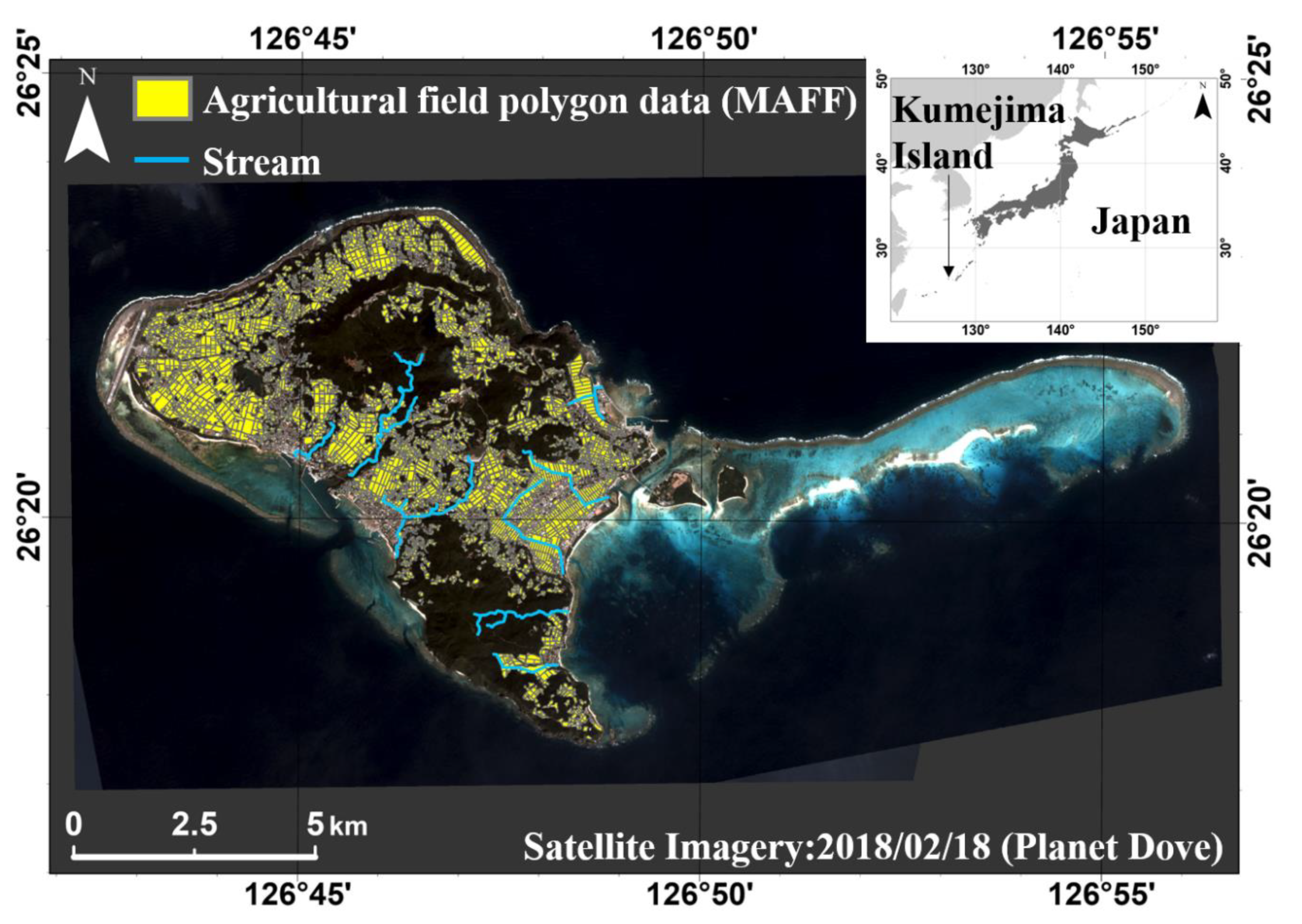
2.1. Study Area

Kumejima Island (59 km2) is about 100 km west of the main Okinawa Island (Figure 1) and is located in a subtropical climate [36]. The mean annual air temperature is 23.0 °C, annual rainfall is 2111.8 mm, 44% of which falls in the rainy season from May to June or is associated with typhoons in August and September (Japan Meteorological Agency, http://www.data.jma.go.jp/obd/stats/etrn/). The central part of the island is composed of volcanic rock and reaches a maximum altitude of 310 m above sea level [36,47].
The study area was an agricultural area of 17.1 km2 (Ministry of Agriculture, Forestry and Fisheries, Japan, MAFF; https://www.maff.go.jp/j/tokei/kouhyou/sakumotu/menseki/#c), which is covered by sugarcane, pasture, purple yam, pineapple, agricultural facilities such as greenhouses, and other crops such as squash, okra, and rice. Sugarcane is the predominant crop [36]. On Kumejima Island, there are three key sugarcane management practices (Table 1): (1) Ratooning, in which sugarcane grows from sprouts of underground stubble left in the field after harvest of the main crop (i.e., ratoon), and is harvested about every 12 months, usually for at least 4 years, and then the crop is renewed due to decreasing yield; (2) spring planting of seedlings (between February and May, just after harvesting); and (3) summer planting of seedlings (between July and October). The sugar industry equipment usually operates from January to March. In ratooning, sugarcane is harvested 12 months after harvesting in previous year, in spring planting it is harvested 12 months after planting, and in summer planting it is harvested in the sugar-production period 18 months after planting. About 63% of farmers manage a sugarcane area of less than 1 ha [48].
Cultivation of purple yam for confectionery products and as feed for meat calf husbandry is also active, and new pastures are being developed in some parts of the island. Pineapples were cultivated extensively on the island in the 1960s and 1970s, but are now grown only by some farmers and in private gardens. Flowers, bitter gourd, mango, and banana are cultivated in agricultural facilities such as greenhouses. Precise classification is required for various crop type fields on the island; this need also provides us an opportunity to evaluate the performance of classification of crop types and practices using high-frequency and high-spatial imagery from a satellite constellation.

2.2. Dove Satellite Image Pre-Processing

Planet Dove imagery was obtained from Planet Explorer (https://www.planet.com/explorer/) and processed as shown in Figure 2. The image product is delivered as a continuous, split-frame strip, with half-frames containing red-green-blue (RGB) and near-infrared (NIR) imagery, with an observation interval of approximately 0.5 s [49].
We used Dove ortho scenes (Planet Labs image product Level 3B: 4-Band PlanetScope Scene; spatial resolution = 3 m) from 1 July 2017 to 31 December 2019, which are orthorectified and radiometrically and sensor corrected. The geometric correction was based on digital elevation models with post-spacing between 30 and 90 m, with a root mean square error specification of <10 m [41]. We removed bad pixels using the unusable data mask provided with the products. We converted radiance to top-of-atmospheric reflectance using the scaling factor provided with the products. Dove satellites have been observed by two sensor types: Conventional type (PS2) and next-generation type (PS2.SD). Since these sensors have different relative spectral response curves, we transformed the next-generation-type values to match those of the conventional type using the coefficient described in the metadata.
Mismatches in the band-to-band registration were confirmed by visual inspection, and all images were re-registered by the zero-mean normalized cross-correlation method [50] with edge enhancing by a Laplacian filter; images with a shift of more than 10 pixels were excluded from the analysis. To maintain the continuity of pixel-based time series change, the registration between images was processed by the same method as the band-to-band re-registration, and was based on the reference image with an accurate position; images with a shift of more than 10 m were excluded from the analysis.
We performed simple dark pixel subtraction to obtain surface reflectance [51]. Assuming the presence of a pixel with zero reflectance (i.e., the radiance recorded by the sensor is solely from atmospheric scattering), the minimum pixel value was subtracted from those of all other pixels to remove the radiance derived from atmospheric scattering. Pixels from deep ocean areas were used for this correction. In addition, we normalized the value of each band according to Ono et al. (2002) [52] by dividing it by the summed value of all bands. Even on the same ground surface, the spectra observed by the satellite vary considerably because of the influence of the surface slope and atmospheric effects, but the shape of the spectra can be regarded as similar [52]. This characteristic allows suppression of the topographic and atmospheric effects by normalizing with the total sum of reflectance [53].
These pre-processed Planet Dove images were also used to evaluate the temporal variation of the pixels available for analysis. Specifically, the acquisition rates of analyzable pixels (i.e., not cloud pollution pixels) in the five days composite image were calculated.

2.3. Time Series of Vegetation Indices

The vegetation indices are highly correlated with the biomass of vegetation, and their temporal changes represent the growth pattern of crops [54]. NIR is the spectral region most responsive to changes in vegetation density [42]. Rouse et al. (1974) [55] and Tucker (1979) [56] developed the normalized difference vegetation index (NDVI), which is based on NIR and red bands and is widely used. The soil-adjusted vegetation index (SAVI) [57], modified soil-adjusted vegetation index (MSAVI) [58], and enhanced vegetation index (EVI) [59] were all developed on the basis of NDVI. However, the usefulness of evaluating the vegetation temporal change pattern by using indices based on the visible bands has also been demonstrated [60]. In Planet Dove satellite images with a split-frame strip, observation times differ between RGB and NIR bands, which may result in misregistration (see above). Thus, it is also necessary to consider vegetation indices that use visible wavelengths only. These include the visible atmospherically resistant index (VARI) [17], green–red ratio vegetation index (GRVI) [61,62], and normalized green ratio (GR) [60]. We calculated the following seven vegetation indices from pre-processed Dove satellite images to create a vegetation index time series:
N D V I = ( ρ N I R ρ R e d ) / ( ρ N I R + ρ R e d )
S A V I = { ( 1 0.5 ) × ( ρ N I R ρ R e d ) } / ( ρ N I R + ρ R e d + 0.5 )
M S A V I = { 2 × ρ N I R + 1 ( 2 × ρ N I R + 1 ) 2 8 × ( ρ N I R ρ R e d ) } / 2
E V I = 2.5 × ( ρ N I R ρ R e d ) / ( ρ N I R + 6 × ρ R e d 7.5 × ρ B l u e + 1 )
V A R I = ( ρ G r e e n ρ R e d ) / ( ρ G r e e n + ρ R e d ρ B l u e )
G R V I = ( ρ G r e e n ρ R e d ) / ( ρ G r e e n + ρ R e d )
G R = ρ G r e e n / ( ρ R e d + ρ G r e e n + ρ B l u e )
where ρ B l u e , ρ G r e e n , ρ R e d and ρ N I R are Planet Dove blue, green, red, and near-infrared band reflectance, respectively.
To suppress atmospheric noise, we applied the best index slope extraction (BISE) algorithm [63] and refined the time series data of the vegetation indices. The search range was set to 40 days for 10-day composite data (the missing periods were linearly interpolated), considering the observation frequency and agricultural calendar in the target area. To deal with unequal observation intervals in the 10-day composite data, we used an integrated algorithm based on BISE and the maximum value interpolated (MVI) algorithm [64] to refine the vegetation index time series data on a daily basis.

2.4. Ground Truthing

Agricultural field polygon data were obtained from the Ministry of Agriculture, Forestry and Fisheries, Japan (available at: https://www.maff.go.jp/j/tokei/porigon/) and used to draw the shape of each parcel of agricultural land on satellite images (Figure 1). To gather reference data (i.e., training and validation data) for image classification, we conducted field surveys in the study area. Crop types and land cover conditions were recorded in each field and period (November 2018 and February, May, July, and October 2019). Main crop types and practices were recorded to the agricultural field polygon data. The following classes were used: (1) Sugarcane (ratoon), (2) sugarcane (spring planting), (3) sugarcane (summer planting in 2018), (4) sugarcane (summer planting in 2019), (5) pasture, (6) purple yam, (7) pineapple, (8) agricultural facility (e.g., vinyl greenhouse).
The use of available agricultural field boundary data improved the accuracy of classification because it allowed us to eliminate the effect of spectral variability within the agricultural field and the mixed-pixel effect [65]. Therefore, we used the agricultural field polygon data and extracted pure pixels corresponding only to the agricultural land. Sample sizes of reference data sets for each class were: (1) 36,902, (2) 12,671, (3) 17,743, (4) 2897, (5) 55,335, (6) 6628, (7) 874, and (8) 4281 pixels.

2.5. Classification and Accuracy Assessment

Considering the growing periods of pineapple and summer planting of sugarcane, the time series should span multiple years [37]. We used the time series data between 1 August 2017 and 30 November 2019 to generate a dataset for classification and validation. In the analysis of high-dimensional datasets, machine learning classification yields better results than the parametric classification algorithms do [66]. In particular, Random Forest (RF) [67] classification performs well without the need for complicated initial parameters, and is frequently used in land cover classification based on remote sensing data [68,69,70,71]. In general, machine learning algorithms, including RF, can be considered as black-box-type classifiers: The split rules for classification by RF are unknown [5], but RF can indicate the degrees of importance of variables for the general classification by the mean decrease in the Gini index [5]. The greater this decrease, the more important the variable is in the performance of the classification model. The relative importance of each variable was evaluated by normalizing to the sum of the mean decreases in the Gini index of all variables obtained during the classification model construction based on RF; this sum was considered to be 1. Such estimation is important for choosing appropriate dates for images that should be used to classify fields with high spatio-temporal variability. Therefore, we adopted RF to classify crop types and practices. For model development, tuning, and accuracy assessment, we used the add-on packages within version 3.6.1 of the 64-bit version of R [72]. The randomForest package [73] was used to build classifications with RF.
The classification parameters were set as follows. (1) The size of the training data was set to 500; this choice was based on our preliminary test with different sizes of the training data (n = 100, 200, 300, 400, 500). (2) The number of trees (ntree) was set to 500 after preliminary verification, in line with common practice [74]. (3) The other adjustable RF tuning parameter, mtry, controls the number of variables randomly considered at each split during tree building, and performance of RF is believed to be “somewhat sensitive” to this parameter [75]. The default value of mtry is the square root of p, where p equals the number of predictor variables within a dataset [73]. Generally, the default value is used [74], but in this study, mtry was tuned by the tuneRF function.
Classifications and validations of each vegetation index time series were conducted 10 times, each creating a confusion matrix. Training data were randomly sampled from the dataset (500 pixels in each class). Validation data were randomly sampled from a dataset that was not used as training data according to the area ratio of the class in the classification map (class of minimum area ratio was 30). Then the confusion matrix was used to calculate the evaluation indices: Overall accuracy (OA), producer’s accuracy of each class, user’s accuracy of each class, and Κappa [76]. Kappa is defined as:
K a p p a = ( P o P e ) / ( 1 P e )
where P o is the proportion of cases correctly classified (i.e., overall accuracy) and P e is the expected proportion of cases correctly classified by chance [77]. The Kappa ranges from −1 to +1, where +1 indicates perfect agreement, and values of zero or less indicate a performance no better than random [78]. The Kappa has been traditionally used in accuracy assessment for classification map based on remote sensing. One such interpretation scale that has been widely used in remote sensing applications is that proposed by Landis and Koch (1977) [79] criteria [77]: Poor for negative Kappa values, slight for 0.00 < Kappa 0.20, fair for 0.20 < Kappa 0.40, moderate for 0.40 < Kappa 0.60, substantial for 0.60 <  Kappa  0.80, and almost perfect for >0.80.

3. Results

3.1. Band-To-Band Re-Registration of Planet Dove Satellite Images

Figure 3 shows the results of validation of the original band-to-band registration. Misregistration between RGB bands was observed in images with heavy cloud cover, images of the sea, and images taken by the next-generation sensor types (PS2.SD); this sensor took about 1% of all images analyzed. Misregistration was not observed in clear land images taken by the conventional sensor types (PS2). Therefore, no re-registration between RGB bands was performed for images taken with the PS2 sensors, and images taken by PS2.SD sensors were removed from the analysis. In many images, misregistration was seen between the RGB and NIR bands; these images were re-registered by matching the NIR band image to the RGB band image.

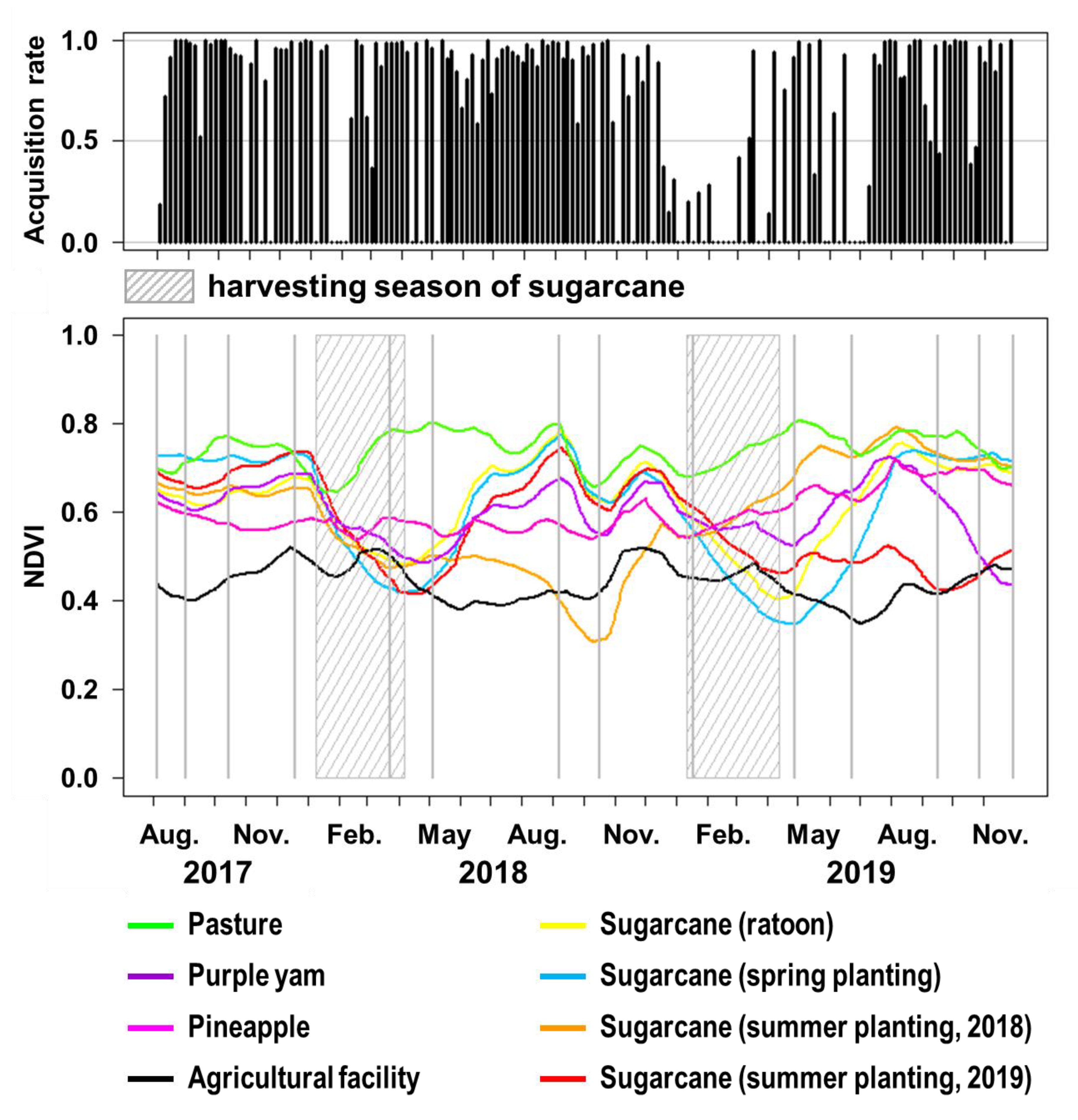
3.2. Crop Growth Patterns Estimated by Planet Dove Imagery

Figure 4 shows the average NDVI time series of each crop type and practice in the field survey area created from the Planet Dove images. These series represent the crop growth patterns of each crop type and practice. Ratooning and spring planting of sugarcane had a similar crop growth pattern. In the summer planting of sugarcane, changes in the percentage of vegetation cover with time differed greatly from those in ratooning and spring planting. Pastures had high NDVI values throughout the year. Pineapple had a lower NDVI value throughout the year than did pastures. Agricultural facilities had lower NDVI values than any crop types and practices. The NDVI value of purple yam peaked in July, then decreased gradually, and was lowest in November. While the acquisition rates of the original NDVI values based on Planet Dove imagery were low from January to February and in June, spectra related to land cover information were usually obtained within 5 to 10 days for the rest of the periods.

3.3. Mapping and Classification Accuracy of Crop Types and Practices Using NDVI Time Series

Figure 5 shows the classification accuracy of each vegetation index time series evaluated from 10 random samplings of training data. High classification accuracy was obtained with all vegetation indices (Figure 5). All vegetation indices have an average OA exceeding 0.91, and the average Kappa exceeding 0.89. Vegetation indices based on both visible and NIR bands (NDVI, SAVI, MSAVI, and EVI) provided slightly better classification accuracy than those based on visible bands only (VARI, GRVI, and GR). This can be confirmed by the threshold based on the average value of classification by all vegetation indices (red line in Figure 5). No significant difference was found between NDVI and other vegetation indices based on visible and NIR bands. This suggested that the NIR band, which reflects vegetation better than visible wavelengths [80], could be effectively used after band-to-band re-registering. Because NDVI did not differ from other NIR-based vegetation indices, we recommend the traditional and versatile NDVI classification.
We created a crop type and practice map using the NDVI time series (Figure 6). In this map, the class with the maximum average value of the class probabilities when the classification was conducted 10 times by RF. Class probability indicates the probability that a pixel belongs to each class when classified by RF. Even though classification in this map was on a pixel basis, the segments of crop types and practices were adequately represented in most of the agricultural parcels.
We compared the percentage of pure pixels that can be classified with the Planet Dove imagery with other representative medium-resolution satellite images. The ratio of pure pixel area to agricultural land area (agricultural field polygon data) was 85.2% in Planet Dove imagery (spatial resolution, 3 m), 55.5% in Sentinel-2 (10 m), and 11.3% in Landsat images (30 m). The presence or absence of target pixels in the polygon data was 99.8% in Planet Dove imagery, 90.3% in Sentinel-2 imagery, and 16.4% in Landsat imagery.
Table 2 shows a confusion matrix that combines the results of 10 trials of classification using the NDVI time series. The classification accuracy of crop type and practice using NDVI time series was 0.93 for OA and 0.92 for Kappa (Table 2). The accuracy of classification into sugarcane vs. others was 0.98 for OA and 0.97 for Kappa. The producer’s accuracy and user’s accuracy of sugarcane were 0.98 and 0.99 respectively, and the other’s were 0.99 and 0.98 respectively. This result is superior to the published values of OA (0.84–0.96) and Kappa (0.59–0.87) obtained using remotely sensed satellite imagery (combination of Formosat/MS, ALOS/AVNIR2, SPOT/HRV and HRG [37], combination of Landsat sensors [81,82], MODIS [83]). However, it should be noted that the previous studies were not necessarily limited to crop type classification as in this study (for example, forests were included in other class [37]).

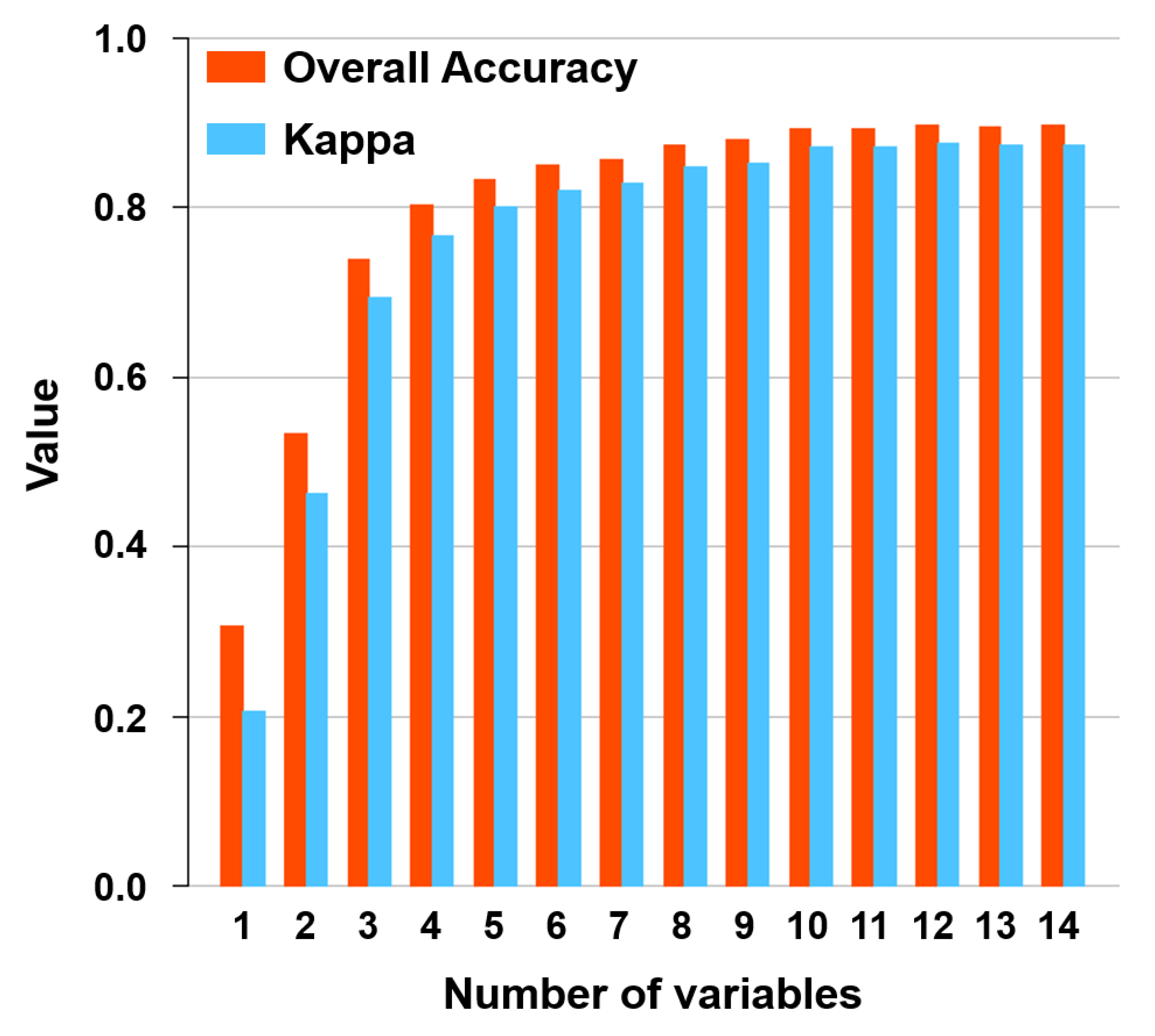
3.4. Assessment of the Optimal Dates and Required Observation Periods for Classification

Figure 7 shows the time series changes in the importance of variables based on normalized reduction of Gini; the importance seemed to have a seasonal variation. The peak days of time series with 10-day intervals coincided with the timing of crop planting and harvesting (Figure 4). Figure 8 shows the normalized mean decrease of Gini reassessed by classification using only NDVI images of 14 peak days. We found that classification accuracy varied with the number of images used for crop type and practice classification (Figure 9), where the variables used were added from the date with the most variable importance (i.e., normalized mean decrease Gini) shown in Figure 8.

4. Discussion

4.1. Band-To-Band Registration of Planet Dove Satellite Images

The deliberately inexpensive sensor designs and commercial off-the-shelf components of small satellites worsen the consistency of acquired data quality in comparison with that of traditional large satellites [42]. Measurements over slightly mismatched areas from different spectral bands lead to much less accurate science data products when they are used together in heterogeneous areas [84]. Because the imager of PS2 had a split-frame visible (VIS) + NIR filter [41] and the RGB bands were recorded in the same frame based on the Bayer array [83], there was no misregistration between RGB bands. On the other hand, misregistration between RGB and NIR bands recorded in different frames was seen in many images (Figure 3c,d) of wide areas with contamination by small clouds. This band-to-band misregistration suggests that the registration was matched to the drifting cloud that could not be removed because of the difference in observation timing of approximately 0.5 s between the RGB bands and the NIR band. Images with misregistration between some RGB bands were taken by the PS2.SD sensors. Because PS2.SD has a four-band frame imager with a butcher-block filter providing blue, green, red, and NIR stripes [43], the observation timing differs slightly among all four bands. Therefore, misregistration may occur in all bands, even between RGB bands.

4.2. Crop Growth Patterns Estimated by Planet Dove Imagery

Ratooning and spring planting of sugarcane had similar crop growth patterns (Figure 4). The only major difference in land cover condition between ratooning and spring planting was whether or not there was tillage after harvesting and if it was completely exposed to bare land, and the NDVI-based crop growth pattern is considered to be similar because the growing periods were the same. The NDVI time series clearly represented the summer planting of sugarcane. NDVI time series of summer planting did not always maintain the lowest NDVI value from harvest to re-planting. This process is due to the growth of weeds or residual sugarcane stocks in the agricultural field left after harvest, and these being embedded in the soil by tillage just before planting. Pineapple had a lower NDVI value than that of pastures, possibly because of the difference in vegetation cover ratio. On Kumejima Island, 50% of purple yam is planted in spring (March to May), 30% in summer (June to August), and 20% in autumn (September to November); it is harvested 5 or 6 months after planting. Since the purple yam fields are usually transposed in one or two years, the crop growth patterns of 2017 and 2018 may have been unclear due to a mixture of other crop type and practice patterns. These results adequately represent the agricultural calendar of the crop types and practices according to the interviews with farmers, and indicate that Planet Dove images can reveal crop growth patterns.
The NDVI time series generated from Planet Dove images contains noise components due to individual differences in sensors [85]. The Planet Dove’s broadband sensor has a smaller NDVI range and a negative bias compared with the Landsat-8/OLI sensor. However, the relationship between NDVIs is linear, and the coefficient of determination is very high (top-of-atmosphere reflectance: 0.96; surface reflectance (6SV): 0.99). The variations in NDVI calculated from Planet Dove were within the range of approximately ±0.1 [85]. This means the variations had no considerable effect on our crop growth pattern observations because they were smaller than the range of temporal NDVI variations observed in this study (Figure 4).

4.3. Mapping and Classification Accuracy of Crop Type and Practice Using NDVI Time Series

The classification accuracy of SAVI was slightly higher than that of NDVI (Figure 5). SAVI was developed to reduce soil effects, which affect NDVI [57]. This may be the reason for the slightly higher classification accuracy of SAVI, because the amount of vegetation could be estimated more accurately than with NDVI on agricultural land with low vegetation cover. MSAVI and EVI had slightly lower classification accuracy than NDVI, possibly because the parameters in their equations were not properly estimated owing to the dispersion of reflectance observed by Planet Dove sensors. EVI uses the blue band in addition to the red and near-infrared bands [59], so the increased number of bands may have increased the variability of the index. Moreover, EVI used the parameters developed for the MODIS sensor, which may not be suitable for broadband Planet Dove sensors. The effects of these parameters on EVI should be clarified by more detailed research. Therefore, we used NDVI to create a crop type and practice map.
To the best of our knowledge, this study was the first to attempt to classify typical sugarcane crop practices in Japan using satellite remote sensing. The NDVI time series generated by Planet Dove satellite imagery classified sugarcane crop practices with good accuracy, exhibiting 0.93 for OA and 0.88 for Kappa, calculated based on Table 2. The slight confusion was mainly between ratoon and spring planting of sugarcane. There is no large difference in the growing season between these crop practices (Figure 4). Variations in the NDVI values due to individual differences in sensors [85] could have obscured the slight differences in the NDVI time series of the ratoon and spring planting, which have similar growth periods, resulting in a slight confusion of the two classes shown in Table 2. The only difference is that for spring planting season, vegetation is completely removed in spring planting fields, whereas the soil of ratoon fields is covered with dry sugarcane leaves remaining after harvest (mulching); therefore, in the NDVI time series, spring planting showed a slightly lower value than that of the ratoon (Figure 4). Hence, the presence or absence of mulching in the early stages of growth is the key to discriminating between ratoon and spring planting. It is necessary to examine the sub-classification algorithm for ratoon and spring planting with a focus on the spring planting season. At the same time, the classification between crop practices that show similar crop growth patterns requires further efforts to suppress noise in the NDVI time series based on Planet Dove imagery caused by individual differences in sensors [85].
The results for the user’s and producer’s accuracy of each class were good (Table 2). The producer’s accuracy of ratoon was the lowest and ratoon was the most underestimated class (Table 2), indicating that ratoon sugarcane fields had large spatio-temporal variability. The pineapple was the most overestimated class, and pastures and sugarcane (summer planting in 2018 and ratoon) were often misclassified as pineapple (Table 2). Pasture and ratoon misclassification may have been caused by the presence of vegetation throughout the year in unharvested areas of agricultural fields. The confusion may have also been caused by the overlap between summer planting of sugarcane and pineapple growth season; pineapples are harvested in July and August, plowed between August and October, and then replanted. Classification may be improved by extending the time series period from 3 to 5 years.
Only pure pixels, not mixed pixels with non-agricultural areas, were classified in this study. Hence, mixed pixels can be complemented by the neighboring pure pixels, and the coverage ratio of pure pixels within an agricultural field at the spatial resolution of Planet Dove imagery (99.8%) is very important in the classification of small-scale agricultural areas.

4.4. Assessment of the Optimal Dates and Required Observation Periods for Classification

The classification accuracy using 14 peak days (OA = 0.90, Kappa = 0.87) (Figure 9) was lower than that using all variables (OA = 0.93, Kappa = 0.92); yet good classification accuracy continues to be obtained. The number of peak days (14) almost coincided with the most frequent value (mtry = 15) of the number of variables determined by tuning during classification.
On a single date, Kappa showed fair (0.20–0.40), making good classification impossible (Figure 9). Therefore, multi-date images are required for mapping subtropical agricultural areas. The most efficient approach for classification is to use five images in a two-year observation period (Figure 9): Two images of the spring and summer sugarcane plantings in each year, and one image just before the harvesting in the second year. The first four images may contribute to the identification of sugarcane and other classes, and of sugarcane cropping practices. We infer that the last image would contribute mainly to distinguish sugarcane (in particular, ratoon and spring planting) from purple yam, which are all harvested mainly at this time of the year and have little vegetation cover. Using these images, excellent classification performance (Kappa >0.80; Figure 9) was obtained.
The images of the harvest season did not contribute to achieve high classification accuracy (Figure 7 and Figure 8). This is supported by the poor classification accuracy for the similar crops based on images taken in the harvest season [37]. The classification accuracy in the study of Ishihara et al. [37], who used combined images from various medium spatial-resolution satellites (8–20 m) for an area similar to ours, was lower than in our study (OA = 0.64 < 0.93, Kappa = 0.47 < 0.92). This difference may be because they used only images taken in harvesting (January to March) and summer (July to September), but not in the spring planting season. Furthermore, these authors intentionally used images with low cloud cover, and may have missed the appropriate timing for classification because of the observation frequency. The greatest advantage of creating a time series by high-frequency earth observation using a satellite constellation is the improved probability of obtaining NDVI values at a time suitable for classification.

5. Conclusions

Using a time series of Planet Dove images with high spatio-temporal resolution, we investigated the performance of crop type and practice classification in subtropical small-scale agricultural areas with a focus on sugarcane crop practices, which have large spatio-temporal variations. These images, taken by nanosatellites, showed a mismatch in band-to-band registration, and it was necessary to re-register the NIR band. Cloud contamination remained in the vegetation index time series created from Planet Dove images, so it was necessary to reduce its effect by using a noise removal algorithm such as the integrated BISE and MVI algorithm. The number of classes was set to eight, including sugarcane subclassifications, and classification was implemented by a supervised RF algorithm. Although high classification performance was achieved for all vegetation index time series, we recommend using the commonly used NDVI, which includes the more effective NIR band. The NDVI showed high classification accuracy (OA = 0.93, Kappa = 0.92) in discriminating between crop types and practices across small fields in Japan, thus confirming the utility of high spatio-temporal resolution satellites like Planet Dove. Analysis of the importance of variables obtained by the RF algorithm revealed that the best dates for classification were the dates of planting and cropping. The most efficient way to classify crop types and practices is to use five image sets taken during a two-year observation period: Two image sets of the spring and summer sugarcane plantings in each year of a two-year observation period and one just before harvesting in the second year. These findings are applicable to other regions and land use and land cover classes, and would allow a high level of classification performance and effective use of images according to the subject.

Author Contributions

All authors contributed to the conceptualization and research design. A.S. conducted all analyses, including software preparation, satellite data collection, classification, validation, and visualization. A.S. and H.Y. conducted the field survey, collected reference data, and contributed to project administration. The original draft was written by A.S. and was reviewed and edited by H.Y. All authors have read and agreed to the published version of the manuscript.

Funding

This work was supported by the Sasakawa Scientific Research Grant (No. 2020–2035) from the Japan Science Society.

Acknowledgments

We thank Seiji Hayashi, Hiroya Abe, Yuko F. Kitano, and Haruka Suzuki for assistance with our field survey, and Naoki H. Kumagai and Takafumi Sakuma for assistance with data analysis. We thank the people of Kumejima Island for their cooperation. Comments and suggestions from four anonymous reviewers helped improve the paper.

Conflicts of Interest

The funders had no role in the design of the study; in the collection, analyses, or interpretation of data; in the writing of the manuscript; or in the decision to publish the results.

References

  1. Ramankutty, N.; Evan, A.T.; Monfreda, C.; Foley, J.A. Farming the planet: 1. Geographic distribution of global agricultural lands in the year 2000. Glob. Biogeochem. Cycles 2008, 22, GB1003. [Google Scholar] [CrossRef]
  2. Foley, J.A.; DeFries, R.; Asner, G.P.; Barford, C.; Bonan, G.; Carpenter, S.R.; Chapin, F.S.; Coe, M.T.; Daily, G.C.; Gibbs, H.K.; et al. Global consequences of land use. Science 2005, 309, 570–574. [Google Scholar] [CrossRef] [Green Version]
  3. Laurance, W.F.; Sayer, J.; Cassman, K.G. Agricultural expansion and its impacts on tropical nature. Trends Ecol. Evol. 2014, 29, 107–116. [Google Scholar] [CrossRef] [PubMed]
  4. Chaplin-Kramer, R.; Sharp, R.P.; Mandle, L.; Sim, S.; Johnson, J.; Butnar, I.; Canals, L.M.; Eichelberger, B.A.; Ramler, I.; Mueller, C.; et al. Spatial patterns of agricultural expansion determine impacts on biodiversity and carbon storage. Proc. Natl. Acad. Sci. USA 2015, 112, 7402–7407. [Google Scholar] [CrossRef] [PubMed] [Green Version]
  5. Rodriguez-Galiano, V.F.; Ghimire, B.; Rogan, J.; Chica-Olmo, M.; Rigol-Sanchez, J.P. An assessment of the effectiveness of a random forest classifier for land-cover classification. ISPRS J. Photogramm. Remote Sens. 2012, 67, 93–104. [Google Scholar] [CrossRef]
  6. Xiao, X.; Boles, S.; Liu, J.; Zhuang, D.; Frolking, S.; Li, C.; Salas, W.; Moore, B. Mapping paddy rice agriculture in southern China using multi-temporal MODIS images. Remote Sens. Environ. 2005, 95, 480–492. [Google Scholar] [CrossRef]
  7. Alcantara, C.; Kuemmerle, T.; Prishchepov, A.V.; Radeloff, V.C. Mapping abandoned agriculture with multi-temporal MODIS satellite data. Remote Sens. Environ. 2012, 124, 334–347. [Google Scholar] [CrossRef]
  8. Brown, J.C.; Kastens, J.H.; Coutinho, A.C.; Victoria, D.C.; Bishop, C.R. Classifying multiyear agricultural land use data from Mato Grosso using time-series MODIS vegetation index data. Remote Sens. Environ. 2013, 130, 39–50. [Google Scholar] [CrossRef] [Green Version]
  9. Zhong, L.; Gong, P.; Biging, G.S. Efficient corn and soybean mapping with temporal extendability: A multi-year experiment using Landsat imagery. Remote Sens. Environ. 2014, 140, 1–13. [Google Scholar] [CrossRef]
  10. Debats, S.R.; Luo, D.; Estes, L.D.; Fuchs, T.J.; Caylor, K.K. A generalized computer vision approach to mapping crop fields in heterogeneous agricultural landscapes. Remote Sens. Environ. 2016, 179, 210–221. [Google Scholar] [CrossRef] [Green Version]
  11. Massey, R.; Sankey, T.T.; Congalton, R.G.; Yadav, K.; Thenkabail, P.S.; Ozdogan, M.; Meador, A.J.S. MODIS phenology-derived, multi-year distribution of conterminous U.S. crop types. Remote Sens. Environ. 2017, 198, 490–503. [Google Scholar] [CrossRef]
  12. Skakun, S.; Franch, B.; Vermote, E.; Roger, J.; Becker-Reshef, I.; Justice, C.; Kussul, N. Early season large-area winter crop mapping using MODIS NDVI data, growing degree days information and a Gaussian mixture model. Remote Sens. Environ. 2017, 195, 244–258. [Google Scholar] [CrossRef]
  13. Song, X.; Potapov, P.V.; Krylov, A.; King, L.; Bella, C.M.D.; Hudson, A.; Khan, A.; Adusei, B.; Stehman, S.V.; Hansen, M.C. National-scale soybean mapping and area estimation in the United States using medium resolution satellite imagery and field survey. Remote Sens. Environ. 2017, 190, 383–395. [Google Scholar] [CrossRef]
  14. Chen, Y.; Lu, D.; Moran, E.; Batistella, M.; Dutra, L.V.; Sanches, I.D.; Silva, R.F.B.; Huang, J.; Luiz, A.J.B.; Oliveira, M.A.F. Mapping croplands, cropping patterns, and crop types using MODI time-series data. Int. J. Appl. Earth Obs. Geoinf. 2018, 69, 133–147. [Google Scholar] [CrossRef]
  15. Phalke, A.R.; Özdoğan, M. Large area cropland extent mapping with Landsat data and a generalized classifier. Remote Sens. Environ. 2018, 219, 180–195. [Google Scholar] [CrossRef]
  16. Yin, H.; Prishchepov, A.V.; Kuemmerle, T.; Bleyhl, B.; Buchner, J.; Radeloff, V.C. Mapping agricultural land abandonment from spatial and temporal segmentation of Landsat time series. Remote Sens. Environ. 2018, 210, 12–24. [Google Scholar] [CrossRef]
  17. Gitelson, A.A.; Kaufman, Y.J.; Stark, R.; Rundquist, D. Novel algorithms for remote estimation of vegetation fraction. Remote Sens. Environ. 2002, 80, 76–87. [Google Scholar] [CrossRef] [Green Version]
  18. Guerschman, J.P.; Paruelo, J.M.; Bella, C.D.; Giallorenzi, M.C.; Pacin, F. Land cover classification in the Argentine Pampas using multi-temporal Landsat TM data. Int. J. Remote Sens. 2003, 24, 3381–3402. [Google Scholar] [CrossRef]
  19. Sakuma, A.; Kameyama, S.; Ono, S.; Kizuka, T.; Mikami, H. Mapping of agricultural land distribution using Landsat 8 OLI surface reflectance products in the Kushiro River watershed. J. Remote Sens. Soc. Jpn. 2017, 37, 421–433. [Google Scholar]
  20. Cai, Y.; Guan, K.; Peng, J.; Wang, S.; Seifert, C.; Wardlow, B.; Li, Z. A high-performance and in-season classification system of field-level crop types using time-series Landsat data and a machine learning approach. Remote Sens. Environ. 2018, 210, 35–47. [Google Scholar] [CrossRef]
  21. Griffiths, P.; Nendel, C.; Hostert, P. Intra-annual reflectance composites from Sentinel-2 and Landsat for national-scale crop and land cover mapping. Remote Sens. Environ. 2019, 220, 135–151. [Google Scholar] [CrossRef]
  22. Prishchepov, A.V.; Radeloff, V.C.; Dubinin, M.; Alcantara, C. The effect of Landsat ETM/ETM+ image acquisition dates on the detection of agricultural land abandonment in Eastern Europe. Remote Sens. Environ. 2012, 126, 195–209. [Google Scholar] [CrossRef]
  23. Whitcraft, A.K.; Vermote, E.F.; Becker-Reshef, I.; Justice, C.O. Cloud cover throughout the agricultural growing season: Impacts on passive optical earth observations. Remote Sens. Environ. 2015, 156, 438–447. [Google Scholar] [CrossRef]
  24. Xavier, A.C.; Rudorff, B.F.T.; Shimabukuro, Y.E.; Berka, L.M.S.; Moreira, M.A. Multi-temporal analysis of MODIS data to classify sugarcane crop. Int. J. Remote Sens. 2006, 27, 755–768. [Google Scholar] [CrossRef]
  25. Wardlow, B.D.; Egbert, S. Large-area crop mapping using time-series MODIS 250 m NDVI data: An Assessment for the U.S. Central Great Plains. Remote Sens. 2008, 112, 1096–1116. [Google Scholar] [CrossRef]
  26. Potgieter, A.; Apan, A.; Hammer, G.; Dunn, P. Estimating winter crop area across seasons and regions using time-sequential MODIS imagery. Int. J. Remote Sens. 2011, 32, 4281–4310. [Google Scholar] [CrossRef]
  27. Potgieter, A.B.; Lawson, K.; Huete, A.R. Determining crop acreage estimates for specific winter crops using shape attributes from sequential MODIS imagery. Int. J. Appl. Earth Obs. Geoinf. 2013, 23, 254–263. [Google Scholar] [CrossRef]
  28. Lowder, S.K.; Skoet, J.; Raney, T. The number, size, and distribution of farms, smallholder farms, and family farms worldwide. World Dev. 2016, 87, 15–29. [Google Scholar] [CrossRef] [Green Version]
  29. Samberg, L.H.; Gerber, J.S.; Ramankutty, N.; Herrero, M.; West, P.C. Subnational distribution of average farm size and smallholder contributions to global food production. Environ. Res. Lett. 2016, 11, 124010. [Google Scholar] [CrossRef]
  30. Mathews, J.A. Biofuels: What a Biopact between North and South could achieve. Energy Policy 2007, 35, 3550–3570. [Google Scholar] [CrossRef]
  31. Monfreda, C.; Ramankutty, N.; Foley, J.A. Farming the planet: 2. Geographic distribution of crop areas, yields, physiological types, and net primary production in the year 2000. Glob. Biogeochem. Cycles 2008, 22, 1–19. [Google Scholar] [CrossRef]
  32. Abdel-Rahman, E.M.; Ahmed, F.B. The application of remote sensing techniques to sugarcane (Saccharum spp. hybrid) production: A review of the literature. Int. J. Remote Sens. 2008, 29, 3753–3767. [Google Scholar] [CrossRef]
  33. Okagawa, A.; Horie, T.; Suga, S.; Hibiki, A. Determinants of farmers in Kume Island to implement the measures for prevention of red clay outflow and crop choice. Environ. Sci. 2015, 28, 432–437. [Google Scholar]
  34. Omija, T. Terrestrial inflow of soils and nutrients. In Coral Reefs of Japan (Ministry of the Environment); Japanese Coral Reef Society, Ed.; Ministry of the Environment: Tokyo, Japan, 2004; pp. 64–68. [Google Scholar]
  35. Hayashi, S.; Yamano, H. Study on effect of planting measure on red soil runoff reduction in small agricultural catchment using spatially distributed sediment runoff model: Sediment reduction effect of cover crop application to summer planting sugarcane fields. Environ. Sci. 2015, 28, 438–447. [Google Scholar]
  36. Yamano, H.; Satake, K.; Inoue, T.; Kadoya, T.; Hayashi, S.; Kinjo, K.; Nakajima, D.; Oguma, H.; Ishiguro, S.; Okagawa, A.; et al. An integrated approach to tropical and subtropical island conservation. J. Ecol. Environ. 2015, 38, 271–279. [Google Scholar] [CrossRef] [Green Version]
  37. Ishihara, M.; Hasegawa, H.; Hayashi, S.; Yamano, H. Land cover classification using multi-temporal satellite images in a subtropical region. In The Biodiversity Observation Network in the Asia-Pacific Region: Integrative Observations and Assessments of Asian Biodiversity; Springer: Tokyo, Japan, 2014; pp. 231–237. [Google Scholar]
  38. El Hajj, M.; Bégué, A.; Guillaume, S.; Martiné, J. Integrating SPOT-5 time series, crop growth modeling and expert knowledge for monitoring agricultural practices—The case of sugarcane harvest on Reunion Island. Remote Sens. Environ. 2009, 113, 2052–2061. [Google Scholar] [CrossRef]
  39. Bégué, A.; Lebourgeois, V.; Bappel, E.; Todoroff, P.; Pellegrino, A.; Baillarin, F.; Siegmund, B. Spatio-temporal variability of sugarcane fields and recommendations for yield forecast using NDVI. Int. J. Remote Sens. 2010, 31, 5391–5407. [Google Scholar] [CrossRef] [Green Version]
  40. Mulianga, B.; Bégué, A.; Clouvel, P.; Todoroff, P. Mapping cropping practices of a sugarcane-based cropping system in Kenya using remote sensing. Remote Sens. 2015, 7, 14428–14444. [Google Scholar] [CrossRef] [Green Version]
  41. Planet-Team. Planet Imagery Product Specifications; P.L. Inc., Ed.; Planet Com: San Francisco, CA, USA, 2020. [Google Scholar]
  42. Houborg, R.; McCabe, M.F. High-resolution NDVI from Planet’s constellation of Earth observing nano-satellites: A new data source for precision agriculture. Remote Sens. 2016, 8, 768. [Google Scholar] [CrossRef] [Green Version]
  43. Helman, D.; Bahat, I.; Netzer, Y.; Ben-Gal, A.; Alchanatis, V.; Peeters, A.; Cohen, Y. Using time series of high-resolution Planet satellite images to monitor grapevine stem water potential in commercial vineyards. Remote Sens 2018, 10, 1615. [Google Scholar] [CrossRef] [Green Version]
  44. Shi, Y.; Huang, W.; Ye, H.; Ruan, C.; Xing, N.; Geng, Y.; Dong, Y.; Peng, D. Partial least square discriminant analysis based on normalized two-stage vegetation indices for mapping damage from rice diseases using PlanetScope datasets. Sensors 2018, 18, 1901. [Google Scholar] [CrossRef] [PubMed] [Green Version]
  45. Breunig, F.M.; Galvão, L.S.; Dalagnol, R.; Dauve, C.E.; Parraga, A.; Santi, A.L.; Flora, D.P.D.; Chen, S. Delineation of management zones in agricultural fields using cover-crop biomass estimates from PlanetScope data. Int. J. Appl. Earth Obs. Geoinf. 2020, 85, 102004. [Google Scholar] [CrossRef]
  46. Saraiva, M.; Protas, É.; Salgado, M.; Souza, C. Automatic mapping of center pivot irrigation systems from satellite images using deep learning. Remote Sens. 2020, 12, 558. [Google Scholar] [CrossRef] [Green Version]
  47. Ishiguro, S.; Yamano, H.; Oguma, H. Evaluation of DSMs generated from multi-temporal aerial photographs using emerging structure from motion—multi-view stereo technology. Geomorphology 2016, 268, 64–71. [Google Scholar] [CrossRef]
  48. Okinawa Prefecture. Production Record of Sugarcane and Sucrose (2017 to 2018 Season). 2018. Available online: https://www.pref.okinawa.jp/site/norin/togyo/kibi/mobile/h29-30jisseki.html (accessed on 28 July 2020).
  49. Planet-Team. Planet Imagery Product Specification: PlanetScope & RapidEye; P.L. Inc., Ed.; Planet Com: San Francisco, CA, USA, 2016. [Google Scholar]
  50. Lewis, J.P. Fast normalized cross-correlation. In Proceedings of the Vision Interface, Quebec City, QC, Canada, 15–19 May 1995; pp. 120–123. [Google Scholar]
  51. MacFarlane, N.; Robinson, I.S. Atmospheric correction of LANDSAT MSS data for a multidate suspended algorithm. Int. J. Remote Sens. 1984, 5, 561–576. [Google Scholar] [CrossRef]
  52. Ono, A.; Fujiwara, N.; Ono, A. Suppression of topographic and atmospheric effects by normalizing the radiance spectrum of Landsat/TM by the sum of each band. J. Remote Sens. Soc. Jpn. 2002, 22, 318–328. [Google Scholar]
  53. Ono, A.; Ono, A. Vegetation analysis of Larix kaempferi using radiant spectra normalized by their arithmetic mean. J. Remote Sens. Soc. Jpn. 2013, 33, 200–207. [Google Scholar]
  54. Gonçalves, R.R.; Zullo, J., Jr.; Romani, L.A.; Nascimento, C.R.; Traina, A.J. Analysis of NDVI time series using cross-correlation and forecasting methods for monitoring sugarcane fields in Brazil. Int. J. Sens. 2012, 33, 4653–4672. [Google Scholar] [CrossRef]
  55. Rouse, J.W.; Haas, R.H.; Schell, J.A.; Deering, D.W.; Harlan, J.C. Monitoring the Vernal Advancement and Retrogradation (Greenwave Effect) of Natural Vegetation; NASA/GSFC Final report: Greenbelt, MD, USA, 1974. [Google Scholar]
  56. Tucker, C.J. Red and photographic infra-red linear combinations for monitoring vegetation. Remote Sens. Environ. 1979, 8, 127–150. [Google Scholar] [CrossRef] [Green Version]
  57. Huete, A.R. A soil-adjusted vegetation index (SAVI). Remote Sens. Environ. 1998, 25, 295–309. [Google Scholar] [CrossRef]
  58. Qi, J.; Chehbouni, A.; Huete, A.R.; Kerr, Y.H.; Sorooshian, S. A modified soil adjusted vegetation index. Remote Sens. Environ. 1994, 48, 119–126. [Google Scholar] [CrossRef]
  59. Huete, A.; Didan, K.; Miura, T.; Rodriguez, E.P.; Gao, X.; Ferreira, L.G. Overview of the radiometric and biophysical performance of the MODIS vegetation indices. Remote Sens. Environ. 2002, 81, 195–213. [Google Scholar] [CrossRef]
  60. Ide, R.; Oguma, H. Use of digital cameras for phenological observations. Ecological Informatics 2010, 5, 339–347. [Google Scholar] [CrossRef]
  61. Falkowski, M.J.; Gessler, P.E.; Morgan, P.; Hudak, A.T.; Smith, A.M.S. Characterizing and mapping forest fire fuels using ASTER imagery and gradient modeling. Forest Ecol. Manag. 2005, 217, 129–146. [Google Scholar] [CrossRef] [Green Version]
  62. Motohka, T.; Nasahara, K.N.; Oguma, H.; Tsuchida, S. Applicability of green-red vegetation index for remote sensing of vegetation phenology. Remote Sens. 2010, 2, 2369–2387. [Google Scholar] [CrossRef] [Green Version]
  63. Viovy, N.C.; Arino, O.C.; Belward, A.S. The Best Index Slope Extraction (BISE): A method for reducing noise in NDVI time-series. Int. J. Remote Sens. 1992, 13, 1585–1590. [Google Scholar] [CrossRef]
  64. Oyoshi, K.; Takeuchi, W.; Yasuoka, Y. Noise reduction algorithm for time-series NDVI data in phenological monitoring. Jpn. Soc. Photogramm. Remote Sens. 2008, 47, 4–16. [Google Scholar] [CrossRef]
  65. De Wit, A.J.W.; Clevers, J.G.P.W. Efficiency and accuracy of per-field classification for operational crop mapping. Int. J. Remote Sens. 2004, 25, 4091–4112. [Google Scholar] [CrossRef]
  66. Maxwell, A.E.; Warner, T.A.; Fang, F. Implementation of machine-learning classification in remote sensing: An applied review. Int. J. Remote Sens. 2018, 39, 2784–2817. [Google Scholar] [CrossRef] [Green Version]
  67. Breiman, L. Random Forests. Mach. Learn. 2001, 45, 5–32. [Google Scholar] [CrossRef] [Green Version]
  68. Rodriguez-Galiano, V.F.; Chica-Olmo, M.; Abarca-Hernandez, F.; Atkinson, P.M.; Jeganathan, C. Random Forest classification of Mediterranean land cover using multi-seasonal imagery and multi-seasonal texture. Remote Sens. Environ. 2012, 121, 93–107. [Google Scholar] [CrossRef]
  69. Timm, B.C.; McGarigal, K. Fine-scale remotely-sensed cover mapping of coastal dune and salt marsh ecosystems at Cape Cod National Seashore using Random Forests. Remote Sens. Environ. 2012, 127, 106–117. [Google Scholar] [CrossRef]
  70. Grinand, C.; Rakotomalala, F.; Gond, V.; Vaudry, R.; Bernoux, M.; Vieilledent, G. Estimating deforestation in tropical humid and dry forests in Madagascar from 2000 to 2010 using multi-date Landsat satellite images and the random forests classifier. Remote Sens. Environ. 2013, 139, 68–80. [Google Scholar] [CrossRef]
  71. Pelletier, C.; Valero, S.; Inglada, J.; Champion, N.; Dedieu, G. Assessing the robustness of Random Forests to map land cover with high resolution satellite image time series over large areas. Remote Sens. Environ. 2016, 187, 156–168. [Google Scholar] [CrossRef]
  72. R Development Core Team. R: A Language and Environment for Statistical Computing. 2019. Available online: http://www.R-project.org/ (accessed on 28 July 2020).
  73. Liaw, A.; Wiener, M. Classification and regression by randomForest. R News 2002, 2, 18–22. [Google Scholar]
  74. Duro, D.C.; Franklin, S.E.; Dubé, M.G. A comparison of pixel-based and object-based image analysis with selected machine learning algorithms for the classification of agricultural landscapes using SPOT-5 HRG imagery. Remote Sens. Environ. 2012, 118, 259–272. [Google Scholar] [CrossRef]
  75. Breiman, L.; Cutler, A. Random Forests—Classification Description. 2007. Available online: https://www.stat.berkeley.edu/~breiman/RandomForests/cc_home.htm (accessed on 28 July 2020).
  76. Cohen, J. A coefficient of agreement of nominal scales. Educ. Psychol. Meas. 1960, 20, 37–46. [Google Scholar] [CrossRef]
  77. Foody, G.M. Explaining the unsuitability of the kappa coefficient in the assessment and comparison of the accuracy of thematic maps obtained by image classification. Remote Sens. Environ. 2020, 239, 111630. [Google Scholar] [CrossRef]
  78. Allouche, O.; Tsoar, A.; Kadmon, R. Assessing the accuracy of species distribution models: Prevalence, kappa and the true skill statistic (TSS). J. Appl. Ecol. 2006, 43, 1223–1232. [Google Scholar] [CrossRef]
  79. Landis, J.R.; Koch, G.G. The measurement of observer agreement for categorical data. Biometrics 1977, 33, 159–174. [Google Scholar] [CrossRef] [Green Version]
  80. Asner, G.P. Biophysical and biochemical sources of variability in canopy reflectance. Remote Sens. Environ. 1998, 64, 234–253. [Google Scholar] [CrossRef]
  81. Vieira, M.A.; Formaggio, A.R.; Rennó, C.D.; Atzberger, C.; Aguiar, D.A.; Mello, M.P. Object Based Image Analysis and Data Mining applied to remotely sensed Landsat time-series to map sugarcane over large areas. Remote Sens. Environ. 2012, 123, 553–562. [Google Scholar] [CrossRef]
  82. Scarpare, F.V.; Hernandes, T.A.D.; Ruiz-Corrêa, S.T.; Picoli, M.C.A.; Scanlon, B.R.; Chagas, M.F.; Duft, D.G.; Cardoso, T.F. Sugarcane land use and water resources assessment in the expansion area in Brazil. J. Clean. Prod. 2016, 133, 1318–1327. [Google Scholar] [CrossRef]
  83. Luciano, A.C.S.; Picoli, M.C.A.; Rocha, J.V.; Franco, H.C.J.; Sanches, G.M.; Leal, M.R.L.V.; le Maire, G. Generalized space-time classifiers for monitoring sugarcane areas in Brazil. Remote Sens. Environ. 2018, 215, 438–451. [Google Scholar] [CrossRef]
  84. Xie, Y.; Xiong, X.; Qu, J.J.; Che, N.; Summers, M.E. Impact analysis of MODIS band-to-band registration on its measurements and science data products. Int. J. Remote Sens. 2011, 32, 4431–4444. [Google Scholar] [CrossRef]
  85. Houborg, R.; McCabe, M.F. A Cubesat enabled spatio-temporal enhancement method (CESTEM) utilizing Planet, Landsat and MODIS data. Remote Sens. Environ. 2018, 209, 211–226. [Google Scholar] [CrossRef]
Figure 1. Regional location map (inset) and Planet Dove image of Kumejima Island, Okinawa, Japan.
Remotesensing 12 02419 g001
Figure 2. Flowchart of image analysis.
Remotesensing 12 02419 g002
Figure 3. Positional deviation between Planet Dove bands by the zero-mean normalized cross-correlation method: Maximum displacement between red-green-blue (RGB) bands in the transverse direction (a) and vertical direction (b), and maximum displacement between RGB bands and the near-infrared (NIR) band in the transverse direction (c) and vertical direction (d). Since the validation was performed in the range of ±10 pixels in the XY directions of the image, a shift of 10 pixels or more was rounded to 10.
Remotesensing 12 02419 g003aRemotesensing 12 02419 g003b
Figure 4. Average normalized difference vegetation index (NDVI) time series created from the Planet Dove images taken between August 2017 and November 2019 for each class in the field survey area (lower), and the acquisition rates of original NDVI values for 5-day composition in all the target pixels analyzed in this study (upper).
Remotesensing 12 02419 g004
Figure 5. Overall accuracy (OA) and Kappa of each vegetation index time series (n = 10). Red line shows the average of all values of each evaluation index.
Remotesensing 12 02419 g005
Figure 6. Crop type and practice map based on classification using NDVI time series (adopt the maximum class of the class probability averages; n = 10). The left image in the inset was taken by an unmanned aerial vehicle in October 2019.
Remotesensing 12 02419 g006
Figure 7. Changes in the importance of variables in NDVI time series. Y-axes show normalized mean decrease in Gini of variables. Gray bars, daily values; black circles, 10-day maxima; red lines, peak dates.
Remotesensing 12 02419 g007
Figure 8. Normalized mean decrease of Gini index when NDVI images were classified with only 14 peak days.
Remotesensing 12 02419 g008
Figure 9. Dependence of classification accuracy on the number of variables (dates).
Remotesensing 12 02419 g009
Table 1. Summary of typical crop management practices for sugarcane in the study area.
Year i
Sugarcane crop practiceJanuaryFebruaryMarchAprilMayJuneJulyAugustSeptemberOctoberNovemberDecember
RatoonHHHCmCmCmCmCmCmCmCmCm
Spring plantingHH,Ps,PH,Ps,PPs,PPs,PCmCmCmCmCmCmCm
Summer planting (Year i)HHHF,PsF,PsF,PsPs,PPs,PPs,PPs,PCmCm
Year i + 1
Sugarcane crop practiceJanuaryFebruaryMarchAprilMayJuneJulyAugustSeptemberOctoberNovemberDecember
RatoonHHH
Spring plantingHHH
Summer planting (Year i)CmCmCmCmCmCmCmCmCmCmCmCm
Year i + 2
Sugarcane crop practiceJanuaryFebruaryMarch
Ratoon Cm: Crop management P: Planting
Spring planting F: Fallow Ps: Plowing
Summer planting (Year i)HHH H: Harvest
Harvest season
Table 2. Confusion matrix of the map shown in Figure 6. From the reference dataset based on the field survey, the reference data not used for training were used for validation. The number of samples in each class was determined by the area ratio, with the minimum set to 100.
Reference ClassesClassifiedTotalProducer’s Accuracy
AFPastureSpring PlantPurple YamRatoonSP2018SP2019Pineapple
Agricultural facility10000000001001.00
Pasture168233260147110.96
Spring planting011941160302150.90
Purple yam04120422002130.96
Ratoon1247686853299700.89
Summer planting, 201821209245032620.94
Summer planting, 201900322021712250.96
Pineapple11000102062090.99
Total1056912502168992592522332905
User’s accuracy0.950.990.780.940.970.950.860.88
Overall accuracy0.93
Kappa0.92

