Next Article in Journal
Greening and Browning Trends across Peru’s Diverse Environments
Next Article in Special Issue
Geolocation Correction for Geostationary Satellite Observations by a Phase-Only Correlation Method Using a Visible Channel
Previous Article in Journal
Generating Anchor Boxes Based on Attention Mechanism for Object Detection in Remote Sensing Images
Previous Article in Special Issue
Development of Geo-KOMPSAT-2A Algorithm for Sea-Ice Detection Using Himawari-8/AHI Data
 
 
Correction published on 26 August 2022, see Remote Sens. 2022, 14(17), 4194.
Article

A Simple Algorithm for Deriving an NDVI-Based Index Compatible between GEO and LEO Sensors: Capabilities and Limitations in Japan

Department of Information Science and Technology, Aichi Prefectural University, Nagakute 480-1198, Japan
*
Author to whom correspondence should be addressed.
Remote Sens. 2020, 12(15), 2417; https://doi.org/10.3390/rs12152417
Submission received: 24 June 2020 / Revised: 22 July 2020 / Accepted: 25 July 2020 / Published: 28 July 2020 / Corrected: 26 August 2022
(This article belongs to the Special Issue Earth Monitoring from A New Generation of Geostationary Satellites)

Abstract

:
Geostationary (GEO) satellite sensors provide earth observation data with a high temporal frequency and can complement low earth orbit (LEO) sensors in monitoring terrestrial vegetation. Consistency between GEO and LEO observation data is thus critical to the synergistic use of the sensors; however, mismatch between the sun–target–sensor viewing geometries in the middle-to-high latitude region and the sensor-specific spectral response functions (SRFs) introduce systematic errors into GEO–LEO products such as the Normalized Difference Vegetation Index (NDVI). If one can find a parameter in which the value is less influenced by geometric conditions and SRFs, it would be invaluable for the synergistic use of the multiple sensors. This study attempts to develop an algorithm to obtain such parameters (NDVI-based indices), which are equivalent to fraction of vegetation cover (FVC) computed from NDVI and endmember spectra. The algorithm was based on a linear mixture model (LMM) with automated computation of the parameters, i.e., endmember spectra. The algorithm was evaluated through inter-comparison between NDVI-based indices using off-nadir GEO observation data from the Himawari 8 Advanced Himawari Imager (AHI) and near-nadir LEO observation data from the Aqua Moderate Resolution Imaging Spectroradiometer (MODIS) as a reference over land surfaces in Japan at middle latitudes. Results showed that scene-dependent biases between the NDVI-based indices of sensors were 0.0004 ± 0.018 (mean ± standard deviation). Small biases were observed in areas in which the fractional abundances of vegetation were likely less sensitive to the view zenith angle. Agreement between the NDVI-based indices of the sensors was, in general, better than the agreement between the NDVI values. Importantly, the developed algorithm does not require regression analysis for reducing biases between the indices. The algorithm should assist in the development of algorithms for performing inter-sensor translations of vegetation indices using the NDVI-based index as a parameter.

Graphical Abstract

1. Introduction

Satellite remote sensing has facilitated biosphere monitoring by, for example, mapping terrestrial vegetation over the past two decades using polar-orbiting, low earth orbit (LEO) satellites [1,2,3]. Geostationary (GEO) satellites have also contributed to terrestrial vegetation monitoring. The Meteosat Second Generation (MSG) program includes four satellites launched over the period 2002–2015 and carrying the Spinning Enhanced Visible and Infrared Imager (SEVIRI). The sensor provides earth observation data across 12 spectral channels, including the visible and near-infrared (NIR) regions, with 3 km spatial sampling at sub-satellite points and a 15 min temporal resolution [4]. The SEVIRI data have been widely used for phenological monitoring [5], drought monitoring [6], and calculating vegetation products involving the leaf area index (LAI) and fraction of vegetation cover (FVC) [7].
A new generation of GEO satellites has been launched over the past five years and includes the Himawari 8 [8], the Geostationary Operational Environmental Satellite (GOES) 16/17 [9], Fengyun (FY)-4 [10], and the Geostationary Korea Multi-Purpose Satellite-2A (GEO-KOMPSAT-2A) (https://www.wmo-sat.info/oscar/satellites/view/34). The first satellite of the Meteosat Third Generation program, a follow-on program of MSG, will be launched in 2021 [11]. Sensors onboard these satellites provide enhanced temporal, spatial, and spectral capabilities relative to previous generations of GEO sensors. For example, the temporal resolution of a full disk in the Himawari 8 Advanced Himawari Imager (AHI) is 10 minutes, and its spatial resolution is 0.5–1 km in the visible to NIR bands at sub-satellite points. The AHI was successfully used to improve the characterization of seasonal changes in terrestrial vegetation in the middle latitude region [12,13]. Top-of-atmosphere (TOA)/surface reflectance products for the sensors in the new generation GEO satellites, as well as higher level products, have been generated (e.g., [14,15,16,17,18]).
The high temporal resolution of GEO observations can complement LEO observations, which are influenced by cloud contamination [4]. SEVIRI vegetation products have been fused with data from a polar orbiting sensor, the Satellite Pour 1’Observation de la Terre (SPOT) VEGETATION for climate model analysis in an effort to fill in gaps identified in the SPOT VEGETATION data collected during the rainy season in West Africa [19]. The consistency between GEO and LEO products should be evaluated if data from GEO and LEO sensors are to be used synergistically.
The primary issue associated with combining GEO and LEO sensors is that the GEO and LEO angular conditions (the sun–target–sensor viewing geometries) do not agree except near the equator [15]. Mismatch between the angular conditions and the anisotropic features of the surface influences the consistency between the GEO and LEO sensor reflectances [20] and the downstream products, such as the vegetation indices, including the Normalized Difference Vegetation Index (NDVI). Comparative analyses of the GEO and LEO vegetation indices have been conducted previously (e.g., [18,21,22,23,24,25]). The NDVI values from the MSG SEVIRI and MODIS were compared [21]. Results showed a bias between the NDVIs that relied on geometric and land cover conditions. Numerous studies have compared the NDVI values computed using Bidirectional Reflectance Distribution Function (BRDF)-corrected reflectances calculated by employing Ross-thick/Li-sparse reciprocal (RTLSR) kernels [26,27]. Although the effects of differences between the angular conditions might have been mitigated by use of the BRDF model (e.g., [18,22]), BRDF-corrected reflectances are sensitive to accuracy in cloud mask used and aerosol contamination [22].
In addition, reflectances depend on a sensor’s spectral response function (SRF), which spectrally convolves the signatures of the surface and/or atmosphere, both of which depend on the land cover type. Therefore, reflectances and NDVI values obtained using different SRFs tend to show systematic differences [28]. Such differences have been mitigated using polynomial functions [28,29] and spectral band adjustment techniques [30]. Considerable effort has been devoted to tackling the problems associated with LEO–LEO NDVI intercomparisons/intercalibrations [31], and applications to actual data often require training data for fitting the NDVI transformation functions using polynomials or hyperspectral data for spectral band adjustments.
The NDVI can be transformed into the FVC (an areal measure of the vertical projection of green vegetation [32], which is essentially independent of the sensor characteristics) using the framework of a linear mixture model (LMM) [33]. The FVC may be obtained using an NDVI-isoline-based LMM [34,35] in which a target spectrum is modeled as a linear mixture of pure (vegetation and non-vegetation) spectra. The NDVI is then used to invert the FVC. Although the FVC is a function of the NDVI [36], the FVC should be independent of a sensor’s SRF if the pure spectra in the model “endmember spectra” can be appropriately parametrized.
The FVC cannot be obtained from an off-nadir view, such as the view used by a GEO to make observations in the middle-to-high latitude region because the directional FVC can change along the zenith angle view [37,38,39]. The directional fraction is less sensitive to the view angle for pixels in which vegetation shows a high degree of spatial segregation. In such a case, appropriate preparations of the view angle-dependent endmember spectra can provide a view angle-independent fractional abundance of the endmembers during spectral unmixing [40]. The model used in this study assumed such a situation. Below, the FVC is referred to as an “NDVI-based index” because the endmember spectra used in this study may not necessarily be pure, as described in more detail in Section 3. Our central concern is to demonstrate the sensor- (the geometric condition- and SRFs-) invariant NDVI-based index by utilizing appropriate endmember spectra using GEO and LEO sensor data.
This study was designed with two objectives in mind: (1) to develop an automated algorithm for computing sensor- and scene-dependent endmember spectra that can be used to derive NDVI-based indices, and (2) to inter-compare NDVI-based indices from the AHI reflectance (off-nadir view with backscattering, 40–50 degree view zenith) and those from collocated and coincident Aqua Moderate Resolution Imaging Spectroradiometer (MODIS) reflectances (near-nadir view, ≤10 degree view zenith) over land surfaces in Japan at middle latitude. The TOA reflectances from both sensors that were not corrected for the BRDF effects were used, whereas the bottom-of-atmosphere (BOA) NDVI-based index was approximated. Near-nadir MODIS data were used as a reference. Inter-comparisons of the TOA NDVIs obtained from the AHI and Aqua MODIS were computed simultaneously.
Site and data information are summarized in Section 2, and the algorithm used to compute the NDVI-based index is presented in Section 3. Data processing and comparison methods are presented in Section 4. Section 5 provides the results of the inter-comparisons, followed by a discussion and conclusion in Section 6 and Section 7, respectively.

2. Test Site and Data

2.1. Test Site

Figure 1 highlights, in red parallelograms, the regions of interest (ROIs) used in numerical experiments across five regions in Japan, including Hokkaido (10 scenes), Tohoku (12 scenes), Tokai (14 scenes), Shikoku (16 scenes), and Kyushu (12 scenes), from northeast to southwest. Table 1 summarizes geographic coordinates used to explore the data in this study and AHI view angles for each coordinate in degrees. The locations and sizes of the areas depended on the observation date. A protocol for determining the areas is provided in Section 4.1.
Regions selected in this study mostly belonged to the humid subtropical climate and humid continental climate in the Köppen–Geiger climate classification system [41]. Each region was selected to include various land cover types. The characteristics of the land cover types in these areas were investigated using the Terra and Aqua Collection 6 Land Cover Type Yearly L3 Global 5 km SIN Grid (MCD12Q1C) for 2015 [42,43], which was downloaded from the Level-1 and Atmosphere Archive and Distribution System (LAADS) Distributed Active Archive Center (DAAC) (https://ladsweb.modaps.eosdis.nasa.gov/). The 17-class International Geosphere-Biosphere Programme (IGBP) legend was available in the product. The class of “Water bodies” (class 17) was excluded prior to investigating the land covers. The percentage of each land cover was calculated on each date in each region. The “Open shrublands” (class 7), “Permanent snow and ice” (class 15) and “Barren” (class 16) classes were excluded from the analysis because their percentages were 0.0 in all regions. The land cover types for evergreen forests (evergreen needleleaf and broadleaf forests, classes 1 and 2 in the IGBP classification system) were categorized as “Evergreen forests”. The types of deciduous forests (classes 3 and 4) were categorized as “Deciduous forests”. The type for mixed forests (class 5) was left as is. Other types with vegetation (classes 6, 8–12, 14) were categorized as “Non-forest vegetation”, and urban and built-up areas (class 13) were denoted “Built-up”. Figure 2 shows the overall average of each category using individually averaged percentages of land cover type of the ROIs for each region. Overall, the average percentages of evergreen forests, deciduous forests, and mixed forests were, respectively, 23.1%, 12.1%, and 26.4%, and non-forest vegetation and built-up were 26.0% and 12.4%, respectively.

2.2. Satellite Data

The polar-orbiting satellite, Aqua, has flown on an afternoon orbit since 2002, was originally known as NASA’s Earth Observing System (EOS) PM-1, and carries MODIS. The Aqua MODIS Collection 6.1 Calibrated Radiances, the Daily L1B Swath 1 km (MYD021KM), and the Geolocation Fields Daily L1A Swath 1 km (MYD03) [45,46] were downloaded from the LAADS DAAC. TOA reflectances over bands 1 and 2 were calculated using calibration coefficients defined by the sun-to-Earth distance, in addition to the cosine of the solar incidence angle on the Earth target.
The Terra MODIS provided an alternative dataset; however, the magnitude of the relative azimuthal angle between the sun and AHI viewing angle on the Aqua overpass time, averaged over a year, was about 41–52 degrees for the target regions whereas the corresponding average angle on the Terra MODIS with a morning orbit was about 26–31 degrees. In this case, the AHI observations over the Aqua overpass time were less influenced by the backscattering effects [47,48,49] because the AHI viewing angle was more perpendicular to the principal plane. For this reason, the Aqua data was more suitable for our comparison.
Himawari 8, launched in October 2014, is located at 140.7°E on the equator and covers Eastern Asia and the Pacific ocean to provide full-disk observation [8]. The full-disk data of AHI were downloaded from the National Institute of Information and Communications Technology (NICT) Science Cloud (https://sc-web.nict.go.jp/himawari/himawari-data-archive.html). The temporal resolution of the product was 10 min. Bands 3 and 4, corresponding to red and NIR bands, respectively, were used to compute the TOA reflectances using calibration information, the solar incidence angle, and the sun-to-Earth distance. The spatial resolutions of bands 3 and 4 were 0.5 and 1 km, respectively. The band 3 reflectances were then downscaled by the arithmetic average across 2-by-2 pixels to obtain 1 km resolution data.
The date and timestamp information of the scenes used in this study are summarized in Table 2. The data were selected by following the protocol in Section 4.1. The timestamp is represented by four digits for hour and minute hhmm and corresponds to the beginning of the full disk scan for AHI and acquisition time for the MODIS 5-min granule. The geographic coordinates of all areas extracted (red parallelograms in Figure 1) are shown in Supplementary Material (Tables S1–S5).

2.3. Geographic Coordinates and Illumination and View Angles

The MYD03 provides MODIS geolocation, illumination and view angle information. The geographic coordinates for AHI were computed using projection information in the AHI data and functions for the Normalized Projection Information [50]. The Global Multi-Resolution Terrain Elevation Data (GMTED2010) with spatial resolution of 30 arc-seconds were downloaded via EarthExplorer (https://earthexplorer.usgs.gov/) and used to obtain elevation data [51], which were then used to derive solar zenith and azimuth angles based on the library for the Full Vectorization of Solar Azimuth and Elevation Estimation [52] and AHI view angles based on the ellipsoidal model of the Earth [53].

3. Algorithm for Computing the NDVI-Based Index

The FVC using TOA reflectances were first derived in Section 3.1. We consider the FVC as the NDVI-based index in this study, because endmember spectra used to derive FVC were not necessarily pure.
All spectral variables in the next subsection depended on the sun–target–sensor viewing geometry. The angular variables were omitted here for brevity.

3.1. NDVI-Isoline-Based LMM Including Atmospheric Effects

A reflectance spectrum for the BOA with red and NIR bands was modeled by the two-endmember LMM,
ρ ^ b a n d = ω ρ v , b a n d + ( 1 ω ) ρ s , b a n d ,
where ρ ^ b a n d is the modeled reflectance of an arbitrary b a n d , ω is the FVC, ρ v , b a n d and ρ s , b a n d are vegetation and non-vegetation endmember reflectances for b a n d , and the subscripts v and s correspond to vegetation and non-vegetation. Again, the FVC is considered the NDVI-based index in this study. The NDVI from the target spectrum was assumed to be equal to the NDVI calculated from the modeled spectrum (Equation (1)),
v = v ^ ,
where
v = ρ n ρ r ρ n + ρ r ,
v ^ = ρ ^ n ρ ^ r ρ ^ n + ρ ^ r ,
and the red and NIR bands for b a n d are represented by r and n, respectively. Substituting Equation (1) into Equation (2) and solving for ω [35] yielded
ω = f 1 ( v , ρ s ) f 2 ( v , ρ v , ρ s ) ,
where
f 1 ( v , ρ s ) = ρ s , n ρ s , r v ( ρ s , n + ρ s , r ) ,
f 2 ( v , ρ v , ρ s ) = v ( ρ v , n + ρ v , r ρ s , n ρ s , r ) ρ v , n + ρ v , r + ρ s , n ρ s , r ,
ρ e m = [ ρ e m , r , ρ e m , n ] .
The subscript e m corresponds to either vegetation (v) or non-vegetation (s). The FVC calculated using Equation (5) was identical to the NDVI mixture model [32]. In addition, the FVC was identical to that calculated from the linear NDVI model [32], in which the NDVI could be modeled as a linear mixture of endmember NDVI values corresponding to vegetation and non-vegetation, if the 1-norms of the vegetation and non-vegetation endmember spectra were identical [54]. Unique values of ρ e m should be computed using actual data for each scene or location.
Surface reflectances should be derived prior to computing the FVC in the application using the satellite data, although precise corrections to the effects of the atmosphere required ancillary data, such as the aerosol optical thickness. We then attempted to approximate the FVC using the TOA reflectances by simplifying the atmosphere–surface light interaction.
In this study, the FVC calculated using the TOA reflectances was derived by adding the atmospheric layer to the reflectances modeled by the LMM and by applying certain approximations. The TOA reflectances were modeled as the sum of the path radiances and the first- and higher-order interaction terms between the atmosphere and the surface. The derivation of the following equation is described in Appendix A. The FVC could be approximated using the same form with Equation (5) but using the TOA variables, as follows:
ω f 1 ( v a t m , ρ s a t m ) f 2 ( v a t m , ρ v a t m , ρ s a t m ) ,
where
v a t m = ρ n a t m ρ r a t m ρ n a t m + ρ r a t m ,
ρ e m a t m = [ ρ e m , r a t m , ρ e m , n a t m ] ,
ρ r a t m and ρ n a t m are the TOA red and NIR reflectances, and ρ e m a t m is an endmember spectrum from the TOA reflectances of the endmember category e m .
Equation (9) indicated that the FVC for the BOA, ω , could be approximated using only the TOA measurement, v a t m , and the endmember spectra, ρ v a t m and ρ s a t m . The advantage of the approximated equation was that no spectral parameters for the atmospheric layer (e.g., path radiances and atmospheric transmittances) were required to estimate the FVC if the assumption, that the atmospheric effects among all target spectra were equivalent, held. Note that the endmember spectra will be simulated using target spectra. The effects of approximating the atmosphere as homogeneous were expected to be small, as identified in the derivation presented in Appendix A, although this assumption may break down if there is atmospheric contamination by, for example, aerosol loading and water vapor, which is spatially heterogeneous.

3.2. Automated Computation of the Pseudo-Endmember Spectra

Endmember spectra of vegetation and non-vegetation for the TOA were computed using the characteristic distributions of the TOA reflectance spectra in the red-NIR reflectance space for each partial scene of each sensor. Below, the word “pseudo” is placed in front of each endmember spectra because the endmember spectra were not necessarily pure (100% vegetation or zero vegetation), especially within our ROIs. Finding pure spectra for a 1 km pixel size is expected to be challenging. For example, the pseudo-non-vegetation endmember may contain small amounts of vegetation. Use of pseudo-endmember spectra results in exceeding possible range of values of FVC, 0–1, and this is one of the reasons for using the term NDVI-based index.
The Soil Adjusted Vegetation Index (SAVI) [55] was used to compute the pseudo-vegetation endmember spectrum (green circle in Figure 3a). First, the reflectance spectra that computed the SAVI value p 1 ± p 2 % ( p 1 = 95 , p 2 = 1 in this study) from the bottom were extracted. The extracted spectra were sorted using the red reflectance values in ascending order. The p 3 % ( p 3 = 5 ) of reflectance spectra from the smallest red reflectances were averaged to produce the pseudo-vegetation endmember spectrum ( ρ ^ v a t m = [ ρ ^ v , r a t m , ρ ^ v , n a t m ] ).
The pseudo-non-vegetation endmember spectrum was computed using a soil line-like equation. Soil lines are defined by plotting the bare soil reflectances over the red and NIR reflectance space [56]. Many factors determined the slope and intercept, including the soil physical and chemical properties, soil moisture, soil mineral composition, roughness, etc. [57]. The equation is called a “soil line-like equation” due to the fact that any soil line is likely to be influenced by vegetation in the 1 km resolution data over our target region.
We included water bodies in the target area, and reflectance spectra rotation was implemented to obtain a stable soil line. The low reflectances of the water bodies provided a unique cluster of points in the reflectance space that was used to describe lines corresponding to soil lines. Water bodies were present because Japan is comprised of numerous islands with inland seas, and has extensive coastline on the Pacific Ocean. Spectral rotation resulted in stable lines corresponding to soil lines, especially over areas including pixels with NDVI < 0, corresponding to an unstable line if the rotation was not implemented. Reflectance spectra over a target area ( ρ = [ ρ r , ρ n ] ) were then rotated θ = p 4 × π / 180 ( p 4 = 30 ) in the reflectance subspace to provide ρ = [ ρ r , ρ n ] ,
ρ = T ( θ ) ρ ,
where
T ( θ ) = cos θ sin θ sin θ cos θ .
In the present study, the soil line-like equation was automatically computed using a quantile regression [58,59]. The quantile regression fit the linear regression over the selected quantile, τ (0–1), to provide the response variable distribution [60]. This process was robust in the presence of extreme response variables compared to the mean-based classical regression [61]. This process was also useful for computing boundary lines in two-dimensional reflectance space [60]. The quantile regression has been widely used in soil line estimation [57,60]. The quantile level, τ was set to p 5 (=0.04) in the quantile regression. The function in MATLAB® f m i n s e a r c h was used to compute the slope and intercept in the quantile regression [61]. The function f m i n s e a r c h identified the minimum without constraints using a derivative-free method. The resultant slope ( β 1 ) and intercept ( β 0 ) in the rotated reflectance space (Figure 3b) were restored to the original reflectance space,
β 1 = β 1 tan θ 1 + β 1 tan θ ,
β 0 = β 0 cos θ + β 1 sin θ ,
where β 1 and β 0 are the slope and intercept of the soil line-like equation in the original reflectance space.
The mean of the red reflectances ( ρ ¯ r ) was computed after masking the pixels corresponding to water bodies. Likewise, the mean of the NIR reflectances ( ρ ¯ n ) was extracted. A spectrum consisting of the computed mean values ( ρ ¯ = [ ρ ¯ r , ρ ¯ n ] ) was then prepared (the yellow circle in Figure 3c). The intersection of the line passing through computed spectra ( ρ ^ v a t m and ρ ¯ ) and the soil line was derived. The intersection was considered to be a pseudo-non-vegetation endmember spectrum ( ρ ^ s a t m = [ ρ ^ s , r a t m , ρ ^ s , n a t m ] ). This spectrum is indicated by the brown circle in Figure 3c and conforms to the relation:
ρ ^ s a t m = γ 0 β 0 β 1 γ 1 , γ 1 ( γ 0 β 0 ) β 1 γ 1 + γ 0 ,
where
γ 1 = ρ ^ v , n a t m ρ ¯ n ρ ^ v , r a t m ρ ¯ r ,
γ 0 = ρ ¯ n γ 1 ρ ¯ r .
We used the pseudo-endmember spectra, ρ ^ v a t m and ρ ^ s a t m for ρ v a t m and ρ s a t m in Equation (9), which are geometric condition-, SRF-, and scene-dependent, for computing the NDVI-based index instead of the FVC.
The values of the parameters, p 1 p 5 , used to compute pseudo-endmember spectra in this subsection are listed in Table 3; these values were fixed for all AHI and MODIS scenes for our ROIs. The use of these constant values was important from a practical standpoint to avoid the need to adjust parameters scene-by-scene.

4. Data Processing and Comparison Methods

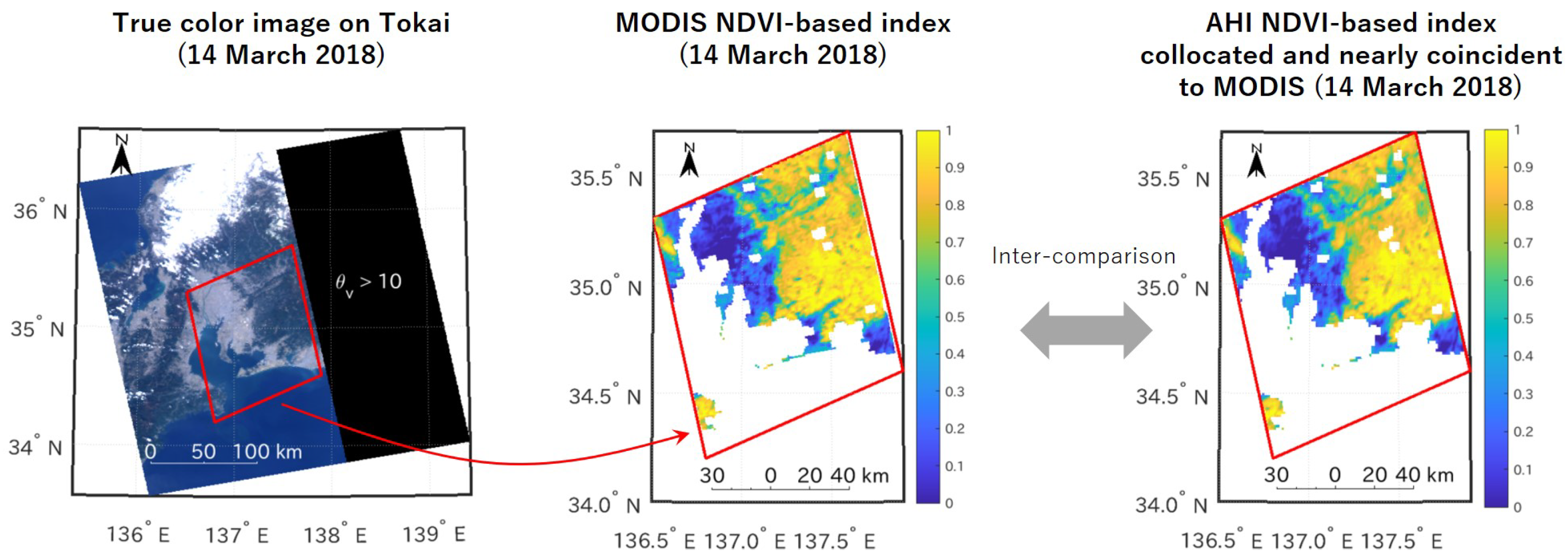
4.1. Processing Steps Used to Prepare the AHI and MODIS Scene Pairs

Pairs of nearly coincident and collocated AHI and MODIS partial scenes were prepared for the comparisons. Steps (1–4) were repeated across each region for the period between 7 July 2015 and 31 December 2018 to create pairs of MODIS and AHI data. The process flow is illustrated in Figure 4.
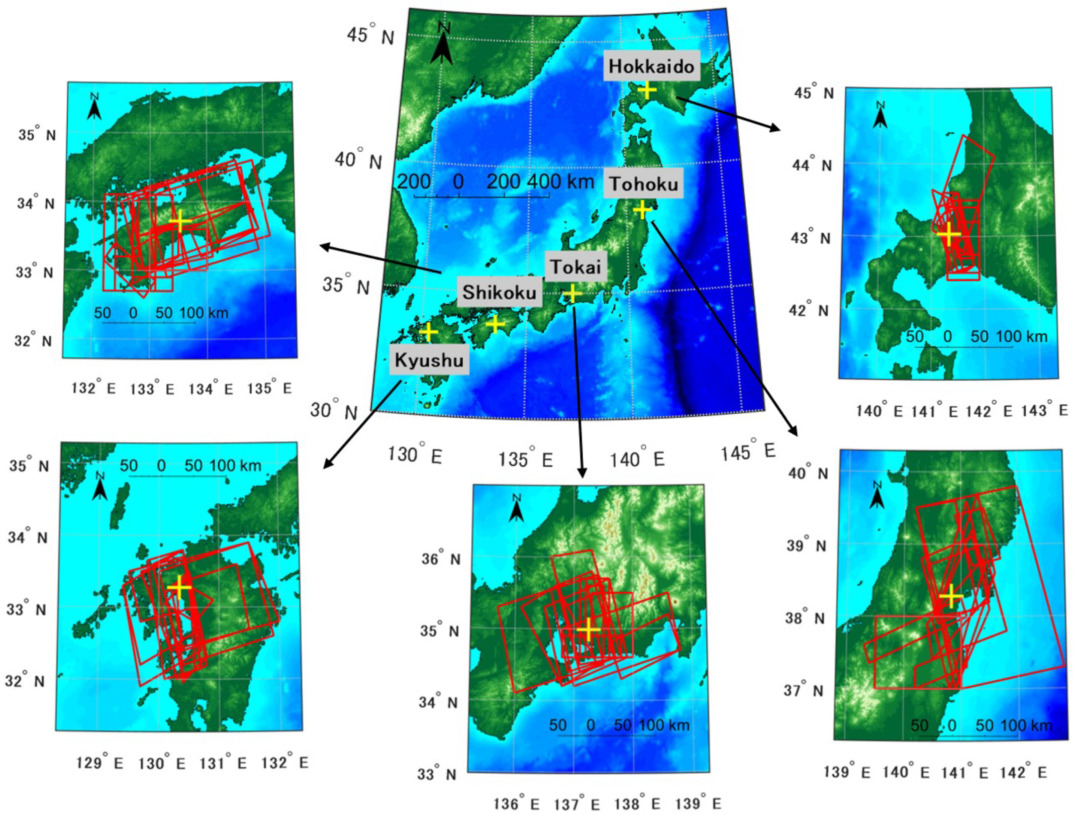
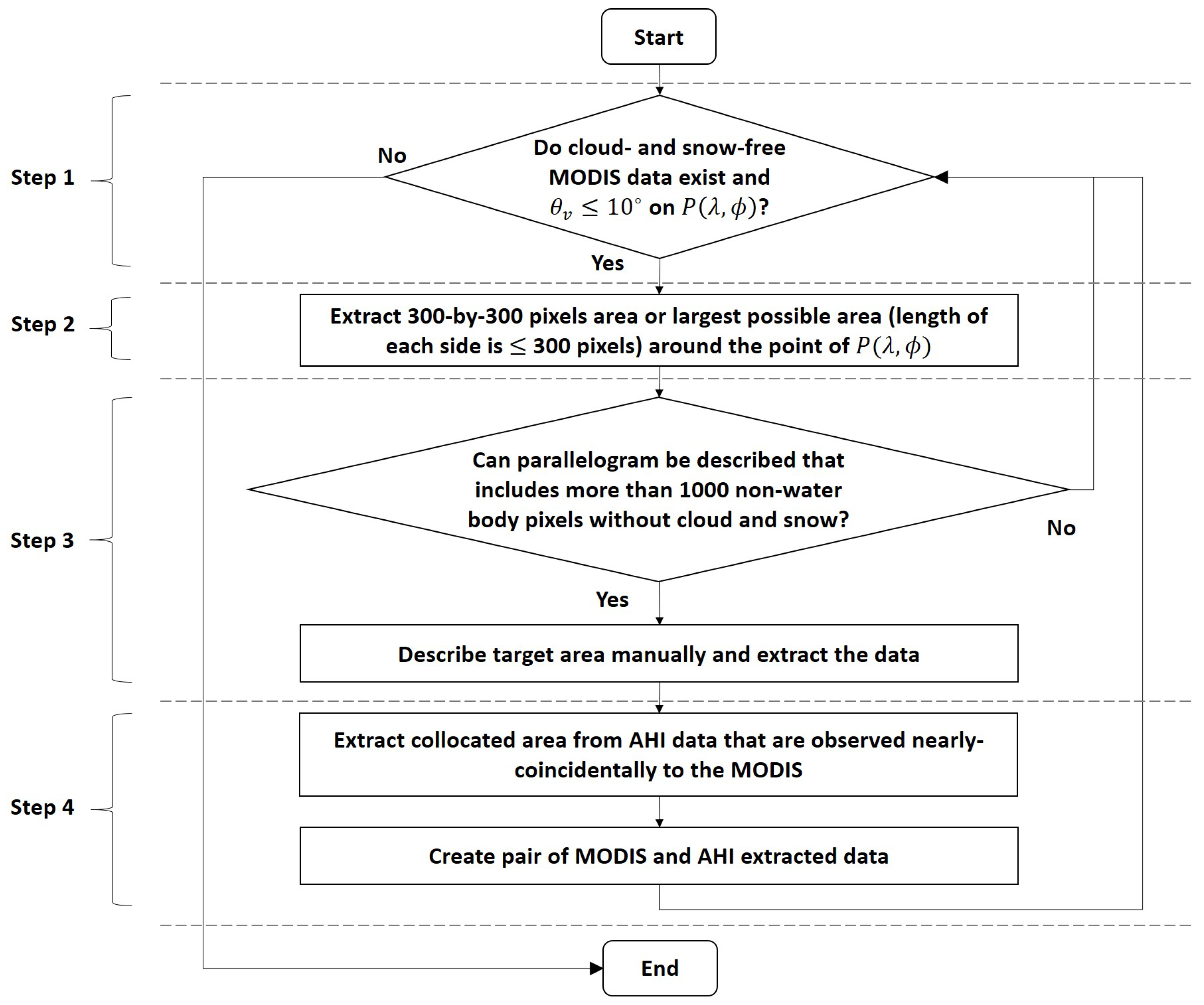
  • Search near-nadir MODIS data: MODIS scenes that included a point P ( λ i , ϕ i ) , where λ and ϕ are the latitude and longitude and i identifies the region, designated in Table 1, were explored. The scenes that satisfied the following two conditions were obtained: View zenith angle of the point ( θ v ) was equal to or less than 10 degrees, and the area around the target region was not influenced by clouds, cirrus clouds, or snow observed by visual inspection.
  • Extract an area of at most 300-by-300 km of MODIS data: If the MODIS data satisfying the above condition were found, a 300-by-300 pixel area around the center point P ( λ i , ϕ i ) or largest possible rectangular area that did not exceed 300 pixels on any side around P ( λ i , ϕ i ) was extracted. Subsequently, pixels in the data that exceeded 10 degrees of the viewing zenith angle were masked.
  • Extract a target area from the MODIS: A target area in the MODIS, selected to be as extensive as possible, was manually extracted from the 300-by-300 km data or the largest possible area of data. The shape of the area was a parallelogram that included more than 1000 non-water body pixels and did not contain cloud or snow. This was accomplished by visual inspection rather than by using cloud and snow flags, as this process almost completely avoided the effects of cloud contamination, including cirrus clouds and snow cover. The target area was selected to include water bodies, as discussed in Section 3.2.
  • Extract the AHI target area and create a scene pair: The AHI scene observed at the time closest to the MODIS observation time was selected, and the AHI partial scene corresponding to the MODIS target area was extracted to create a MODIS and AHI partial scene pair for comparison.
Figure 5 illustrates the target area extraction and NDVI-index computation for the Tokai region for 14 March 2018. The black area corresponds to the view for which the zenith angle exceeded 10 degrees (left panel in Figure 5). The NDVI-based index, computed using the algorithm introduced in Section 3 using the MODIS data on the date, is shown in the center panel in Figure 5. The NDVI-based index computed using the nearly coincident AHI data collocated to the MODIS data is shown in the right panel in Figure 5. Pixels with no data in the NDVI-based index correspond to water bodies identified by the land/sea mask in the MYD03 product.

4.2. Comparison Method

In this study, the NDVI differences between AHI and MODIS using TOA reflectances were evaluated in addition to the NDVI-based index differences. Pixels corresponding to water bodies were excluded using the land/sea mask in the MYD03 product after pseudo-endmember computation for deriving the NDVI and NDVI-based index.
Differences between the NDVI/NDVI-based indices from two sensors were evaluated using a scene-by-scene comparison by describing their relative frequency distributions, computing the differences between the average NDVI/NDVI-based indices of the AHI and MODIS, and conducting a non-parametric statistical test (Wilcoxon rank sum test) of the frequency distribution to statistically identify whether the outputs from two sensors were extracted from distributions with the same median, against the alternative that they did not, using the r a n k s u m of MATLAB®.
Pixel-by-pixel comparisons were conducted using the AHI and MODIS pairs. The effects of the lower spatial resolution of the off-nadir AHI data may have influenced the pixel-by-pixel comparison using the MODIS near-nadir data with a 1 km resolution. Uncertainties in the geometric calibration (relative geolocation errors) of the AHI and MODIS may also have impacted the comparison. The AHI and MODIS data were downscaled using the four-by-four pixel area average to mitigate the effects of the discrepancy on the actual spatial resolution and the relative geolocation errors. A nearest neighbor algorithm was then implemented to create a pixel-by-pixel pair for each AHI and MODIS pair. Coefficients of determination were computed using the results of the linear regression between the AHI (independent variable) and the MODIS (response variable) NDVI/NDVI-based indices ( R v 2 and R ω 2 for NDVI and NDVI-based indices, respectively). The variability of the differences between NDVIs can be compared with that between NDVI-based indices using the coefficients of determination. Scatter plots of the NDVI/NDVI-based index for AHI and MODIS were also shown for visually investigating the variability.

5. Results

Figure 6 shows the illumination conditions and view angles of the Tokai region for 7 July 2016 and 19 December 2015, respectively, over the polar plot. Each angle is the average value of the angles calculated on that date. Points corresponding to the solar angle for other dates are near or between the points shown in Figure 6a,b. Other regions in Japan showed similar angular conditions. The MODIS and AHI solar zenith angles (circles) differed slightly due to small differences in the observation times. During the winter, the AHI view angle was closer to the principal plane (Figure 6b) and the reflectances were sensitive to the backscattering effects that increase the reflectances. The backscattering effects were small if the solar zenith angle was small because the shadow effects decreased, especially during summer, as shown in Figure 6a.

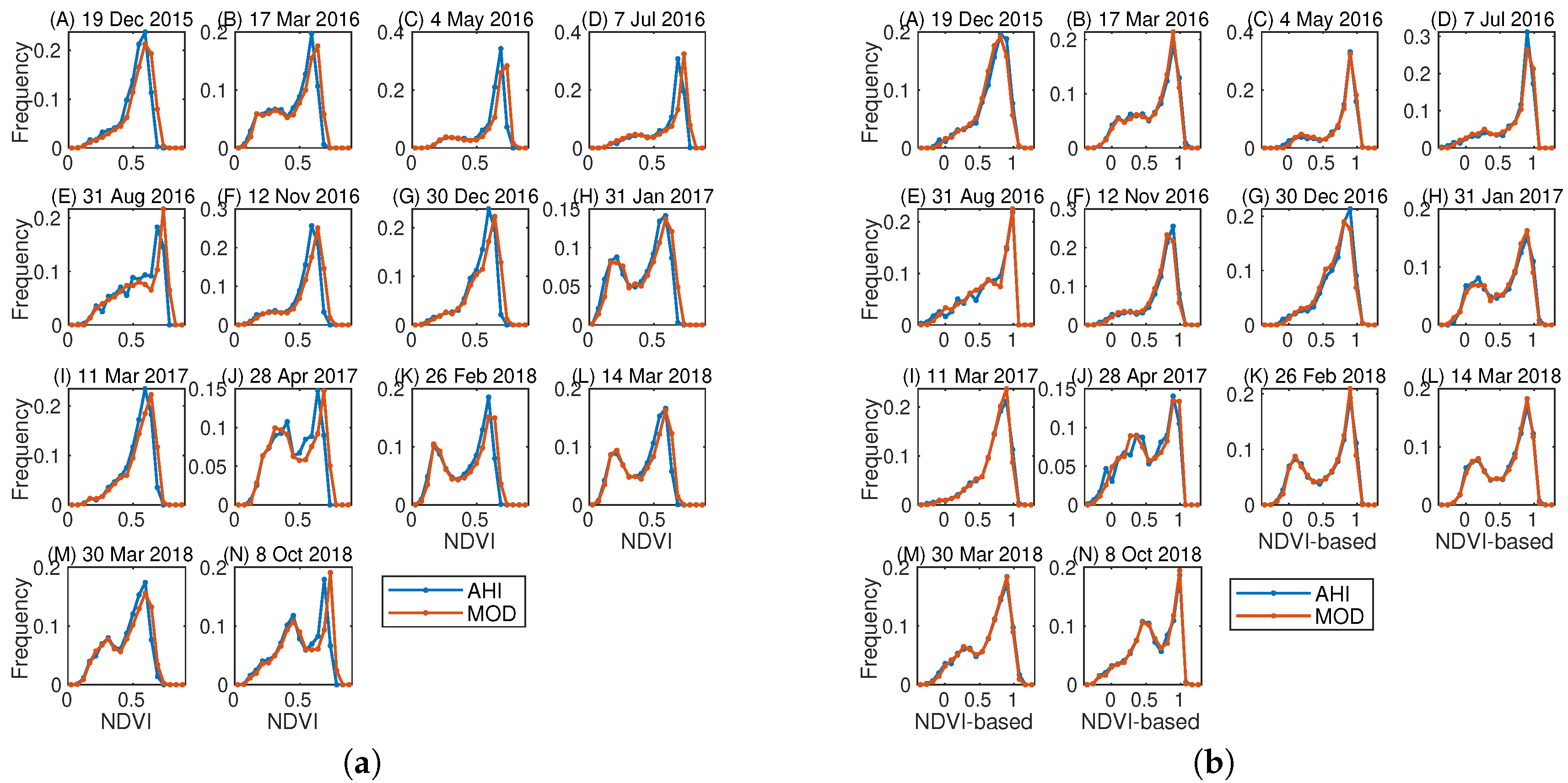
5.1. Scene-by-Scene Comparison

The relative frequency distributions of the TOA NDVI and NDVI-based indices over the Hokkaido region on 10 dates are shown in Figure 7. Data from only the spring and summer seasons could be analyzed due to the presence of snow and cloud cover in other seasons. The NDVI distribution from the AHI data differed from that of the MODIS data (Figure 7a). The MODIS NDVIs were higher than the AHI NDVIs, especially at higher NDVI values (>0.3). The distributions of the NDVI-based indices for the two sensors were more similar than the NDVI distributions (Figure 7b). The NDVI-based index could assume negative values or values exceeding 1 because the NDVI of the pseudo-vegetation endmember was lower than the maximum NDVI, or the NDVI of the pseudo-non-vegetation endmember was higher than the minimum NDVI over the area. Table 4 presents a statistical analysis of the NDVI/NDVI-based index differences. The averages of the AHI NDVI ( v ¯ a ) were 0.31–0.66 and the differences between the average NDVI ( v ¯ a minus the average MODIS NDVI), δ v , ranged from 0.036 to 0.014 . The average AHI NDVI-based index ( ω ¯ a ) was 0.44–0.65, and the magnitude of the ω ¯ a minus the average MODIS NDVI-based index, δ ω , ranged from 0.001 to 0.095.
Figure 8 shows density scatter plots of the red and NIR reflectances for the Hokkaido region on 16 July 2015, 12 August 2016, 14 July 2017, and 21 May 2018 as examples. The spectra corresponding to water bodies were excluded prior to plotting. The magnitudes of the AHI reflectances were slightly higher than those of the MODIS. Differences between the view zenith angles of the AHI and MODIS did not significantly affect the results, unlike the results observed over the Tokai region, discussed further below. The small differences effect was attributed to the fact that all dates used over the Hokkaido region fell between May and August, during which the AHI solar zenith angle average within each area was small (27–34 degrees) at 1:30 local time (the equator crossing time of Aqua). For this reason, the effects of the view zenith angle on the density scatter plots were small.
The absolute values of δ ω for 12 August 2016 and 14 July 2017 in the Hokkaido region were higher (0.0417 and 0.0945) than those for other dates (Table 4). This result was attributed to differences in reflectance density distribution between sensors. For example, Figure 8g reveals two clusters of high density in the plot of the MODIS analysis. One of the clusters was superimposed on the vegetation endmember and another assumed smaller values of the NIR reflectances (marked by an arrow in Figure 8g). Figure 8c shows that the NIR reflectances of the cluster with smaller NIR reflectances were much higher (denoted by an arrow), and the NIR reflectances of the two clusters were nearly identical. The different characteristics of the reflectance density distributions resulted in inconsistent NDVI-based index values across sensors. For example, 4.7% of the AHI NDVI-based index for 14 July 2017 was less than 0.5 while 0.2% of MODIS NDVI-based index for the date was less than 0.5 , leading to large biases in δ ω ( 0.0945 ).
The rejection of the null hypothesis ( H 0 ), which is that the outputs from the two sensors were extracted from a distribution with the same median, corresponded to 1, whereas H 0 returned 0 if the null hypothesis were not rejected. H 0 v and H 0 ω were the null hypotheses for the NDVI and NDVI-based indices. The eighth and ninth columns in Table 4 listed H 0 v and H 0 ω , respectively. H 0 v was 1 for all dates whereas H 0 ω was 0 for all dates except for 12 August 2016 and 14 July 2017.
The relative frequency distributions of the NDVI and NDVI-based indices over the Tokai region on 14 dates are shown in Figure 9. The AHI NDVI distribution was close to the MODIS distribution (Figure 9a), although slight differences were observed, especially at higher NDVI values (>0.5). The distributions of the NDVI-based indices of the two sensors were more similar than the NDVI distributions (Figure 9b). The average AHI NDVI ( v ¯ a ) was 0.41–0.59, and differences between the average NDVIs ( v ¯ a minus the average MODIS NDVI) ranged from 0.03 to 0.011 , as summarized in Table 5. The average AHI NDVI-based index ( ω ¯ a ) was 0.53–0.72 and the magnitude of the difference between the average AHI NDVI-based indices ( ω ¯ a minus the averaged MODIS NDVI-based index) were less than 0.017. The H 0 v values were equal to 1 on all dates, whereas the H 0 ω values were 0 except on four dates (19 December 2015, 4 May 2016, 12 November 2016, and 30 December 2016).
Figure 10 shows density scatter plots of the red and NIR reflectances for the Tokai region on 19 December 2015, 4 May 2016, 28 April 2017, and 8 October 2018 as examples, excluding the spectra of water bodies, over the Tokai region. The AHI reflectances were higher than the MODIS reflectances except between the months of April and August. In particular, the results for 19 December 2015 (Figure 10a,e), a date close to the winter solstice, showed large differences. The AHI NIR reflectances were 0.2–0.5 (Figure 10a) whereas the MODIS NIR reflectances were 0.1–0.3 (Figure 10e). This result was attributed to the anisotropy of the surfaces that is backscattering effects.
Statistical analyses of the differences between the AHI and MODIS NDVI as well as between the AHI and MODIS NDVI-based indices are summarized for the Tohoku, Shikoku, and Kyushu regions in Table 6, Table 7 and Table 8, respectively. Trends in the statistics were similar to those observed over the Hokkaido and Tokai regions (Table 4 and Table 5). The null hypothesis for the NDVI-based index ( H 0 ω ) over the three regions was rejected at a higher rate than in the Hokkaido and Tokai regions. Nevertheless, the number of NDVI-based index rejections was always smaller than the corresponding value for the NDVI. The δ ω computed from all ROIs was 0.0004 ± 0.018 (mean ± standard deviation) while δ v was 0.021 ± 0.007 .
The density scatter plots of Hokkaido region except for plots of four dates shown in Figure 8 are provided in Supplementary Materials (Figures S1 and S2 for AHI and MODIS), and the plots of the Tokai region except for plots of four dates shown in Figure 10 are provided in Supplementary Materials (Figures S3 and S4 for AHI and MODIS). In addition, histograms of the relative frequency distributions of the NDVI and NDVI-based indices and the density scatter plots of the AHI and MODIS for Tohoku, Shikoku, and Kyushu regions are provided in Supplementary Materials (Figures S5–S16).

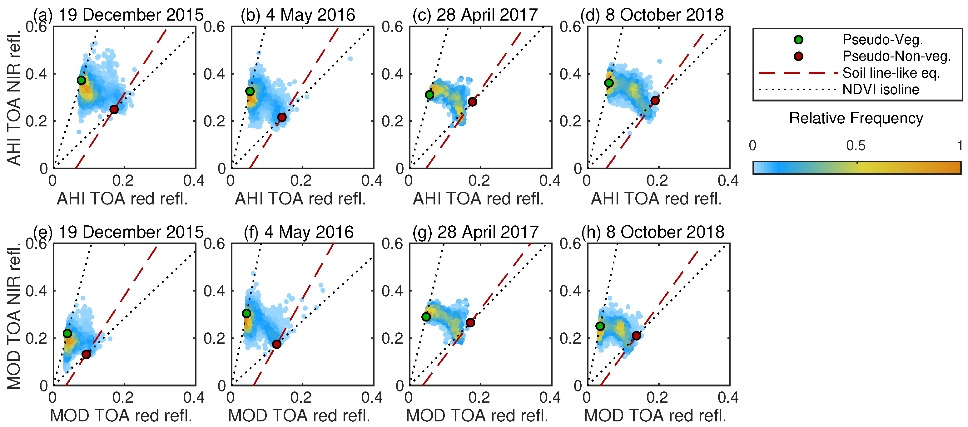
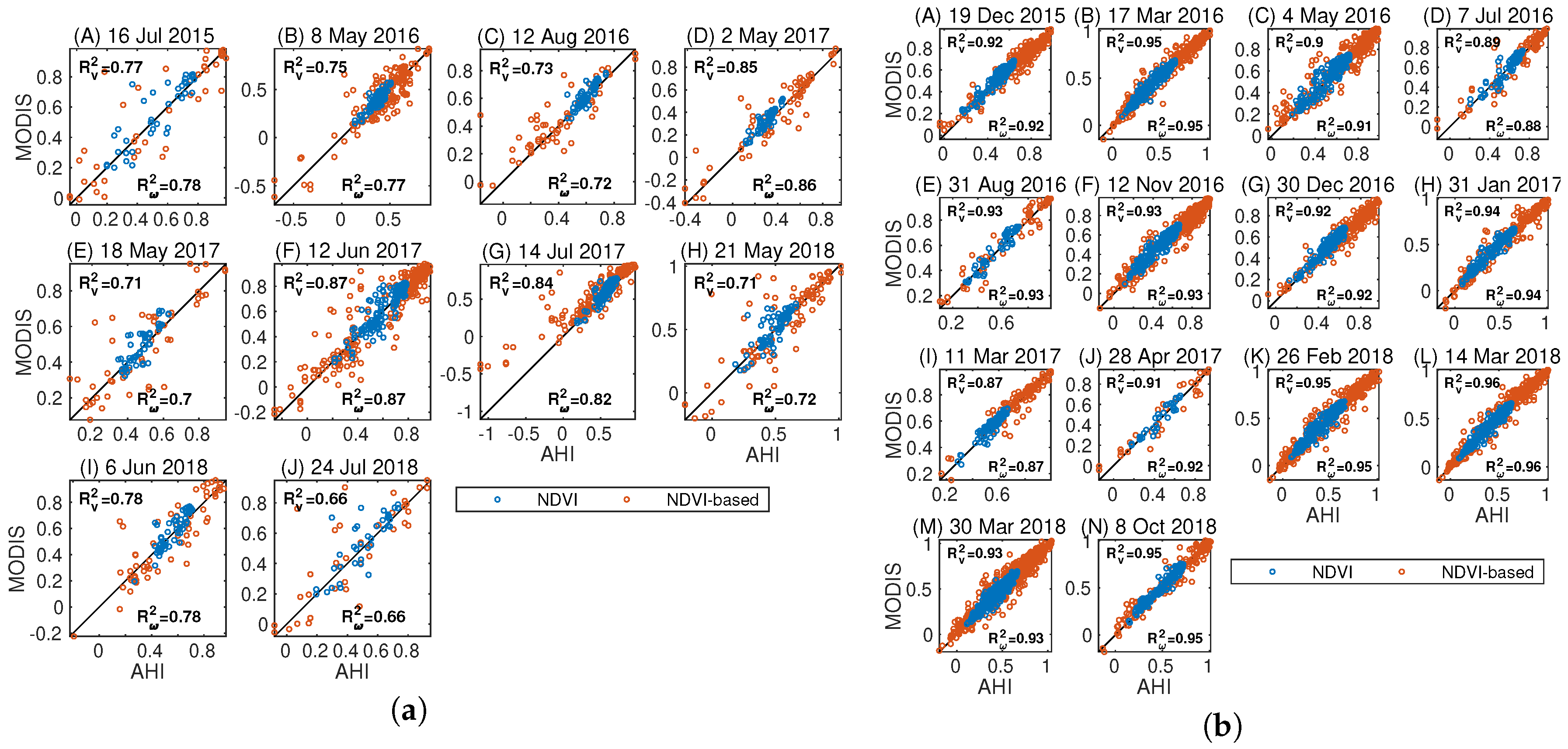
5.2. Pixel-by-Pixel Comparison

The variability of NDVI/NDVI-based index differences was evaluated by the pixel-by-pixel comparison using downscaled AHI and MODIS reflectance pairs. The NDVI between-sensor coefficients of determination, R v 2 , and the corresponding NDVI-based coefficients, R ω 2 , were computed on each date and within each region, as summarized in the right-most two columns in Table 4, Table 5, Table 6, Table 7 and Table 8. The values of R v 2 and R ω 2 were comparable on each date within each region. The values of the coefficients depended on the region, scene, and number of pixels included in each area. Figure 11 shows the scatter plots of the MODIS vs. AHI NDVIs and MODIS vs. AHI NDVI-based indices for the Hokkaido region (Figure 11a) and the Tokai region (Figure 11b). The results indicate that the variability of NDVI-based index differences was comparable to that of the NDVI differences while biases between NDVI-based indices of sensors were mitigated by using the developed algorithm, as shown in previous subsection.

6. Discussion

6.1. Differences between the Sensor-Specific NDVI/NDVI-Based Indices

The AHI NDVI calculated using the TOA reflectances (40–50 degree view zenith) displayed a negative bias (about 0.02) relative to the near-nadir MODIS TOA NDVI. The differences between the NDVIs were characterized using a scatter plot of the AHI and MODIS reflectances. Figure 12a shows the AHI and MODIS reflectances (blue and red dots) used in pixel-by-pixel comparisons over the Tokai region on 8 October 2018. The gray line revealed the trajectory of the reflectance change between the AHI and MODIS. The change of spectrum resulted primarily from surface anisotropy, but the SRF effects also contributed. The slope of the trajectory line was smaller when the red and NIR reflectances were similar; that is, the NDVI values were small. The slope gradually increased as the red reflectances decreased (increasing NDVI). The trajectory line slope resembled the NDVI isoline described by the dotted lines in Figure 12a, suggesting that in this case, the NDVI mitigated the effects of the sensor dependencies. The magnitude of δ v on this date was not large (0.024); however, the trajectories did not necessarily match the NDVI isoline on other dates or in other regions. Figure 12b shows an additional example over the Hokkaido region for 12 Jun 2017. The trajectory of the reflectance change differed from the NDVI isoline, for example, in areas with medium vegetation corresponding to the two ellipsoids in Figure 12b. In this area, the MODIS spectra (magenta ellipsoid) shifted almost vertically into the AHI spectra (cyan ellipsoid). Effects of relative geolocation errors manifested as anomalous trajectories. The errors in these trajectories may have been caused by geolocation errors in AHI data from the NICT showing temporal variations [62]. Geolocation errors of Aqua MODIS, by contrast, have been reported to be less than 60 m [63]. Although the NDVI might have mitigated the anisotropy effects, the SRF effects biased the NDVIs calculated by the two sets of sensors.
The NDVI-based index computed by the algorithm developed here further mitigated the effects of the sensor dependencies. The value of the NDVI-based index is determined at the intersection of the NDVI isoline and the subspace of pseudo-endmember spectra described by yellow lines in Figure 12a,b [36]; hence, the geometric relationship between the target spectra and the simulated endmember spectra for AHI should be similar to those calculated for the MODIS data. Figure 12a shows that the geometric relationship between target and pseudo-endmember spectra for AHI is indeed similar to those for MODIS. In addition, the gradual increase in the slope of the trajectory lines (gray lines in Figure 12a) with the proper endmember spectra indicates that the NDVI-based index is similar across sensors even though the view zenith angles are different. This implies that vegetation in each pixel was likely spatially segregated. The magnitude of δ ω on a particular date was small (0.009). Caution should be taken when interpreting areas with medium vegetation (the actual FVC likely spanned 0.2–0.8), within which dramatic increases in the NIR bands were identified at larger viewing zenith angles (Figure 12b), as discussed above. The distance between the AHI target spectra (cyan ellipsoid) and the AHI pseudo-non-vegetation endmember (red filled circle) was larger than the corresponding MODIS distance (magenta ellipsoid and brown filled circles), which increased the AHI NDVI-based index relative to the MODIS index. Similar trends in the reflectance shift were identified at other ROIs in the Hokkaido region (e.g., Figure 8c,g), resulting in lower AHI NDVI-based index values, especially in pixels with a low NDVI-based index (< 0.5 ), as discussed in the previous section.
The relatively large increase in the NIR reflectances likely stemmed from changes in the directional fraction of the vegetation cover. Intuitively, visible soil surface areas between the canopies are expected to decrease at large view zenith angles [38], especially in areas that include, for example, scattered trees over artificial materials with 50% tree cover. The increases in the directional fraction of vegetation cover should increase the top-of-canopy NIR reflectances. This situation may have been present in several pixels. This work did not seek to correct this effect.
The characteristic differences between the NDVI-based sensor indices provided important information about where the LMM assumption could be applied and where the NDVI-based index, i.e., the FVC-like index from AHI was sufficiently consistent with the index based on the near-nadir MODIS data, within a certain uncertainty.

6.2. Comparison with Previous Studies

To the best of our knowledge, only a few studies have discussed differences in FVC data obtained using GEO and LEO sensors. A key work on this topic was a series of studies on the MSG SEVIRI FVC data products [7], which determine FVC using an algorithm based on the stochastic spectral mixture model. In that series of studies, the MSG SEVIRI FVC data were compared with those of LEO’s FVC products, with SPOT VEGETATION data as a reference [7]. The SPOT FVC was based on a neural network that was trained to generate the best estimates of LAI, fraction of absorbed photosynthetically active radiation (FAPAR), and FVC from the fused and scaled MODIS and Carbon Cycle and Change in Land Observational Products from an Ensemble of Satellites (CYCLOPES) products [64]. Although the MSG SEVIRI and SPOT VEGETATION approaches yielded consistent results of FVC for a site in Gabon (Figure 11 in [7]), the algorithms implemented to retrieve FVC were not identical. Our intention in the present work was to compare FVCs (NDVI-based indices in this study) obtained using GEO and LEO sensors with an identical algorithm. Thus, the results of our study shed light on possible discrepancies in FVCs between the GEO and LEO sensors caused by the differences in geometric conditions and sensor specifications.
Most comparisons of data from GEO and LEO sensors have examined differences in reflectances and spectral vegetation indices such as the NDVI as representative parameters. Some of them performed corrections for atmospheric influences and BRDF effects [18,22,23,24,65]. Those studies reported biases in NDVI. For example, the AHI NDVI computed from reflectances after atmospheric and BRDF correction was higher than the MODIS NDVI (the 16-day MODIS composite product (MOD13A2)) [18]. By contrast, the TOA MODIS NDVI was somewhat higher than the TOA AHI NDVI in this study. This discrepancy may be due to differences in correction levels and the test site. Specifically, uncorrected TOA reflectances were used in this study whereas corrected reflectances were used in previous works. Further studies are needed to investigate this issue.
In another study comparing NDVI data in the GEO-LEO framework, SEVIRI NDVI (atmospherically and BRDF-corrected) and MODIS NDVI based on the MCD43A4 16-day Nadir BRDF-Adjusted Reflectance (NBAR) product were compared [22]. The study found differences in NDVI between the two systems, which were attributed to sensor-dependent variations in the accuracies of the BRDF corrections as well as differences in SRF. In another study, NDVI data obtained from atmospherically corrected and BRDF-adjusted reflectances recorded by the Geostationary Ocean Colour Imager (GOCI) on the Korean Communication, Ocean and Meteorological Satellite (COMS) were compared with MODIS [23,65]. It should be noted that GOCI data used in the comparisons included the reflectance standardized to GOCI’s own fixed view angle with the mean solar zenith angle [65]. Unlike the NBAR products, the view zenith angle was not adjusted to the nadir direction. The GOCI NDVI was compared with the MODIS NDVI computed from the nadir BRDF-adjusted reflectances provided by the BRDF model based on the RTLSR kernels that had been calibrated using a surface reflectance product (MOD09GA and MYD09GA) [65]. The study showed that the GOCI NDVI was lower than MODIS NDVI, with differences in the SRF being the suspected major cause of systematic errors in NDVI [23,65].
In general, inconsistencies between GEO and LEO NDVI values derive from differences in SRFs. In addition, uncertainties in the BRDF model (and its inversion process) also influence the accuracy of the BRDF correction. Moreover, such uncertainties are strongly influenced by the quality of the data, which can be degraded by cloud contamination, atmospheric effects, and/or poor scene geometry [22]. The algorithm developed in this study does not employ a BRDF model. For this reason, use of the proposed algorithm may reduce systematic errors between GEO and LEO vegetation products caused by BRDF and SRF effects.

6.3. Characteristics in the Developed Algorithm

The NDVI-based index for the BOA as a function of the TOA reflectances was approximated using the radiative transfer theory. The atmospheric model was homogeneous over the entire area of the single partial scene. Actual data were not homogeneous. The Rayleigh scattering depended on the atmospheric pressure specific to the elevation, and the aerosol loading and water vapor content were heterogeneous in the spatial domain. These effects may have added errors to the NDVI-based index [66]. The atmospheric effects required correction to mitigate the effects of the atmospheric heterogeneity in the subsequent comparison steps.
Significantly, training data, ancillary data, or statistical functions may not be required to obtain the view zenith angle- and SRF (sensor)-independent NDVI-based indices for areas where the LMM assumption can be applied in the context of the synergistic use of GEO and LEO sensors. It means that regression analysis is not required to obtain indices compatible between sensors. It is also important to note that the NDVI-based index was less sensitive to calibration uncertainties because the endmember spectra simulated using the algorithm developed here and the target spectra were both influenced by uncertainties, meaning that systematic components of the uncertainties in the endmember and target spectra canceled one another. This point should be further investigated.
The NDVI-based indices independently estimated from different locations could not be directly compared because the simulated endmember spectra were scene-dependent; however, small differences between the NDVI-based indices without external data would be beneficial for the development of algorithms for the inter-sensor translation of the NDVI. The NDVI-based index may be a parameter for relating vegetation indices of a reference sensor and a destination senor. Previously, soil brightness was used as a parameter to derive the inter-sensor relationships between vegetation indices [67], and the soil isoline equations were used to relate the vegetation indices [68]. Small differences between the NDVI-based AHI and MODIS indices thus demonstrated the applicability of the developed algorithm and suggested that the vegetation indices might be translated between sensors using the NDVI-based index as a parameter for GEO-LEO and/or LEO-LEO data fusion.

7. Conclusions

This study developed an algorithm for deriving the NDVI-based index that was designed to be compatible between GEO and LEO sensors. In the inter-comparison results, the NDVI-based indices calculated from AHI off-nadir observations (40–50 degree viewing zenith angles) were, in general, compatible with the MODIS near-nadir observations made in mid-latitude (Japanese) areas in which the vegetation in a pixel might have been spatially segregated, and the fractional abundances of each component were less sensitive to the view zenith angle. The algorithm developed here to automatically compute the pseudo-vegetation and non-vegetation endmember spectra mitigated the sensor dependencies, including the effects of differences between the viewing geometries and the sensor’s SRFs over the areas. By contrast, the NDVI-based indices showed large biases in some areas. This effect can be attributed to the effects of sparsely scattered vegetation (e.g., scattered trees) within individual pixels. The directional fractions of vegetation canopy in such areas increased with increasing view zenith angle.
The NDVI-based index computed using the algorithm developed here showed better consistency in the relative frequencies relative to the TOA NDVI. In this study, the AHI TOA NDVIs displayed a negative bias relative to the MODIS TOA NDVIs (about 0.02) due to sensor dependencies.
The inter-comparison and integration of GEO and LEO data have been hindered by BRDF and SRF effects. As shown in several studies, one way to minimize these biases is to perform BRDF correction. However, this approach has the drawback that it requires prior knowledge of the BRDF model for each target. The accuracy with which the output of one sensor can be transformed to that of another sensor depends largely on the accuracy of the BRDF model. Moreover, minimization of the effects of differences in SRFs between the two sensors often requires statistical methods such as regression analysis. In general, the set of coefficients determined by the regression varies significantly according to land cover type. Furthermore, the coefficients are specific to each sensor pair. On the contrary, the algorithm developed in this study can derive comparable NDVI-based indices for GEO and LEO sensors without using regression analysis (training data). Because this novel approach does not require regressions between the two sensors, it has advantages over existing methods in which the set of coefficients determined by the regression depends on land cover type and the sensor pair.
The characteristics of the NDVI-based index differences over other areas, in the presence of atmospherically corrected reflectances, should be further investigated. Such studies will explore the applicability of fusing NDVI-based indices from GEO and LEO sensors. At least small biases in the NDVI-based indices calculated from different sensors over certain areas encourage the use of GEO sensors to complement LEO observations and the inter-sensor translation of vegetation indices for monitoring terrestrial vegetation.

Supplementary Materials

The following are available online at https://www.mdpi.com/2072-4292/12/15/2417/s1, Tables S1–S5: Latitude (°N) and longitude (°E) for areas demarcated with parallelograms on each date in the Hokkaido, Tohoku, Tokai, Shikoku, and Kyushu regions. Figures S1–S4: Density scatter plots of the AHI and MODIS reflectances for the Hokkaido and Tokai regions that are not shown in Figure 8 and Figure 10. Figures S5–S16: Histograms of the relative frequency distributions of the NDVI and NDVI-based indices and density scatter plots of the AHI and MODIS reflectances for the Tohoku, Shikoku, and Kyushu regions.

Author Contributions

Conceptualization, K.O.; methodology, K.O.; software, K.O.; validation, K.O., H.Y.; formal analysis, K.O.; investigation, K.O. and H.Y.; resources, K.O.; data curation, K.O.; writing—original draft preparation, K.O.; writing—review and editing, K.O. and H.Y.; visualization, K.O; project administration, K.O. and H.Y.; funding acquisition, K.O. and H.Y. All authors have read and agreed to the published version of the manuscript.

Funding

This research was supported by the Hibi Science Foundation (KO) and the JSPS KAKENHI Grant number 20K12259 (KO), 19H05583, 20K20487 (HY), and 17K07843 (HY).

Acknowledgments

AHI data were downloaded from the NICT science cloud. MODIS land cover data (MCD12Q1C) and Aqua MODIS calibrated radiances (MYD021KM) and their geolocation data (MYD03) were downloaded from the LAADS DAAC. The GMTED2010 data with spatial resolution of 30 arc-seconds were downloaded from EarthExplorer. Map services and data for the SRTM30 Plus are available from the NASA WorldWind WMS.

Conflicts of Interest

The authors declare no conflicts of interest. The funders had no role in the design of the study, in the collection, analysis, or interpretation of data, in the writing of the manuscript, or in the decision to publish the results.

Abbreviations

The following abbreviations are used in this manuscript:
GEOGeostationary
LEOLow earth orbit
SRFSpectral response function
NDVINormalized Difference Vegetation Index
LMMLinear mixture model
FVCFraction of vegetation cover
AHIAdvanced Himawari Imager
MODISModerate Resolution Imaging Spectroradiometer
MSGMeteosat Second Generation
SEVIRISpinning Enhanced Visible and Infrared Imager
BRDFBidirectional Reflectance Distribution Function
GOCIGeostationary Ocean Color Imager
TOATop-of-atmosphere
BOABottom-of-atmosphere
ROIRegion of interest
IGBPInternational Geosphere-Biosphere Programme
SAVISoil Adjusted Vegetation Index

Appendix A. Approximation of the FVC Using the TOA Reflectances

All spectral variables here depended on the sun–target–sensor viewing geometry; angular variables were omitted here for brevity. TOA reflectances, ρ ^ b a n d a t m , are modeled by
ρ ^ b a n d a t m = ρ a , b a n d + T b a n d T b a n d [ ω ρ v , b a n d + ( 1 ω ) ρ s , b a n d ] + o b a n d ,
where ρ a , b a n d is the atmospheric path radiance, T b a n d and T b a n d are the downward and upward atmospheric transmittances, and o b a n d is the reflectance corresponding to the second- and higher-order interaction terms between the atmosphere and surface modeled by the LMM,
o b a n d = T b a n d T b a n d S b a n d [ ω ρ v , b a n d + ( 1 ω ) ρ s , b a n d ] 2 1 S b a n d [ ω ρ v , b a n d + ( 1 ω ) ρ s , b a n d ] ,
and S b a n d is the spherical albedo of the atmosphere. This expression is often used to model TOA reflectances (e.g., [69,70]).
The NDVI computed using the TOA reflectances over the target ( ρ b a n d a t m ) was assumed to be equal to the NDVI computed from the modeled TOA reflectances (Equation (A1)),
v a t m = v ^ a t m ,
where
v a t m = ρ n a t m ρ r a t m ρ n a t m + ρ r a t m ,
v ^ a t m = ρ ^ n a t m ρ ^ r a t m ρ ^ n a t m + ρ ^ r a t m .
Here, o b a n d in Equation (A2) was assumed to remain constant, although it is a function of ω . ω could be derived by substituting Equation (A1) into Equation (A3),
ω = f 1 ( v a t m , ρ s a t m ) + ϵ 1 f 2 ( v a t m , ρ v a t m , ρ s a t m ) + ϵ 2 ,
where ρ e m a t m = [ ρ e m , r a t m , ρ e m , n a t m ] and ϵ 1 and ϵ 2 are functions of the higher-order interaction terms,
ρ e m , b a n d a t m = ρ a , b a n d + T b a n d T b a n d ρ e m , b a n d + o e m , b a n d ,
ϵ 1 = o n o r o s , n + o s , r v a t m ( o n + o r o s , n o s , r ) ,
ϵ 2 = o v , n o v , r o s , n + o s , r v a t m ( o v , n + o v , r o s , n o s , r )
and
o e m , b a n d = T b a n d T b a n d S b a n d ρ e m , b a n d 2 1 S b a n d ρ e m , b a n d ,
where o e m , b a n d is the reflectance of the second- and higher-order interaction terms between the atmosphere and surface. Equation (A10) describing the vegetation endmember was equal to Equation (A2) if ω = 1 , and Equation (A10) for the non-vegetation endmember was equal to Equation (A2) if ω = 0 .
The values of ϵ i ( i = 1 , 2 ) in Equation (A6) were expected to be small because the terms of each band (e.g., o n and o s , n in Equation (A7)) canceled out their values if the values of the second- and higher-order interaction terms were comparable. Assuming that ϵ i in Equation (A6) was equal to zero, ω could be represented as follows:
ω f 1 ( v a t m , ρ s a t m ) f 2 ( v a t m , ρ v a t m , ρ s a t m ) .
Numerical simulations to evaluate and validate these approximations may be presented in a separate study.

References

  1. Zhang, Y.; Song, C.; Band, L.E.; Sun, G.; Li, J. Reanalysis of global terrestrial vegetation trends from MODIS products: Browning or greening? Remote Sens. Environ. 2017, 191, 145–155. [Google Scholar] [CrossRef]
  2. Sexton, J.O.; Song, X.P.; Huang, C.; Channan, S.; Baker, M.E.; Townshend, J.R. Urban growth of the Washington, D.C.–Baltimore, MD metropolitan region from 1984 to 2010 by annual, Landsat-based estimates of impervious cover. Remote Sens. Environ. 2013, 129, 42–53. [Google Scholar] [CrossRef]
  3. Claessen, J.; Molini, A.; Martens, B.; Detto, M.; Demuzere, M.; Miralles, D.G. Global biosphere–climate interaction: A causal appraisal of observations and models over multiple temporal scales. Biogeosciences 2019, 16, 4851–4874. [Google Scholar] [CrossRef]
  4. Fensholt, R.; Sandholt, I.; Stisen, S.; Tucker, C. Analysing NDVI for the African continent using the geostationary meteosat second generation SEVIRI sensor. Remote Sens. Environ. 2006, 101, 212–229. [Google Scholar] [CrossRef]
  5. Guan, K.; Medvigy, D.; Wood, E.F.; Caylor, K.K.; Li, S.; Jeong, S. Deriving Vegetation Phenological Time and Trajectory Information Over Africa Using SEVIRI Daily LAI. IEEE Trans. Geosci. Remote Sens. 2014, 52, 1113–1130. [Google Scholar] [CrossRef]
  6. Barbosa, H.A.; Lakshmi Kumar, T.; Paredes, F.; Elliott, S.; Ayuga, J. Assessment of Caatinga response to drought using Meteosat-SEVIRI Normalized Difference Vegetation Index (2008–2016). ISPRS J. Photogramm. Remote Sens. 2019, 148, 235–252. [Google Scholar] [CrossRef]
  7. García-Haro, F.J.; Camacho, F.; Martínez, B.; Campos-Taberner, M.; Fuster, B.; Sánchez-Zapero, J.; Gilabert, M.A. Climate Data Records of Vegetation Variables from Geostationary SEVIRI/MSG Data: Products, Algorithms and Applications. Remote Sens. 2019, 11, 2103. [Google Scholar] [CrossRef]
  8. Bessho, K.; Date, K.; Hayashi, M.; Ikeda, A.; Imai, T.; Inoue, H.; Kumagai, Y.; Miyakawa, T.; Murata, H.; Ohno, T.; et al. An Introduction to Himawari-8/9 Japan’s New-Generation Geostationary Meteorological Satellites. J. Meteorol. Soc. Japan Ser. II 2016, 94, 151–183. [Google Scholar] [CrossRef]
  9. Schmit, T.J.; Griffith, P.; Gunshor, M.M.; Daniels, J.M.; Goodman, S.J.; Lebair, W.J. A Closer Look at the ABI on the GOES-R Series. Bull. Am. Meteorol. Soc. 2017, 98, 681–698. [Google Scholar] [CrossRef]
  10. Yang, J.; Zhang, Z.; Wei, C.; Lu, F.; Guo, Q. Introducing the New Generation of Chinese Geostationary Weather Satellites, Fengyun-4. Bull. Am. Meteorol. Soc. 2017, 98, 1637–1658. [Google Scholar] [CrossRef]
  11. EUMETSAT. METEOSAT Third Generation. Available online: https://www.eumetsat.int/website/home/Satellites/FutureSatellites/MeteosatThirdGeneration/index.html (accessed on 13 February 2020).
  12. Miura, T.; Nagai, S.; Takeuchi, M.; Ichii, K.; Yoshioka, H. Improved Characterisation of Vegetation and Land Surface Seasonal Dynamics in Central Japan with Himawari-8 Hypertemporal Data. Sci. Rep. 2019, 9, 15692. [Google Scholar] [CrossRef] [PubMed]
  13. Ma, X.; Huete, A.; Tran, N.N.; Bi, J.; Gao, S.; Zeng, Y. Sun-Angle Effects on Remote-Sensing Phenology Observed and Modelled Using Himawari-8. Remote Sens. 2020, 12, 1339. [Google Scholar] [CrossRef]
  14. Chen, Y.; Sun, K.; Chen, C.; Bai, T.; Park, T.; Wang, W.; Nemani, R.R.; Myneni, R.B. Generation and Evaluation of LAI and FPAR Products from Himawari-8 Advanced Himawari Imager (AHI) Data. Remote Sens. 2019, 11, 1517. [Google Scholar] [CrossRef]
  15. Li, S.; Wang, W.; Hashimoto, H.; Xiong, J.; Vandal, T.; Yao, J.; Qian, L.; Ichii, K.; Lyapustin, A.; Wang, Y.; et al. First Provisional Land Surface Reflectance Product from Geostationary Satellite Himawari-8 AHI. Remote Sens. 2019, 11, 2990. [Google Scholar] [CrossRef]
  16. He, T.; Zhang, Y.; Liang, S.; Yu, Y.; Wang, D. Developing Land Surface Directional Reflectance and Albedo Products from Geostationary GOES-R and Himawari Data: Theoretical Basis, Operational Implementation, and Validation. Remote Sens. 2019, 11, 2655. [Google Scholar] [CrossRef]
  17. Wang, W.; Li, S.; Hashimoto, H.; Takenaka, H.; Higuchi, A.; Kalluri, S.; Nemani, R. An Introduction to the Geostationary-NASA Earth Exchange (GeoNEX) Products: 1. Top-of-Atmosphere Reflectance and Brightness Temperature. Remote Sens. 2020, 12, 1267. [Google Scholar] [CrossRef]
  18. Seong, N.H.; Jung, D.; Kim, J.; Han, K.S. Evaluation of NDVI Estimation Considering Atmospheric and BRDF Correction through Himawari-8/AHI. Asia-Pac. J. Atmos. Sci. 2020, 56, 265–274. [Google Scholar] [CrossRef]
  19. Klein, C.; Bliefernicht, J.; Heinzeller, D.; Gessner, U.; Klein, I.; Kunstmann, H. Feedback of observed interannual vegetation change: A regional climate model analysis for the West African monsoon. Clym. Dyn. 2017, 48, 2837–2858. [Google Scholar] [CrossRef]
  20. Adachi, Y.; Kikuchi, R.; Obata, K.; Yoshioka, H. Relative Azimuthal-Angle Matching (RAM): A Screening Method for GEO-LEO Reflectance Comparison in Middle Latitude Forests. Remote Sens. 2019, 11, 1095. [Google Scholar] [CrossRef]
  21. Fensholt, R.; Sandholt, I.; Proud, S.R.; Stisen, S.; Rasmussen, M.O. Assessment of MODIS sun-sensor geometry variations effect on observed NDVI using MSG SEVIRI geostationary data. Int. J. Remote Sens. 2010, 31, 6163–6187. [Google Scholar] [CrossRef]
  22. Proud, S.R.; Zhang, Q.; Schaaf, C.; Fensholt, R.; Rasmussen, M.O.; Shisanya, C.; Mutero, W.; Mbow, C.; Anyamba, A.; Pak, E.; et al. The Normalization of Surface Anisotropy Effects Present in SEVIRI Reflectances by Using the MODIS BRDF Method. IEEE Trans. Geosci. Remote Sens. 2014, 52, 6026–6039. [Google Scholar] [CrossRef]
  23. Yeom, J.M.; Kim, H.O. Comparison of NDVIs from GOCI and MODIS Data towards Improved Assessment of Crop Temporal Dynamics in the Case of Paddy Rice. Remote Sens. 2015, 7, 11326–11343. [Google Scholar] [CrossRef]
  24. Yeom, J.M.; Jeong, S.; Jeong, G.; Ng, C.T.; Deo, R.C.; Ko, J. Monitoring paddy productivity in North Korea employing geostationary satellite images integrated with GRAMI-rice model. Sci. Rep. 2018, 8, 16121. [Google Scholar] [CrossRef] [PubMed]
  25. Yan, D.; Zhang, X.; Nagai, S.; Yu, Y.; Akitsu, T.; Nasahara, K.N.; Ide, R.; Maeda, T. Evaluating land surface phenology from the Advanced Himawari Imager using observations from MODIS and the Phenological Eyes Network. Int. J. Appl. Earth Obs. Geoinf. 2019, 79, 71–83. [Google Scholar] [CrossRef]
  26. Wanner, W.; Li, X.; Strahler, A.H. On the derivation of kernels for kernel-driven models of bidirectional reflectance. J. Geophys. Res. Atmos. 1995, 100, 21077–21089. [Google Scholar] [CrossRef]
  27. Schaaf, C.B.; Gao, F.; Strahler, A.H.; Lucht, W.; Li, X.; Tsang, T.; Strugnell, N.C.; Zhang, X.; Jin, Y.; Muller, J.P.; et al. First operational BRDF, albedo nadir reflectance products from MODIS. Remote Sens. Environ. 2002, 83, 135–148. [Google Scholar] [CrossRef]
  28. Trishchenko, A.P.; Cihlar, J.; Li, Z. Effects of spectral response function on surface reflectance and NDVI measured with moderate resolution satellite sensors. Remote Sens. Environ. 2002, 81, 1–18. [Google Scholar] [CrossRef]
  29. Trishchenko, A.P. Effects of spectral response function on surface reflectance and NDVI measured with moderate resolution satellite sensors: Extension to AVHRR NOAA-17, 18 and METOP-A. Remote Sens. Environ. 2009, 113, 335–341. [Google Scholar] [CrossRef]
  30. Qin, Y.; McVicar, T.R. Spectral band unification and inter-calibration of Himawari AHI with MODIS and VIIRS: Constructing virtual dual-view remote sensors from geostationary and low-Earth-orbiting sensors. Remote Sens. Environ. 2018, 209, 540–550. [Google Scholar] [CrossRef]
  31. Fan, X.; Liu, Y. Multisensor Normalized Difference Vegetation Index Intercalibration: A Comprehensive Overview of the Causes of and Solutions for Multisensor Differences. IEEE Geosci. Remote Sens. Mag. 2018, 6, 23–45. [Google Scholar] [CrossRef]
  32. Gao, L.; Wang, X.; Johnson, B.A.; Tian, Q.; Wang, Y.; Verrelst, J.; Mu, X.; Gu, X. Remote sensing algorithms for estimation of fractional vegetation cover using pure vegetation index values: A review. ISPRS J. Photogramm. Remote Sens. 2020, 159, 364–377. [Google Scholar] [CrossRef]
  33. Adams, J.B.; Smith, M.O.; Johnson, P.E. Spectral mixture modeling: A new analysis of rock and soil types at the Viking Lander 1 Site. J. Geophys. Res. Solid Earth Planets 1986, 91, 8098–8112. [Google Scholar] [CrossRef]
  34. Verstraete, M.; Pinty, B. The potential contribution of satellite remote-sensing to the understanding of arid lands processes. In Vegetation and Climate Interactions in Semi-Arid Regions; Henderson-Sellers, A., Pitman, A., Eds.; Springer: Dordrecht, The Netherlands, 1991; pp. 59–72. [Google Scholar]
  35. Wittich, K.P.; Hansing, O. Area-averaged vegetative cover fraction estimated from satellite data. Int. J. Biometeorol. 1995, 38, 209–215. [Google Scholar] [CrossRef]
  36. Obata, K.; Yoshioka, H. Inter-Algorithm Relationships for the Estimation of the Fraction of Vegetation Cover Based on a Two Endmember Linear Mixture Model with the VI Constraint. Remote Sens. 2010, 2, 1680–1701. [Google Scholar] [CrossRef]
  37. Liu, J.; Melloh, R.A.; Woodcock, C.E.; Davis, R.E.; Ochs, E.S. The effect of viewing geometry and topography on viewable gap fractions through forest canopies. Hydrol. Process. 2004, 18, 3595–3607. [Google Scholar] [CrossRef]
  38. Liu, J.; Woodcock, C.E.; Melloh, R.A.; Davis, R.E.; McKenzie, C.; Painter, T.H. Modeling the View Angle Dependence of Gap Fractions in Forest Canopies: Implications for Mapping Fractional Snow Cover Using Optical Remote Sensing. J. Hydrometeorol. 2008, 9, 1005–1019. [Google Scholar] [CrossRef]
  39. Song, W.; Mu, X.; Ruan, G.; Gao, Z.; Li, L.; Yan, G. Estimating fractional vegetation cover and the vegetation index of bare soil and highly dense vegetation with a physically based method. Int. J. Appl. Earth Obs. Geoinf. 2017, 58, 168–176. [Google Scholar] [CrossRef]
  40. Tong, X.; Liu, T.; Singh, V.P.; Duan, L.; Long, D. Development of In Situ Experiments for Evaluation of Anisotropic Reflectance Effect on Spectral Mixture Analysis for Vegetation Cover. IEEE Geosci. Remote Sens. Lett. 2016, 13, 636–640. [Google Scholar] [CrossRef]
  41. Beck, H.E.; Zimmermann, N.E.; McVicar, T.R.; Vergopolan, N.; Berg, A.; Wood, E.F. Present and future Köppen-Geiger climate classification maps at 1-km resolution. Sci. Data 2018, 5, 180214. [Google Scholar] [CrossRef]
  42. Sulla-Menashe, D.; Friedl, M. User Guide to Collection 6 MODIS Land Cover (MCD12Q1 and MCD12C1) Product; Technical Report; LP DAAC, the USG Earth Resources Observation and Science (EROS) Center: Sioux Falls, SD, USA, 2018. Available online: https://lpdaac.usgs.gov/documents/101/MCD12_User_Guide_V6.pdf (accessed on 17 February 2020).
  43. Sulla-Menashe, D.; Gray, J.M.; Abercrombie, S.P.; Friedl, M.A. Hierarchical mapping of annual global land cover 2001 to present: The MODIS Collection 6 Land Cover product. Remote Sens. Environ. 2019, 222, 183–194. [Google Scholar] [CrossRef]
  44. Bell, D.G.; Kuehnel, F.; Maxwell, C.; Kim, R.; Kasraie, K.; Gaskins, T.; Hogan, P.; Coughlan, J. NASA World Wind: Opensource GIS for Mission Operations. In Proceedings of the 2007 IEEE Aerospace Conference, Big Sky, MT, USA, 3–10 March 2007; pp. 1–9. [Google Scholar]
  45. MODIS Characterization Support Team (MCST). MODIS 1 km Calibrated Radiances Product; Technical Report; NASA MODIS Adaptive Processing System, Goddard Space Flight Center: Greenbelt, MD, USA, 2018. Available online: https://modaps.modaps.eosdis.nasa.gov/services/about/products/c61/MOD021KM.html (accessed on 14 February 2020).
  46. MODIS Characterization Support Team (MCST). MODIS Geolocation Fields Product; Technical Report; NASA MODIS Adaptive Processing System, Goddard Space Flight Center: Greenbelt, MD, USA, 2018.
  47. Li, Z.; Cihlar, J.; Zheng, X.; Moreau, L.; Ly, H. The bidirectional effects of AVHRR measurements over boreal regions. IEEE Trans. Geosci. Remote Sens. 1996, 34, 1308–1322. [Google Scholar]
  48. Bacour, C.; Bréon, F.M. Variability of biome reflectance directional signatures as seen by POLDER. Remote Sens. Environ. 2005, 98, 80–95. [Google Scholar] [CrossRef]
  49. Huber, S.; Tagesson, T.; Fensholt, R. An automated field spectrometer system for studying VIS, NIR and SWIR anisotropy for semi-arid savanna. Remote Sens. Environ. 2014, 152, 547–556. [Google Scholar] [CrossRef]
  50. EUMETSAT. Coordination Group for Meteorological Satellites (CGMS) LRIT/HRIT Global Specification. Available online: https://www.cgms-info.org/documents/cgms-lrit-hrit-globalspecification-(v2-8-of-30-oct-2013).pdf (accessed on 26 May 2020).
  51. Danielson, J.; Gesch, D. Global Multi-Resolution Terrain Elevation Data 2010 (GMTED2010); Technical Report; U.S. Geological Survey: Sioux Falls, SD, USA, 2011.
  52. Rino, C. Full Vectorization of Solar Azimuth and Elevation Estimation. MATLAB Central File Exchange. 2020. Available online: https://www.mathworks.com/matlabcentral/fileexchange/48594-full-vectorization-of-solar-azimuth-and-elevation-estimation (accessed on 26 May 2020).
  53. Soler, T.; Eisemann, D.W. Determination of Look Angles to Geostationary Communication Satellites. J. Surv. Eng. 1994, 120, 115–127. [Google Scholar] [CrossRef]
  54. Zeng, X.; Dickinson, R.E.; Walker, A.; Shaikh, M.; DeFries, R.S.; Qi, J. Derivation and Evaluation of Global 1-km Fractional Vegetation Cover Data for Land Modeling. J. Appl. Meteorol. 2000, 39, 826–839. [Google Scholar] [CrossRef]
  55. Huete, A. A soil-adjusted vegetation index (SAVI). Remote Sens. Environ. 1988, 25, 295–309. [Google Scholar] [CrossRef]
  56. Baret, F.; Jacquemoud, S.; Hanocq, J.F. The soil line concept in remote sensing. Remote Sens. Rev. 1993, 7, 65–82. [Google Scholar] [CrossRef]
  57. Ahmadian, N.; Demattê, J.A.M.; Xu, D.; Borg, E.; Zölitz, R. A New Concept of Soil Line Retrieval from Landsat 8 Images for Estimating Plant Biophysical Parameters. Remote Sens. 2016, 8, 738. [Google Scholar] [CrossRef]
  58. Koenker, R.W.; Bassett, G. Regression Quantiles. Econometrica 1978, 46, 33–50. [Google Scholar] [CrossRef]
  59. Koenker, R.; Hallock, K.F. Quantile Regression. J. Econ. Perspect. 2001, 15, 143–156. [Google Scholar] [CrossRef]
  60. Xu, D.; Guo, X. A Study of Soil Line Simulation from Landsat Images in Mixed Grassland. Remote Sens. 2013, 5, 4533–4550. [Google Scholar] [CrossRef]
  61. Malik, N.; Bookhagen, B.; Mucha, P.J. Spatiotemporal patterns and trends of Indian monsoonal rainfall extremes. Geophys. Res. Lett. 2016, 43, 1710–1717. [Google Scholar] [CrossRef]
  62. Yamamoto, Y.; Ichii, K.; Higuchi, A.; Takenaka, H. Geolocation Accuracy Assessment of Himawari-8/AHI Imagery for Application to Terrestrial Monitoring. Remote Sens. 2020, 12, 1372. [Google Scholar] [CrossRef]
  63. Robert, E.W. MODIS Geolocation. In Earth Science Satellite Remote Sensing Volume 1: Science and Instruments; Qu, J., Gao, W., Kafatos, M., Murphy, R., Salomonson, V., Eds.; Springer: Berlin, Germany, 2006; pp. 50–73. [Google Scholar]
  64. Baret, F.; Weiss, M.; Lacaze, R.; Camacho, F.; Makhmara, H.; Pacholcyzk, P.; Smets, B. GEOV1: LAI and FAPAR essential climate variables and FCOVER global time series capitalizing over existing products. Part 1: Principles of development and production. Remote Sens. Environ. 2013, 137, 299–309. [Google Scholar] [CrossRef]
  65. Yeom, J.M.; Kim, H.O. Feasibility of using Geostationary Ocean Colour Imager (GOCI) data for land applications after atmospheric correction and bidirectional reflectance distribution function modelling. Int. J. Remote Sens. 2013, 34, 7329–7339. [Google Scholar] [CrossRef]
  66. Miura, T.; Yoshioka, H.; Fujiwara, K.; Yamamoto, H. Inter-Comparison of ASTER and MODIS Surface Reflectance and Vegetation Index Products for Synergistic Applications to Natural Resource Monitoring. Sensors 2008, 8, 2480–2499. [Google Scholar] [CrossRef] [PubMed]
  67. Yoshioka, H.; Miura, T.; Obata, K. Derivation of Relationships between Spectral Vegetation Indices from Multiple Sensors Based on Vegetation Isolines. Remote Sens. 2012, 4, 583–597. [Google Scholar] [CrossRef]
  68. Taniguchi, K.; Obata, K.; Yoshioka, H. Analytical Relationship between Two-Band Spectral Vegetation Indices Measured at Multiple Sensors on a Parametric Representation of Soil Isoline Equations. Remote Sens. 2019, 11, 1620. [Google Scholar] [CrossRef]
  69. Yoshioka, H. Vegetation isoline equations for an atmosphere-canopy-soil system. IEEE Trans. Geosci. Remote Sens. 2004, 42, 166–175. [Google Scholar] [CrossRef]
  70. Mousivand, A.; Verhoef, W.; Menenti, M.; Gorte, B. Modeling Top of Atmosphere Radiance over Heterogeneous Non-Lambertian Rugged Terrain. Remote Sens. 2015, 7, 8019–8044. [Google Scholar] [CrossRef]
Figure 1. Areas of the regions of interest (ROI), including Hokkaido, Tohoku, Tokai, Shikoku, and Kyushu regions in Japan, demarcated by red parallelograms, from northeast to southwest over the SRTM30 Plus from the NASA WorldWind WMS (https://data.worldwind.arc.nasa.gov/elev?) [44]. Yellow crosses indicate the points at which the MODIS scene was extracted in the first data extraction step. Their coordinates and view angles of Advanced Himawari Imager (AHI) for the points are summarized in Table 1.
Remotesensing 12 02417 g001
Figure 2. Overall average of each land cover category using individually averaged percentages of land cover type of the ROIs for each region based on the MCD12Q1C. The land cover type corresponding to evergreen forests (classes 1 and 2 in the IGBP classification system) was categorized as “Evergreen forests”. The types for deciduous forest (classes 3 and 4) were categorized as “Deciduous forests”. The type for mixed forests (class 5) was left as is. Other types with vegetation (classes 6, 8–12, 14) were categorized as “Non-forest vegetation”, and urban and built-up areas (class 13) were categorized as “Built-up”.
Remotesensing 12 02417 g002
Figure 3. Schematic diagram illustrating the pseudo-endmember computation. Blue dots indicate the MODIS reflectance spectra over the Tokai region for 14 March 2018. (a) Computation of the pseudo-vegetation endmember spectrum (green circle). (b) Estimation of the soil line-like equation using quantile regression over the rotated reflectance space (dashed line). (c) Computation of the pseudo-non-vegetation endmember spectrum (brown circle) using the vegetation endmember spectrum (green circle) and the spectrum consisting of the mean values (yellow circle) computed using the target spectra without water bodies.
Remotesensing 12 02417 g003
Figure 4. Flowchart for creating pair of MODIS and AHI data.
Remotesensing 12 02417 g004
Figure 5. Illustration of the MODIS target area extraction process and NDVI-based indices comutations for 14 March 2018. The black area corresponds to pixels at which the viewing zenith angle exceeded 10 degrees (left panel). Shown are the NDVI-based indices computed using the algorithm introduced in Section 3 applied to MODIS data on the date (center panel) and the Normalized Difference Vegetation Index (NDVI)-based index computed using nearly coincident AHI data collocated to the MODIS data (right panel).
Remotesensing 12 02417 g005
Figure 6. Angular conditions in the polar plot for results obtained for 7 July 2016 (a) and 19 December 2015 (b) in the Tokai region. Sun and Sen in the legend corresponds to the solar and sensor-view angle conditions. MOD in the legend corresponds to the MODIS.
Remotesensing 12 02417 g006
Figure 7. (a) Relative frequency distribution of the NDVI over the Hokkaido region. (b) NDVI-based index.
Remotesensing 12 02417 g007
Figure 8. Density scatter plots of the red and NIR reflectances over the Hokkaido region on 16 July 2015, 12 August 2016, 14 July 2017, and 21 May 2018, excluding water bodies. (ad) correspond to AHI and (eh) correspond to MODIS. Green and brown circles indicate pseudo-vegetation and non-vegetation endmember spectra. The brown dashed line was based on the soil line-like equation, and dotted lines indicate the NDVI isoline for the endmember spectra.
Remotesensing 12 02417 g008
Figure 9. (a) Relative frequency distributions of the AHI and MODIS NDVIs in the Tokai region. (b) NDVI-based index.
Remotesensing 12 02417 g009
Figure 10. Density scatter plot of the red and NIR reflectances (excluding water bodies) over the Tokai region on 19 December 2015, 4 May 2016, 28 April 2017, and 8 October 2018. (ad) correspond to AHI and (eh) correspond to MODIS. Green and brown circles indicate the pseudo-vegetation and non-vegetation endmember spectra. The brown dashed line was calculated using the soil line-like equations, and dotted lines indicate the NDVI isoline for the endmember spectra.
Remotesensing 12 02417 g010
Figure 11. Scatter plots of the NDVI/NDVI-based indices calculated from the MODIS and AHI datasets; (a) Hokkaido, (b) Tokai. R v 2 is the coefficient of determination obtained from a linear regression of the AHI and MODIS NDVIs, and R ω 2 is the coefficient of determination for the NDVI-based index.
Remotesensing 12 02417 g011
Figure 12. Scatter plot of the AHI and MODIS reflectance spectra and pseudo-endmember spectra for each sensor over the Tokai region for 8 October 2018 (a) and the Hokkaido region for 12 Jun 2017 (b). The red and blue dots indicate the MODIS and AHI reflectances over each area. The dark green and brown circles indicate pseudo- vegetation and non-vegetation endmembers for the MODIS data. Brighter circles indicate the AHI pseudo- vegetation and non-vegetation endmembers. Dotted lines describe the NDVI isoline, and yellow lines describe the subspace of pseudo-endmember spectra.
Remotesensing 12 02417 g012
Table 1. Geographic coordinates used to explore the Moderate Resolution Imaging Spectroradiometer (MODIS) data and AHI view angles for each coordinate in degrees.
HokkaidoTohokuTokaiShikokuKyushu
Latitude4338.2935.1233.6933.28
Longitude141.38140.83137.38133.49130.34
AHI view zenith angle49.644.340.939.940.3
AHI view azimuth angle181.0180.2174.2167.1161.6
Table 2. Date and timestamp for MODIS and AHI data used in this study. The timestamp is represented by four digits for hour and minute “hhmm”.
HokkaidoTohokuTokaiShikokuKyushu
Date and16 July 2015, 034027 October 2015, 034519 December 2015, 040528 September 2015, 041531 July 2015, 0435
MODIS hhmm8 May 2016, 03355 November 2015, 034017 March 2016, 040014 October 2015, 04153 October 2015, 0435
12 August 2016, 033515 May 2016, 03404 May 2016, 040021 October 2015, 042019 October 2015, 0435
2 May 2017, 034022 May 2016, 03457 July 2016, 03551 December 2015, 04154 November 2015, 0435
18 May 2017, 03407 November 2016, 034031 August 2016, 04058 December 2015, 042016 January 2016, 0430
12 Jun 2017, 033518 May 2017, 034012 November 2016, 035510 February 2016, 042023 May 2016, 0430
14 July 2017, 033510 November 2017, 034030 December 2016, 035522 March 2016, 041530 May 2016, 0435
21 May 2018, 03403 December 2017, 034531 January 2017, 035519 December 2016, 041519 February 2017, 0430
6 Jun 2018, 034020 January 2018, 034511 March 2017, 040521 February 2017, 04152 Jun 2017, 0435
24 July 2018, 034019 April 2018, 034028 April 2017, 040519 May 2017, 042018 Jun 2017, 0435
-26 April 2018, 034526 February 2018, 04054 Jun 2017, 042027 December 2017, 0435
-4 November 2018, 034514 March 2018, 040524 February 2018, 041527 April 2018, 0430
--30 March 2018, 040513 April 2018, 0415-
--8 October 2018, 040529 April 2018, 0415-
---13 October 2018, 0420-
---29 October 2018, 0420-
AHI hhmm03400340040004200430
Table 3. Sensor- and scene-independent parameter settings for the endmember computation algorithm over ROIs in Japan.
p 1 (%) p 2 (%) p 3 (%) p 4 (Degree) p 5 ( τ )
9515 30 0.04
Table 4. Summary of the statistical analyses comparing the AHI and MODIS NDVIs as well as the AHI and MODIS NDVI-based indices over the Hokkaido region. N is the sample number of pixels used on each date. θ a is the solar zenith angle for the AHI average value over the area on each date.
DateN θ a v ¯ a δ v ω ¯ a δ ω H 0 v H 0 ω R v 2 R ω 2
16 July 20151033280.581−0.02320.6080.00569100.7720.779
8 May 2016360132.50.378−0.02050.4540.00467100.7460.768
12 August 2016158233.80.609−0.02280.464−0.0417110.7280.719
2 May 20171645340.312−0.02360.4350.00914100.8540.862
18 May 2017143330.50.473−0.01410.486−0.00294100.710.696
12 Jun 20175873270.664−0.02530.652−0.00767100.8650.866
14 July 2017403427.90.589−0.03590.474−0.0945110.8420.82
21 May 20182240300.497−0.01890.5810.00289100.7140.719
6 Jun 2018167827.80.565−0.02270.559−0.0013100.7790.778
24 July 2018110529.30.548−0.02760.556−0.00488100.6570.659
Table 5. Summary of the statistical analyses showing agreement between the AHI and MODIS NDVIs as well as between the AHI and MODIS NDVI-based indices over the Tokai region. N is the sample number of pixels analyzed on each date. θ a is the solar zenith angle for the AHI data, averaged over the area on each date.
DateN θ a v ¯ a δ v ω ¯ a δ ω H 0 v H 0 ω R v 2 R ω 2
19 December 2015453362.10.505−0.03030.6760.00934110.9180.916
17 March 2016589040.60.442−0.02340.613−0.00708100.9520.95
4 May 2016811527.60.584−0.02140.722−0.0111110.9030.905
7 July 2016210022.30.588−0.01070.6890.00401100.8860.882
31 August 20161466330.543−0.0150.633−0.00812100.9270.93
12 November 2016906657.80.519−0.02780.6860.0113110.9320.932
30 December 2016527561.50.52−0.02290.6870.0172110.920.918
31 January 2017391855.30.405−0.02490.557−0.00347100.9430.942
11 March 2017247842.80.525−0.0190.706−0.000809100.8730.874
28 April 2017116628.80.458−0.01220.525−0.0121100.9080.917
26 February 2018672847.30.414−0.01740.563−0.00262100.9520.953
14 March 2018771241.80.415−0.01280.577−0.00396100.9610.961
30 March 20181374936.30.452−0.01170.613−0.00394100.9280.929
8 October 2018429846.40.497−0.0240.592−0.00904100.9460.948
Table 6. Summary of the statistical analyses showing agreement between the AHI and MODIS NDVIs as well as between the AHI and MODIS NDVI-based indices over the Tohoku region. N is the number of pixels sampled on each date. θ a is the AHI solar zenith angle averaged over the area for each date.
DateN θ a v ¯ a δ v ω ¯ a δ ω H 0 v H 0 ω R v 2 R ω 2
27 October 20151380255.30.508−0.03640.670.0134110.8430.843
5 November 20151777658.60.447−0.02850.6670.0313110.8230.826
15 May 2016669126.70.547−0.02480.602−0.0187110.8530.855
22 May 2016818025.70.542−0.03280.591−0.00602110.8960.897
7 November 2016902159.20.433−0.02380.6640.0113110.8090.812
18 May 2017336326.10.59−0.0210.6520.0207110.8660.87
10 November 2017656359.90.43−0.02880.6450.00181110.8560.844
3 December 2017342263.90.377−0.02470.6260.00669110.8820.84
20 January 2018233960.70.394−0.02030.579−0.0047100.8890.896
19 April 20187848330.411−0.01520.61−0.00875100.8980.886
26 April 2018528731.20.456−0.01840.5740.00475100.8930.89
4 November 2018406757.80.49−0.03140.6740.0084110.7520.75
Table 7. Summary of the statistical analyses showing agreement between the AHI and MODIS NDVIs as well as between the AHI and MODIS NDVI-based indices over the Shikoku region. N is the number of pixels sampled on each date. θ a is the AHI solar zenith angle averaged over the area for each date.
DateN θ a v ¯ a δ v ω ¯ a δ ω H 0 v H 0 ω R ω 2
28 September 2015403041.90.638−0.02720.7770.00706110.7150.709
14 October 2015696947.60.619−0.02270.7650.0168110.7960.797
21 October 2015603449.70.591−0.02870.8010.02110.7660.765
1 December 2015189859.50.582−0.02060.7770.0232110.760.761
8 December 20152886600.612−0.02650.656−0.0053100.6340.648
10 February 2016781450.90.586−0.01740.7250.0163110.7120.731
22 March 20161365837.60.558−0.01890.7220.00808110.8180.822
19 December 20161315060.70.536−0.01450.7070.0245110.8090.818
21 February 2017294047.20.594−0.02070.7960.0169110.7930.804
19 May 2017605323.50.688−0.01940.79−0.0366110.6830.687
4 Jun 2017174421.40.679−0.01560.796−0.0227110.7660.757
24 February 2018226446.60.57−0.01510.7870.0137110.8550.852
13 April 2018995631.30.562−0.01810.749−0.00479100.830.83
29 April 2018758627.50.625−0.0190.7860.00392100.7770.778
13 October 2018155947.10.668−0.02660.738−0.00446100.6590.689
29 October 2018121152.10.671−0.02770.698−0.0226110.5150.516
Table 8. Summary of the statistical analyses showing agreement between the AHI and MODIS NDVIs as well as between the AHI and MODIS NDVI-based indices over the Kyushu region. N is the number of pixels sampled on each date. θ a is the AHI solar zenith angle averaged over the area for each date.
DateN θ a v ¯ a δ v ω ¯ a δ ω H 0 v H 0 ω R v 2 R ω 2
31 July 2015117223.80.634−0.003040.6750.00426100.9380.937
3 October 2015288343.30.621−0.02210.711−0.0107100.9160.911
19 October 2015461148.90.579−0.02480.707−0.00463100.8560.865
4 November 2015361353.90.527−0.02510.6710.00924110.8360.847
16 January 2016870657.50.451−0.01250.6460.00295110.8410.841
23 May 20161665423.90.625−0.020.716−0.0087110.8610.862
30 May 2016480822.40.579−0.02440.671−0.0136110.8060.801
19 February 201716264480.494−0.01160.6490.00363110.8460.847
2 Jun 2017511122.20.593−0.01470.699−0.00344110.8560.859
18 Jun 2017100821.30.4190.0002150.420.023000.8160.817
27 December 2017437359.90.491−0.02240.661−0.00439100.9110.913
27 April 20181483280.546−0.007590.5740.0108100.8350.834

