Individual Tree Detection from UAV Imagery Using Hölder Exponent

Abstract

This article explores the application of Hölder exponent analysis for the identification and delineation of single tree crowns from very high-resolution (VHR) imagery captured by unmanned aerial vehicles (UAV). Most of the present individual tree crown detection (ITD) methods are based on canopy height models (CHM) and are very effective as far as an accurate digital terrain model (DTM) is available. This prerequisite is hard to accomplish in some environments, such as alpine forests, because of the high tree density and the irregular topography. Indeed, in such conditions, the photogrammetrically derived DTM can be inaccurate. A novel image processing method supports the segmentation of crowns based only on the parameter related to the multifractality description of the image. In particular, the multifractality is related to the deviation from a strict self-similarity and can be treated as the information about the level of inhomogeneity of considered data. The multifractals, even if well established in image processing and recognized by the scientific community, represent a relatively new application in VHR aerial imagery. In this work, the Hölder exponent (one of the parameters related to multifractal description) is applied to the study of a coniferous forest in the Western Alps. The infrared dataset with 10 cm pixels is captured by a UAV-mounted optical sensor. Then, the tree crowns are detected by a basic workflow. This consists of the thresholding of the image on the basis of the Hölder exponent. Then, the single crowns are segmented through a multiresolution segmentation approach. The ITD segmentation was validated through a two-level validation analysis that included a visual evaluation and the computing of quantitative measures based on 200 reference crowns. The results were checked against the ITD performed in the same area but using only spectral, textural, and elevation information. Specifically, the visual assessment included the estimation of the producer’s and user’s accuracies and the F1 score. The quantitative measures considered are the root mean square error (RMSE) (for the area, the perimeter, and the distance between centroids) and the over-segmentation and under-segmentation indices, the Jaccard index, and the completeness index. The F1 score indicates positive results (over 73%) as well as the completeness index that does not exceed 0.23 on a scale of 0 to 1, taking 0 as the best result possible. The RMSE of the extension of crowns is 3 m², which represents only 14% of the average extension of reference crowns. The performance of the segmentation based on the Hölder exponent outclasses those based on spectral, textural, and elevation information. Despite the good results of the segmentation, the method tends to under-segment rather than over-segment, especially in areas with sloping. This study lays the groundwork for future research into ITD from VHR optical imagery using multifractals.

1. Introduction

Unmanned aerial vehicle (UAV) systems have gained the approval of the scientific community for different applications related to the acquisition of information, becoming common in geospatial research and a wide range of applications [1]. The cost- and time-effectiveness of UAV systems, compared to traditional field surveys, is partially responsible for their increasing favor. An additional factor contributing to their popularity is that they can be equipped with several sensors, such as optical and hyperspectral cameras, light detection and ranging systems (LiDAR), synthetic aperture radars (SAR), inertial measurement units (IMU), and global positioning systems (GPS) [1,2,3,4].

Many disciplines benefit from these technologies, including forestry [5]. The application of UAV in forestry inventory and, more generally, in the extraction of the main forest parameters (e.g., forest stand density, crown widths, basal area, average diameter at breast height, height) is well established. The structural information of forest stands is vital for silviculture and forestry inventories. The accurate detection of tree crowns is necessary to estimate the dendrometric attributes of forest stands, such as the tree position, the stem diameter, the height, the crown extension, and the volume [6,7,8]. Besides, these forest parameters can be valuable ecological indicators, which determine, among others, the carbon sequestration, the shading, the risk of wind-breakage, and the tree growth [9]. The determination of these parameters is performed at the individual tree level and requires information about single trees.

Thus far, many approaches have been proposed for individual tree detection (ITD) via remote sensing. Generally, they are based on digital elevation models (DEM) that can be generated from LiDAR acquisitions [7,10,11,12,13,14,15] or structure from motion (SfM) [5,9,11,16,17]. SfM uses optical images acquired from multiple points of view to recreate the three—dimensional geometry of an object [18,19]. The 3D model generation is carried out by incremental steps. First, the key-points are extracted from the images based on contrast and texture-related rules. The key-points are identified in all input images and then matched between different images [19,20]. Then, the bundle adjustment is performed and the sparse point cloud is usually scaled and georeferenced [21,22]. The final step consists of the densification of the point cloud thorough specific algorithms [23].

Regardless of the data source, some 2D ITD methodologies include the computation of the canopy height model (CHM) for the detection and delineation of tree crowns [5,24]. First, the local maxima of the CHM are computed to detect treetops [5,24], and then, the crowns are delineated using image-processing and segmentation algorithms [10,13,15,25]. The most common technique for the delineation of crowns consists of watershed segmentation, using as input seeds the local maxima. Segmentation works on contiguous pixels that are grouped based on similar digital number (DN) values [4,13,15,26]; when the local maxima are identified, they are used as input seeds, or starting points, for the generation of the segments. Many other 2D ITD spectral information methodologies have been explored, but, unlike the others, these procedures mainly work on the segmentation based on brightness levels [7,9,10,24,27,28]. They consider the brightest pixel in a neighborhood as the tree crown apex and identify the tree crown perimeters using dark-pixel and valley-following approaches. Most of the ITD techniques depend on CHM generation methods that may affect the accuracy of tree crown delineation [13,29]. CHM is calculated as the difference between the digital surface model (DSM) and the digital terrain model (DTM). Thus, a good DTM is a fundamental prerequisite for the accurate characterization of CHM [11].

When the DTM of a forest stand is interpolated from LiDAR or photogrammetric point clouds, their accuracy is strongly influenced by the density of the forest stand, meaning the number of ground points identified by the sensor [11]. Indeed, CHM-based methods for ITD assume that local maxima analysis detects treetops. However, in structurally complex forest stands and steep slope areas, the results should be carefully interpreted [9]. In this framework, LiDAR data is much more accurate [5] than the SfM-based approaches, since LiDAR can penetrate tree crowns and obtain terrain information by reaching the ground [30]. As a result of this, and of the commercialization of light-weighted sensors that can be mounted on UAVs, the most recent applications of ITD methodologies work on 3D datasets acquired with aerial laser scanners (ALS) [5,12,15]. Besides being able to generate more accurate point clouds, LiDAR technologies are more expensive than optical ones [24,30]. Even if some countries, such as Norway, Sweden, and Canada, use LiDAR technology for national forest inventories, several annual acquisitions at local and regional scales are generally cost-prohibitive [30]. Therefore, many countries are not in the economical position to rely on LiDAR technologies. According to White et al. [29], generally, SfM-derived data for forestry inventories are more cost-effective than LiDAR data and can cost about one-half to one-third of LiDAR data [29]. Moreover, LiDAR sensors are heavier than multispectral cameras and need to be mounded on UAVs with higher payload capacities. Besides being more expensive, larger UAVs with heavy payloads may require additional training and licensing (most UAV license national systems are based on maximum take-off weight, MTOW, categories). Among others, LiDAR requires also high data storage structures [24] and powerful computational technology to obtain accurate results [5]. LiDAR data do not provide users with the spectral information, although some models have a camera integrated into the acquisition system.

Table 1. Advantages and disadvantages of unmanned aerial vehicles (UAV) and light detection and ranging (LiDAR) systems for the acquisition of data in forested areas with UAV for individual tree crown detection (ITD) from the literature and authors’ personal experience.

	Advantages	Disadvantages
Optical	Low cost [24,30]; No advanced-trained personnel needed; Provides multispectral information [31]; Requires medium data storage structures;	Unable to penetrate tree crowns; Inaccurate digital terrain model (DTM) in case of high-density stands [5]; Sensitive to varying illumination conditions [19]; Incapable of collecting data of trunks (2D-nadiral information only) [11]; Requires powerful computational technology;
LiDAR	High accuracy [5]; Penetrates tree crowns [11,30]; Provides trunks and lower forest strata information [11].	Expensive [11,24,30]; Requires UAV systems with high maximum take-off weight (MTOW) capability; No multispectral information available [31]; Requires high data storage structures [24]; Powerful computational technology needed [5].

provides an analysis of the advantages and disadvantages of the optical and LiDAR systems focused on UAV data acquisition for ITD.

The ITD approaches based on UAV aerial images promise to be a cost effective and valid alternative to LiDAR. They provide users with good accuracy data, with little usage of resources. Several studies have been carried out on the accuracy of ITD from UAV-derived information. Some methods identify the tree crowns from the brightness values of visible and infrared images [27,28], while some more recent ones work on multiscale filtering, segmentation of imagery, and math morphology algorithms [8] to define tree crowns [16,25,32]. These methods usually have complex segmentation workflows and require the application of image filters, such as Laplacian filters, Gaussian filters, and math morphology algorithms. Complex segmentation processes are necessary because UAV optical imagery of forested areas is frequently affected by shadows, slope-derived distortions, and low contrast [33,34]. These aspects, which are enhanced by the high spectral variability of very high resolution (VHR) imagery, make segmentation difficult. VHR images represent a challenge for segmentation and classification because, unlike in lower resolution images, single pixels no longer capture the characteristics of the classification targets [26]. Image-based methodologies for ITD, even if efficient, usually require several steps; therefore, high computational time is needed. This is one of the reasons why the image-based processes for ITD have been partially overcome by CHM-based methods. Nevertheless, when CHM is not accurate enough or too expensive, such as structural complex stands, image processing methods that do not require CHM exist and they can be a valuable alternative to CHM-based methods. Indeed, image-based segmentation techniques can provide good accuracy results, especially when a textural analysis is applied [35,36]. A shared methodology of texture analysis for segmentation (and classification) is based on the gray level co-occurrence matrix (GLCM) according to the Haralick measures [37]. For the images of complex structures, some researchers proposed the use of segmentation algorithms based on fractal and multifractal analyses [38,39,40]. It is worthwhile to remember here that a fractal is a rough or fragmented geometrical object that can be subdivided into parts, each of which is (at least approximately) a reduced-size copy of the whole object [41]. Fractals are described by one quantitative number—a fractal dimension, for the computation of which various methods have been proposed (see, e.g., [42]), but, generally, it can be treated as information about the considered object’s measure of complexity and self-similarity.

Fractal dimension has been used together with other features for image texture description and segmentation, e.g., Keller et al. [43]. The fractal dimension has been also utilized in the forestry field. For instance, an interesting description of fractals in forest science can be found in Lorimer et al. [44]. Zeide and Pfeifer showed that the fractal dimension of tree crowns can be useful in crown classification and foliage distribution within a single tree crown analysis [45]. Similarly, Mandelbrot suggested applying fractals to modeling trees and analyzing their structure [41]. A comprehensive review of the application of fractal description in forest science can be found in Lorimer et al. [44]. Multifractal analysis is an extension of fractal theory and it is based on the assumption that the multifractal is a set of nontrivially intertwined fractals. Hence, the description of multifractal inner structure demands a set of parameters which permit a more detailed characterization both locally and globally.

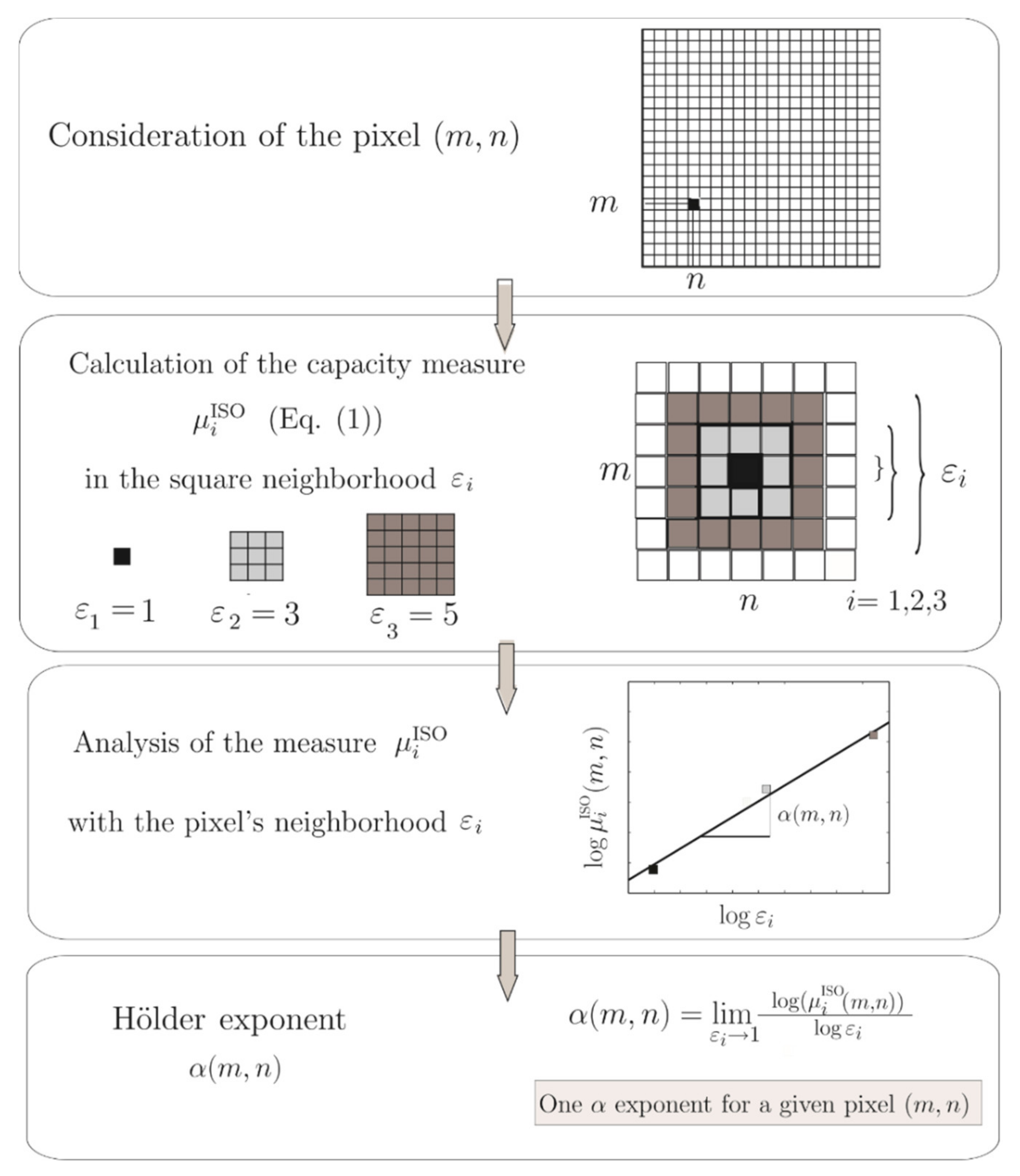
At the beginning of the multifractal image analysis, a measure is assigned to the image and, in the next steps, the measure regularity of this measure is analyzed as the information on the image’s complexity/inhomogeneity. It is worthwhile to underline the fact that various measures defined based on pixel intensities can be applied [38,40,46]. The local (pointwise) degree of regularity of a given measure is described by so-called Hölder exponent values, which strongly depend on the actual position on the image and allow researchers to identify points that differ from the background [40]. On the other hand, the distribution of Hölder exponents on the image is summarized in the form of the so-called multifractal spectrum, treated as the global characteristic of a measure’s regularity (image complexity/inhomogeneity) [38,40]. Global multifractal characteristics have already been applied to VHR optical data [47,48], mostly to distinguish between different land cover types. One can find also their application in the context of the study of forest cover, such as in Danila et al.’s work [49], or to perform the segmentation of plants’ disease images [50]. On the other hand, local multifractal description by using Hölder exponents has rarely been used, mainly to perform segmentation of medical data [38,40] or in the change detection aspects of satellite images [38,51]. 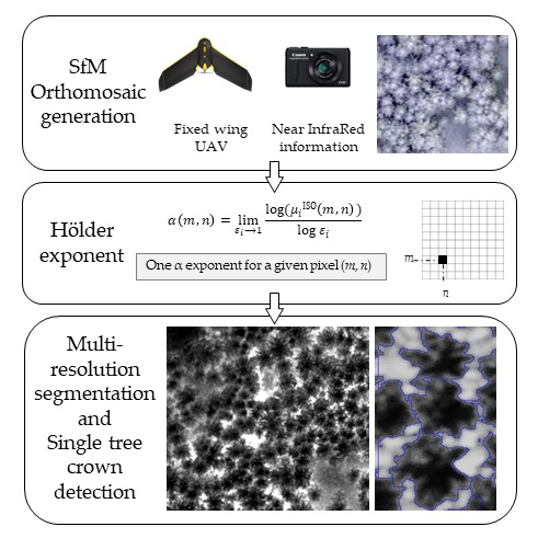Nevertheless, the results obtained in papers [38,40,51] suggest the usefulness of the Hölder exponent in the context of image content description. In particular, the authors of these studies underlined the fuller description of complex shapes, heterogeneous measures, and structures typical for satellite remote sensing. It is worth mentioning that, to the best of our knowledge, the Hölder exponent parameter has not been determined for VHR UAV-derived imagery yet or in the context of forest analysis. Therefore, in this study, we focus on the determination of the local Hölder exponent connected with multifractal theory and use it for the segmentation of single tree crowns from VHR UAV-derived imagery. More precisely, we propose to apply this quantitative descriptor as the unique input for the efficient identification of single tree crowns using only a cycle of multiresolution segmentation algorithms.

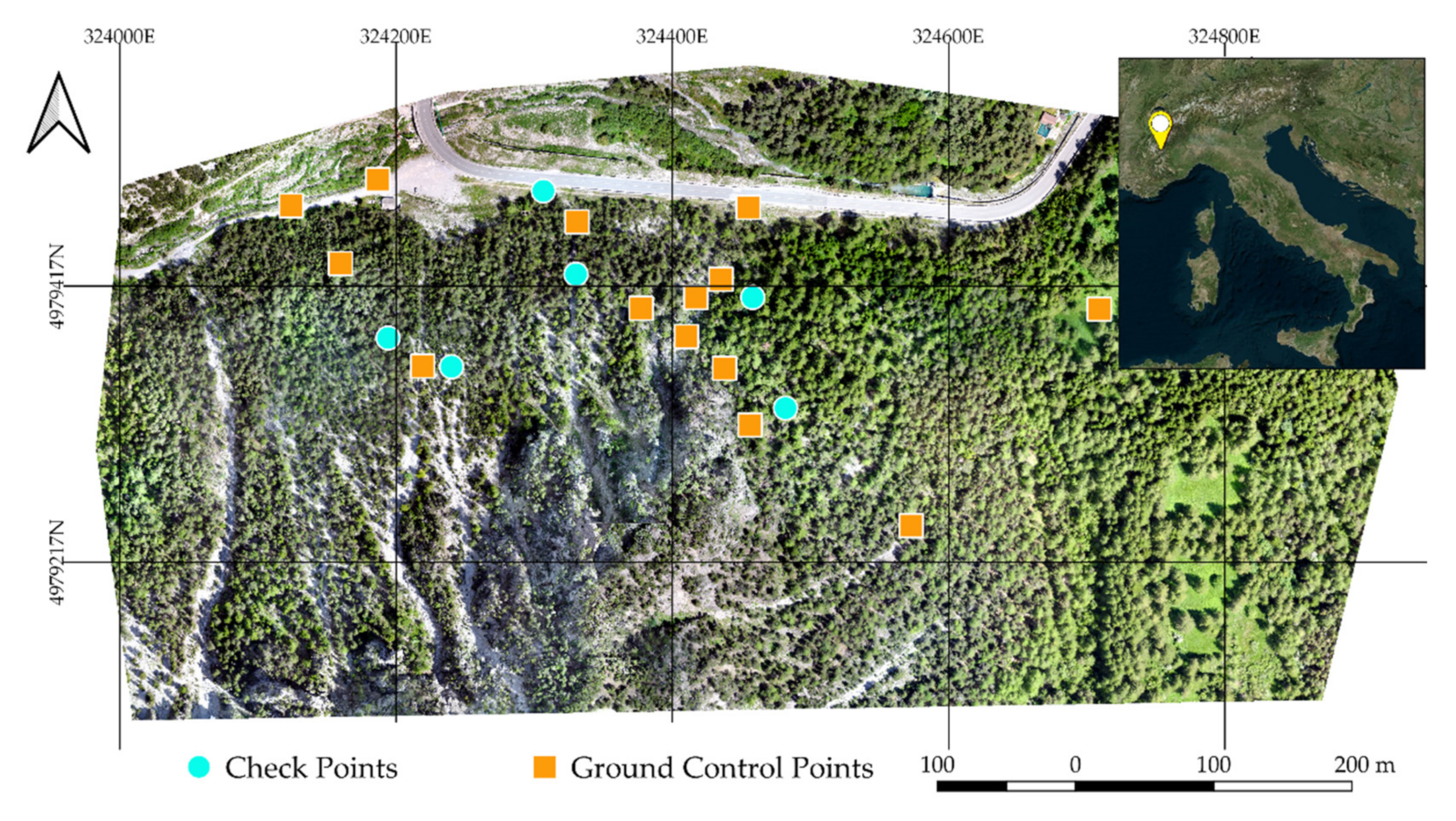
Study Site

This study was conducted in the North-Western Alps in a forest stand located in Cesana Torinese (TO) (44°56′46.1″ N 6°46′29.5″ E). The test study is a coniferous forest (Figure 1) dominated by silver fir (Abies alba Mill.), Norway spruce (Picea abies (L.) H. Karsten), and European larch (Larix decidua Mill.). Scots pines (Pinus sylvestris L.) and Swiss pines (Pinus cembra L.) are sporadically present. The study area extends to approximately 38 hectares. The forest stand is in a high-sloped mountainous area with north-facing exposure. The steep mountainsides make the area particularly prone to rockfall and avalanches.

2. Methods

2.1. UAV Flight and Photogrammetric Data Acquisition

UAV technology was used in this research in order to generate photogrammetric products to be used as input data for the segmentation of single tree crowns using multifractal analysis. The UAV system used was chosen to take into account the characteristics of the study area, regarding the topography, and the environmental conditions that could affect the execution of flights, the resolution of the products to be generated, and the sensors to be integrated. Besides the radiometric information regarding the visible part of the electromagnetic spectrum (red, green, blue), the near infrared (NIR) part was necessary. Indeed, NIR information can enhance the presence of vegetation in the image-processing phase, and, generally, NIR information helps distinguish shadows from dark objects, which have higher reflectance in the NIR. Due to the large area involved in this application and the steep terrain, with an elevation difference of about 400 m, we used a commercial fixed-wings solution, an eBee Plus made by senseFly. The eBee has a payload of up to 0.3 kg, a flight autonomy of 59 min, and it can reach a cruise speed of 40–110 km/h. Moreover, it does not require expert users, because take-off and landing are completely automatic, thanks to the built-in global navigation satellite system (GNSS) receiver.

Two different camera devices were employed for the collection of the RGB and NIR electromagnetic spectra. To perform the RGB flight, the eBee Plus was equipped with the RGB senseFly S.O.D.A. digital camera, with a sensor of 20 MP (5472 × 3648), a focal length of 10.6 mm, and a sensor size of 13.2 × 8.8 mm. A fixed number of frames per second equal to 0.25 fps was automatically acquired by the camera using a shutter cable. The flight with the eBee was planned using the eMotion software, considering a photogrammetric overlap between images of 80% in the lateral and longitudinal direction, an altitude of 220 m, a speed of 9 m/s, and an average ground resolution of 5 cm. Due to the extension of the area and the significant difference in height of the terrain, which could have adversely affected the autonomy of the battery by not allowing the flight to end, it was decided to survey the area through two distinct flights (

Table 2. Characteristics of the three flight plans (Avg. = average; Num. = number).

	S.O.D.A. _ 1st Flight	S.O.D.A. _ 2nd Flight	Canon S110 NIR
Avg. Height (m)	220	220	220
Avg. GSD (m)	5.47	5.47	6.29
Duration (min)	18	12	19
Area (ha)	60	40	76.4
Num. of images	221	137	176
Camera orientation	Nadir	Nadir	Nadir

). The flights were planned using as a base a digital surface model (DSM) of the area, from which the flight height was fixed. Given the steep terrain, the flight plan was created so that the survey lines of the flight path would be roughly parallel to the contour lines of similar elevation and then at constant height. In order to acquire NIR images, we used a commercial camera, the Canon S110 NIR. The main feature of the camera is that it has a modified filter that acquired the near infrared 850 nm, along with the red 625 nm and green 500 nm, light. The Canon S110 has a resolution of 12.1MP (4000 × 3000) and a focal length of 5.2 mm. Taking into account the characteristics of the camera sensor, the flight was performed with the eBee at a height of 220 m and a speed of 11 m/s, in order to guarantee an image overlap of 80% in both directions and an average ground sample distance (GSD) of about 6 cm. Table 2 shows the characteristics of the photogrammetric flights. The data acquisition is a key step of the photogrammetric process since the quality of the final result depends on it.

The data acquisition phase includes not only flights but, if necessary, the measurement of ground control points (GCPs) for the point cloud georeferencing and of check points (CPs) for the evaluation of the accuracy of the final results. To this purpose, before performing flights, 20 colored markers of 40 × 40 cm size were placed within the study area. A total of 14 of them were used as GCPs during the data processing phase, while 6 markers were employed as CPs for the validation of the model (Figure 1).

The position of the GCPs and CPs was acquired through a GNSS (global navigation satellite system) receiver using a real-time kinematic (RTK) (with a Global System for Mobile Communications GSM connection for real-time correction) approach, considering a session length of about 10 s for each point. The points’ coordinates were estimated with fixed-phase ambiguities. The centimeter-level accuracy ($\cong$3 cm) ensured a high level of precision for the georeferencing process.

2.2. Photogrammetric Data Processing

The aerial image acquisitions aimed to produce the RGB and RGN (red, green, NIR) orthomosaics. All the UAV data were post-processed through the structure from motion (SfM) approach [52]. These algorithms, which now are implemented in several commercial software, allow us to rapidly and accurately align the images, compute a three-dimensional dense point cloud and, then, to reconstruct a textured mesh of the object of study. In this case study, the photogrammetric process was carried out using the commercial solution AMP (Agisoft Metashape Professional).

The RGB datasets, acquired in two different flights, were processed together in the same project. A specific project was then dedicated to the processing of the RGN images. Nadiral images, in both projects, were aligned together, setting up the “high” level of accuracy of AMP, removing any limit on the key and tie points number. Subsequently, the measured GCPs and CPs were collimated in all the images, obtaining a 3D georeferenced model of known accuracy, as shown in

Table 3. Estimated residuals on the GCPs and CPs and characteristics of the obtained dense point clouds (where N. = number and RMSE = root mean square error).

Input Dataset	Data Resolution (Pixel)	N. of Images	RMSE on GCPs (m)			RMSE on CPs (m)			N. of Points (Dense Cloud)
			x	y	z	x	y	z
RGB	5472 × 3648	358	0.026	0.050	0.048	0.052	0.039	0.029	35,144,184
RGN	4048 × 3048	176	0.045	0.061	0.053	0.018	0.051	0.080	27,624,422

. The 3D dense point clouds was produced using a “high” level of detail to obtain products suitable for medium/large-scale representations (1:500) and an “aggressive” depth filtering in order to remove the noise due to the presence of dense vegetation. The next step involved the generation of a “high” quality mesh, from which we were able to generate the DSM of the study area. The results of the UAV image data processing were two orthomosaics in the RGB (Figure 1) and RGN (Figure 2) channels of the area of interest, in the WGS84—UTM 32N coordinates system. According to the accuracy of the model, the orthomosaics were produced with a resolution of 10 cm, setting the “mosaic” blending option in AMP. The borders of the orthomosaics were cut out from the study area to avoid distortion of the images and to obtain a regular shape.

Comparing the two orthomosaics obtained, it can be observed that the product in the RGN channels is incomplete with regard to the central part of the study area. In fact, it was not possible to align the RGN images related to this portion of the area, probably due to the considerable difference in altitude of the terrain, due to an almost vertical rock wall. However, the vegetation present in this area was rather low and sparse and, therefore, this does not affect the application of the algorithms described below. Finally, in addition to the two products already described, it was possible to generate the DTM of the area, using the dense point cloud as input data. Due to the complex terrain orography and the presence of dense vegetation, a semi-automatic approach was chosen. In the first step, the points belonging to the ground were classified with a specific algorithm in AMP by setting the maximum angle equal to 45 (i.e., the maximum angle between the terrain model and the line to connect a point with a point from a ground class). Subsequently, the classification was optimized manually in order to replace the points not correctly classified by the software. Exploiting the identified points of the ground, it was therefore possible to generate the DTM with a resolution of 10 cm.

2.3. Hölder Exponent Calculations

In this analysis, we focused on the local description of VHR UAV-derived imagery, using parameters related to multifractal formalism. More precisely, we determined the singularity strength α (known as the Hölder exponent), which depends on the pixel’s actual position in the structure (i.e., the single-band image), and this makes it possible to describe the local degree of regularity in the pixel’s neighborhood [40,51]. The procedure used to calculate the Hölder exponent α is graphically presented in Figure 3 and briefly summarized below. The Hölder exponent was calculated in Matlab©.

For each pixel $\left(m,n\right)$ of the NIR channel, we considered a square neighborhood of size ${\epsilon }_i=2i-1$, $i=1,2,\dots ,j$, where $j$ denotes the total number of squares, while ${\epsilon }_i$ is the size of a region centered on the pixel $\left(m,n\right)$. In this notation, ${\epsilon }_1=1$ denotes a square, which contains only a single pixel, ${\epsilon }_2=3$ represents a square of size $3\times 3$ containing the pixel’s neighbors, while ${\epsilon }_3=5$ is a square of size $5\times 5$, etc. It is worthwhile to stress that during the computation of $\alpha \left(m,n\right)$, various sizes of pixel neighborhoods $j$ as well as shapes can be applied, allowing us to describe localized or more widespread singularities. Here, we consider cases where the maximum neighborhood (maximum square size) of a pixel is $5\times 5$ ($j=3$). The next important aspect of Hölder exponent determination stated the use of various capacity measures (μ), which allows the emphasis of various effects on the image [40,48]. In the frame of this work, based on the initial tests, we applied the following type of capacity measure:

$${\mu }_i^{\mathrm{ISO}}\left(m,n\right)=\mathrm{card}\left\{\left(k,l\right)|g\left(m,n\right)\equiv g\left(k,l\right),\left(k,l\right)\in {\mathsf{\Omega }}_i\right\}$$

(1)

where $m,n$ denotes the pixel position, $g\left(k,l\right)$ is a gray-scale intensity at point $\left(k,l\right)$, and ${\mathsf{\Omega }}_i$ is the set of all pixels $\left(k,l\right)$ in the square. Capacity measure ISO (Equation (1)) gives the number of pixels in the considered neighborhood, which have the same values as the centered pixel $\left(m,n\right)$. ISO is the name of the capacity measure proposed by Véhel and Mignot (1994) [38] and Stojic et al., 2006 [40]. More precisely, the ISO measure, or ISO capacity measure, provides a presentation of a two-dimensional isosurface in the considered neighborhood window and is equal to the number of pixels with the same intensity as the analyzed pixel. A more detailed discussion about the used measures can be found in Véhel and Mignot (1994), Stojić et al. (2006), and Turner et al. (1998) [38,40,46].

After the calculation of the capacity measure ${\mu }_i^{\mathrm{ISO}}$, in the pixel neighborhood ${\epsilon }_i$, the discrete set of coarse Hölder exponents has been determined:

$${\alpha }_i\left(m,n\right)=\frac{\log \left({\mu }_i^{\mathrm{ISO}}\left(m,n\right)\right)}{\log {\epsilon }_i},$$

(2)

Finally, the limiting value of the Hölder exponent for each pixel from the NIR channel has been estimated using the formula:

$$\alpha \left(m,n\right)=\underset{{\epsilon }_i\to 1}{\lim }\frac{\log \left({\mu }_i^{\mathrm{ISO}}\left(m,n\right)\right)}{\log {\epsilon }_i},$$

(3)

as the slope of the linear regression through points on a log-log plot, where $\log {\epsilon }_i$ is plotted on the x-axis, and $\log {\mu }_i^{\mathrm{ISO}}\left(m,n\right)$ on the y-axis, as shown in the middle section of Figure 3 [51]. In the final step of analysis, a two-dimensional “α-image”, which collects Hölder exponents, has been calculated. To compute Hölder exponents, we used the software Matlab.

Additionally, as we underlined in the Introduction, next to the local Hölder exponent, the multifractal description enables us also to analyze the global distribution of the regularity in a whole scene and to summarize it in the form of the multifractal spectrum; see, e.g., Stojić et al. [40]. However, the usefulness of this function in the context of tree detection will be the topic of a separate analysis.

2.4. Segmentation Process

In the further steps of analysis, the Hölder exponent layer (α-image) determined by using the ISO capacity measure was used as the base feature for the ITD through the segmentation process. First, it was smoothed with a simple average filter to remove small variations on the crown surface. The degree of smoothness was defined by the size of the filter (3 × 3). The segmentation was realized with eCognition Developer software. Two segmentation steps accomplished the crown extraction. In the first step, the high-fractality pixels were separated from the low-fractality ones using the contrast split algorithm applied to the Hölder exponent layer, calculated on the infrared band. It was necessary to find the threshold value that represented the breakpoint between tree crowns and other elements.

Table 4. Algorithms and parameters used for the segmentation. The input band is the Hölder exponent image.

Algorithm	Parameters	Values	Notes
Contrast split segmentation	Minimum threshold	0.4
	Maximum threshold	1
	Step size	5
	Stepping type	Add
	Class for bright objects	Other
	Class for dark objects	Trees
Multiresolution segmentation	Scale parameter	11	Only trees class
	Shape	0.05
	Compactness	0.5
Chessboard segmentation	Object size	3	Only other class
Assign class	Use class	Temporary class	Only other class
	condition	Border to trees > 0 px
Grow region	Candidate classes	Temporary class	Only trees class
Remove object	Condition	Area < 80 px

shows the adopted parameters. The threshold parameters were selected to satisfy the spectral difference between crowns and other elements. The second step consisted of the extraction of the single crowns by applying the multiresolution segmentation algorithm (Table 4). Since the segmentation visually resulted in objects slightly smaller than the crowns’ RGB orthomosaics, they were up-sized to ensure the best match for the majority of the crowns. The objects were redefined by increasing the borders by 3 pixels and then removing those that measured less than 8 pixels. The growing phase interested only the tree pixels neighboring non-trees (class others) ones. The other pixels were segmented in objects of 3 × 3 pixel size, using chessboard segmentation algorithms. The crown objects were grown into the neighboring chessboard objects (Table 4). Finally, the segmentation was exported in the Quantum GIS (version 3.4.8) environment, where the jagged borders of the segments were smoothed (GDAL smoothing algorithm, set as three iterations with 0.5 offset) and validated.

2.5. Validation

Specific attention is given to the validation of the segmentation goodness methodology. Indeed, even if the literature is rich in methodologies for the evaluation of the goodness of segmentation and extraction of specific objects from imagery [53], a shared and accepted methodology for the accuracy assessment does not exist [54]. Besides this, the methods applied are quite similar to each other and, generally, they are based on the comparison between manually digitalized reference objects and the segmented objects [25,53,54,55,56,57]. We opted for a two-level validation, which takes into consideration qualitative and quantitative accuracy measures. The first level was based on the work of Ke at al. [25] and it consisted of a simple visual evaluation, while the second level assessment was a single tree quantitative method that compares several variables and it assessed the under-segmentation and over-segmentation. Both levels will be described in detail in the following sections. The accuracy assessments used as reference 200 crowns that were randomly selected but manually delineated (Figure 4).

To minimize the subjectivity, 200 random points were spread within the study area, and the crown on which the points fall was defined by manual segmentation, using as a background layer the RGN and RGB orthomosaics.

2.5.1. Visual Evaluation

The accuracy was evaluated in terms of correspondence between the reference crowns and the segmented ones. The evaluation methodology considers typical accuracy measures based on pixels (user’s and producer’s accuracy and F1 score) and applies them to measures based on objects. Particularly, the producer’s accuracy (PA) and the user’s accuracy (UA) are calculated using the following equations:

$$PA=\frac{M}{RC},$$

(4)

$$UA=\frac{M}{DC},$$

(5)

where PA is the producer’s accuracy, UA is the user’s accuracy, M is the number of matching crowns, RC is the number of reference crowns, and DC is the number of defined crowns. The relationship between UA and PA is described by the F1 score, from the following equation:

$$F1=\frac{2\times PA\times UA}{PA+UA}.$$

(6)

The situation shown in Figure 5a was considered as matching crowns (M), while the relationships of reference and segmented crowns in Figure 5b–d were considered as non-matching crowns. The segmented crowns were counted on the basis of their overlap with the reference crowns. For example, the segmented crowns in Figure 5b are zero, in Figure 5c are one, and in Figure 5d are three. Even if significant, these measures provide a partial view of the goodness of the segmentation. The omission and commission errors can describe more precisely the goodness of the segmentation. As illustrated by Ke and Quackenbush (2011) [25], we took into consideration four possible cases of the relationship between the reference dataset and the segmented one: (i) match, (ii) simple omission, (iii) omission through under-segmentation, and (iv) commission through over-segmentation (Figure 5).

2.5.2. Single Tree Quantitative Assessment Method

The accuracy evaluation approach is a two-dimensional spatial assessment on four metrics. It is based on the works of Persello et al. (2010), Clinton et al. (2010), and Yurtseven (2019) [53,54,55]. The areal difference, the perimeter, the distance of the centroid, the under-segmentation index, the over-segmentation index, and the completeness index are the evaluated metrics. The RMSE was calculated for the area and the perimeter.

The areal distance is the most common metric used as an indicator of segmentation goodness. It was calculated for the reference objects and segmented objects. In the case of over-segmentation, the reference area was compared to the sum of the segmented objects in correspondence with the reference tree.

The perimeter measures the length of the object borders; in the case of more than one crown corresponding to the reference, the segmented perimeter was calculated as the sum of the perimeters on every single object composing the crown in exam. With this approach, over-segmented objects have high RMSE values. It is worth mentioning that the perimeter metrics results should be considered with caution. Indeed, the values can vary according to the shape and the number of tree branches considered in the definition of the reference crowns.

The centroid distance represents the Euclidean distance between the gravitational centers of two shapes. The Euclidean distance between the centroids is calculated as the RMSE [55]; thus, it can be considered as the indicator of error on the distance between gravitational centers. In the event that more than one crown corresponded to the reference, the centroid distance was calculated between the reference crown and the closest centroid.

The RMSE of perimeter and area were calculated with the following formula:

$$RMSE \left(m\right)=\sqrt{\frac{{{\displaystyle \sum }}_{i=1}^n{(R_i-S_i)}^2}{n},}$$

(7)

where R_i is the value of metric m of the reference crown, and S_i is the metric m for the segmented crown. Four indicators for the evaluation of the goodness of the segmentation were applied. The over-segmentation index (OS), the under-segmentation index (US), the intersection over union index (J), and the completeness (D) were evaluated for each reference tree.

The OS and US were proposed by Clinton et al. (2010) and Persello (2010) [53,54]. Their estimations are based on the relationship between the area of the segmented (S) and reference objects (R). OS and US are described by the following equations:

$$OS=1-\frac{|R_i\cap S_i|}{\left|R_i\right|},$$

(8)

$$US=1-\frac{|R_i\cap S_i|}{\left|S_i\right|} ,$$

(9)

where $|R_i\cap S_i|$ is the overlapping area between the reference crown ($R_i$) and the segmented crown ($S_i$) of object i. Zero value describes a perfect match, while values that approach 1 indicate disagreements between the reference and the segmented object. The OS and US indices were considered the maximum, minimum, median, and average values.

The intersection over union (J), also known as the Jaccard index, quantifies also the false positives within the segmentation, and it is calculated as the ratio between the overlapping area ($R_i\cap S_i$) and the union area ($R_i\cup S_i$):

$$J=\frac{|R_i\cap S_i|}{|R_i\cup S_i|}$$

(10)

It is worthwhile to stress that when J is equal to 1, there is a perfect segmentation.

Finally, the completeness of the segmentation was evaluated through the completeness index (D) [53], calculated as the distance between the OS and the US, as follows:

$$D=\sqrt{\frac{O{S}_i{}^2+U{S}_i{}^2}{2}}.$$

(11)

The completeness index D should be interpreted as the closeness to an ideal segmentation result in relation to the reference set. When the D index is close to 0, it indicates a perfect segmentation.

2.5.3. Comparison with Segmentation Methodologies Based on Spectral, Textural and Elevation Information

To evaluate the goodness of the Hölder exponent segmentation, the results were checked against four different segmentations based on the elaboration of spectral, textural, and elevation information. Namely, the following were used as terms of comparison: (i) original spectral bands (red, green, NIR), (ii) normalized difference vegetation index; (iii) Haralick’s sum variance measure from GLCM [37], the CHM, and (iv) a multi-sourced approach that considers both the CHM and the sum variance. The goal of this validation was to evaluate on equal terms the performances for ITD of the Hölder exponent against other more common input data. Thus, the ITD from each of these measures was performed using the same ruleset applied for the Hölder exponent but with the tuning of the input parameters to achieve the best possible results. Basically, they were realized using contrast split and multi-resolution segmentation algorithms, with minor differences in the sequence to improve the final segmentation.

Table A1. Ruleset applied for the validation datasets.

Ruleset	Algorithm	Parameters	Values	Computing Time
RGN spectral information	Contrast split segmentation	Minimum threshold	40,000	7′54″
		Maximum threshold	100,000
		Step size	500
		Stepping type	Add
		Layer	NIR
		Class for bright objects	Trees
		Class for dark objects	Other
	Multiresolution segmentation	Scale parameter	1200	4′56″
		Layer	NIR, RED, GREEN
		Shape	0.05
		Compactness	0.5
	Remove object	Condition	Area < 80 px	1′43″
NDVI	Contrast split segmentation	Minimum threshold	0.18	11′29″
		Maximum threshold	0.25
		Step size	5
		Stepping type	Add
		Layer	NDVI
		Class for bright objects	Trees
		Class for dark objects	Other
	Remove object	Condition	Area < 80 px	6″
	Contrast split segmentation (Trees only)	Minimum threshold	0.26	7′89″
		Maximum threshold	1.00
		Step size	10
		Stepping type	Add
		Layer	NDVI
		Class for bright objects	Other
		Class for dark objects	Trees
	Remove object	Condition	Area < 80 px	6″
	Multiresolution segmentation (Trees only)	Scale parameter	11	4′28″
		Layer	NDVI
		Shape	0.05
		Compactness	0.5
	Remove object	Condition	Area < 80 px	6″
CHM	Contrast split segmentation	Minimum threshold	5	5′42″
		Maximum threshold	100
		Step size	5
		Stepping type	Add
		Layer	CHM
		Class for bright objects	Trees
		Class for dark objects	Other
	Multiresolution segmentation (Trees only)	Scale parameter	25	5′31″
		Layer	CHM
		Shape	0.05
		Compactness	0.5
	Remove object	Condition	Area < 80 px	<0.001″
Sum Variance GLCM	Contrast split segmentation	Minimum threshold	1	5′13″
		Maximum threshold	10
		Step size	5
		Stepping type	Add
		Layer	Sum variance
		Class for bright objects	Trees
		Class for dark objects	Other
	Multiresolution segmentation (Trees only)	Scale parameter	12	7′35″
		Layer	Sum variance
		Shape	0.05
		Compactness	0.5
	Remove object	Condition	Area < 80 px	<0.001″
Multi-sourced	Contrast split segmentation	Minimum threshold	5	1′29″
		Maximum threshold	100
		Step size	5
		Stepping type	Add
		Layer	CHM
		Class for bright objects	Trees
		Class for dark objects	Other
	Multiresolution segmentation	Scale parameter	12	5′29″
		Layer	Sum Variance with CHM local maxima as input thematic layer
		Shape	0.05
		Compactness	0.5
	Remove object	Condition	Area < 80 px	<0.001″

recaps the applied rules and parameters of each segmentation. As mentioned in the Introduction, the CHM was calculated as the difference between the digital surface model (DSM) and the digital terrain model (DTM). Then, the location of treetops was calculated by applying the local maxima algorithm and used in the multi-sourced segmentation. The NDVI, the sum variance GLCM measure, the CHM, and the local maxima were calculated using Quantum GIS. The selection of sum variance among all the GLCM existing measures is based on visual evaluation.

The comparison of the Hölder-based segmentation and the other segmentations (validation datasets) is based on the qualitative and quantitative measures for accuracy assessment described in Section 2.5, Section 2.5.1 and Section 2.5.2.

3. Results

3.1. Results of the Hölder Exponent Analysis and the Individual Tree Crown Definition

Figure 6c,f show the result in a sample area of Hölder exponents α. It is apparent that there is a contrast between the tree crowns and other elements of the background. The tops of the trees (black in c,f) have lower DN values compared to the lower branches (grey in c,f), which are generally lower than 0.2. The screes have DNs close to 0.3, while shaded areas vary from 0.4 to 1 (white areas in c,f). From the visual comparison of e,f, we can see that the Hölder exponent reduces the DN variability of tree crowns and enhances the contrast between crowns and shaded areas. This aspect facilitated the segmentation process. The entire segmentation process was realized in around 13 min.

Table 5. Computational time graphic restitution of each step (algorithm) of the segmentation process. Figures in blue have no classification. The class of trees is green, the class of other is yellow, the class of temporary is red.

Algorithm	Computing Time	Visual Restitution
Starting image	/
Contrast split segmentation	5′42″
Multiresolution segmentation	5′31″
Chessboard segmentation	12″
Assign class	5″
Grow region	6″
Remove object	<0.001″

shows the computational time for each of the applied algorithms and the graphic restitution of their results. The final segmented objects were 9215, with an average area of 21 m² and an average perimeter of 18 m. Figure 7 provides a sample of the segmentation results. From the very first visual evaluation, it appears that most of the crowns were detected. Some smaller crowns neighboring the scree appear slightly over-grown.

3.2. Results of Validation

The visual assessment of the segmentation provides positive results; indeed, only three crowns out of 200 references were not detected (simple omissions).

Table 6. Results from the visual evaluation of the Hölder exponent segmentation.

Validation of Individual Tree Crown Detection (ITD)	Hölder	Spectral	Normalized Difference Vegetation Index (NDVI)	Texture	Canopy Height Model (CHM)	Multi-Sourced
No. References	200	200	200	200	200	200
No. Segmented	228	289	529	248	247	330
Matches	157	85	39	64	57	68
Simple omission	3	1	9	3	38	8
Omission through under-segmentation	27	59	9	45	70	56
Commission through over-segmentation	13	55	143	88	35	68
Producer’s accuracy	0.785	0.425	0.195	0.320	0.285	0.340
User’s accuracy	0.689	0.294	0.074	0.258	0.231	0.206
F1 score	0.734	0.348	0.107	0.286	0.255	0.257

summarizes the results of the visual assessment of Hölder exponent segmentation (and of the validation datasets). Even if the simple omissions are rare, those produced through under-segmentation (OUS) are 27. The results underline the process’ tendency to under-segment. Although the PA is slightly better than the UA, it reaches 79%, against 69% of UA, while commission errors are much lower (only 13 out of 200). These affect the F1 score, which despite the OUS reach an acceptable value (73%).

The outcome is positively confirmed by the area-based analysis. As

Table 7. Root mean square error, the average and the % of error on the average, of the perimeter, the area, and the compactness metrics of the Hölder exponent segmentation and the validation datasets.

	Metric	RMSE	Average	RMSE/Average
Hölder	Area (m2)	2.903	21.099	14%
	Perimeter (m)	2.727	17.972	15%
Spectral	Area (m2)	4.367	21.299	21%
	Perimeter (m)	10.378	18.055	57%
NDVI	Area (m2)	3.758	21.407	18%
	Perimeter (m)	6.590	18.130	36%
Texture	Area (m2)	4.025	20.885	19%
	Perimeter (m)	5.574	17.863	31%
CHM	Area (m2)	2.090	23.126	9%
	Perimeter (m)	5.961	18.982	31%
Multi-Sourced	Area (m2)	3.432	21.772	16%
	Perimeter (m)	4.812	18.356	26%

shows, the RMSE on the area represents only 14% of the average dimension of the crowns: it is 3 m² over 21 m² of average crown extension. The RMSE on the perimeter is almost 3 m over the 18 m average perimeter, corresponding to 15%. This may be caused by the difficulties related to the definition of the reference tree, but also to the non-appropriate threshold value selected for the contrast split algorithm.

Table 8. Summary statistics of the over-segmentation index (OS), the under-segmentation index (US), the completeness index (D), the Jaccard index (J), and the distance between centroids.

Parameter	OS	US	D	J	Centroids Distance
average	0.084	0.284	0.227	0.661	0.830
min	0.000	0.002	0.037	0.047	0.021
max	0.533	0.953	0.674	0.935	4.077
median	0.056	0.214	0.181	0.718	0.458

presents the summary statistics regarding the over-segmentation (OS), under-segmentation (US), completeness (D), intersection over union (J) indices, and the distance between centroids. The minimum, maximum, and average values for each index were computed. What stands out is the high values of under-segmentation, which confirm the results of the visual estimation. The completeness (D) and the intersection over union (J) indices show significant positive results that confirm the accuracy of the ITD. The median values of D and J are respectively 0. 18 and 0.72. The mean distance between the centroids of the reference and segmented crowns is 83 cm, while the median distance is exceptionally 45 cm. This value is promising and indicates that the results are close to a 4-pixel error in crown localization.

Overall, the assessment depicts a positive scenario. The method used identifies the location of the crowns (centroid distance is below 50 cm) as well as their extensions, with a segmentation mean error of 14% on the area. Figure 8 presents the median values of the Jaccard index plotted against the area of the reference crowns. It can be seen that the proposed method is very efficient on larger crowns and prone to under-segmenting on smaller crowns. Indeed, the J index for the medium extension crowns (10–30 m²) is mostly above 0.5. The lowest values of J are recorded on very small crowns (less than 5m²).

Concerning the comparison with the ITD based on spectral, textural, and elevation information, Table 6 and Table 7 show respectively the results from the visual evaluation and the RMSE for the other validation segmentation methodologies. Generally, the Hölder exponent performs better as an input feature for the segmentation ruleset. Regarding the visual assessments, at equal condition, the results from the Hölder exponent outclassed those obtained from the other five validation datasets. For all methods, the producer’s accuracy shows higher values. Indeed, the number of objects describing the reference dataset, in any case, is less than 228 (the number of segments from Hölder analysis). The segmentation generated from the spectral information has the highest F1 score within the validation datasets, although it is very far from the F1 score of Hölder exponent segmentation (0.734 of Hölder against the 0.348 of spectral bands). The CHM methods show the larger value of simple omission, which might be attributable to the inaccuracies of photogrammetric DTM in areas with sloping.

The geometrical accuracy does not reflect the performance of the visual assessment. Indeed, the spectral information, even if quite-well performing in the F1 score, does not provide a good geometrical match with the reference crowns, while the geometrical accuracy of the CHM method outperforms the Hölder exponent results. It is worth underlining that the CHM samples amount to only 162 reference objects due to the simply omitted crowns. Within the RMSE analysis, the performance of the multi-sourced approach is the closest to that of the Hölder exponent.

Analyzing the median values of the indices in Figure 9, the under-segmentation (US) index does not reveal any significant difference between the Hölder exponent and other segmentation procedures. Meanwhile, in the analysis of the over-segmentation (OS), we have similar values from Hölder, sum variance, and the NDVI. The mixed and CHM approaches show the worst results in the completeness (D) and OS. The lowest value of centroid distance is that detected by CHM. It appears that the results of the segmentation based on the NDVI and the multi-sourced inputs (CHM and sum variance textural analysis) are the closest to those of the Hölder exponent. Nevertheless, no methods provided results as accurate as those of the Hölder exponent by using the same simple segmentation.

4. Discussion

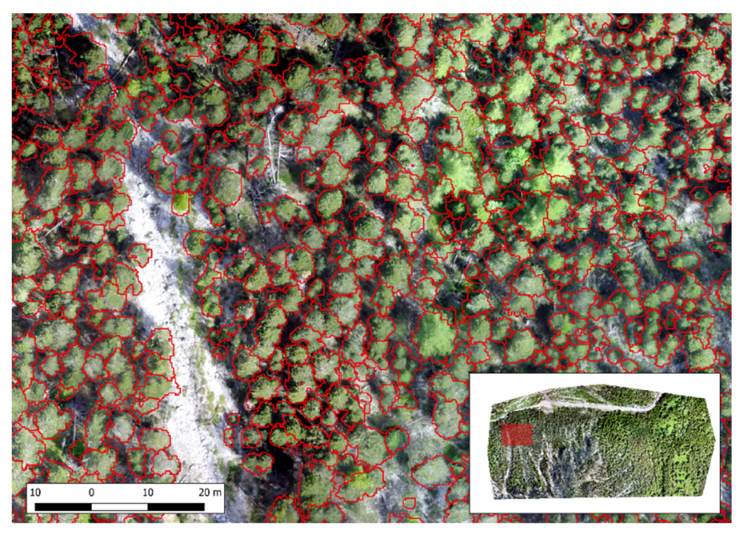
The results of this very first application of multifractals analysis of UAV imagery for the identification of single tree crowns are promising. In a relatively short time (around 13 min), it was possible to analyze 38 hectares of forest using one input layer only. The Hölder exponent analysis results in a clear image of the single tree crowns.

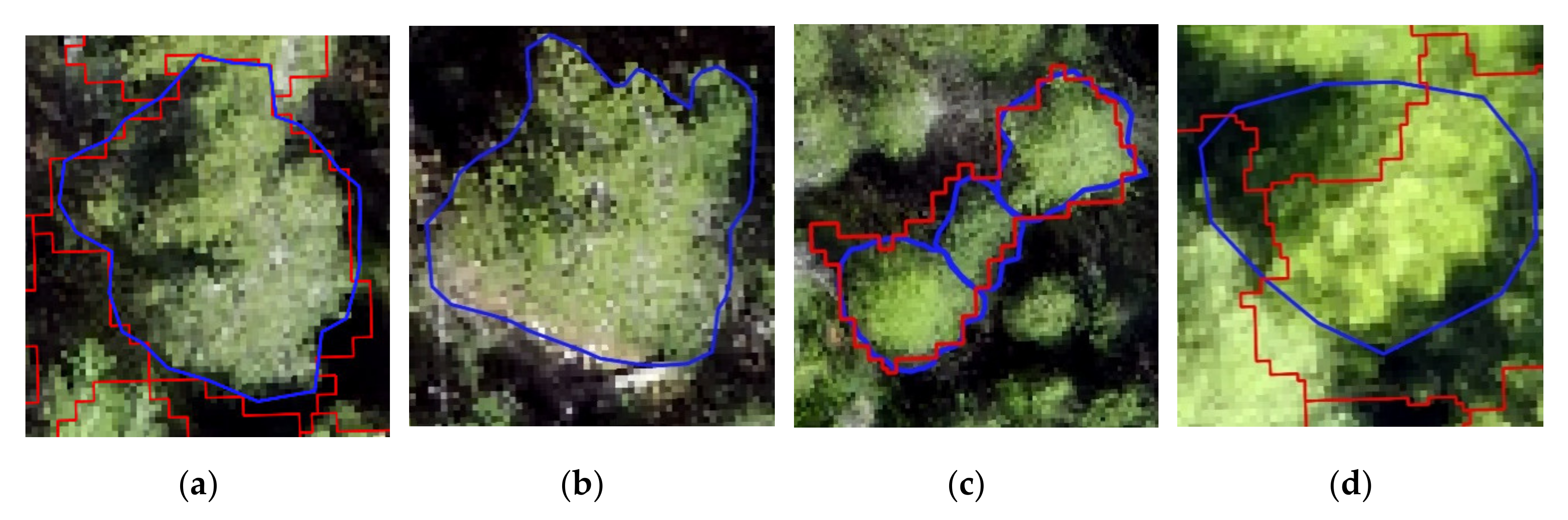
The pixels corresponding to the border of crowns present higher values of Hölder exponent. This most probably led to the underestimation of the dimension of the crowns after the contrast split segmentation. Nevertheless, growing the segmented objects of three pixels and smoothing them allowed us to limit such errors on most of the crowns.

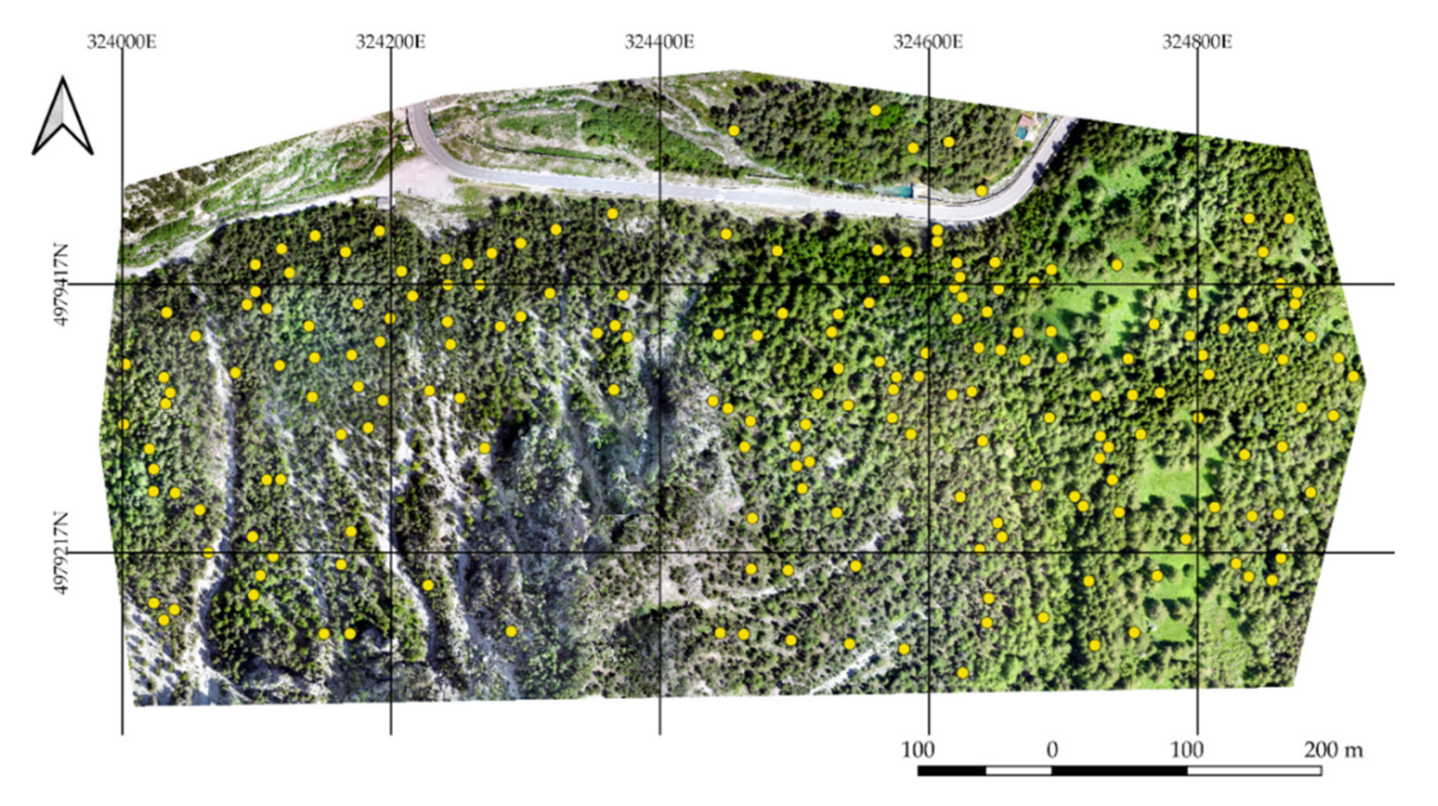
The assessment of the classification reveals promising results. The visual evaluation suggests more than 73% of the F1 score, which is in accordance with similar studies. Indeed, the very recent application of Qiu et al. [8] reaches an accuracy level of 76% in the VHR imagery segmentation, but this is also higher than the producer’s and user’s accuracy values obtained by Ke and Quackenbush in 2011 [25]. Mohan’s and Vieira’s works [5,56], respectively, reached 86% and 70% of the F1 score. It is worth mentioning that these comparisons should be interpreted with caution since many aspects can influence the goodness of the ITD. Firstly, the high level of subjectivity affects visual evaluations. Secondly, the characteristics of the study areas have a dominant role in the results of the ITD. Indeed, the illumination distortions due to the topography, the density, and the structure of the stand, along with the dominant species, can influence the results (and the goodness) of the segmentation. To fairly compare the results, we should have at least similar case studies; indeed, the works mentioned above are realized in flat or low-sloped areas over different types of forest stands. The selected ruleset is an additional influencing factor: it must be underlined that the segmentation applied in this study is intentionally plain and can be further improved, especially in the refining phase.

As already mentioned, the visual evaluation is limited in the assessment of the goodness of the segmentation. Several other aspects regarding the shape and the size of the individual tree crowns can be taken into account. The results of the quantitative assessment are clear: the positions of the crowns, as well as their extension, are very well-identified. As evidence, the median value of the centroid distance is 45 cm. Additionally, the area difference is not particularly relevant, since the RMSE represents only 14% of the average crown area. Thanks to the smoothing process, there is an evident match between the borders of the segmented and reference objects (the RMSE on the perimeter is almost 3 m). Although the validation indicates a good segmentation, it is important to underline the difficulty of the manual segmentation of references: even for the human eyes, the identification of single trees is not immediate. This is a quite common weakness of ITD (and, more generally, segmentation) researches. The RMSE of the perimeter has been calculated by Yurtseven et al. in their ITD research [55]. They obtain a 6-m RMSE on the perimeter metric, even though they had the chance to identify the crowns on a 1.2 cm/pixel RGB orthomosaic, as an additional demonstration of the subjectivity and complexity of the reference dataset identification. Compared to the existing works of ITD and segmentation, the Hölder exponent provides results that are perfectly in line with the literature.

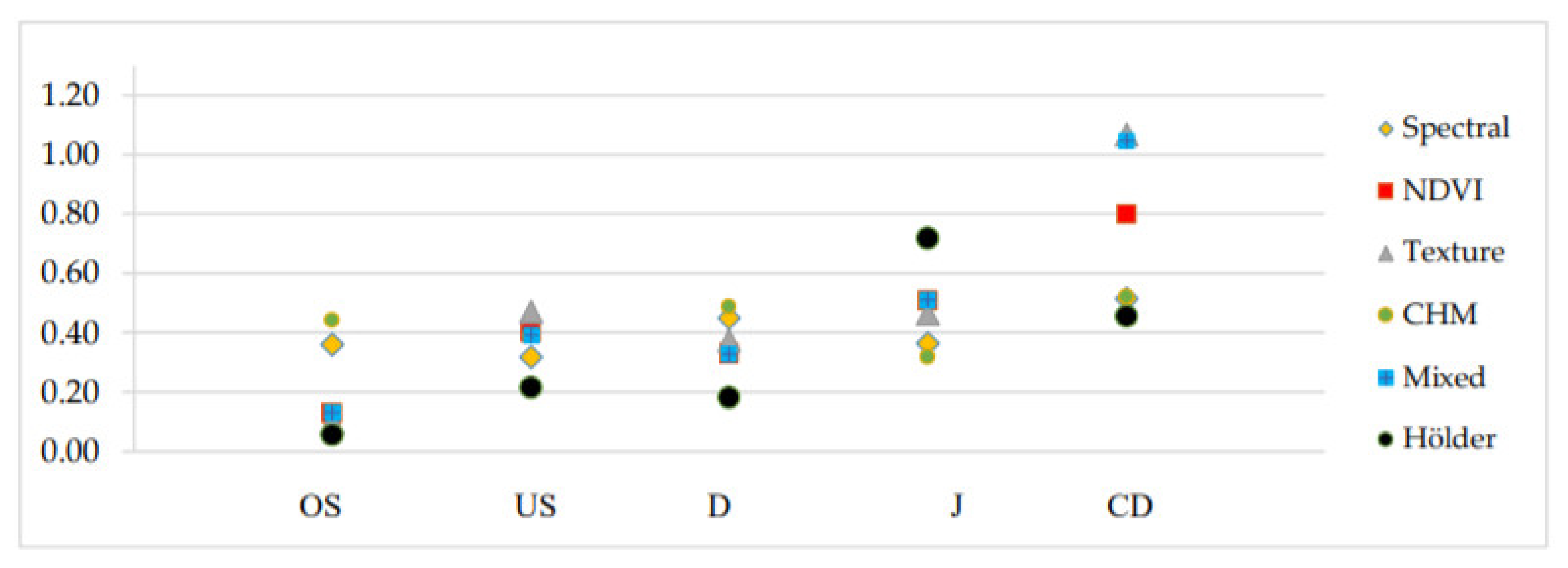
The tendency of the proposed method to under-segment more than over-segment is evident also from the comparison of US (0.284) and OS indices (0.084). The Jaccard indicator is 72%, a result which is in line with other studies, despite of the high variability of the delineation of the reference dataset. Hussin et al. [57] applied the OS and US indicators to the assessment of tree segmentation, using satellite imagery of 2-m resolution, and they obtained comparable values for both under-segmentation and over-segmentation. However, in their work, they faced the opposite situation: over-segmentation errors are more dominant than under-segmentation ones. Persello et al. and Clinton et al. [53,54] obtained very similar OS and US results too, even though both studies focused on the segmentation (and classification) of satellite imagery in urban areas. The 0.18 median value resulting from the D index mirrors the values in the literature and it is a relatively good result. The literature reports values between 0.31 and 0.42. Again, these metrics and comparison should be interpreted with caution since they are the results of segmentation from satellite imagery and this does not include the extraction of single tree crowns. Finally, the Jaccard index, or intersection over union index, values vary between 0.05 and 0.95, with 0.72 as the median value.

On the same segmentation process, the results of Hölder exponent segmentation clearly outclass the others from spectral, textural, and CHM information. From this first application, it emerged that Hölder exponent can facilitate the ITD from UAV VHR imagery. Indeed, by applying a basic segmentation process, we obtained satisfying results in line with the literature, but in a relatively short time and with one elevation-independent input layer only. With this approach, the ITD from optical imagery of densely forested areas might be more accurate than simple spectral and elevation-based analysis. Naturally, this work should not be interpreted as an attempt to discredit ITD from the spectral and CHM dataset but as an alternative and computational low-demanding solution to ITD.

5. Conclusions

The purpose of the current study was to determine the local Hölder exponent connected with multifractal theory and use it for the description of VHR UAV optical imagery and the detection of individual single tree crowns. Although multifractals analysis has been applied in image processing in many different fields, from the medical field to satellite remote sensing, their use for UAV imagery has not been confirmed. The high radiometric variability is typical of the VHR datasets that often introduced noise, which is reflected in imprecision in automatic segmentation and classifications. This aspect was reduced by the multifractal analysis, and the single tree crowns clearly emerged. The Hölder exponent makes the segmentation easier and simpler based on the threshold of the local contrast. The results of the validation are generally satisfying and in line with similar research realized on optical and LiDAR datasets. The main detected errors were classified as under-segmentation problems.

Unfortunately, as far as we know, little research on ITD applies quantitative methods similar to those that we used for the assessment of the segmentation. Indeed, a strong limit in the assessment of ITD is the subjectivity in the definition of the reference dataset. Nevertheless, the obtained results confirm the Hölder exponent applied to VHR imagery as a potentially powerful tool in the ITD. The analysis required a relatively short time and low computational power. Additionally, RGB and NIR sensors mounted on UAVs are systems that are becoming cheaper and easily operable. The present study lays the groundwork for future research into ITD from VHR optical imagery. Since this is its very first application, several aspects still need to be addressed and further investigated. Our focus area was coniferous-dominant, with crowns that present fractal patterns from a nadiral view; we might have very different results on broadleaves forests. Moreover, we worked with the Hölder exponent only and it would be interesting to explore additional measures in different forest types and try to work with different spatial resolutions, spectral bands, and parameters. Additionally, it may be worth testing different neighborhood sizes for the calculation of the Hölder exponent to verify its influence on the analysis. It is worth mentioning that multifractal descriptors can be applied in parallel with the DEM-based method, through the definition of the treetops from the CHM and the delineation of the crown boundaries with segmentation from the multifractal analysis. This may help to ease up the process with the optical sensor on the individual tree crown detection. Among others, some of the most interesting applications of the Hölder–ITD might be for the update of forestry inventories at the local scale and the multi-temporal monitoring of specific forest indicators (and parameters) related to crown size. An additional application of this methodology might be VHR satellite imagery. Several additional analyses and tests can still be conducted, and it is our intention to do so—our research is only the first application that moves in this direction.

References

1. D’Oleire-Oltmanns, S.; Marzolff, I.; Peter, K.D.; Ries, J.B. Unmanned Aerial Vehicle (UAV) for Monitoring Soil Erosion in Morocco. Remote Sens. 2012, 4, 3390–3416. [Google Scholar] [CrossRef] [Green Version]
2. Hruska, R.; Mitchell, J.; Anderson, M.; Glenn, N.F. Radiometric and Geometric Analysis of Hyperspectral Imagery Acquired from an Unmanned Aerial Vehicle. Remote Sens. 2012, 4, 2736–2752. [Google Scholar] [CrossRef] [Green Version]
3. Skoglar, P.; Orguner, U.; Törnqvist, D.; Gustafsson, F. Road Target Search and Tracking with Gimballed Vision Sensor on an Unmanned Aerial Vehicle. Remote Sens. 2012, 4, 2076–2111. [Google Scholar] [CrossRef] [Green Version]
4. De Luca, G.; Silva, J.M.N.; Cerasoli, S.; Araújo, J.; Campos, J.; Di Fazio, S.; Modica, G. Object-Based Land Cover Classification of Cork Oak Woodlands using UAV Imagery and Orfeo ToolBox. Remote Sens. 2019, 11, 1238. [Google Scholar] [CrossRef] [Green Version]
5. Mohan, M.; Silva, C.A.; Klauberg, C.; Jat, P.; Catts, G.; Cardil, A.; Hudak, A.T.; Dia, M. Individual Tree Detection from Unmanned Aerial Vehicle (UAV) Derived Canopy Height Model in an Open Canopy Mixed Conifer Forest. Forests 2017, 8, 340. [Google Scholar] [CrossRef] [Green Version]
6. Magnard, C.; Morsdorf, F.; Small, D.; Stilla, U.; Schaepman, M.E.; Meier, E. Single tree identification using airborne multibaseline SAR interferometry data. Remote Sens. Environ. 2016, 186, 567–580. [Google Scholar] [CrossRef]
7. Sačkov, I.; Bucha, T.; Király, G.; Brolly, G.; Raši, R. Individual tree and crown identification in the Danube floodplain forests based on airborne laser scanning data. In Proceedings of the Conference: EARSeL 34th Symposium, Warsaw, Poland, 16–20 June 2014. [Google Scholar]
8. Qiu, L.; Jing, L.; Hu, B.; Li, H.; Tang, Y. A New Individual Tree Crown Delineation Method for High Resolution Multispectral Imagery. Remote Sens. 2020, 12, 585. [Google Scholar] [CrossRef] [Green Version]
9. Panagiotidis, D.; Abdollahnejad, A.; Surový, P.; Chiteculo, V. Determining tree height and crown diameter from high-resolution UAV imagery. Int. J. Remote Sens. 2017, 38, 2392–2410. [Google Scholar] [CrossRef]
10. Bottai, L.; Arcidiaco, L.; Chiesi, M.; Maselli, F. Application of a single-tree identification algorithm to LiDAR data for the simulation of stem volume current annual increment. J. Appl. Remote Sens. 2013, 7, 073699. [Google Scholar] [CrossRef]
11. Moe, K.T.; Owari, T.; Furuya, N.; Hiroshima, T. Comparing Individual Tree Height Information Derived from Field Surveys, LiDAR and UAV-DAP for High-Value Timber Species in Northern Japan. Forests 2020, 11, 223. [Google Scholar] [CrossRef] [Green Version]
12. Yao, W.; Krzystek, P.; Heurich, M. Tree species classification and estimation of stem volume and DBH based on single tree extraction by exploiting airborne full-waveform LiDAR data. Remote Sens. Environ. 2012, 123, 368–380. [Google Scholar] [CrossRef]
13. Dong, T.; Zhang, X.; Ding, Z.; Fan, J. Multi-layered tree crown extraction from LiDAR data using graph-based segmentation. Comput. Electron. Agric. 2020, 170, 105213. [Google Scholar] [CrossRef]
14. Zaforemska, A.; Xiao, W.; Gaulton, R. Individual Tree Detection from UAV Lidar Data in a Mixed Species Woodland. ISPRS Int. Arch. Photogramm. Remote Sens. Spat. Inf. Sci. 2019, XLII-2/W13, 657–663. [Google Scholar] [CrossRef] [Green Version]
15. Wang, X.-H.; Zhang, Y.-Z.; Xu, M.-M. A Multi-Threshold Segmentation for Tree-Level Parameter Extraction in a Deciduous Forest Using Small-Footprint Airborne LiDAR Data. Remote Sens. 2019, 11, 2109. [Google Scholar] [CrossRef] [Green Version]
16. Abdullah, S.S.; Tahar, K.N.; Rashid, M.F.A.; Osoman, M.A. Capabilities of UAV-Based Watershed Segmentation Method for Estimating Tree Crown: A Case Study of Oil Palm Tree. IOP Conf. Ser. Earth Environ. Sci. 2019, 385, 012015. [Google Scholar] [CrossRef]
17. Grznárová, A.; Mokroš, M.; Surový, P.; Slavík, M.; Pondelík, M.; Merganič, J. The Crown Diameter Estimation from Fixed Wing Type of UAV Imagery. ISPRS Int. Arch. Photogramm. Remote Sens. Spat. Inf. Sci. 2019, XLII-2/W13, 337–341. [Google Scholar] [CrossRef] [Green Version]
18. Fonstad, M.A.; Dietrich, J.T.; Courville, B.C.; Jensen, J.L.; Carbonneau, P.E. Topographic structure from motion: A new development in photogrammetric measurement. Earth Surf. Process. Landf. 2013, 38, 421–430. [Google Scholar] [CrossRef] [Green Version]
19. Iglhaut, J.; Cabo, C.; Puliti, S.; Piermattei, L.; O’Connor, J.; Rosette, J. Structure from Motion Photogrammetry in Forestry: A Review. Curr. For. Rep. 2019, 5, 155–168. [Google Scholar] [CrossRef] [Green Version]
20. Snavely, K.N. Scene Reconstruction and Visualization from Internet Photo Collections. Ph.D. Thesis, University of Washington, Seattle, WA, USA, 2008. [Google Scholar]
21. Agarwal, S.; Snavely, N.; Seitz, S.M.; Szeliski, R. Bundle adjustment in the large. In Proceedings of the 11th European conference on Computer Vision: Part II, Heraklion, Crete, Greece, 5–11 September 2010; pp. 29–42. [Google Scholar]
22. Wu, C.; Agarwal, S.; Curless, B.; Seitz, S.M. Multicore bundle adjustment. In Proceedings of the CVPR 2011, Colorado Springs, CO, USA, 20–25 June 2011; pp. 3057–3064. [Google Scholar]
23. Seitz, S.M.; Curless, B.; Diebel, J.; Scharstein, D.; Szeliski, R. A Comparison and Evaluation of Multi-View Stereo Reconstruction Algorithms. In Proceedings of the 2006 IEEE Computer Society Conference on Computer Vision and Pattern Recognition—Volume 1 (CVPR’06); IEEE: New York, NY, USA, 2006; Volume 1, pp. 519–528. [Google Scholar]
24. Vastaranta, M.; Kankare, V.; Holopainen, M.; Yu, X.; Hyyppä, J.; Hyyppä, H. Combination of individual tree detection and area-based approach in imputation of forest variables using airborne laser data. ISPRS J. Photogramm. Remote Sens. 2012, 67, 73–79. [Google Scholar] [CrossRef]
25. Ke, Y.; Quackenbush, L.J. A comparison of three methods for automatic tree crown detection and delineation from high spatial resolution imagery. Int. J. Remote Sens. 2011, 32, 3625–3647. [Google Scholar] [CrossRef]
26. Torres-Sánchez, J.; López-Granados, F.; Peña, J.M. An automatic object-based method for optimal thresholding in UAV images: Application for vegetation detection in herbaceous crops. Comput. Electron. Agric. 2015, 114, 43–52. [Google Scholar] [CrossRef]
27. Pouliot, D.A.; King, D.J.; Bell, F.W.; Pitt, D.G. Automated tree crown detection and delineation in high-resolution digital camera imagery of coniferous forest regeneration. Remote Sens. Environ. 2002, 82, 322–334. [Google Scholar] [CrossRef]
28. Wolf (né Straub), B.-M.; Heipke, C. Automatic extraction and delineation of single trees from remote sensing data. Mach. Vis. Appl. 2007, 18, 317–330. [Google Scholar] [CrossRef]
29. White, J.C.; Wulder, M.A.; Vastaranta, M.; Coops, N.C.; Pitt, D.; Woods, M. The Utility of Image-Based Point Clouds for Forest Inventory: A Comparison with Airborne Laser Scanning. Forests 2013, 4, 518–536. [Google Scholar] [CrossRef] [Green Version]
30. Pearse, G.D.; Dash, J.P.; Persson, H.J.; Watt, M.S. Comparison of high-density LiDAR and satellite photogrammetry for forest inventory. ISPRS J. Photogramm. Remote Sens. 2018, 142, 257–267. [Google Scholar] [CrossRef]
31. Campbell, J.B.; Wynne, R.H. Introduction to Remote Sensing, 5th ed.; Guilford Press: New York, NY, USA, 2011; ISBN 978-1-60918-176-5. [Google Scholar]
32. Maschler, J.; Atzberger, C.; Immitzer, M. Individual Tree Crown Segmentation and Classification of 13 Tree Species Using Airborne Hyperspectral Data. Remote Sens. 2018, 10, 1218. [Google Scholar] [CrossRef] [Green Version]
33. Dorren, L.K.A.; Maier, B.; Seijmonsbergen, A.C. Improved Landsat-based forest mapping in steep mountainous terrain using object-based classification. For. Ecol. Manag. 2003, 183, 31–46. [Google Scholar] [CrossRef]
34. Itten, K.I.; Meyer, P. Geometric and radiometric correction of TM data of mountainous forested areas. IEEE Trans. Geosci. Remote Sens. 1993, 31, 764–770. [Google Scholar] [CrossRef]
35. Lewiński, S.; Aleksandrowicz, S.; Banaszkiewicz, M. Testing Texture of VHR Panchromatic Data as a Feature of Land Cover Classification. Acta Geophys. 2015, 63, 547–567. [Google Scholar] [CrossRef] [Green Version]
36. Blaschke, T. Object based image analysis for remote sensing. ISPRS J. Photogramm. Remote Sens. 2010, 65, 2–16. [Google Scholar] [CrossRef] [Green Version]
37. Haralick, R.M.; Shanmugam, K.; Dinstein, I. Textural Features for Image Classification. IEEE Trans. Syst. Man Cybern. 1973, SMC-3, 610–621. [Google Scholar] [CrossRef] [Green Version]
38. Véhel, J.L.; Mignot, P. Multifractal Segmentation of Images. Fractals 1994, 2, 371–377. [Google Scholar] [CrossRef]
39. Voorons, M.; Germain, M.; Benie, G.B.; Fung, K. Segmentation of high resolution images based on the multifractal analysis. In Proceedings of the IGARSS 2003. 2003 IEEE International Geoscience and Remote Sensing Symposium; IEEE: Piscataway, NJ, USA, 2013; Volume 6, pp. 3531–3533. [Google Scholar]
40. Stojić, T.; Reljin, I.; Reljin, B. Adaptation of multifractal analysis to segmentation of microcalcifications in digital mammograms. Phys. Stat. Mech. Appl. 2006, 367, 494–508. [Google Scholar] [CrossRef]
41. Mandelbrot, B.B. The Fractal Geometry of Nature; W.H. Freeman: San Francisco, CA, USA, 1982. [Google Scholar]
42. Sun, W.; Xu, G.; Gong, P.; Liang, S. Fractal analysis of remotely sensed images: A review of methods and applications. Int. J. Remote Sens. 2006, 27, 4963–4990. [Google Scholar] [CrossRef]
43. Keller, J.M.; Chen, S.; Crownover, R.M. Texture description and segmentation through fractal geometry. Comput. Vis. Graph. Image Process. 1989, 45, 150–166. [Google Scholar] [CrossRef]
44. Lorimer, N.D.; Haight, R.G.; Leary, R.A. The Fractal Forest: Fractal Geometry and Applications in Forest Science; General Technical Report NC-170; USDA Forest Service: St. Paul, MN, USA, 1994.
45. Zeide, B.; Pfeifer, P. A Method for Estimation of Fractal Dimension of Tree Crowns. For. Sci. 1991, 37, 1253–1265. [Google Scholar] [CrossRef]
46. Turner, M.J.; Blackledge, J.M.; Andrews, P.R. Fractal Geometry in Digital Imaging; Academic Press: San Diego, CA, USA, 1998; ISBN 978-0-12-703970-1. [Google Scholar]
47. Wawrzaszek, A.; Aleksandrowicz, S.; Krupiński, M.; Drzewiecki, W. Influence of Image Filtering on Land Cover Classification when Using Fractal and Multifractal Features. Photogramm. Fernerkund. Geoinf. 2014, 2014, 101–115. [Google Scholar] [CrossRef]
48. Jenerowicz, M.; Wawrzaszek, A.; Krupiński, M.; Aleksandrowicz, S.; Drzewiecki, W. Comparison of mathematical morphology with the local multifractal description applied to the image samples processing. In Proceedings of the Photonics Applications in Astronomy, Communications, Industry, and High-Energy Physics Experiments 2019; Romaniuk, R.S., Linczuk, M., Eds.; SPIE: Wilga, Poland, 2019; p. 29. [Google Scholar]
49. Danila, E.; Hahuie, V.; Georgescu, P.L.; Moraru, L. Survey of Forest Cover Changes by Means of Multifractal Analysis. Carpathian J. Earth Environ. Sci. 2019, 14, 51–60. [Google Scholar] [CrossRef]
50. Wang, F.; Li, J.-W.; Shi, W.; Liao, G.-P. Leaf image segmentation method based on multifractal detrended fluctuation analysis. J. Appl. Phys. 2013, 114, 214905. [Google Scholar] [CrossRef]
51. Aleksandrowicz, S.; Wawrzaszek, A.; Drzewiecki, W.; Krupinski, M. Change Detection Using Global and Local Multifractal Description. IEEE Geosci. Remote Sens. Lett. 2016, 13, 1183–1187. [Google Scholar] [CrossRef]
52. Turner, D.; Lucieer, A.; Watson, C. An Automated Technique for Generating Georectified Mosaics from Ultra-High Resolution Unmanned Aerial Vehicle (UAV) Imagery, Based on Structure from Motion (SfM) Point Clouds. Remote Sens. 2012, 4, 1392–1410. [Google Scholar] [CrossRef] [Green Version]
53. Clinton, N.; Holt, A.; Scarborough, J.; Yan, L.; Gong, P. Accuracy Assessment Measures for Object-based Image Segmentation Goodness. Available online: https://www.ingentaconnect.com/content/asprs/pers/2010/00000076/00000003/art00004# (accessed on 24 March 2020).
54. Persello, C.; Bruzzone, L. A Novel Protocol for Accuracy Assessment in Classification of Very High Resolution Images. IEEE Trans. Geosci. Remote Sens. 2010, 48, 1232–1244. [Google Scholar] [CrossRef]
55. Yurtseven, H.; Akgul, M.; Coban, S.; Gulci, S. Determination and accuracy analysis of individual tree crown parameters using UAV based imagery and OBIA techniques. Measurement 2019, 145, 651–664. [Google Scholar] [CrossRef]
56. Da Vieira, G.S.; Rocha, B.M.; Soares, F.; Lima, J.C.; Pedrini, H.; Costa, R.; Ferreira, J. Extending the Aerial Image Analysis from the Detection of Tree Crowns. In Proceedings of the 2019 IEEE 31st International Conference on Tools with Artificial Intelligence (ICTAI), Portland, OR, USA, 4–6 November 2019; pp. 1681–1685. [Google Scholar]
57. Hussin, Y.A.; Gilani, H.; van Leeuwen, L.; Murthy, M.S.R.; Shah, R.; Baral, S.; Tsendbazar, N.-E.; Shrestha, S.; Shah, S.K.; Qamer, F.M. Evaluation of object-based image analysis techniques on very high-resolution satellite image for biomass estimation in a watershed of hilly forest of Nepal. Appl. Geomat. 2014, 6, 59–68. [Google Scholar] [CrossRef]
Figure 1. The study area in Cesana Torinese. The light blue circles are the check points (CPs) and the orange squares are the ground control points (GCPs).
Remotesensing 12 02407 g001
Figure 2. Resulting RGN orthomosaic.
Remotesensing 12 02407 g002
Figure 3. The procedure used to calculate the Hölder exponent α , adapted from Figure 1b in Aleksandrowicz et al. [51]. Here, m and n denote the pixel position on the image; μ i ISO is the capacity measure calculated by using Equation (1) in the pixel neighborhood of ε i size, where i = 1 , 2 , 3 .
Remotesensing 12 02407 g003
Figure 4. Yellow points indicate the location of the reference crowns within the study area.
Remotesensing 12 02407 g004
Figure 5. Possible cases of the relationship between reference crowns (blue border) and segmented crowns (red border). (a) Match. (b) Simple omission. (c) Omission through under-segmentation. (d) Commission through over-segmentation.
Remotesensing 12 02407 g005
Figure 6. (a,d) Details of RGB dataset; (b,e) Details of RGN dataset of the same area presented in (a,d); (c,f) Map of the Hölder exponents determined for the area presented in (a,d). The Hölder exponent layer restitution is in greyscale visualization, where 0 is black and 1 is white. The shadows are mitigated and the single crowns are easily identified, as well as the grasslands that are large areas of low DNs.
Remotesensing 12 02407 g006
Figure 7. Detail of the delineation of single crowns (red border) on RGB orthomosaic. The red square in the bottom-right corner indicates the location of the sample area within the entire study area.
Remotesensing 12 02407 g007
Figure 8. Distribution of the Jaccard index (y-axis) values according to the crown size (x-axis).
Remotesensing 12 02407 g008
Figure 9. The plot of the over-segmentation index (OS), under-segmentation index (US), ompleteness index (D), Jaccard index (J), and the distance between centroids (CD) calculated on the Hölder exponent dataset and the validation datasets (spectral information, NDVI, sum variance textural information, CHM, and the mixed input data).
Remotesensing 12 02407 g009