Individual Tree-Crown Detection and Species Classification in Very High-Resolution Remote Sensing Imagery Using a Deep Learning Ensemble Model

Abstract

Traditional methods for individual tree-crown (ITC) detection (image classification, segmentation, template matching, etc.) applied to very high-resolution remote sensing imagery have been shown to struggle in disparate landscape types or image resolutions due to scale problems and information complexity. Deep learning promised to overcome these shortcomings due to its superior performance and versatility, proven with reported detection rates of ~90%. However, such models still find their limits in transferability across study areas, because of different tree conditions (e.g., isolated trees vs. compact forests) and/or resolutions of the input data. This study introduces a highly replicable deep learning ensemble design for ITC detection and species classification based on the established single shot detector (SSD) model. The ensemble model design is based on varying the input data for the SSD models, coupled with a voting strategy for the output predictions. Very high-resolution unmanned aerial vehicles (UAV), aerial remote sensing imagery and elevation data are used in different combinations to test the performance of the ensemble models in three study sites with highly contrasting spatial patterns. The results show that ensemble models perform better than any single SSD model, regardless of the local tree conditions or image resolution. The detection performance and the accuracy rates improved by 3–18% with only as few as two participant single models, regardless of the study site. However, when more than two models were included, the performance of the ensemble models only improved slightly and even dropped.

1. Introduction

The identification of individual tree-crowns (ITC) is an important research topic in forestry, remote sensing and computer vision [1]. It is a requirement in forest management and monitoring as it provides key forest inventory information [2]. Accurate ITC information can also sustain basic research, such as the metabolic theory of ecology [3].

The increasing availability of very high-resolution remote sensing data has stimulated the development of automated techniques for ITC identification [4]. Light Detection and Ranging (LiDAR) data, either in the form of rasterized 2D models or as a point cloud, enables the accurate identification of trees, as well as quantifying other structural parameters [5]. Thus, LiDAR technology, and mainly its aerial version (aerial laser scanning—ALS) has been the main source of data for ITC studies [1]. A more affordable alternative to the expensive LiDAR data is image-based point clouds, which provide three-dimensional information comparable in accuracy to ALS [6]. Therefore, the last decade has witnessed an increasing interest in photogrammetry [7], with a growing number of structure from motion (SfM) applications in forestry. These SfM applications have been facilitated by the new possibilities offered by unmanned aerial vehicles (UAV) in the acquisition of very high-resolution aerial images [8]. The integration of photogrammetric and ALS data is considered a cost-efficient solution for monitoring purposes [7].

Larsen et al. [9] reviewed and compared six techniques for ITC detection, namely local maxima detection, valley following (VF), region growing (RG), template matching (TM), scale-space (SS) theory and techniques based on stochastic frameworks. The results of this comparison showed that no single technique is optimal for all types of images and forest conditions. Therefore, a region should be partitioned into homogeneous forest stands, and the most appropriate ITC detection algorithm should be applied to each stand. Understory trees can be accurately mapped using sufficiently dense point clouds [10], but very high-resolution UAV data have successfully been employed in this task [11,12].

Recently, deep learning has emerged as a powerful tool for the remote sensing community due to its superior performance in terms of the accuracy and versatility of the models. Deep learning brought improvement and introduced new methods to the most common remote sensing analysis tasks such as image pre-processing, change detection, accuracy assessment and classification [13]. ITC detection has been a common study subject for deep learning applications ever since the breakthrough of deep learning in remote sensing. For example, the authors of [14] implemented a deep learning algorithm for tree species detection and classification in an urban environment using mobile LiDAR data, which led to improvements in the classification performance compared to other more traditional methods; the authors of [15] improved the performance of tree classification in 3D point clouds using a voxel-based rasterization and a deep learning model; the authors of [16] applied deep learning to detect palm oil trees in high-resolution remote sensing imagery and reported very high accuracies even in complex environments where traditional methods often struggle. Since 2018, studies which employ deep learning in remote sensing data have multiplied [13], leading to a diversification of methods and algorithms for ITC detection as well as to case studies in diverse landscapes. For instance, the authors of [17,18] implemented deep learning fusion algorithms of hyperspectral/WorldView imagery and LiDAR data for tree species mapping with significantly better results than traditional methods or older deep learning algorithms; the authors of [19] implemented a cascade neural network for single tree detection in high-resolution remote sensing imagery; UAV images were used by the authors of [20], who implemented deep learning to detect damaged fir trees in forests, and by the authors of [21], who used a transfer learning technique for tree detection in RGB imagery. Understory trees have also been mapped with high accuracy using deep learning, as shown in [22], whose authors trained a convolutional neural network (CNN) on an airborne LiDAR.

Most deep learning studies on ITC detection have focused on training single deep learning models, which have significant drawbacks such as strong parameter dependency, which requires fine-tuning by experts, low portability across different study sites or insufficient accuracy across various image resolutions [13,18,19,21].

As an alternative to single models, ensemble deep learning models have also been employed to great success in object detection tasks with remote sensing data. Ensemble modeling in statistics and neural computation is the process in which multiple neural networks are combined to improve generalization [23,24]. In inductive learning, generalization is the main objective of a classifier, as it aims to use a finite set of input data to classify new examples [25] accurately. The interest in combining different neural networks started with the first designs of such models, and the clear advantages in the generalization power were observed for model ensembles when compared with single (monolithic) neural networks [26,27,28]. The design of any ensemble model of neural networks needs to take into account the concept of error independence, meaning that the neural networks involved in the ensemble need to make independent prediction errors [28]. It has been shown that error correlation and prediction power are inversely related. In consequence, an ensemble model needs to increase diversity in order to lower the degree of correlation between the networks [29,30]. Multiple approaches for designing error-independent ensemble models are described in the literature [28]:

• Varying the training data on which a neural network model is trained;
• Varying the initial set of random weights from which each neural network is trained, but keeping the training data constant;
• Varying the topology or the architecture of the hidden layers within the same algorithm;
• Varying the algorithm used for training the same data.

Generally, a neural network ensemble has better performance than any single neural network involved in the design. Hence, the last step in constructing an ensemble network is to combine the predictions to increase accuracy. Various methods for combining the predictions of ensemble neural networks are described in the literature [28,31]: averaging and weighted averaging, majority rules, voting schemes, stacked generalization and Bayesian methods. Examples of ensemble models are presented in [32], where an ensemble model which surpassed traditional CNNs in terms of accuracy for object detection is presented; the authors of [33] classified remote sensing imagery with different models and found that an ensemble of neural and statistical algorithms exceeded single models performance; the authors of [19] implemented a cascade neural network for ITC detection with improved results over single trained models. However, many of the methods to design ensemble models are either specific to the nature of the neural network algorithm, are computationally intensive because of intermediate processing tasks or are mathematically complex, leading to a decreased degree of reproducibility. It has been shown [28,34] that in the design of ensemble models, two of the best methods for obtaining error-independent models are varying the training data and varying the algorithm.

In this study, a novel design of deep learning ensemble models for ITC detection is proposed. It takes advantage of the multiple data products available from UAV and LiDAR scanning. The novelty of this approach consists in the application of the single shot detector (SSD) [35] to a deep learning ensemble model in order to reduce the complexity of implementation and increase the transferability of the design for disparate spatial patterns. The proposed deep learning ensemble models are built using different input remote sensing data and output voting strategies. The objectives of the study are as follows: (1) demonstrate the efficiency of the ensemble model design in ITC detection and species classification compared to single SSD models, (2) establish the ensemble model’s performance and limits regarding input data variation and output predictions and (3) demonstrate the transferability of the model in contrasting spatial patterns and image resolutions. The performance of the models is evaluated both globally and at the level of species.

2. Materials and Methods

2.1. Study Sites and Materials

In order to assess the ITC detection under disparate spatial pattern conditions, three different study sites were chosen (Figure 1). The first site is an orchard belonging to the University of Agronomic Sciences and Veterinary Medicine, situated in the NE of Bucharest, Romania, at the approximate coordinates 26°15′43′′E longitude 44°30′8′′N latitude. The orchard has an area of roughly 47 hectares and consists of plum (Prunus domestica), apricot (Prunus armeniaca) and walnut (Juglans regia) tree species. The trees are planted in straight lines at intervals of 3–5 m and between-trees distances of 1.5–3 m. The stem density is moderate but there are few overlapping tree-crowns, especially for walnut trees. The understory level consists of continuous vegetation cover of small herbaceous plants which do not exceed 10cm in height. The terrain is predominantly flat, with an overall elevation difference of ~1m/km. There are few topographic irregularities, but these are very superficial, with slopes below 2 degrees. We used a DJI Phantom 4 UAV to survey the site and capture RGB imagery in late August 2019. The UAV imagery was processed using Drone2Map for ArcGIS, which generated an RGB orthophoto, a Digital Surface Model (DSM) and a Digital Terrain Model (DTM) at 6-cm (RGB) and 10-cm (DSM and DTM) spatial resolutions, respectively.

The second site is located in Brașov county, Romania, at the approximate coordinates 25°15′35′′E longitude 45°25′52′′N latitude. The site is a naturally wooded pasture, with the vegetation cover dominated by mixed tree species of Norway spruce (Picea abies) and European beech (Fagus sylvatica). The spatial pattern is heterogeneous, as trees are found either isolated or clustered. The wooded pastures are wide open and are larger in surface than the forested area. The understory level in the forested area is composed of smaller trees from the same two main species. In the wooded pastures, the understory is a continuous vegetation cover of small herbaceous plants. On direct visual assessment, the canopy closure varies between very dense in the forested area to sparse in the wooded pastures. Other spatial features include bushes of Juniperus communis or small rock outcrops. The local terrain is uneven, with moderate slopes and altitudes that vary between 1290 and 1350 m.

The data for this site consisted of a LiDAR point cloud obtained through an airborne laser scanning campaign in the autumn of 2013 using a Reigl LMS-Q560 scanner. An RGB orthophoto was also obtained during the same flight using a multispectral camera. The LiDAR point cloud has an average point density of 22.5 points/m², and the RGB orthophoto has a spatial resolution of 12 cm. We further processed the LiDAR point cloud using the tools available in the ArcGIS 10.8 software and obtained a DSM and DTM of 1-m spatial resolution.

The third site is located in Erfurt city, Thuringen, Germany, and covers the Central-West portion of the city at the coordinates 10°59′28′′E longitude 50°58′15′′N latitude. This is an urban site and consists of a heavily mixed spatial pattern of artificial features and vegetation. Trees are either singular, surrounded by buildings in the residential areas, or bundled in small groups in the park areas. Canopy cover has not been evaluated, but the tree density is higher in parks and other small green fields and lower in built-up areas. As directly assessed on the imagery, the understory is composed of a sparse vegetation cover in the park areas and totally absent in built-up areas. The terrain is relatively flat, with an overall elevation difference of 30 m/km. The highest altitudes (~300 m) are in the western part of the city and slowly decrease towards east, along the Gera river, reaching values of ~200 m. An RGB orthophoto at 20-cm spatial resolution as well as a LiDAR-derived DSM and DTM at 1-m spatial resolution were downloaded for free use from the Thuringian State Office for Soil Management and Geographic Information (Thüringer Landesamt für Bodenmanagement und Geoinformation) [36].

2.2. Technical Approach

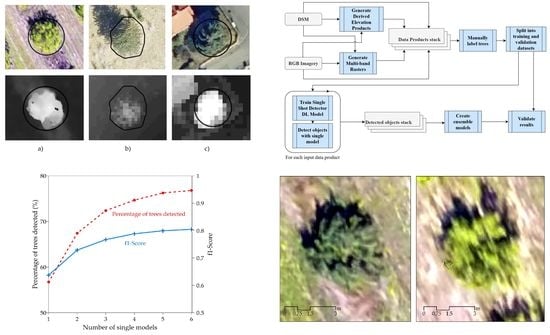
2.2.1. Overview

The flowchart of the deep learning tree-detection workflow is shown in Figure 2. First, a series of derived remote sensing products were generated from the RGB orthophoto and DSM using the ArcGIS 10.8 software (Figure 2—P1.1). Then, in addition to the derived products, we also generated two multi-band rasters which combine DSM and RGB information (Figure 2—P1.2). A data products stack (

Table 1. Remote sensing data products and spatial resolution for each study site. Original product column indicates the source datasets. Input product column describes the input products for single shot detector (SSD) models. Combinations are single file three-band rasters from the input products described.

Original Product	Input Product	Site 1	Site 2	Site 3
RGB	RGB	6 cm	12 cm	20 cm
	Grayscale	6 cm	12 cm	20 cm
	Principal Component Analysis (PCA)	6 cm	12 cm	20 cm
DSM	Digital Surface Model (DSM)	10 cm	100 cm	100 cm
	Canopy Height Model (CHM)	10 cm	100 cm	100 cm
	Slope	10 cm	100 cm	100 cm
	Hillshade	10 cm	100 cm	100 cm
	Box Cox	25 cm	100 cm	100 cm
Combinations	DSM–Slope–Hillshade	10 cm	100 cm	100 cm
	Grayscale–DSM–Slope	10 cm	100 cm	100 cm

) was obtained from the DSM and RGB input data products.

Trees were manually digitized for each site, and labels with species information were assigned to the polygons in order to create a tree label database (Figure 2—P2.1). Each tree label dataset was further split randomly into training and validation sets (Figure 2—P2.2). Single shot detector (SSD) models were then trained using the training dataset with the same model parameters (Figure 2—P3). Next, ensemble models were created by combining results from multiple SSD models (Figure 2—P4, P5). Finally, single models, as well as ensemble models, were validated using the validation set (Figure 2—P6).

2.2.2. Data Pre-Processing

As stated above, the RGB orthophotos and DSMs were used to derive six additional data products used to train the SSD models (Figure 2—P1.1). From the RGB data, two products were derived: a grayscale image and the first component of Principal Components Analysis (PCA) [37], at the same spatial resolution. Four main products were derived from the DSM: slope, slope normalized for frequency distribution, hillshade and Canopy Height Model (CHM). Slope and hillshade were derived in a standard approach as implemented in ArcGIS/Spatial Analyst version 10.8. The distribution of slope values is typically skewed, so the statistical analysis of the slope layer is often biased [38]. Thus, an additional layer was derived, consisting of slope normalized to frequency distribution by the Box Cox transformation using a tool developed by the authors of [38]. CHM was derived by subtracting the digital terrain model from the DSM.

In addition to the six derived data products, two three-band rasters were generated with the following layers as bands: Grayscale–DSM–Slope and DSM–Slope–Hillshade, with a spatial resolution equal to that of the DSM (Figure 2—P1.2). In total, the input data products stack consists of 10 rasters, which were used to train separate single shot detector deep learning models with identical parameters.

2.2.3. Preparing the Training and Validation Data

For each site, scattered trees were manually digitized and labeled with species information (Figure 2—P2.1). Understory trees were not digitized, as they are only present in site 2 and the RGB imagery is of not sufficient resolution for this task. In site 1, all the trees from the plot were digitized, as some of them were available from a field campaign. Each dataset of field trees was randomly split into 80% training and 20% validation (Figure 2—P2.2).

Table 2. Digitized tree labels for the deep learning models.

Site	Site 1			Site 2		Site 3
Species	Apricot	Plum	Walnut	Coniferous	Deciduous	No Species
Training Labels	1420	2354	634	1500	1250	1200
Validation Labels	356	589	159	300	250	300
Total Labels	1776	2493	793	1800	1500	1500

describes the number of labels used for training and validation.

2.2.4. Training Single Shot Detector Deep Learning Models

Image chips of the labeled tree locations were exported using ArcGIS API for Python (Figure 3). In order to reduce the risk of overfitting, data augmentation was used to boost the number of training chips to the order of tens of thousands. Augmentation included sample rotation at different angles and stride shift with a 50% overlap, thus obtaining additional subsets from the main chip image. The resulting image chips were rectangular subsets clipped from the input raster data and had different sizes according to the spatial resolution of the rasters, which differs between RGB and DSM.

Next, SSD deep learning models were trained using ArcGIS API for Python (Figure 2—P3). The SSD (Figure 4) is implemented in the API using the Fast.AI [39] and PyTorch [40] frameworks for deep learning. SSD has high speed and accuracy due to the use of multiple boxes of different sizes and an aspect ratio for detecting features. Predictions from multiple feature maps of different resolutions are combined to handle objects of various sizes [35]. The training of SSD was done using ResNet-152 architecture [41] from Torchvision version 0.3.0 [42].

To further reduce overfitting, in addition to data augmentation, early stopping was used for all models, which stopped the training if the validation loss did not improve for 5 epochs. The full model architecture with all parameters and layers is presented in Appendix A.

2.2.5. Detecting with Single Models

The trained SSD individual models on the ten input data products were used to predict tree locations and species in the three chosen sites. For each data product, multiple rectangular bounding boxes around predicted trees were obtained (Figure 2—P4), each bounding box having a confidence score ranging from 0 to 1, which indicates the degree of certitude for the presence of a tree. Afterwards, a non-maximum suppression algorithm [44] was used to remove the redundant bounding boxes that overlapped, by keeping the one with the highest confidence score. Finally, all bounding boxes with a confidence score < 0.2 were removed, thus retaining the best bounding box candidates to validate the detection algorithm.

The validation samples, along with the predicted tree bounding boxes, were used to compute the intersection-over-union statistic (IoU). IoU is a geometrical statistic which measures the area of the intersection divided by the area of overlap of the ground truth bounding box and the predicted bounding box. This indicator is very commonly used for the validation of deep learning object detection models, and an IoU > 0.5 is generally accepted as a proper threshold for a successful detection [21,32,45,46]. An IoU > 0.5 was the threshold to select the bounding boxes that were further statistically processed to assess the detection performance. The validation statistics used in reporting the results are the detection percentage and the f1-Score diagnostic [47], all computed using the metrics of recall and precision. Equations (1)–(5) describe the validation statistics used for validations:

$$\mathrm{Precision}=\frac{{\mathrm{T}}_{\mathrm{P}}}{{\mathrm{T}}_{\mathrm{P}}+{\mathrm{F}}_{\mathrm{P}}}$$

(1)

$$\mathrm{Recall}=\frac{{\mathrm{T}}_{\mathrm{P}}}{{\mathrm{T}}_{\mathrm{P}}+{\mathrm{F}}_{\mathrm{N}}}$$

(2)

$${\mathrm{f}1}_{\mathrm{species}}=\frac{2\times (\mathrm{Precision}\times \mathrm{Recall})}{\mathrm{Precision}+\mathrm{Recall}}$$

(3)

$$\mathrm{f}1-\mathrm{Score}={{\displaystyle \sum }}^{}{\mathrm{f}1}_{\mathrm{n}}{*\mathrm{w}}_{\mathrm{n}}$$

(4)

$$\mathrm{Detection}\mathrm{percentage}=\frac{{\mathrm{T}}_{\mathrm{P}}}{{\mathrm{T}}_{\mathrm{S}}}*100$$

(5)

T_P (true positive) indicates the number of trees successfully detected, F_P (false positive) denotes the number of objects incorrectly detected as trees; F_N indicates the number of trees not detected; f1_n indicates the f1-Score computed for a certain species; w_n indicates the weights attributed for each species and T_S denotes the total number of trees used for validation. The weights used for computing the overall f1-Score are according to the number of validation samples per species. The f1-Score (Equation (3)) was used to assess the performance of species classification; therefore, it was only computed for sites 1 and 2, where species information was available. Due to the class imbalance between species, a modified f1-Score (Equation (4)) implemented in the Scikit-learn package [48] was used when reporting the f1-Score for the overall performance of a model, regardless of species.

2.2.6. Ensemble Learning

The ensemble models were created from bounding box outputs of the single models (Figure 2—P5). The bounding boxes predicted by the single models were stacked together in different input data product combinations (see Figure 2).

Ensemble models were created by handling the ten input data products as a mathematical set. Using a mathematical combination, a number of 1023 unique k-combinations, excluding the empty set, were obtained. In order to reduce data redundancy and improve the variation, the combinations with duplicate input information were excluded. The duplicate information consists of the cases where any of the data product combinations described in

Table 3. Invalid input product pairs for the ensemble models.

Invalid Product Pairs
DSM/DSM–Slope–Hillshade
DSM/Grayscale–DSM–Slope
Slope/DSM–Slope–Hillshade
Slope/Grayscale–DSM–Slope
Hillshade/DSM–Slope–Hillshade
Grayscale/Grayscale–DSM–Slope
DSM–Slope–Hillshade/Grayscale–DSM–Slope
RGB/Grayscale–DSM–Slope
RGB/Grayscale
RGB/PCA
PCA/Grayscale
PCA/Grayscale–DSM–Slope

appear in a set. In this manner, the number of possible combinations was reduced to 150.

Using the validation dataset, each ensemble model was first validated for tree detection by applying a veto rule and a threshold IoU > 0.5. The veto rule is implemented for tree detection only and accepts all single input predictions, counting a correct tree detection if at least one single model part of the ensemble reaches IoU > 0.5. Secondly, for species identification, a voting strategy [49] was implemented. In this voting strategy, each single SSD model that was part of an ensemble which correctly identifies a tree was treated as binarized output (true/false). For each ensemble model, an array was constructed which contained true/false tree detection values, as well as tree species information corresponding to each single SSD model in the ensemble.

Then, a voting algorithm takes the output array of an ensemble and decides on the species detected. We tested four voting strategies, as follows:

• Majority: the majority of single models must agree the output species detected;
• Unison: all single models must agree the output species detected;
• Confidence: the model gives the output species with the highest SSD confidence value;
• Weighted: the output species is given by a weighted sum that applies weights based on the single models’ accuracy in terms of the f1-Score.

The ensemble models’ validation results by the voting strategies were ultimately statistically processed (Figure 2—P6) to estimate the detection performance by using the same indicators presented in Section 2.2.5 for single models.

3. Results

3.1. Single Product Models

As seen in

Table 4. Single models’ overall detection percentage on each of the three sites. The overall detection percentage does not take into account species variation.

Product	Detection Percentage—Site 1	Detection Percentage—Site 2	Detection Percentage—Site 3
RGB	21.61%	64.73%	73%
Grayscale	27.56%	38.55%	60.33%
PCA	27.87%	37.45%	38%
DSM	20.03%	0%	15.67%
Hillshade	28.17%	17.27%	14%
CHM	27.32%	24.36%	12.33%
Slope	25.63%	22%	10.67%
Box Cox	56.73%	21.82%	12%
Grayscale–DSM–Slope	1%	4.73%	1.33%
DSM–Slope–Hillshade	24.71%	14.36%	0.67%

, the overall detection rates were below 50%, yet with the notable exceptions of RGB in site 2 (detection percentage 64.73%) and site 3 (detection percentage 73%); Grayscale, with a detection percentage of 60.33% in site 3 and Box Cox in site 1, with a 56.7% detection.

However, the detection varies by species. For example, in site 1 (Figure 5), the walnut detection values are much higher (20–30% higher) than other species in almost all products except for Box Cox. In site 2 (Figure 6), the coniferous species has a slightly higher detection percentage (5–10% higher) for all products except RGB and DSM–Slope–Hillshade.

F1-Scores are presented in Figure 7 for sites 1 and 2. The highest f1-Score are 0.64 for Box Cox in site 1 and 0.78 for RGB in site 2. The single models trained on DSM and Grayscale–DSM–Slope performed poorly, with f1-Scores of 0.3 and 0 in site 1 and ~0.05 in site 2.

The variation between species manifests a more significant discrepancy as observed in terms of accuracy for site 1 (Figure 8a). Walnut trees reach a maximum of 0.76 f1-Score in grayscale and much higher values for the other products except for Box Cox. Plum trees have the lowest accuracy, with f1-Score values consistently below 0.4, except for Box Cox, where they reach the value of 0.7. In site 2 (Figure 8b), the coniferous and deciduous trees have roughly the same f1-Score in RGB, while for the rest of the models, the deciduous species have a lower accuracy by a margin of 0.1–0.2, except for DSM–Slope–Hillshade.

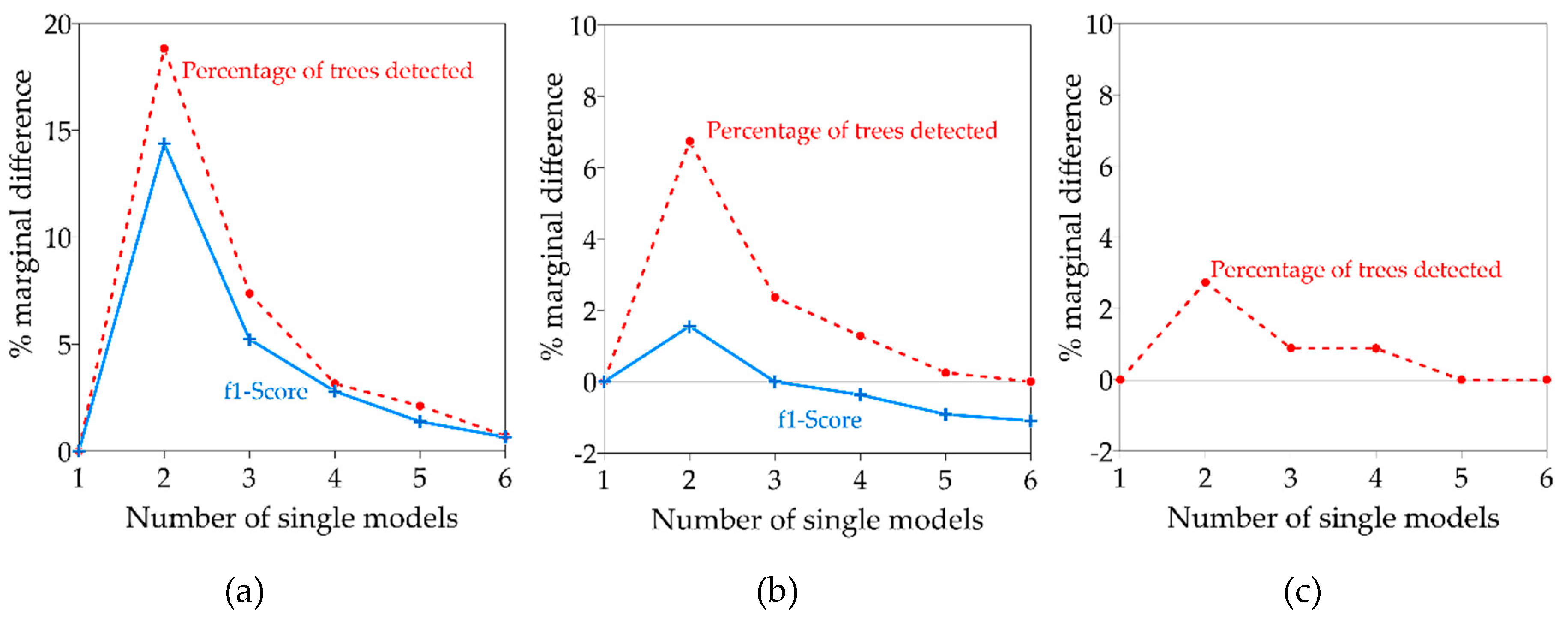
3.2. Ensemble Models

The ensemble models reached overall detection values of over 70% in all sites (

Table 5. Best performing ensemble models in terms of % overall tree detection in each site, based on majority voting strategy. If two ensemble models had the same detection percentage, the one reported was with the least number of individual single models.

Site	Ensemble Model	Detection Percentage
Site 1	DSM + Slope + Hillshade + PCA + Box Cox + CHM	76.8%
	DSM + Slope + Hillshade + Grayscale + Box Cox + CHM	76.43%
	Slope + Hillshade + PCA + Box Cox + CHM	76.25%
	Slope + Hillshade + Grayscale + Box Cox + CHM	76%
Site 2	RGB + Slope + Hillshade + Box Cox + CHM	71.82%
	RGB + Slope + Hillshade + CHM	71.64%
	RGB + Hillshade + Box Cox + CHM	71.45%
	RGB + DSM-Slope-Hillshade + Box Cox + CHM	71.27%
Site 3	RGB + DSM + Slope + CHM	76.33%
	RGB + DSM + Slope + Hillshade + CHM	76.33%
	RGB + DSM + Slope + Hillshade + Box Cox + CHM	76.33%
	RGB + DSM + Slope + Box Cox + CHM	76.33%

). In site 1, the highest detection rate reached 76.8% with the combination of DSM + Slope + Hillshade + PCA + Box Cox + CHM. The other combinations reached nearly the same detection percentage, with differences of 0.2–0.8%. In site 2, the highest detection percentage is 71.82%, reached equally by the first two models. The next two models have only a ~0.2% detection reduction. In site 3, the first four models all reach a maximum detection percentage of 76.33%.

Regarding species differences,

Table 6. Detection percentage per species and voting strategy of the best performing ensemble models in terms of % of trees detected (Det. per. %) in sites 1 and 2. If two ensemble models had the same detection percentage, the one reported was with the least number of individual single models.

Site	Species	Voting Strategy
		Majority		Unison		Weighted		Confidence
		Ensemble Model	Det. per. (%)	Ensemble Model	Det. per. (%)	Ensemble Model	Det. per. (%)	Ensemble Model	Det. per. (%)
Site 1	Plum	DSM + Slope + Hillshade + PCA + Box Cox + CHM	71.52	DSM + Slope + Hillshade + PCA + Box Cox + CHM	67.62	DSM + Slope + Hillshade + PCA + Box Cox + CHM	70.88	DSM + Slope + Hillshade + PCA + Box Cox + CHM	70.47
	Apricot	RGB + DSM + Slope + Hillshade + Box Cox + CHM	64.58	RGB + DSM + Slope + Hillshade + Box Cox + CHM	59.68	DSM + Slope + Hillshade + Grayscale + Box Cox + CHM	63.12	RGB + DSM + Slope + Hillshade + Box Cox + CHM	62.73
	Walnut	DSM + Slope + Hillshade + Grayscale + CHM	89.66	DSM + Slope + Hillshade + Grayscale + CHM	88.27	DSM + Slope + Hillshade + Grayscale + Box Cox + CHM	90.29	DSM + Slope + Hillshade + PCA + Box Cox + CHM	90.04
Site 2	Coniferous	RGB + Hillshade + CHM	67.00	RGB + Hillshade	66.00	RGB + Hillshade + CHM	67.33	RGB + Hillshade + CHM	67.67
	Deciduous	RGB + DSM–Slope–Hillshade + CHM	71.2	RGB + DSM–Slope–Hillshade	69.60	RGB + DSM–Slope–Hillshade + Box Cox + CHM	72.00	RGB + DSM–Slope–Hillshade + Box Cox + CHM	71.60

and

Table 7. Detection performance per species and voting strategy of the best ensemble models in terms of f1-Score (f1-S.) in sites 1 and 2. If two ensemble models had the same f1-Score, the one reported was with the least number of individual single models.

Site	Species	Voting Strategy
		Majority		Unison		Weighted		Confidence
		Ensemble Model	f1-S.	Ensemble Model	f1-S.	Ensemble Model	f1-S.	Ensemble Model	f1-S.
Site 1	Plum	DSM + Slope + Hillshade + PCA + Box Cox + CHM	0.814	DSM + Slope + Hillshade + PCA + Box Cox + CHM	0.793	DSM + Slope + Hillshade + PCA + Box Cox + CHM	0.809	DSM + Slope + Hillshade + PCA + Box Cox + CHM	0.806
	Apricot	RGB + DSM + Slope + Hillshade + Box Cox + CHM	0.766	RGB + DSM + Slope + Hillshade + Box Cox + CHM	0.736	RGB + DSM + Slope + Hillshade + Box Cox + CHM	0.750	RGB + DSM + Slope + Hillshade + Box Cox + CHM	0.747
	Walnut	DSM + Slope + Hillshade + Grayscale + CHM	0.925	Slope + Hillshade + Grayscale + CHM	0.921	DSM + Slope + Hillshade + Grayscale + CHM	0.922	DSM + Hillshade + Grayscale + CHM	0.920
Site 2	Coniferous	RGB + CHM	0.786	RGB + CHM	0.782	RGB + CHM	0.792	RGB + Slope + CHM	0.791
	Deciduous	RGB + DSM–Slope–Hillshade + CHM	0.809	RGB + DSM–Slope–Hillshade	0.813	RGB + DSM–Slope–Hillshade + Box Cox + CHM	0.828	RGB + DSM–Slope–Hillshade + Box Cox + CHM	0.821

summarize the detection percentages and f1-Scores for the top best performing ensemble model in each of the two sites.

In site 1, walnut species has the best detection accuracy of over 90.29% for the weighted method on the combination of DSM + Slope + Hillshade + Grayscale + Box Cox + CHM and also the best f1-Score of 0.925 for the majority method on the combination of DSM + Slope + Hillshade + Grayscale + CHM. The plum and apricot species have similar detection values and f1-Scores, at around 59–71% and 0.73–0.82%, respectively, with apricot slightly underperforming.

For each site, a frequency evaluation of each input data product for the top 15% of the ensemble models was also performed based on f1-Scores for sites 1 and 2 and percentage of trees detected for site 3. All results are summarized in

Table 8. Frequency (counts) of each input data product in the top 15% of ensemble models in terms of f1-Score in sites 1 and 2 and detection percentage in site 3. The counts are grouped by the voting method, if applied.

Input Data Product	Site 1				Site 2				Site 3
	Majority	Unison	Weighted	Confidence	Majority	Unison	Weighted	Confidence	No Voting
RGB	6	8	6	7	22	22	22	22	22
Grayscale	9	7	8	7	0	0	0	0	0
PCA	7	6	8	8	0	0	0	0	0
DSM	13	13	13	13	9	10	9	9	16
Hillshade	17	19	18	19	2	4	8	6	12
CHM	19	18	18	17	12	8	18	16	12
Slope	16	17	17	17	10	10	10	12	14
Box Cox	23	23	23	23	10	9	12	12	11
Grayscale–DSM–Slope	0	0	0	0	0	0	0	0	0
DSM–Slope–Hillshade	1	0	0	0	4	2	4	4	0

. The most heavily present input data products are Box Cox in site 1, with a count of 23 across all voting methods, and RGB in sites 2 and 3, with 22 counts for all voting methods. Other input data products such as CHM, Hillshade, Slope and DSM are also frequent in all sites. Some models have very low or no contribution to ensemble models, such as the three-band rasters Grayscale–DSM–Slope and DSM–Slope–Hillshade.

We next investigated whether there is a relationship between the number of input data products in an ensemble model and the detection percentage or accuracy of the model. In Figure 9, the maximum detection percentage and f1-Score were plotted against the number of single models in an ensemble model.

For both sites, it is observed that combining single models in an ensemble model generally increases the detection percentage and, to a lesser degree, the f1-Score. Furthermore, by looking at the percentage difference in detection performance or f1-Score when adding a new single model into an ensemble model, it can be observed (Figure 10) that the maximum increase for both indicators is reached when adding just one more single model.

For example, an increase of 18.8% in detection performance and a 14.3% increase in f1-Score were recorded for site 1. Sites 2 and 3 follow a similar trend but with slightly lower values: a 6.74% increase in detection performance and 1.5% increase in f1-Score in site 2 and a 2.7% increase in detection performance in site 3. Continuously adding new single models into an ensemble model leads to a rapid reduction in the accuracy parameters or even a decrease in f1-Score, as observed in site 2. The same relationship between the number of ensemble models and indicators of model performance is observed in all sites, although at different scales.

4. Discussion

4.1. Single vs. Ensemble Models

Designing an ensemble with only two single models increased the detection accuracy by a large margin of 3–18%. Adding more single models further increased the performance, but in a slower measure, or even actually decreasing the accuracy. This effect has also been observed in [17] and [18], for certain species in terms of detection performance in similar remote sensing imagery, and can be attributed to subtle spectral differences between species, other small-scale effects which are not captured by the deep learning algorithm. Another explanation could be that increasing the number of combined models to form an ensemble decreases the error independence between the single models. Although interspecies differences are present, the overall performance and effects of ensemble models are common in all sites (Figure 10) and clearly show superior efficiency. This validates and strengthens the general findings [31] that ensemble neural networks are superior to single ones in terms of accuracy, not only in the context of non-geospatial data but also in applications that deal with high-resolution remote sensing data. Studies which designed and tested ensemble models with remote sensing data reported analogous outcomes, albeit with different ensemble model designs. For example, in object detection tasks, the authors of [17] proposed an ensemble model by fusing hyperspectral imagery and LiDAR data for tree-crown detection, a model that resulted in superior accuracy to single trained models by a margin of 5–15%; the authors of [32] designed an ensemble model for object detection in remote sensing imagery at different scales, which outperformed most traditional CNNs in terms of accuracy by 5–10%, especially for densely packed objects; the authors of [18] implemented a fusion of remote sensing imagery and LiDAR information in the training data space of a dense convolutional network, achieving superior accuracy for tree detection in an urban environment by a margin of 5%-10% than single product trained models. Ensemble models used for remote sensing imagery classification report analogous results. For instance, the authors of [33] designed a similar voting strategy ensemble for the classification of remote sensing imagery, which resulted in substantially better performance over single models, within a statistical significance of over 95%. In [50] an ensemble model fusing two CNN architectures for land classification using remote sensing data achieved an accuracy of up to 4% higher to that of the single CNN models tested; the authors of [51] implemented a cascade ensemble from hyperspectral imagery and LiDAR data that outperformed traditional CNN-based methods in a classification task by a factor of 4–8%. On account of all the above, we conclude that ensemble models’ performance surpassed the single product trained models by a large margin in terms of detection percentage as well as accuracy.

4.2. Input Data Products Performance vs. Image Resolution

The input data products, including the derived ones, manifested variation in terms of performance by species and site. Table 8 presents the frequency of input data products in the top 15% best performing ensemble models. RGB is the most frequent in sites 2 and 3, as it appears 22 times, while in site 1, it appears only 6–8 times. Sites 2 and 3 have similar pixel sizes of 12 cm and 20 cm, respectively, while site 1 has a 6-cm spatial resolution. In site 1, due to the ultra-high spatial resolution, the spectral information of objects is rich. Consequently, the discrimination between species is hindered, especially between plum and apricot species, which, on visual interpretation of the imagery data, appear almost structurally and spectrally indistinguishable (Figure 11). Therefore, the difference between species is made by adding data derived from DSM, namely Box Cox, which is present 23 times, followed by CHM, Hillshade and Slope with frequencies of 17–19 times. The DSM and CHM performances for this site are roughly the same in terms of overall detection percentage (Table 4) and contribution to ensemble models (Table 8). The same effect is observed in site 3, which has a similar, relatively flat topography. This seems to show that in flat topography, the DSM and CHM information have largely the same importance for individual tree-crown detection.

In site 2, on the other hand, the difference between species is made primarily by the RGB information. As seen in Table 4, the DSM has no detection as a single model, a fact which might be due to the significant differences in elevation values between trees. The detrimental effect of DSM on tree detection in uneven terrain has also been shown in [52]. However, the coniferous and deciduous trees have clear spectral and structural differences, information which drives the distinction between these species. With counts of 22 for RGB, compared to 10–12 for DSM and other derivatives, the advantage of RGB in this context is straightforward.

The influence of canopy cover on tree detection accuracy has not been evaluated. In a recent study [53], different tree-crown detection algorithms were assessed under various canopy cover conditions and a reduction in accuracy directly related to an increase in canopy cover rate was reported. However, the authors report a high dependency on spatial resolution of the tree detection methods and did not employ deep learning techniques. Given the large diversity of spatial features between our sites and the objectively good results for tree-crown detection across image resolutions, we can uphold the idea that the ensemble model examples are robust enough to deal with forested sites that have a high rate of canopy cover. The risk of overfitting is greatly reduced by data augmentation and the early stopping procedure. In addition, the ensemble models are designed to reduce information duplication which can lead to overfitting, by removing invalid combinations (Table 4).

4.3. Performance of Voting Strategies

In sites 1 and 2, we tested the performance of the voting strategies for species discrimination. Table 6 and Table 7 summarize the detection percentages and f1-Scores for each species and voting strategy. In site 1, the majority strategy outperforms the other three by 1–5%, in the case of plum and apricot species, while the weighted strategy performs better for walnut. In site 2, the weighted strategy surpassed the other ones in nearly all cases by a margin of 1–3%. In a study [54] which tested two box voting strategies for ensemble models, an accuracy difference of 2% was found, which is similar to our results. The different results between voting strategies, while small at first glance, are actually indicative of slight divergences of the voting design, which can be exploited in order to satisfy the various objectives of an object detection task with ensemble models. In detail, they can be used to balance between precision and recall metrics in order to accomplish the detection objective better. For example, in

Table 9. Average precision and recall values by voting strategy in sites 1 and 2. The average is calculated from the top 20 best performing ensemble models in terms of f1-Score.

Voting Strategy	Site 1		Site 2
	Precision	Recall	Precision	Recall
Majority	0.93	0.7	0.96	0.66
Unison	0.95	0.66	0.98	0.63
Weighted	0.92	0.69	0.97	0.68
Confidence	0.92	0.69	0.97	0.68

, the unison strategy, which only accepts as correct when all models part of the ensemble give the same result, yields the highest precision in all sites and at the same time has the lowest recall.

For an ensemble model which needs to maximize precision, the unison voting strategy may be used. In reverse, if a model needs to have a good recall—that is, to find as many objects as possible while still maintaining good precision—a weighted or a confidence strategy may be used.

5. Conclusions

In this article, an ensemble deep learning design based on a single shot detector (SSD) model was developed for individual tree-crown detection and species classification, based on very high-resolution remote sensing data. The design was tested in disparate study sites in terms of spatial pattern. Results have shown the increased performance of ensemble models compared to single ones by a margin of 3%-18%. RGB information was found to be the most important factor influencing the species identification. DSM derived data were shown to have significant importance in species discrimination, especially in the structurally complex site 1, where RGB trained models performed poorly. Lastly, the voting strategies for combining the outputs allowed us to better tune the ensemble models in order to accommodate specific detection objectives. Due to the common effects observed for the ensemble models, our design proposal has been shown to have notable transferability capabilities across disparate tree conditions. Further research is necessary in order to investigate more complex data derivates from RGB and DSM in addition to those presented in this study.

References

1. Zhen, Z.; Quackenbush, L.J.; Zhang, L. Trends in automatic individual tree crown detection and delineation-evolution of LiDAR data. Remote Sens. 2016, 8, 333. [Google Scholar] [CrossRef] [Green Version]
2. Ke, Y.; Quackenbush, L.J. A review of methods for automatic individual tree-crown detection and delineation from passive remote sensing. Int. J. Remote Sens. 2011, 32, 4725–4747. [Google Scholar] [CrossRef]
3. Disney, M. Terrestrial LiDAR: A three-dimensional revolution in how we look at trees. New Phytol. 2019, 222, 1736–1741. [Google Scholar] [CrossRef] [Green Version]
4. Clark, M.L.; Roberts, D.A.; Clark, D.B. Hyperspectral discrimination of tropical rain forest tree species at leaf to crown scales. Remote Sens. Environ. 2005, 96, 375–398. [Google Scholar] [CrossRef]
5. Williams, J.; Schonlieb, C.B.; Swinfield, T.; Lee, J.; Cai, X.; Qie, L.; Coomes, D.A. 3D Segmentation of Trees through a Flexible Multiclass Graph Cut Algorithm. IEEE Trans. Geosci. Remote Sens. 2019, 58, 754–776. [Google Scholar] [CrossRef]
6. White, J.C.; Wulder, M.A.; Vastaranta, M.; Coops, N.C.; Pitt, D.; Woods, M. The utility of image-based point clouds for forest inventory: A comparison with airborne laser scanning. Forests 2013, 4, 518–536. [Google Scholar] [CrossRef] [Green Version]
7. Goodbody, T.R.H.; Coops, N.C.; White, J.C. Digital Aerial Photogrammetry for Updating Area-Based Forest Inventories: A Review of Opportunities, Challenges, and Future Directions. Curr. For. Rep. 2019, 5, 55–75. [Google Scholar] [CrossRef] [Green Version]
8. Iglhaut, J.; Cabo, C.; Puliti, S.; Piermattei, L.; O’Connor, J.; Rosette, J. Structure from Motion Photogrammetry in Forestry: A Review. Curr. For. Rep. 2019, 5, 155–168. [Google Scholar] [CrossRef] [Green Version]
9. Larsen, M.; Eriksson, M.; Descombes, X.; Perrin, G.; Brandtberg, T.; Gougeon, F.A. Comparison of six individual tree crown detection algorithms evaluated under varying forest conditions. Int. J. Remote Sens. 2011, 32, 5827–5852. [Google Scholar] [CrossRef]
10. Hamraz, H.; Contreras, M.A.; Zhang, J. Forest understory trees can be segmented accurately within sufficiently dense airborne laser scanning point clouds. Sci. Rep. 2017, 7, 6770. [Google Scholar] [CrossRef] [Green Version]
11. Li, L.; Chen, J.; Mu, X.; Li, W.; Yan, G.; Xie, D.; Zhang, W. Quantifying Understory and Overstory Vegetation Cover Using UAV-Based RGB Imagery in Forest Plantation. Remote Sens. 2020, 12, 298. [Google Scholar] [CrossRef] [Green Version]
12. Chianucci, F.; Cutini, A.; Corona, P.; Puletti, N. Estimation of leaf area index in understory deciduous trees using digital photography. Agric. For. Meteorol. 2014, 198, 259–264. [Google Scholar] [CrossRef] [Green Version]
13. Ma, L.; Liu, Y.; Zhang, X.; Ye, Y.; Yin, G.; Johnson, B.A. Deep learning in remote sensing applications: A meta-analysis and review. ISPRS J. Photogramm. Remote Sens. 2019, 152, 166–177. [Google Scholar] [CrossRef]
14. Guan, H.; Yu, Y.; Ji, Z.; Li, J.; Zhang, Q. Deep learning-based tree classification using mobile LiDAR data. Remote Sens. Lett. 2015, 6, 864–873. [Google Scholar] [CrossRef]
15. Zou, X.; Cheng, M.; Wang, C.; Xia, Y.; Li, J. Tree Classification in Complex Forest Point Clouds Based on Deep Learning. IEEE Geosci. Remote Sens. Lett. 2017, 14, 2360–2364. [Google Scholar] [CrossRef]
16. Li, W.; Fu, H.; Yu, L.; Cracknell, A. Deep Learning Based Oil Palm Tree Detection and Counting for High-Resolution Remote Sensing Images. Remote Sens. 2017, 9, 22. [Google Scholar] [CrossRef] [Green Version]
17. Liao, W.; Van Coillie, F.; Gao, L.; Li, L.; Zhang, B.; Chanussot, J. Deep Learning for Fusion of APEX Hyperspectral and Full-Waveform LiDAR Remote Sensing Data for Tree Species Mapping. IEEE Access 2018, 6, 68716–68729. [Google Scholar] [CrossRef]
18. Hartling, S.; Sagan, V.; Sidike, P.; Maimaitijiang, M.; Carron, J. Urban tree species classification using a worldview-2/3 and liDAR data fusion approach and deep learning. Sensors 2019, 19, 1284. [Google Scholar] [CrossRef] [PubMed] [Green Version]
19. Tianyang, D.; Jian, Z.; Sibin, G.; Ying, S.; Jing, F. Single-Tree Detection in High-Resolution Remote-Sensing Images Based on a Cascade Neural Network. ISPRS Int. J. Geo-Inf. 2018, 7, 367. [Google Scholar] [CrossRef] [Green Version]
20. Safonova, A.; Tabik, S.; Alcaraz-Segura, D.; Rubtsov, A.; Maglinets, Y.; Herrera, F. Detection of Fir Trees (Abies sibirica) Damaged by the Bark Beetle in Unmanned Aerial Vehicle Images with Deep Learning. Remote Sens. 2019, 11, 643. [Google Scholar] [CrossRef] [Green Version]
21. Weinstein, B.G.; Marconi, S.; Bohlman, S.A.; Zare, A.; White, E.P. Cross-site learning in deep learning RGB tree crown detection. Ecol. Inform. 2020, 56, 101061. [Google Scholar] [CrossRef]
22. Hamraz, H.; Jacobs, N.B.; Contreras, M.A.; Clark, C.H. Deep learning for conifer/deciduous classification of airborne LiDAR 3D point clouds representing individual trees. ISPRS J. Photogramm. Remote Sens. 2019, 158, 219–230. [Google Scholar] [CrossRef] [Green Version]
23. Opitz, D.; Maclin, R. Popular Ensemble Methods: An Empirical Study. J. Artif. Intell. Res. 1999, 11, 169–198. [Google Scholar] [CrossRef]
24. Polikar, R. Ensemble Learning. In Ensemble Machine Learning: Methods and Applications; Zhang, C., Ma, Y., Eds.; Springer: Boston, MA, USA, 2012; pp. 1–34. ISBN 978-1-4419-9326-7. [Google Scholar]
25. Michalski, R.S. A theory and methodology of inductive learning. In Machine Learning; Springer: Berlin, Heidelberg, 1983; pp. 83–134. [Google Scholar]
26. Hansen, L.K.; Salamon, P. Neural network ensembles. IEEE Trans. Pattern Anal. Mach. Intell. 1990, 12, 993–1001. [Google Scholar] [CrossRef] [Green Version]
27. Mandler, E.; Schümann, J. Combining the classification results of independent classifiers based on the Dempster/Shafer theory of evidence. In Machine Intelligence and Pattern Recognition; Elsevier: Amsterdam, The Netherlands, 1988; Volume 7, pp. 381–393. [Google Scholar]
28. Sharkey, A.J.C. On combining artificial neural nets. Conn. Sci. 1996, 8, 299–314. [Google Scholar] [CrossRef]
29. Cunningham, P.; Carney, J. Diversity versus Quality in Classification Ensembles Based on Feature Selection BT—Machine Learning: ECML 2000; López de Mántaras, R., Plaza, E., Eds.; Springer: Berlin/Heidelberg, Germany, 2000; pp. 109–116. [Google Scholar]
30. Krogh, A.; Vedelsby, J. Neural network ensembles, cross validation, and active learning. In Advances in Neural Information Processing Systems; MIT Press: Cambridge, MA, USA, 1995; pp. 231–238. [Google Scholar]
31. Battiti, R.; Colla, A.M. Democracy in neural nets: Voting schemes for classification. Neural Netw. 1994, 7, 691–707. [Google Scholar] [CrossRef]
32. Deng, Z.; Sun, H.; Zhou, S.; Zhao, J.; Lei, L.; Zou, H. Multi-scale object detection in remote sensing imagery with convolutional neural networks. ISPRS J. Photogramm. Remote Sens. 2018, 145, 3–22. [Google Scholar] [CrossRef]
33. Giacinto, G.; Roli, F.; Bruzzone, L. Combination of neural and statistical algorithms for supervised classification of remote-sensing images. Pattern Recognit. Lett. 2000, 21, 385–397. [Google Scholar] [CrossRef] [Green Version]
34. Partridge, D.; Yates, W.B. Engineering Multiversion Neural-Net Systems. Neural Comput. 1996, 8, 869–893. [Google Scholar] [CrossRef]
35. Liu, W.; Anguelov, D.; Erhan, D.; Szegedy, C.; Reed, S.; Fu, C.Y.; Berg, A.C. SSD: Single shot multibox detector. In Proceedings of the Lecture Notes in Computer Science (Including Subseries Lecture Notes in Artificial Intelligence and Lecture Notes in Bioinformatics); Springer: Cham, Switzerland, 2016; Volume 9905, pp. 21–37. [Google Scholar]
36. Thüringer Landesamt für Bodenmanagement und Geoinformation. Available online: https://www.geoportal-th.de/de-de (accessed on 12 December 2019).
37. Corner, B.R.; Narayanan, R.M.; Reichenbach, S.E. Principal component analysis of remote sensing imagery: Effects of additive and multiplicative noise. In Proceedings of the SPIE on Applications of Digital Image Processing XXII, Denver, CO, USA, 18–23 July 1999; Volume 3808, pp. 183–191. [Google Scholar]
38. Csillik, O.; Evans, I.S.; Drăguţ, L. Transformation (normalization) of slope gradient and surface curvatures, automated for statistical analyses from DEMs. Geomorphology 2015, 232, 65–77. [Google Scholar] [CrossRef]
39. Howard, J.; Gugger, S. Fastai: A Layered API for Deep Learning. Information 2020, 11, 108. [Google Scholar] [CrossRef] [Green Version]
40. Paszke, A.; Gross, S.; Massa, F.; Lerer, A.; Bradbury, J.; Chanan, G.; Killeen, T.; Lin, Z.; Gimelshein, N.; Antiga, L.; et al. PyTorch: An Imperative Style, High-Performance Deep Learning Library. In Proceedings of the Advances in Neural Information Processing Systems, Vancouver, BC, Banada, 8–14 December 2019; pp. 8024–8035. [Google Scholar]
41. He, K.; Zhang, X.; Ren, S.; Sun, J. Deep residual learning for image recognition. In Proceedings of the IEEE Computer Society Conference on Computer Vision and Pattern Recognition, Las Vegas, NV, USA, 27–30 June 2016; pp. 770–778. [Google Scholar] [CrossRef]
42. Marcel, S.; Rodriguez, Y. Torchvision the machine-vision package of torch. In Proceedings of the MM’10—ACM Multimedia 2010 International Conference, Philadelphia, PA, USA, 12–16 October 2010; ACM Press: New York, NY, USA, 2010; pp. 1485–1488. [Google Scholar]
43. Körez, A.; Barışçı, N.; Çetin, A.; Ergün, U. Weighted Ensemble Object Detection with Optimized Coefficients for Remote Sensing Images. ISPRS Int. J. Geo-Inf. 2020, 9, 370. [Google Scholar] [CrossRef]
44. Qiu, S.; Wen, G.; Deng, Z.; Liu, J.; Fan, Y. Accurate non-maximum suppression for object detection in high-resolution remote sensing images. Remote Sens. Lett. 2018, 9, 237–246. [Google Scholar] [CrossRef]
45. Tang, T.; Zhou, S.; Deng, Z.; Lei, L.; Zou, H. Arbitrary-Oriented Vehicle Detection in Aerial Imagery with Single Convolutional Neural Networks. Remote Sens. 2017, 9, 1170. [Google Scholar] [CrossRef] [Green Version]
46. Wu, X.; Sahoo, D.; Hoi, S.C.H. Recent advances in deep learning for object detection. Neurocomputing 2020. [Google Scholar] [CrossRef] [Green Version]
47. Powers, D. Evaluation: From Precision, Recall and F-Factor to ROC, Informedness, Markedness & Correlation. Mach. Learn. Technol. 2011, 2, 37–63. [Google Scholar]
48. Pedregosa, F.; Varoquaux, G.; Gramfort, A.; Michel, V.; Thirion, B.; Grisel, O.; Blondel, M.; Prettenhofer, P.; Weiss, R.; Dubourg, V.; et al. Scikit-learn: Machine Learning in {P}ython. J. Mach. Learn. Res. 2011, 12, 2825–2830. [Google Scholar]
49. Zhou, Z.-H. Ensemble Methods: Foundations and Algorithms; CRC Press: Boca Raton, FL, USA, 2012. [Google Scholar]
50. Minetto, R.; Segundo, M.P.; Sarkar, S. Hydra: An Ensemble of Convolutional Neural Networks for Geospatial Land Classification. IEEE Trans. Geosci. Remote Sens. 2018, 57, 6530–6541. [Google Scholar] [CrossRef] [Green Version]
51. Xu, X.; Li, W.; Ran, Q.; Du, Q.; Gao, L.; Zhang, B. Multisource Remote Sensing Data Classification Based on Convolutional Neural Network. IEEE Trans. Geosci. Remote Sens. 2018, 56, 937–949. [Google Scholar] [CrossRef]
52. Stupariu, M.-S.; Pleșoianu, A.-I.; Pătru-Stupariu, I.; Fürst, C. A Method for Tree Detection Based on Similarity with Geometric Shapes of 3D Geospatial Data. ISPRS Int. J. Geo-Inf. 2020, 9, 298. [Google Scholar] [CrossRef]
53. Peng, X.; Li, X.; Wang, C.; Zhu, J.; Liang, L.; Fu, H.; Du, Y.; Yang, Z.; Xie, Q. SPICE-based SAR tomography over forest areas using a small number of P-band airborne F-SAR images characterized by non-uniformly distributed baselines. Remote Sens. 2019, 11, 975. [Google Scholar] [CrossRef] [Green Version]
54. Lee, J.; Lee, S.-K.; Yang, S.-I. An ensemble method of cnn models for object detection. In Proceedings of the 2018 International Conference on Information and Communication Technology Convergence (ICTC), Jeju Island, Korea, 17–19 October 2018; pp. 898–901. [Google Scholar]
Figure 1. Study sites in Romania and Germany. Site 1 named Moara Domnească: orchard with trees of J. regia, P. armeniaca and P. domestica species; site 2 named Fundata: natural wooded pasture with P. abies, F. sylvatica and J. communis; site 3: city, named Erfurt, with no species information.
Remotesensing 12 02426 g001
Figure 2. The flowchart of the deep learning tree-crown detection method. Gray boxes indicate input and intermediary data products. Blue boxes indicate processing and analysis stages. The processing stages are labelled from P.1 to P.6.
Remotesensing 12 02426 g002
Figure 3. Example of training samples on RGB ortophoto (ac) and DSM (df) for (a,d) site 1; (b,e) site 2 and (c,f) site 3. The different resolution of input data is discernable between the three sites. The shape of the tree-crown polygon is irrelevant to the training process, as the exported image chips store the polygon geometry as extent coordinates, which always describe a rectangular shape.
Remotesensing 12 02426 g003
Figure 4. The single shot detector (SSD) architecture. The figure is adapted from [35] and [43]. The full parameters and layers of the SSD model that we used are available in Appendix A.
Remotesensing 12 02426 g004
Figure 5. The detection percentage grouped by species for single SSD models in site 1. Some models have fewer or no bars for species, indicating that they failed to detect any trees.
Remotesensing 12 02426 g005
Figure 6. The detection percentage grouped by species for single SSD models in site 2.
Remotesensing 12 02426 g006
Figure 7. F1-Scores of single product models in sites 1 and 2.
Remotesensing 12 02426 g007
Figure 8. Single models f1-Score by species in site 1 (a) and site 2 (b).
Remotesensing 12 02426 g008
Figure 9. Maximum percentage detection and f1-Score reached for each combination of 2..n number of models in sites 1 (a) and 2 (b).
Remotesensing 12 02426 g009
Figure 10. Marginal percentage difference in detection performance and f1-Score for each combination of 2..n number of models in all sites. Figure captions indicate individual study sites: (a) site 1, (b) site 2, (c) site 3.
Remotesensing 12 02426 g010
Figure 11. Spectral differences between apricot (a) and plum (b). Unmanned aerial vehicle (UAV) RGB imagery at 6-cm spatial resolution.
Remotesensing 12 02426 g011