Machine Learning for Cloud Detection of Globally Distributed Sentinel-2 Images

Abstract

In recent years, a number of different procedures have been proposed for segmentation of remote sensing images, basing on spectral information. Model-based and machine learning strategies have been investigated in several studies. This work presents a comprehensive overview and an unbiased comparison of the most adopted segmentation strategies: Support Vector Machines (SVM), Random Forests, Neural networks, Sen2Cor, FMask and MAJA. We used a training set for learning and two different independent sets for testing. The comparison accounted for 135 images acquired from 54 different worldwide sites. We observed that machine learning segmentations are extremely reliable when the training and test are homogeneous. SVM performed slightly better than other methods. In particular, when using heterogeneous test data, SVM remained the most accurate segmentation method while state-of-the-art model-based methods such as MAJA and FMask obtained better sensitivity and precision, respectively. Therefore, even if each method has its specific advantages and drawbacks, SVM resulted in a competitive option for remote sensing applications.

1. Introduction

Accurate land cover classification of multispectral remote sensing images is of paramount importance to fully exploit their informative content. The correct detection of clouds, shadows, snow or ice, is critical for many activities such as image compositing [1], correction for atmosphere effects [2,3], calculation of vegetation indices [4], classification of land cover [5] and change detection [6]. In recent years, different strategies have been proposed especially for cloud segmentation. In particular, two different strategies can be distinguished [7]: (i) model-based approaches, in this case pixels are assigned to a specific category by evaluating the available reflectances and using an a priori physical model to determine proper thresholds; (ii) learning approaches, these strategies exploit supervised algorithms to learn statistical models able to maximize the separation of pixels belonging to different classes and minimize classification errors.

Model-based approaches use specific physical constraints to separate different classes according to spectral bands; these constraints are usually formalized by proper combining the bands in suitable indicators and thresholds, which assign an image pixel or polygon to a class [2,8,9]. Accordingly, the implementation of model-based methods is computationally efficient and makes them particularly suitable for large scale satellite applications. However, especially when relying on hand-crafted features or empirical and study-specific thresholds, these methods may present some issues in segmenting particular classes such as low clouds and bright deserts [10,11]. A possible solution is considering models that include information from multiple time observations, namely multi-temporal approaches [12]; they exploit the information of several time points to approach cloud segmentation as a novelty detection problem. Of course, this solution requires increased computational requirements for both processing time and storage [12,13].

More recently, alternative strategies exploiting machine learning and deep learning have been proposed [14,15,16,17,18]. Learning strategies provide excellent segmentations for many applications such as the separation of clear-sky pixels from cloudy ones. This task is particularly challenging when relying only on spectral features [19], a possible reason being the difficulty in detecting thin clouds, which share a spectral signature similar to that of the underneath surface [5].

It is worth noting that in some cases machine learning can be computationally demanding and can require large training sets. However, the increasing availability of low-cost and high-performance computational infrastructures and the possibility for researchers to easily access different image databases has eased their adoption.

In this work we intend to investigate advantages and drawbacks of both approaches by comparing their segmentation performance using several metrics and data. Recently, a first study compared one learning method, based on boosting, with three model-based approaches on a dataset of Amazon forest images [20]. Here, we consider a larger and more heterogeneous dataset, including images from all over the world, and extend the comparison to six different methods.

The unbiased evaluation of segmentation algorithms is particularly compelling in medical applications, this is why in recent years many efforts have been devoted to the organization of “challenges” where different algorithms are trained on a common set and evaluated on an independent test set [21,22]. Accordingly, in this work we use three publicly available datasets of Sentinel-2 L1C images: a first dataset was used for training of machine learning methods; a second homogeneous dataset, characterized by the same segmentation protocols and similar geographical distribution, was used for validation and a first comparison with model-based segmentations; finally, a completely independent dataset was used as to evaluate segmentation performance when considering heterogeneous data.

2. Sentinel-2 Data

The Sentinel-2 mission provides multispectral observations with a spatial resolution up to 10 m and systematic global coverage of the Earth’s land surface. In particular, these data contain information from 13 different bands $Bx$, where x is a code identifying a band that captures specific land properties (see

Table 1. Sentinel-2 MSI spatial resolution, central wavelength and bandwidth.

Sentinel-2 Bands	Spatial Resolution (m)	Central Wavelength (nm)	Bandwidth (nm)
B1 – Coastal aerosol	60	442.7	21
B2 – Blue	10	492.4	66
B3 – Green	10	559.8	36
B4 – Red	10	664.6	31
B5 – Vegetation Red Edge	20	704.1	15
B6 – Vegetation Red Edge	20	740.5	15
B7 – Vegetation Red Edge	20	782.8	20
B8 – NIR	10	832.8	106
B8a – Narrow NIR	20	864.7	21
B9 – Water vapour	60	945.1	20
B10 – SWIR Cirrus	60	1373.5	31
B11 – SWIR	20	1613.7	91
B12 – SWIR	20	2202.4	175

).

Their central wavelength ranges from $442.7$ nm for $B1$ to $2202.4$ nm for $B12$. $B1$ is coastal aerosol, useful for imaging of shallow waters; $B2$, $B3$ and $B4$ are the blue, green and red bands, respectively; $B5$, $B6$ and $B7$ are useful for vegetation; $B8$ and $B8a$ are near infrared bands, suitable to measure plant health; $B9$ is water vapour band; $B10$, $B11$ and $B12$ are shortwave infrared (SWIR) bands, particularly useful for cirrus detection. Sentinel-2 data are available to users under a free and open data policy, which underpins the development of long-term, sustainable Earth Observation (EO) applications.

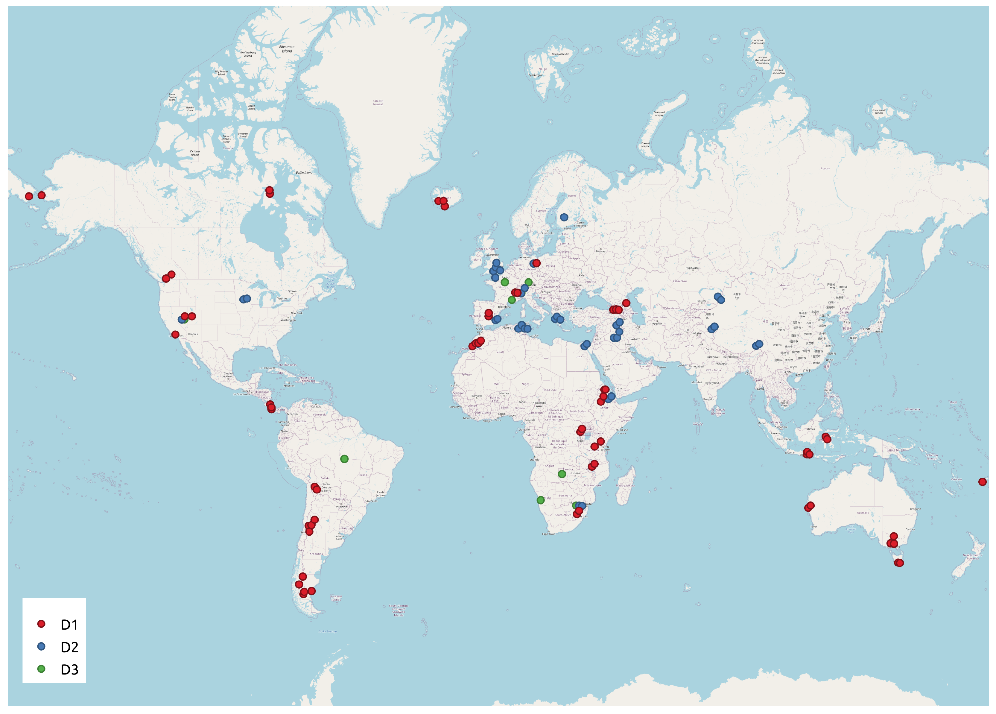
In this work we used three publicly available data sets of manually labelled Sentinel-2 scenes, the distribution of which is shown in Figure 1. We used the first set for training and tuning of machine learning models (Support Vector Machines, Random Forests and Neural Networks), the second and the third one for test and comparison on homogeneous and inhomogeneous data with the state-of-the-art model-based segmentations (Sen2Cor, FMask and MAJA). Further details about the segmentation methods will be provided in the next section.

The first dataset ${\mathcal{D}}_1$ consists of about $3.8$ million labelled pixels from 67 scenes and 26 different sites; according to the original works [23,24], pixels belong to six different classes:

• Water;
• Snow;
• Clouds;
• Cirrus;
• Clear sky;
• Shadows.

This dataset was selected to ensure a global geographical distribution and, therefore, a wide scene variability. This variability is highlighted in Figure 1.

The second set ${\mathcal{D}}_2$ consists of about $2.7$ million labelled pixels from 39 scenes and 18 sites. This set has been collected by the same authors of [23,24] and it is labelled according to the same labels of ${\mathcal{D}}_1$. The homogeneity of this data provides an excellent way to test the reliability of machine learning methods.

Finally, the third set ${\mathcal{D}}_3$ consists of about 100 million labelled pixels from 29 scenes [25,26] captured in 10 different sites. This set was used to test the generalization power of the machine learning methodologies across a non homogeneous set of images collected with different modalities and in different sites. ${\mathcal{D}}_3$ includes the following classes:

• Low cloud;
• High cloud;
• Cloud shadow;
• Land;
• Water;
• Snow.

As we are interested in detecting clouds, we regrouped them into clear sky and clouds. A synthetic overview about ${\mathcal{D}}_1$, ${\mathcal{D}}_2$ and ${\mathcal{D}}_3$ is provided in

Table 2. Overview of the data used in this work: ${\mathcal{D}}_1$ training, ${\mathcal{D}}_2$ homogeneous test, ${\mathcal{D}}_3$ inhomogeneous test.

Dataset	# Pixels	# Images	# Sites	Cloud Fraction	Spatial Resolution
${\mathcal{D}}_1$	3.87 ×${10}^6$	67	26	28%	20 m
${\mathcal{D}}_2$	2.73 ×${10}^6$	39	18	30%	20 m
${\mathcal{D}}_3$	8.24 ×${10}^7$	29	10	25%	60 m

.

Although Sentinel-2 cirrus band $B10$, centred at 1.38 $\mathsf{\mu }$m, was designed to detect high clouds, the only light reflected in this band comes from altitudes above 1000–2000 m [27]. Thus, in order to avoid misclassification of high altitude bright rocks, GTOPO30 digital elevation models were included in our analyses [28].

3. Model-Based Segmentation

Model-based methodologies consist of a series of constraints based on physical models and phenomenological observations. These constraints provide ranges and thresholds for reflectances and their ratios, which can be used to assign the image pixels to different classes [29]. Among several possibilities, we present here the evaluation and the comparison of the most adopted and accurate, according to recent literature, model-based segmentation algorithms: Sen2Cor [30], FMask [9] and MAJA [12].

3.1. Sen2Cor

Sen2Cor is mainly based on four different steps:

• Bright pixels are detected with the red band ($B4$), as this band tends to be highly sensitive to bright pixels, likely containing snow or clouds;
• Snow and cloudy pixels can be distinguished by considering the Normalized Difference Snow Index ($NDSI$):

  $$NDSI=\frac{B3-B11}{B3+B11}$$

  (1)

  furthermore, ancillary information (e.g., latitude, near infrared reflectances) can be used;
• Vegetation pixels can be detected with the Normalized Difference Vegetation Index ($NDVI$):

  $$NDVI=\frac{B8-B4}{B8+B4}$$

  (2)

  furthermore, a reflectance ratio of $B8$ and $B3$ is used for senescent vegetation;
• Soils and waters are mainly recognized using the blue band ($B2$) and the soil band ($B11$).

Using a combination of thresholds and ratios, Sen2Cor can provide a detailed scene classification, accounting for several categories.

3.2. FMask

FMask was initially developed for Landsat 5 and Landsat 7 data, but later it was also used with Landsat 8 and Sentinel-2 images [9,31]. FMask first assigns some pixels to clouds and their shadows based on thresholds analogously to what happens in Sen2Cor. Then, pixel-based statistics are used to compute a cloud probability map $p_{cloud}$ for the undecided cases; in these cases, a pixel k is then classified as cloud if:

$$p_{cloud}\left(k\right)>82.5\mathrm{percentile}\left(p_{cloud}\right)+0.2$$

(3)

Thus, FMask dynamically determines a data-driven threshold and, in this sense, it can be considered a statistical extension of Sen2Cor. Furthermore, FMask includes other information related to cloud displacement, spectral context and auxiliary features like digital elevation model and global water map [32,33].

3.3. MAJA

MAJA is a recursive algorithm specifically developed for cloud detection in FORMOSAT and Landsat images, then extended to Sentinel-2 images [12]. It is a multitemporal and recursive algorithm because it requires a chronologically ordered time series of images for training. Firstly, a monotemporal analysis is performed to distinguish high and low clouds. In particular, a pixel is assigned to the high cloud class if:

$$B{10}^{*}>0.07+0.07\times h^2$$

(4)

where h denotes the pixel altitude (Km) above the sea level and $B{10}^{*}$ is the $B10$ pixel reflectance corrected for Rayleigh scattering. Pixels are assigned to the low cloud class if all the following constraints are satisfied:

$$\{\begin{array}{l}B{2}^{*}>0.22\hfill \\ B{4}^{*}>0.15\hfill \\ B{8}^{*}>0.8\times B{4}^{*}\hfill \\ B{8}^{*}<2\times B{4}^{*}\hfill \\ B{8}^{*}>B{11}^{*}\hfill \end{array}$$

(5)

Accordingly, a first cloud mask is obtained. This segmentation is then refined including information from a time series. In the end, an analysis of spatial correlations yields the final segmentation [34].

4. Learning-Based Segmentation

In this work, we considered three different learning-based segmentation approaches: Random Forest (RF), Support Vector Machines (SVM) and Multilayer Perceptrons (MLP).

4.1. Random Forest

Random Forest (RF) is an ensemble learning classifier [35] conceptually based on classification trees. The basic idea behind RF is growing an ensemble of classification trees with each tree being trained using a bootstrap sample from the available data; to avoid biased estimates, one third of available examples is left out of and used for the so called out-of-bag error estimation.

When growing a tree, at each node the optimal split is determined using $\sqrt{M}$ randomly sampled features (if M features are available). It is demonstrated that the classification error depends on two factors: the correlation among the forest trees and the individual strength of each tree. These factors are essentially controlled by the number of trees used to grow the forest and the number of features sampled at each split; the optimal tuning of these two parameters usually yields accurate and robust predictions. RF has shown its effectiveness in several remote sensing applications [36,37].

In this study, RF was implemented using the randomForest (v.4.6-14) R 3.6.1 package [38]. Using the training set ${\mathcal{D}}_1$ we investigated the optimal values for the number of trees and the number of variables used at each node split. The number of tree parameter was set equal to 100; in fact, over this value, no further performance increase was observed. For what concerns the number of features, the default value equal to the square root of the number of the available features was used.

4.2. Support Vector Machine

Support Vector Machine (SVM) is a learning algorithm [39] in which the essential idea is that the separation of two classes in the feature space is analogous to the definition of a suitable hyperplane, at least for linearly separable variables. Geometrically determining a separation hyperplane is equivalent to determining a number of observations, called support vectors, best representing the classes of the problem. A margin parameter determines how well observations are separated as well as the number of support vectors needed by the model. SVM can be proficiently used even with non-linearly separable observations, provided the existence of a higher dimensional space where linear separation can be achieved with a suitable transformation or kernel function. As infinite choices can be adopted, one of the most important SVM parameters to tune is the optimal kernel; of course many kernel functions can be explored, but to keep the computational burden affordable, a particular constraint is often adopted, i.e., that distances in the new feature space depend only on the original features. A detailed review of SVM and its efficiency in remote sensing can be found in [40].

The main SVM parameters explored in this work were the margin C and the kernel. In particular, a radial kernel was finally adopted, thus requiring the search for the optimal $\gamma$ parameter. For the radial kernel, $\gamma$ determines the influence range of training observations, the greater the $\gamma$ value, the lesser that range. Accordingly, models with large $\gamma$ values tend to overfit, and models with small values tend to underfit. In this study, the e1071 (v.1.7-3) R package was used [41]. SVM hyperparameters were optimized using a uniform grid algorithm; we preferred this solution given the exiguous number of parameters to tune. We used our training data for cross-validated estimations of accuracy and used this metric to choose the best configuration. In particular, the explored grid consisted of C ranging from 0.5 and 10 (step 0.5) and gamma ranging from 0.03 to 0.6 (step 0.03). More extreme values were not taken into account as we observed a consistent accuracy worsening. We observed that the performance remained stable over a wide range of values; however, we found that a slight increase in segmentation accuracy can be obtained by choosing the configuration $C=9$ and $\gamma =0.18$.

4.3. Artificial Neural Networks

Our last baseline method attempts to perform pixel-level classification using a Multilayered Perceptron (MLP) with a fully connected architecture. MLPs are composed by three basic structures: an input layer fed by the features, hidden inner layers combining the output vectors of previous layers with linear combinations and a final output layer, which yields the classification result. MLPs can generally be distinguished in shallow and deep neural networks according to the depth of the hidden layers, accordingly including this model allowed us the exploration of a deep learning architecture.

With the adopted architecture, every node of a given layer receives a weighted average of the outputs of the previous one; given its specific weight, that node will propagate the obtained information to the next layer where a new weighted average is calculated; this procedure ends with the final layer where all information is collected and summarized in a vector score (with a number of components equal to the number of desired classes). During the training phase, a backpropagation algorithm [42,43,44] measures the classification error according to the given nodal weights and rearranges the weights in order to minimize the error. In this study, the h2o package R implementation (v.3.28.0.4) of MLP was used [45]. As MLPs are characterized by the use of several hyper-parameters, the best configuration was obtained by means of a random grid [46] and resulted in a 14-20-20-2 architecture, without any regularization and dropout and Rectified Linear Unit (ReLu) activation functions. This model was chosen with a random grid search and using cross-validation accuracy to minimize overfitting risk and determine the optimal configuration. It is worth noting that several deep architectures were also tested, but a shallow one yielded the best results.

5. Post Processing and Segmentation Evaluation

All the segmentations compared in this study underwent an image post-processing based on morphological filtering. Different filters can be investigated, depending on the specific properties of the analyzed data. The most important are erosion and dilation filters. The former being preferred to reduce segmentations (excess of false positives), the latter to enlarge them (excess of false negatives).

Several studies [11,25] have demonstrated the appropriate filtering in this kind of application is dilation. At least two distinct arguments support this choice:

• Cloud edges are so thin that their pixels remain undetected more frequently than inner ones, thus resulting in large numbers of false negatives;
• Clouds scatter light to their neighbourhood pixels thus resulting in blurred edges in which the pixels are hardly recognized as clouds.

Because of these considerations, we decided to dilate the obtained cloud masks with a 180 × 180 m square kernel window in order to avoid the under detection of cloud contaminated pixels [25]. These images were then used for classification and segmentation purposes.

Computational requirements for training machine learning algorithms can be extremely demanding, especially when dealing with high-cardinality data as satellite images. In this case, millions of examples are available, but the adoption of sampling strategies can suitably yield a faithful representation of the whole feature space. Accordingly, we investigated to which extent it was possible to use random sampling in order to reduce the computational burden without a significant loss in performance.

Performance evaluation was assessed with several metrics and a five-fold cross-validation procedure. A rigorous application of cross-validation is important for unbiased estimations of machine learning accuracy [47]. This can be particularly true for remote sensing images in which pixels and polygons have strong spatial correlation: for example, let us suppose that two adjacent pixels are used for training and test, respectively. In principle, learning a model using the first pixel and evaluating the model performance on the second would be correct; however, this would lead to overestimating the performance as the two examples are often indistinguishable. Some studies have performed cross-validation over pixels [23], but we preferred here to perform cross-validation over the available images, a choice which is also more adherent to practical purposes. Cross-validation was repeated 100 times. The adopted metrics were accuracy ($Acc$), sensitivity ($Sens$), precision ($Prec$), specificity ($Spec$) and $F1$ according to the following definitions:

$$Acc=\frac{TP+TN}{TP+TN+FP+FN}$$

(6)

$$Sens=\frac{TP}{TP+FN}$$

(7)

$$Prec=\frac{TP}{TP+FP}$$

(8)

$$Spec=\frac{TN}{TN+FP}$$

(9)

$$F1=\frac{2·Sens·Prec}{Sens+Prec}$$

(10)

where $TP$, $TN$, $FP$ and $FN$ are the number of true positives, true negatives, false positives and false negatives, respectively. We considered as positive pixels those ones belonging to the cloud class.

Accuracy is the ratio between the correctly classified pixels and all the pixels of a single scene. Sensitivity and specificity are the portion of correctly classified examples of the positive and negative classes, respectively. Precision is the ratio of positive examples correctly classified within the positive predictions. Finally, $F1$ is the harmonic mean of sensitivity and precision. Some studies present their results in terms of accuracy, sensitivity and specificity; others prefer $F1$ and precision. Here, we chose to present all of them to ease the comparison with already published studies.

6. Results

6.1. Cross-Validation Assessment of Learning Methods on ${\mathcal{D}}_1$

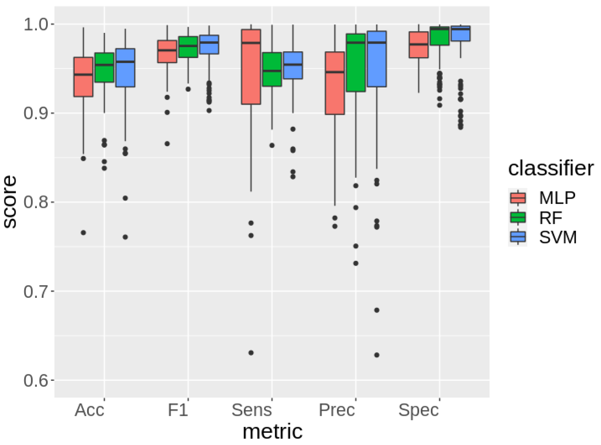
To compare machine learning algorithms with the state-of-the-art cloud detection techniques, we trained RF, SVM and MLP classifiers on the dataset ${\mathcal{D}}_1$ and assessed their robustness. An overview is presented in Figure 2.

SVM achieved the highest cross-validation performance in terms of all proposed metrics except sensitivity, in the latter case, MLP obtained the best result. The numeric values are reported to ease comparison in

Table 3. The median and $95\%$ confidence intervals for all adopted metrics are reported to compare different learning methods. In bold, we reported the higher values for each metric.

Metric (%)	$\mathit{A}\mathit{c}\mathit{c}$	$\mathit{F}1$	$\mathit{S}\mathit{e}\mathit{n}\mathit{s}$	$\mathit{P}\mathit{r}\mathit{e}\mathit{c}$	$\mathit{S}\mathit{p}\mathit{e}\mathit{c}$
SVM	97.9 (91.4, 99.6)	95.8 (85.5, 99.1)	95.4 (85.8, 99.8)	97.9 (77.2, 99.9)	99.4 (88.7, 99.9)
RF	97.5 (93.5, 99.3)	95.4 (86.4, 98.8)	94.7 (88.7, 99.7)	97.9 (80.6, 99.9)	99.4 (92.7, 100.0)
MLP	97.0 (91.9, 99.7)	94.3 (85.5, 99.4)	97.9 (78.2, 100.0)	94.6 (79.7, 99.9)	97.7 (93.9, 99.9)

.

We assessed the statistical difference of cross-validation distributions by means of a Mann–Whitney U test [48], and found that MLP performs significantly better ($5\%$) in terms of sensitivity than RF and SVM. Both SVM and RF perform significantly better ($5\%$) than MLP in terms of precision and specificity. SVM obtains the best better performance in terms of accuracy and $F1$. Moreover, we assessed the statistical difference of the variances for the performance distributions by means of a Levene Test [49]. The only significant differences we found were for the accuracy distribution of RF and the sensitivity distribution of MLP. In conclusion, RF would seem a slightly more robust segmentation method while SVM is more accurate; accordingly, for the following investigations we considered only SVM.

6.2. How Sample Size and Heterogeneity Affect Performance

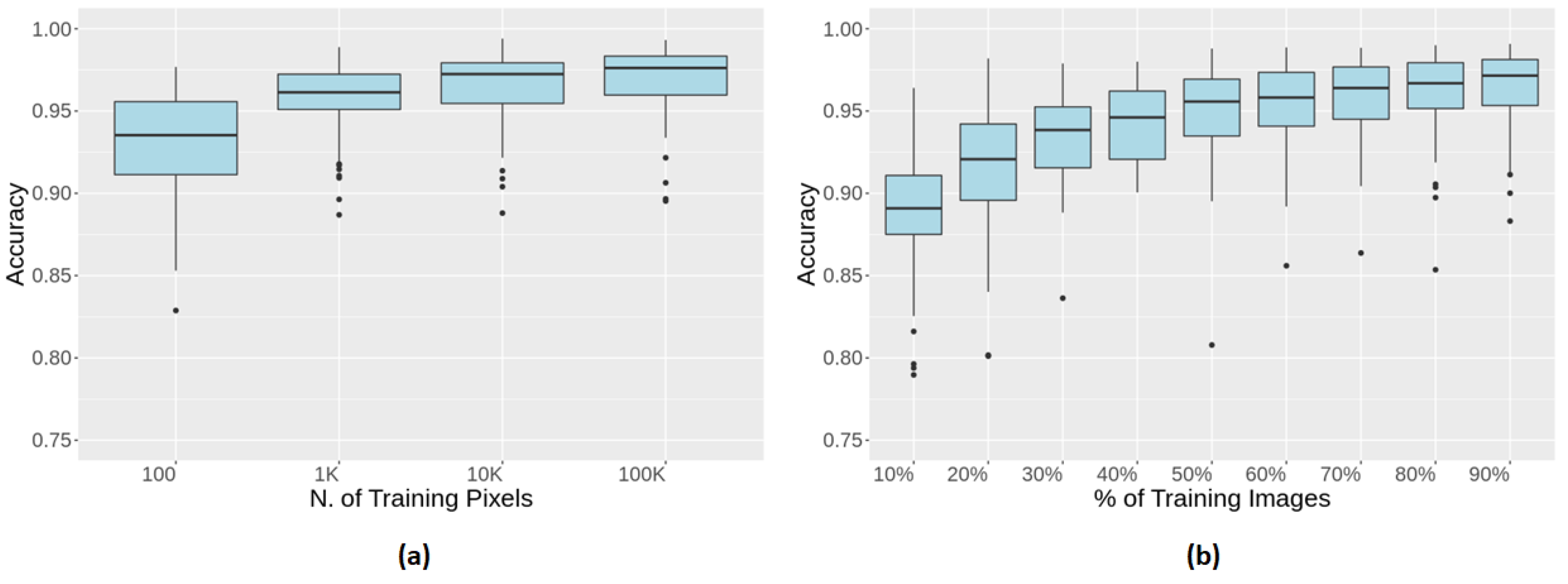
Firstly, we evaluated how training set size affected classification performance. The aim of this analysis was twofold: on the one hand, understanding whether or not it is possible to use a reduced training set size to accurately distinguish clouds form clear sky pixels; on the other hand, reducing the computational burden of learning processes. Then, we investigated how the availability of heterogeneous data affects the learning process. Using a fixed number of training examples, we sampled them from a varying number of images. The SVM results are presented in Figure 3, a similar behaviour was also observed for RF and MLP.

Left panel (a) shows how SVM performance reaches a plateau after ${10}^4$ training pixels are provided for learning. As ${10}^4$ pixels is a sufficient number of training examples to reach accurate classification, the following analyses are performed using this value. Right panel (b) shows how the number of different images affect the classification performance. In this way we evaluated the heterogeneity of ${\mathcal{D}}_1$ images. We varied the number of images used for training from $10\%$ to $90\%$ of the whole training set. Once reached $80\%$ of training images, the mean and the variance of SVM accuracy are statistically indistinguishable. For the mean, we used the Mann–Whitney U test, and for variance, a Levene Test [49].

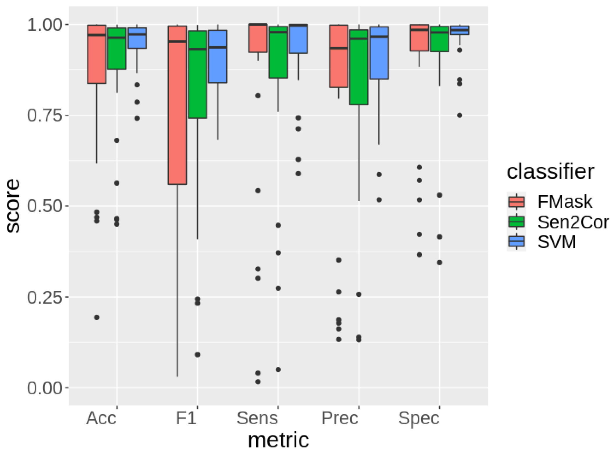
6.3. Segmentation Reliability on the Independent Test Set ${\mathcal{D}}_2$

We evaluated the reliability of SVM segmentation on an independent test set ${\mathcal{D}}_2$, which is homogeneous with ${\mathcal{D}}_1$. Furthermore, we compared our results with state-of-the-art threshold-based methods: Sen2Cor and FMask. It was not possible to evaluate MAJA on ${\mathcal{D}}_2$ as it requires a temporal series of images that for the present case were not available. Specifically, we trained SVM on ${\mathcal{D}}_1$ pixels and we evaluated its segmentation performance on ${\mathcal{D}}_2$. Results are shown in Figure 4.

SVM achieved a similar performance to the one obtained on ${\mathcal{D}}_1$, thus confirming the robustness of its segmentations. A complete overview of the comparison is presented in

Table 4. The median and $95\%$ confidence intervals for all adopted metrics are reported for all the compared methods. MAJA was excluded from this comparison as the longitudinal series of images needed for its training are not available. Best results are in bold.

Metric (%)	$\mathit{A}\mathit{c}\mathit{c}$	$\mathit{F}1$	$\mathit{S}\mathit{e}\mathit{n}\mathit{s}$	$\mathit{P}\mathit{r}\mathit{e}\mathit{c}$	$\mathit{S}\mathit{p}\mathit{e}\mathit{c}$
SVM	97.7 (78.4, 100.0)	93.6 (71.6, 100.0)	99.7 (61.8, 100.0)	96.6 (56.5, 100.0)	98.4 (83.2, 100.0)
Sen2Cor	96.4 (43.9, 100.0)	93.2 (19.4, 99.6)	97.8 (21.1, 100.0)	96.1 (13.7, 100.0)	97.8 (33.8, 100.0)
FMask	98.2 (24.9, 100.0)	95.3 (5.6, 100.0)	99.9 (3.1, 100.0)	93.5 (15.4, 100.0)	98.6 (35.8, 100.0)

.

SVM segmentations significantly ($5\%$) resulted in the best ones in terms of precision and specificity according to a paired Wilcoxon test [50]. For what concerns accuracy, $F1$ and sensitivity FMask performed slightly better than other methods. However, these differences were not statistically significant. Finally, FMask and Sen2Cor performance distributions resulted as less sharp than the SVM one ($5\%$ significance), according to the Levene Test.

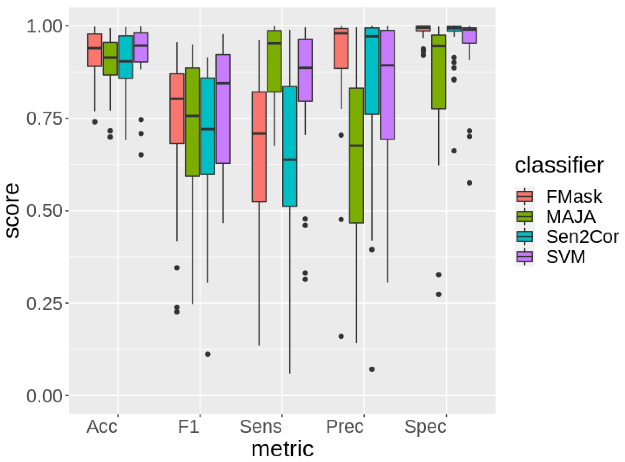
6.4. Generalization Power on ${\mathcal{D}}_3$

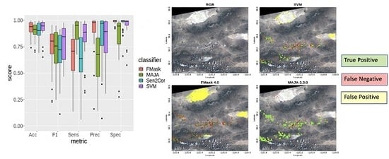
Another independent test set ${\mathcal{D}}_3$ was used to evaluate the generalization power of SVM on a set inhomogeneous with the training one. In order to accomplish such task, we trained SVM on pixels from ${\mathcal{D}}_1$ and ${\mathcal{D}}_2$ and evaluated its performance on ${\mathcal{D}}_3$. Figure 5 shows a comparison of the distribution of the classification metrics computed over the 29 scenes of the ${\mathcal{D}}_3$ dataset.

A comprehensive overview of all performance metrics is reported in

Table 5. The comparison of segmentation performance on the ${\mathcal{D}}_3$ dataset according to different metrics. In bold, we reported the higher values for each validation metric.

Metric (%)	$\mathit{A}\mathit{c}\mathit{c}$	$\mathit{F}1$	$\mathit{S}\mathit{e}\mathit{n}\mathit{s}$	$\mathit{P}\mathit{r}\mathit{e}\mathit{c}$	$\mathit{S}\mathit{p}\mathit{e}\mathit{c}$
SVM	94.7 (69.1, 99.6)	84.5 (47.5, 96.2)	88.2 (32.6, 99.3)	89.3 (33.2, 99.8)	99.0 (66.3, 100.0)
FMask	94.0 (76.1, 99.8)	80.3 (23.5, 93.8)	70.9 (18.7, 96.0)	98.0 (38.2, 100.0)	99.5 (92.8, 100.0)
MAJA	91.5 (71.1, 98.3)	75.7 (30.4, 94.7)	95.3(70.4, 99.8)	67.6 (18.2, 98.8)	94.6 (31.1, 99.6)
Sen2Cor	90.4 (71.3, 99.5)	72.1 (11.2, 91.3)	63.8 (14.4, 98.7)	97.2 (29.8, 100.0)	99.4 (79.6, 100.0)

.

SVM significantly ($5\%$) resulted in the best performing method in terms of accuracy and $F1$ according to a paired Wilcoxon test. Conversely, FMask is significantly more accurate than Sen2Cor while no significant difference in terms of accuracy can be assessed between MAJA and FMask. Furthermore, SVM is the most balanced segmentation strategy as it can be observed in terms of the $95\%$ confidence intervals; this difference is statistically significant according to the Levene test. MAJA is significantly ($5\%$) the best segmentation method in terms of sensitivity, followed by SVM. FMask is the second method in terms of $F1$, it has high specificity but a significant lower sensitivity compared to MAJA and SVM. 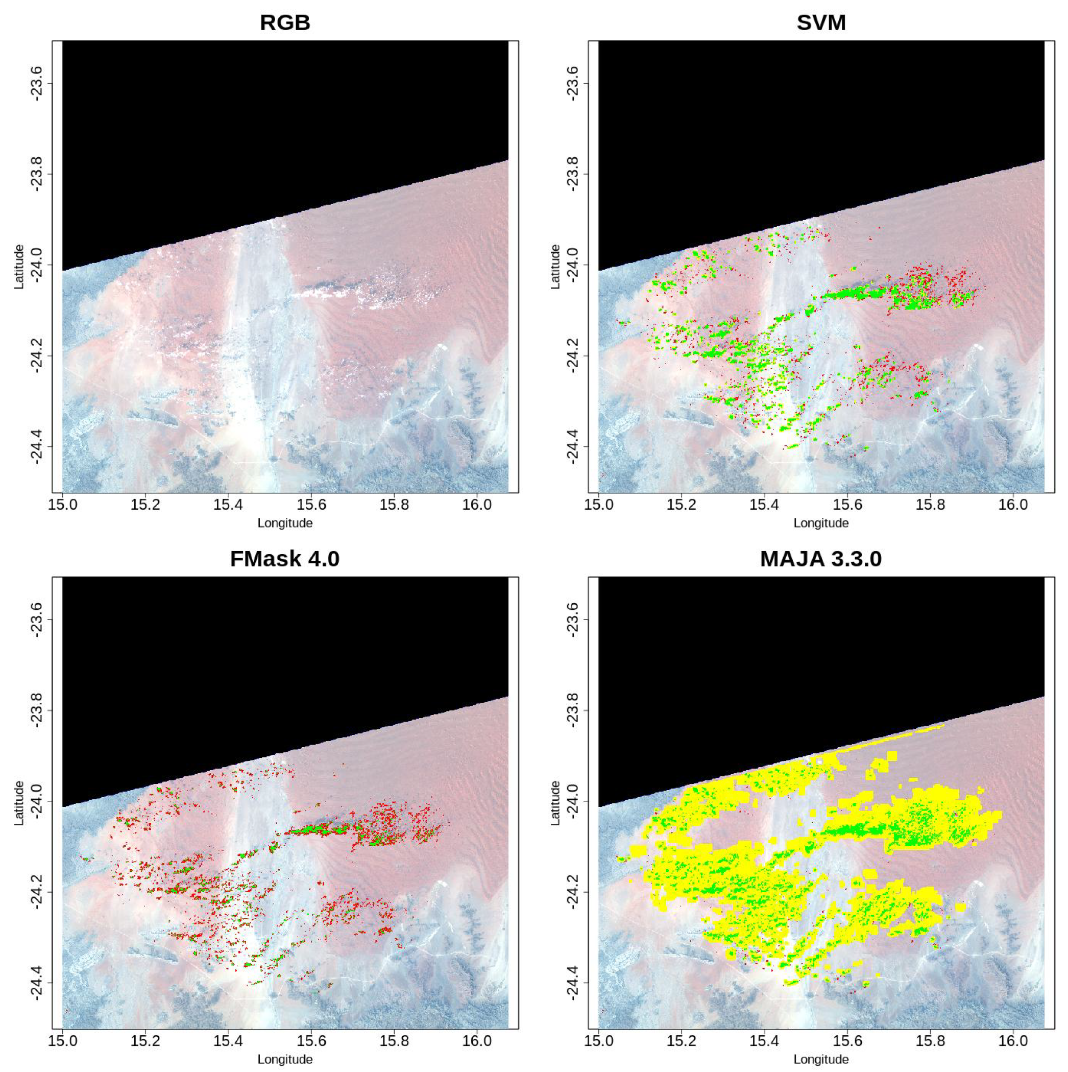Finally, Sen2Cor is the least accurate in terms of accuracy and $F1$, but with remarkable precision and specificity, where it scored as the second. A visual assessment of these results is shown in Figure 6.

SVM provides a balanced segmentation between false negative and false positive errors. FMask and MAJA segmentations tend to prefer false negatives and false positives, respectively; Sen2Cor was not considered here as its segmentations tend to be similar to those obtained by FMask.

7. Discussion

This study proposed a comparison of machine learning and threshold-based techniques for cloud detection and segmentation in Sentinel-2 L1C images. In order to enable an unbiased performance comparison, we first built and validated supervised learning models, namely SVM, RF and MLP, with a cross-validation procedure on a training set ${\mathcal{D}}_1$. Machine learning strategies achieve extremely accurate performances, despite the exiguous number of features used; in this work we used only the 13 spectral band intensities and the GTOPO30 digital elevation feature. Although all machine learning strategies were accurate, SVM performed slightly better than the other classifiers in almost all metrics; MLP was the most sensitive method and RF the one with less variance.

For what concerns MLP, it is worth noting that we explored several deep neural network configurations, but a shallow one resulted in the best performing. This is particularly striking compared with the RF performance; it is reasonable to conclude that when dealing with pixel-based approaches, deep learning cannot exploit their full potential as they certainly do in other situations and with other approaches, for example when considering Convolutional Neural Networks (CNN) [51,52]. To this purpose, it should also be noted that CNN algorithms cannot be suitably applied to whatever data format; in particular, in this study we used images with labelled polygons of varying size and shape, a typical situation in remote sensing imagery, thus it is not possible to adopt ready-to-use CNN solutions, and specific solutions and customizations would be required. In this sense, standard learning algorithms, which simply require labelled pixels as the base of knowledge, represent an efficient, user-friendly and therefore still valuable solution for several engineering purposes [53,54].

Furthermore, we evaluated how, despite the increasing size of the training set for remote sensing applications, machine learning strategies remain an efficient tool for segmentation as they require relatively small-size training sets. According to our experiments, ${10}^4$ pixels collected from ∼20 scenes provide a sufficiently accurate classification. This analysis confirmed the robustness of machine learning strategies, in fact for all the classifiers showed a common behaviour.

Typically, a Sentinel-2 acquisition covers a swath of 298 km roughly corresponding to three distinct but adjacent images. Of course, these images are strongly correlated, thus to avoid results biased by spatial correlations we always kept adjacent tiles within the same cross-validation fold. Previous works in remote sensing and other fields have outlined the danger of double dipping in machine learning [47,55], especially for generalization purposes. As demonstrated elsewhere [21,56], generalization remains the most difficult challenge to tackle for learning algorithms. Accordingly, we evaluated the performance of our best machine learning strategy on an independent test set and compared it with model-based segmentations.

A first evaluation was performed using the independent test set ${\mathcal{D}}_2$, which was labelled by the same experts of ${\mathcal{D}}_1$; we observed that SVM substantially reproduced the performances observed on ${\mathcal{D}}_1$. These findings remark that when training and validation data are homogeneous (e.g., same geographical regions and same segmentation protocols) learning strategies like SVM can provide reliable segmentations. SVM achieved comparable performance with the state-of-the-art methodologies Sen2Cor and FMask. Notably, SVM segmentations were significantly more accurate in terms of precision and specificity. Furthermore, we observed that SVM segmentations were statistically less prone to drastic failures, thus yielding performance distributions affected by less variability, an effect demonstrated by a Levene test. This result can represent a particularly interesting feature, as it suggests that in some cases learning-based approaches are more robust.

A second evaluation was performed using the test set ${\mathcal{D}}_3$, which for its characteristics could be considered not homogeneous with ${\mathcal{D}}_1$. SVM remained the best performing method in terms of accuracy ($94.7\%$) and $F1$ ($84.5\%$). Although homogeneity of training and test data is a primary issue for machine learning accuracy [57,58], the only statistically significant drop in performance we observed were ∼4% in accuracy and ∼10% in $F1$. 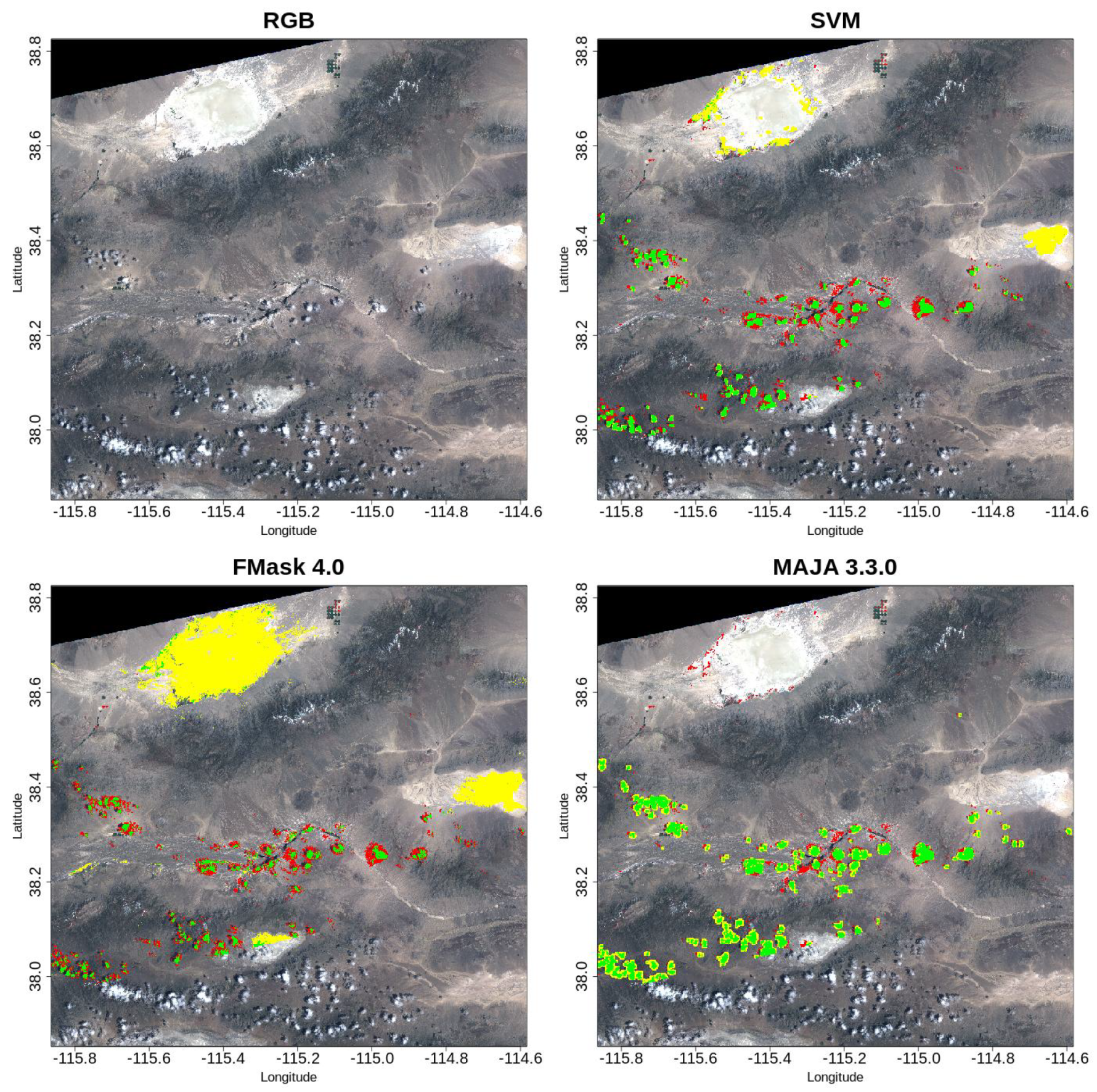MAJA was able to provide segmentations more accurate than SVM and other methods in a few cases. An example is shown in Figure 7.

As can be seen, MAJA gets the most accurate cloud classification on a barren area. In these regions, characterized by high reflectance, the multi-temporal base of knowledge allows a correct classification of bright surfaces, which otherwise could be classified as clouds [10,11,59].

In general, MAJA resulted in the most sensitive ($95.3\%$) method and FMask resulted in the most precise ($98.0\%$) and specific ($99.5\%$); however, it is worth noting that according to specificity the difference with Sen2Cor is negligible ($99.4\%$). These findings should be taken into consideration as the main purpose of cloud detection is avoiding false positives, especially for change detection or land cover applications [23,25,60,61]. Nevertheless, learning strategies and specifically SVM seem to provide more balanced classifications, which can achieve better results, especially in terms of metrics evaluating the overall performance as accuracy and $F1$.

8. Conclusions

In this work, we developed a pixel-based classification procedure based on machine learning techniques for cloud detection in Sentinel-2 data. We evaluated different supervised models: RF, SVM and MLP. Our analyses demonstrated that, among learning models, SVM is the best option. In addition, we compared SVM with state-of-the-art model-based methodologies such as MAJA, FMask and Sen2Cor. We evaluated how data homogeneity affects the segmentations using two independent test sets, the first one collected and segmented with the same procedures of our training set and the second characterized by a deep heterogeneity. In both cases, SVM was the best performing method in terms of accuracy and $F1$. Nonetheless, all different strategies have strengths and weaknesses: MAJA resulted in the most sensitive method, FMask and Sen2Cor were the most precise. The access to homogeneous data remains a key issue, in fact when using not homogeneous data, we observed a slight but significant drop in performance. The comparison with model-based segmentation suggests that learning methods can improve their performance when trained on temporal series, an aspect that deserves future investigations. Our findings demonstrate the accuracy of standard machine learning methods, especially SVM as a valid alternative to state-of-the-art segmentation strategies. As far as we know, this work presents the most extensive comparison between machine learning and model-based segmentations. Furthermore, other studies comparing different segmentation strategies focused on small data usually covering homogeneous environments. As far as we know, this is the first work considering learning procedures and comparing them with model-based approaches for world-scale analyses, whilst regional scale analyses are usually preferred. Future studies should consider the design and customization of CNN architectures for this data; another interesting aspect to consider is the investigation of eventual differences in segmentation performance between Sentinel and Landsat data.

References

- Roy, D.P.; Ju, J.; Kline, K.; Scaramuzza, P.L.; Kovalskyy, V.; Hansen, M.; Loveland, T.R.; Vermote, E.; Zhang, C. Web-enabled Landsat Data (WELD): Landsat ETM+ composited mosaics of the conterminous United States. Remote Sens. Environ. 2010, 114, 35–49. [Google Scholar] [CrossRef]
- Louis, J.; Debaecker, V.; Pflug, B.; Main-Knorn, M.; Bieniarz, J.; Mueller-Wilm, U.; Cadau, E.; Gascon, F. Sentinel-2 sen2cor: L2a processor for users. In Proceedings of the Living Planet Symposium, Prague, Czech Republic, 9–13 May 2016; pp. 9–13. [Google Scholar]
- Vermote, E.F.; El Saleous, N.Z.; Justice, C.O. Atmospheric correction of MODIS data in the visible to middle infrared: First results. Remote Sens. Environ. 2002, 83, 97–111. [Google Scholar] [CrossRef]
- Huete, A.; Didan, K.; Miura, T.; Rodriguez, E.P.; Gao, X.; Ferreira, L.G. Overview of the radiometric and biophysical performance of the MODIS vegetation indices. Remote Sens. Environ. 2002, 83, 195–213. [Google Scholar] [CrossRef]
- Zhang, Y.; Guindon, B.; Cihlar, J. An image transform to characterize and compensate for spatial variations in thin cloud contamination of Landsat images. Remote Sens. Environ. 2002, 82, 173–187. [Google Scholar] [CrossRef]
- Zhu, Z.; Woodcock, C.E. Automated cloud, cloud shadow, and snow detection in multitemporal Landsat data: An algorithm designed specifically for monitoring land cover change. Remote Sens. Environ. 2014, 152, 217–234. [Google Scholar] [CrossRef]
- Lu, D.; Weng, Q. A survey of image classification methods and techniques for improving classification performance. Int. J. Remote Sens. 2007, 28, 823–870. [Google Scholar] [CrossRef]
- Irish, R.R.; Barker, J.L.; Goward, S.N.; Arvidson, T. Characterization of the Landsat-7 ETM+ automated cloud-cover assessment (ACCA) algorithm. Photogramm. Eng. Remote Sens. 2006, 72, 1179–1188. [Google Scholar] [CrossRef]
- Zhu, Z.; Woodcock, C.E. Object-based cloud and cloud shadow detection in Landsat imagery. Remote Sens. Environ. 2012, 118, 83–94. [Google Scholar] [CrossRef]
- Bley, S.; Deneke, H. A threshold-based cloud mask for the high-resolution visible channel of Meteosat Second Generation SEVIRI. Atmos. Meas. Tech. 2013, 6, 2713–2723. [Google Scholar] [CrossRef]
- Coluzzi, R.; Imbrenda, V.; Lanfredi, M.; Simoniello, T. A first assessment of the Sentinel-2 Level 1-C cloud mask product to support informed surface analyses. Remote Sens. Environ. 2018, 217, 426–443. [Google Scholar] [CrossRef]
- Hagolle, O.; Huc, M.; Pascual, D.V.; Dedieu, G. A multi-temporal method for cloud detection, applied to FORMOSAT-2, VENμS, LANDSAT and SENTINEL-2 images. Remote Sens. Environ. 2010, 114, 1747–1755. [Google Scholar] [CrossRef]
- Mateo-García, G.; Gómez-Chova, L.; Amorós-López, J.; Muñoz-Marí, J.; Camps-Valls, G. Multitemporal cloud masking in the Google Earth Engine. Remote Sens. 2018, 10, 1079. [Google Scholar] [CrossRef]
- Niemeyer, J.; Rottensteiner, F.; Soergel, U. Contextual classification of lidar data and building object detection in urban areas. ISPRS J. Photogramm. Remote Sens. 2014, 87, 152–165. [Google Scholar] [CrossRef]
- Shao, Z.; Deng, J.; Wang, L.; Fan, Y.; Sumari, N.; Cheng, Q. Fuzzy autoencode based cloud detection for remote sensing imagery. Remote Sens. 2017, 9, 311. [Google Scholar] [CrossRef]
- Shendryk, Y.; Rist, Y.; Ticehurst, C.; Thorburn, P. Deep learning for multi-modal classification of cloud, shadow and land cover scenes in PlanetScope and Sentinel-2 imagery. ISPRS J. Photogramm. Remote Sens. 2019, 157, 124–136. [Google Scholar] [CrossRef]
- Zi, Y.; Xie, F.; Jiang, Z. A Cloud Detection Method for Landsat 8 Images Based on PCANet. Remote Sens. 2018, 10, 877. [Google Scholar] [CrossRef]
- Mateo-García, G.; Laparra, V.; López-Puigdollers, D.; Gómez-Chova, L. Transferring deep learning models for cloud detection between Landsat-8 and Proba-V. ISPRS J. Photogramm. Remote Sens. 2020, 160, 1–17. [Google Scholar] [CrossRef]
- Platnick, S.; King, M.D.; Ackerman, S.A.; Menzel, W.P.; Baum, B.A.; Riédi, J.C.; Frey, R.A. The MODIS cloud products: Algorithms and examples from Terra. IEEE Trans. Geosci. Remote Sens. 2003, 41, 459–473. [Google Scholar] [CrossRef]
- Sanchez, A.H.; Picoli, M.C.A.; Camara, G.; Andrade, P.R.; Chaves, M.E.D.; Lechler, S.; Soares, A.R.; Marujo, R.F.B.; Simões, R.E.O.; Ferreira, K.R.; et al. Comparison of Cloud Cover Detection Algorithms on Sentinel-2 Images of the Amazon Tropical Forest. Remote Sens. 2020, 12, 1284. [Google Scholar] [CrossRef]
- Amoroso, N.; Diacono, D.; Fanizzi, A.; La Rocca, M.; Monaco, A.; Lombardi, A.; Guaragnella, C.; Bellotti, R.; Tangaro, S.; Initiative, A.D.N.; et al. Deep learning reveals Alzheimer’s disease onset in MCI subjects: Results from an international challenge. J. Neurosci. Methods 2018, 302, 3–9. [Google Scholar] [CrossRef]
- Choobdar, S.; Ahsen, M.E.; Crawford, J.; Tomasoni, M.; Fang, T.; Lamparter, D.; Lin, J.; Hescott, B.; Hu, X.; Mercer, J.; et al. Assessment of network module identification across complex diseases. Nat. Methods 2019, 16, 843–852. [Google Scholar] [CrossRef] [PubMed]
- Hollstein, A.; Segl, K.; Guanter, L.; Brell, M.; Enesco, M. Ready-to-use methods for the detection of clouds, cirrus, snow, shadow, water and clear sky pixels in Sentinel-2 MSI images. Remote Sens. 2016, 8, 666. [Google Scholar] [CrossRef]
- Available Data. Available online: https://github.com/hollstein/cB4S2 (accessed on 24 August 2019).
- Baetens, L.; Desjardins, C.; Hagolle, O. Validation of Copernicus Sentinel-2 Cloud Masks Obtained from MAJA, Sen2Cor, and FMask Processors Using Reference Cloud Masks Generated with a Supervised Active Learning Procedure. Remote Sens. 2019, 11, 433. [Google Scholar] [CrossRef]
- Baetens, L.; Hagolle, O. Sentinel-2 reference cloud masks generated by an active learning method. Zenodo 2018. [Google Scholar] [CrossRef]
- Gao, B.C.; Goetz, A.F.H.; Wiscombe, W.J. Cirrus cloud detection from Airborne Imaging Spectrometer data using the 1.38 μm water vapor band. Geophys. Res. Lett. 1993, 20. [Google Scholar] [CrossRef]
- USGS 30 ARC-Second Global Elevation Data, GTOPO30; NCAR Computational and Information Systems Laboratory: Boulder, CO, USA, 1997.
- Dozier, J. Spectral signature of alpine snow cover from the Landsat Thematic Mapper. Remote Sens. Environ. 1989, 28, 9–22. [Google Scholar] [CrossRef]
- Richter, R.; Louis, J.; Müller-Wilm, U. Sentinel-2 msi–level 2a products algorithm theoretical basis document. Eur. Space Agency (Spec. Publ.) ESA SP 2012, 49, 1–72. [Google Scholar]
- Zhu, Z.; Wang, S.; Woodcock, C.E. Improvement and expansion of the Fmask algorithm: Cloud, cloud shadow, and snow detection for Landsats 4–7, 8, and Sentinel 2 images. Remote Sens. Environ. 2015, 159, 269–277. [Google Scholar] [CrossRef]
- Frantz, D.; Haß, E.; Uhl, A.; Stoffels, J.; Hill, J. Improvement of the Fmask algorithm for Sentinel-2 images: Separating clouds from bright surfaces based on parallax effects. Remote Sens. Environ. 2018, 215, 471–481. [Google Scholar] [CrossRef]
- Qiu, S.; Zhu, Z.; He, B. Fmask 4.0: Improved cloud and cloud shadow detection in Landsats 4–8 and Sentinel-2 imagery. Remote Sens. Environ. 2019, 231, 111205. [Google Scholar] [CrossRef]
- Lyapustin, A.; Wang, Y.; Frey, R. An automatic cloud mask algorithm based on time series of MODIS measurements. J. Geophys. Res. Atmos. 2008, 113. Available online: https://agupubs.onlinelibrary.wiley.com/doi/pdf/10.1029/2007JD009641 (accessed on 21 May 2020). [CrossRef]
- Breiman, L. Random forests. Mach. Learn. 2001, 45, 5–32. [Google Scholar] [CrossRef]
- Belgiu, M.; Drăguţ, L. Random forest in remote sensing: A review of applications and future directions. ISPRS J. Photogramm. Remote Sens. 2016, 114, 24–31. [Google Scholar] [CrossRef]
- Gislason, P.O.; Benediktsson, J.A.; Sveinsson, J.R. Random forests for land cover classification. Pattern Recognit. Lett. 2006, 27, 294–300. [Google Scholar] [CrossRef]
- Liaw, A.; Wiener, M. Classification and Regression by randomForest. R News 2002, 2, 18–22. [Google Scholar]
- Cortes, C.; Vapnik, V. Support-vector networks. Mach. Learn. 1995, 20, 273–297. [Google Scholar] [CrossRef]
- Mountrakis, G.; Im, J.; Ogole, C. Support vector machines in remote sensing: A review. ISPRS J. Photogramm. Remote Sens. 2011, 66, 247–259. [Google Scholar] [CrossRef]
- Meyer, D.; Dimitriadou, E.; Hornik, K.; Weingessel, A.; Leisch, F. e1071: Misc Functions of the Department of Statistics, Probability Theory Group (Formerly: E1071), TU Wien, R package version 1.7-3; R Foundation for Statistical Computing: Vienna, Austria, 2019. [Google Scholar]
- Le Cun, Y. Learning process in an asymmetric threshold network. In Disordered Systems and Biological Organization; Springer: Berlin/Heidelberg, Germany, 1986; pp. 233–240. [Google Scholar]
- Hecht-Nielsen, R. Theory of the backpropagation neural network. In Neural Networks for Perception; Elsevier: Amsterdam, The Netherlands, 1992; pp. 65–93. [Google Scholar]
- Rumelhart, D.E.; Hinton, G.E.; Williams, R.J. Learning representations by back-propagating errors. Nature 1986, 323, 533–536. [Google Scholar] [CrossRef]
- LeDell, E.; Gill, N.; Aiello, S.; Fu, A.; Candel, A.; Click, C.; Kraljevic, T.; Nykodym, T.; Aboyoun, P.; Kurka, M.; et al. h2o: R Interface for the ’H2O’ Scalable Machine Learning Platform, R package version 3.28.0.4; R Foundation for Statistical Computing: Vienna, Austria, 2020. [Google Scholar]
- Bergstra, J.; Bengio, Y. Random search for hyper-parameter optimization. J. Mach. Learn. Res. 2012, 13, 281–305. [Google Scholar]
- Maggipinto, T.; Bellotti, R.; Amoroso, N.; Diacono, D.; Donvito, G.; Lella, E.; Monaco, A.; Scelsi, M.A.; Tangaro, S.; Initiative, A.D.N.; et al. DTI measurements for Alzheimer’s classification. Phys. Med. Biol. 2017, 62, 2361. [Google Scholar] [CrossRef]
- Mann, H.B.; Whitney, D.R. On a Test of Whether one of Two Random Variables is Stochastically Larger than the Other. Ann. Math. Stat. 1947, 18, 50–60. [Google Scholar] [CrossRef]
- Brown, M.B.; Forsythe, A.B. Robust Tests for the Equality of Variances. J. Am. Stat. Assoc. 1974, 69, 364–367. Available online: https://www.tandfonline.com/doi/pdf/10.1080/01621459.1974.10482955 (accessed on 21 May 2020). [CrossRef]
- Wilcoxon, F. Individual Comparisons by Ranking Methods. Biom. Bull. 1945, 1, 80–83. [Google Scholar] [CrossRef]
- Nogueira, K.; Penatti, O.A.; Dos Santos, J.A. Towards better exploiting convolutional neural networks for remote sensing scene classification. Pattern Recognit. 2017, 61, 539–556. [Google Scholar] [CrossRef]
- Ball, J.E.; Anderson, D.T.; Chan, C.S. Comprehensive survey of deep learning in remote sensing: Theories, tools, and challenges for the community. J. Appl. Remote Sens. 2017, 11, 042609. [Google Scholar] [CrossRef]
- Yu, Y.; Dackermann, U.; Li, J.; Niederleithinger, E. Wavelet packet energy–based damage identification of wood utility poles using support vector machine multi-classifier and evidence theory. Struct. Health Monit. 2019, 18, 123–142. [Google Scholar] [CrossRef]
- Su, Z.; Ye, L. Quantitative damage prediction for composite laminates based on wave propagation and artificial neural networks. Struct. Health Monit. 2005, 4, 57–66. [Google Scholar] [CrossRef]
- Kriegeskorte, N.; Simmons, W.K.; Bellgowan, P.S.; Baker, C.I. Circular analysis in systems neuroscience: The dangers of double dipping. Nat. Neurosci. 2009, 12, 535. [Google Scholar] [CrossRef]
- Cohn, D.; Atlas, L.; Ladner, R. Improving generalization with active learning. Mach. Learn. 1994, 15, 201–221. [Google Scholar] [CrossRef]
- L’heureux, A.; Grolinger, K.; Elyamany, H.F.; Capretz, M.A. Machine learning with big data: Challenges and approaches. IEEE Access 2017, 5, 7776–7797. [Google Scholar] [CrossRef]
- Claverie, M.; Ju, J.; Masek, J.G.; Dungan, J.L.; Vermote, E.F.; Roger, J.C.; Skakun, S.V.; Justice, C. The Harmonized Landsat and Sentinel-2 surface reflectance data set. Remote Sens. Environ. 2018, 219, 145–161. [Google Scholar] [CrossRef]
- Li, Z.; Shen, H.; Cheng, Q.; Liu, Y.; You, S.; He, Z. Deep learning based cloud detection for medium and high resolution remote sensing images of different sensors. ISPRS J. Photogramm. Remote Sens. 2019, 150, 197–212. [Google Scholar] [CrossRef]
- Foga, S.; Scaramuzza, P.L.; Guo, S.; Zhu, Z.; Dilley, R.D.; Beckmann, T.; Schmidt, G.L.; Dwyer, J.L.; Hughes, M.J.; Laue, B. Cloud detection algorithm comparison and validation for operational Landsat data products. Remote Sens. Environ. 2017, 194, 379–390. [Google Scholar] [CrossRef]
- Yang, X.; Jia, Z.; Yang, J.; Kasabov, N. Change Detection of Optical Remote Sensing Image Disturbed by Thin Cloud Using Wavelet Coefficient Substitution Algorithm. Sensors 2019, 19, 1972. [Google Scholar] [CrossRef] [PubMed]
Figure 1.
Global distribution of Sentinel-2 scenes included in the data sets used in this work.
Figure 2.
Performance estimation in terms of each metric, on cross validation, of Multilayer Perceptrons (MLP), Random Forest (RF) and Support Vector Machines (SVM) trained with randomly sampled pixel for cloud detection task.
Figure 3.
(a) Accuracy of the SVM classifier increases with the number of training examples: after pixels are provided no significant improvement is registered. (b) The effect of heterogeneity on performance: despite the equal number of training examples (), only after of images are used, the performance reaches stable values.
Figure 4.
Performance comparison of FMask, Sen2Cor and SVM.
Figure 5.
Performance estimation, on the independent test set, of FMask, MAJA, Sen2Cor and SVM in terms of each classification metric. The classification metrics are evaluated over the 29 scenes of .
Figure 6.
The top left image shows the RGB image from Gobabeb, Namibia, on 9 September 2017. The three other images show the comparison of each procedure (as default) to the reference mask (top-right, SVM, bottom-left, FMask, and bottom-right, MAJA). Green colour corresponds to true positive, red colour to false negative, and yellow to false positive.
Figure 7.
The top left image shows the RGB image from Railroad Valley, Nevada on 1 May 2017. The three other images show the comparison of each procedure (as default) to the reference mask (top-right, SVM, bottom-left, FMask, and bottom-right, MAJA). Green colour corresponds to true positive, red colour to false negative, and yellow to false positive.