Article

IrrMapper: A Machine Learning Approach for High Resolution Mapping of Irrigated Agriculture Across the Western U.S.

1
Montana Climate Office, W.A. Franke College of Forestry and Conservation, University of Montana, Missoula, MT 59812, USA
2
Department of Geosciences, University of Montana, Missoula, MT 59812, USA
3
Department of Ecosystem and Conservation Sciences, W.A. Franke College of Forestry and Conservation, University of Montana, Missoula, MT 59812, USA
4
School of Natural Sciences, California State University Monterey Bay, Seaside, CA 93955, USA
5
Cooperative for Research in Earth Science and Technology, NASA Ames Research Center, Moffett Field, CA 94035, USA
6
Numerical Terradynamic Simulation Group, University of Montana, Missoula, MT 59812, USA
7
Division of Hydrologic Sciences, Western Regional Climate Center, Desert Research Institute, Reno, NV 89512, USA
*
Author to whom correspondence should be addressed.
Remote Sens. 2020, 12(14), 2328; https://doi.org/10.3390/rs12142328
Submission received: 15 May 2020 / Revised: 9 July 2020 / Accepted: 14 July 2020 / Published: 20 July 2020

Abstract

:
High frequency and spatially explicit irrigated land maps are important for understanding the patterns and impacts of consumptive water use by agriculture. We built annual, 30 m resolution irrigation maps using Google Earth Engine for the years 1986–2018 for 11 western states within the conterminous U.S. Our map classifies lands into four classes: irrigated agriculture, dryland agriculture, uncultivated land, and wetlands. We built an extensive geospatial database of land cover from each class, including over 50,000 human-verified irrigated fields, 38,000 dryland fields, and over 500,000 km 2 of uncultivated lands. We used 60,000 point samples from 28 years to extract Landsat satellite imagery, as well as climate, meteorology, and terrain data to train a Random Forest classifier. Using a spatially independent validation dataset of 40,000 points, we found our classifier has an overall binary classification (irrigated vs. unirrigated) accuracy of 97.8%, and a four-class overall accuracy of 90.8%. We compared our results to Census of Agriculture irrigation estimates over the seven years of available data and found good overall agreement between the 2832 county-level estimates (r 2 = 0.90), and high agreement when estimates are aggregated to the state level (r 2 = 0.94). We analyzed trends over the 33-year study period, finding an increase of 15% (15,000 km 2 ) in irrigated area in our study region. We found notable decreases in irrigated area in developing urban areas and in the southern Central Valley of California and increases in the plains of eastern Colorado, the Columbia River Basin, the Snake River Plain, and northern California.

1. Introduction

In the Western U.S., over 80% of extracted freshwater is used for irrigation (i.e., artificial application of water to crops by humans), 56% of which is consumed by crops (i.e., lost to the atmosphere) [1]. In this region, only one third of total cropland area is irrigated, yet irrigated farmland accounted for nearly two thirds of total commodities revenue in 2012 [2]. Irrigation is necessary to agricultural production in arid areas where precipitation is insufficient to grow food crops. Irrigation increases yields and decouples crop yields from climatic constraints [3,4], buffers against extreme weather events [5,6], and modifies temperature, humidity, and precipitation regimes at local to regional scales [7,8,9,10] and evapotranspiration (ET) globally [11]. Irrigation may also cause significant environmental impacts, including the draining or maintaining of wetlands [12,13], disrupted sedimentation [14], increased soil salinity [15], altered stream temperatures [16], changes in water table elevation [17,18], decreased stream flow [19], and changes in peak runoff rates and base flows [20,21]. Despite its economic and ecological importance, the extent and distribution of irrigation is poorly mapped in the U.S.
The most robust accounting of irrigated area in the U.S. are county-level statistics included in the Census of Agriculture, an effort undertaken since 1840 by the precursor to the U.S. Census Bureau, and currently conducted and managed by the U.S. Department of Agriculture, National Agricultural Statistics Service (NASS) [22]. NASS produces a semi-decadal estimate of per-county irrigated area based on survey responses from agricultural producers. These data lack any explicit spatial information indicating where irrigation occurs within each county. In addition, the irrigation survey is subject to potential error resulting from undercoverage, nonresponse, and misclassification of farm operations. One example of this potential error is from the 2012 census, which required an adjustment of the estimated number of operating farms of nearly 35% to correct for undercoverage [23]. Irrigated areas are self-reported and only required for farm operations meeting a revenue threshold, and therefore exclude irrigation operations on non-revenue-generating agricultural operations. The infrequency and lack of explicit spatial information of the Census of Agriculture creates a need for explicit spatial and temporal estimates of irrigated areas to improve census statistics, consumptive water use estimates, and agricultural, ecological, and water resource management.
Satellite remote sensing (SRS) is finding increasing use in approaches to identify and monitor ecological and agricultural processes at global to local scales, utilizing a variety of instruments [24,25,26]. Researchers have found utility in SRS to monitor many surface and atmospheric phenomena, including soil moisture [27], water quality [28], snow cover [29], and stream flow [30]. Advances in estimating ET using SRS methods [31,32,33,34] have enabled explicit spatial and temporal accounting of consumptive water use rates from irrigation, however lack of frequent, high-resolution maps of irrigated areas has limited the ability to accurately estimate and summarize consumptive water use volumes from irrigated areas. Volumes of consumptive water use are ultimately needed for improving natural resource management, modeling, and prediction.
SRS is well suited for efficiently identifying irrigation in space and time due to the fact that irrigated areas often have a distinct spectral signature when compared to surrounding natural vegetation or unirrigated lands, and can be identified by orbiting satellites that acquire imagery at regular and frequent intervals, and are free and open for scientific use [35,36,37]. Freely available satellite data are subject to trade-offs among overpass frequency, period of record, and spatial resolution. For example, the Moderate Resolution Imaging Spectroradiometer (MODIS) instruments on board Terra and Aqua satellites have daily, morning and afternoon overpass frequency, but the 250-m spatial resolution of the images makes identification of irrigation for individual fields difficult due to mixed pixel and field edge effects [35]. The MultiSpectral Instrument (MSI) on board Sentinel 2a and 2b satellites acquires images at 10 m spatial resolution, and has an overpass frequency of five days since the launch of Sentinel 2b in 2017. While Sentinel’s short record limits the utility for mapping irrigation history, it acquires data in comparable spectral bands to Landsat, and thus can be harmonized to map historical irrigated areas into the future [38]. Landsat Thematic Mapper (TM), Enhanced Thematic Mapper Plus (ETM+), Optical Land Imager (OLI), and Thermal Infrared Sensor (TIRS) observations provide an unmatched consistent and continuous data record of optical and thermal imagery from 1984 to present at 8–16-day frequency, and at 30-m spatial resolution—a scale well suited for observing the spatial extent and variability of individual agricultural fields and associated volumes of consumptive water use [39].
Previous SRS studies focused on mapping regional to global-scale irrigation often depend on census estimates of irrigated land area or existing land-use and land-cover datasets to parameterize irrigation models. Examples include the Global Irrigated Area Map (GIAM [40,41,42]), Landsat-based irrigation dataset (LANID [43]), and the Moderate Resolution Imaging Spectroradiometer Irrigated Agriculture Dataset for the U.S. (MIrAD-US [44,45]). These studies aim to reproduce the reported irrigated extent with added spatial detail, often using a greenness index threshold in which pixels are considered irrigated. While several studies produce annual irrigated lands data [46,47,48,49,50,51], to our knowledge, none are available for the Western U.S. A significant advance in annual, high resolution mapping of irrigated areas was recently achieved over the High Plains Aquifer (HPA) of the Central U.S. by Deines et al. [50,51]. This approach used an independently developed dataset to train a Random Forest (RF) model, a non-parametric ensemble decision tree classification and regression algorithm [52]. They mapped historical irrigated lands annually from 1984 to 2017 at 30-m resolution within a 625,000 km 2 study area with 91.4% overall accuracy. They used a novel approach to overcome imagery gaps and commission errors, and parameterized their model with neighborhood greenness indices and many ancillary datasets. Drivers of irrigated area [50] and projections of High Plains Aquifer decline [51] were also studied.
RF has been successfully implemented in many SRS-based land classification studies on mixed land types [53,54,55], and for classification of agricultural land uses [56,57,58,59,60]. RF has been shown to be a reliable and fast algorithm for remote sensing applications, suited to handling high-dimensional and colinear data, insensitive to overfitting, and explanatory of variable importance [61].
Here, we describe a Landsat-based irrigation detection RF model, IrrMapper, to map annual irrigation status at 30-m resolution. We use a similar approach and build on the previous work of Deines [50], by expanding the spatial scope and parameterizing the RF model with more extensive training, climate, land use, and other geospatial datasets. IrrMapper produces irrigation status wall-to-wall across the Western U.S., and is independent of USDA NASS irrigation statistics, allowing for an independent comparison to Census of Agriculture data as described in the following sections.

2. Data and Methods

2.1. Methodological Overview
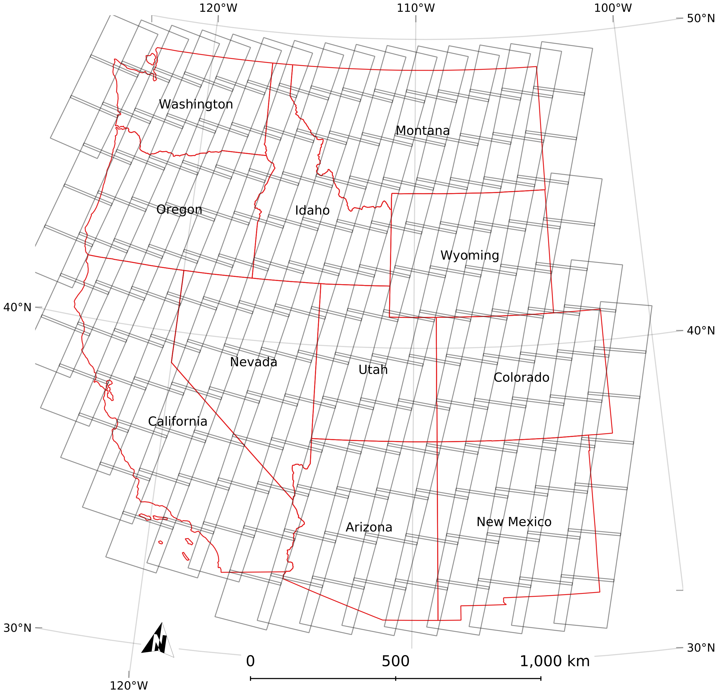
IrrMapper uses a RF modeling approach to predict four land classes of irrigated agriculture, dryland agriculture (i.e., crops receiving water only from precipitation), uncultivated lands, and wetlands at an annual time step, and at 30-m spatial resolution across the Western U.S. The RF model is parameterized using a large set of training data of both the target class (i.e., irrigation) and non-target classes (e.g., uncultivated), and numerous geospatial and climatic datasets. The training data consist of manually developed Geographic Information System (GIS) field boundary polygons and attributes of irrigation-equipped and unirrigated lands developed by numerous state and federal agencies, and research institutions. Input parameter data are geospatial and climate datasets including Landsat and aerial imagery, terrain and land use data, and precipitation, temperature, and evaporative demand (see Supplementary Material). We sampled 132 parameter values from geospatial and climate datasets at 60,000 randomly distributed training points within our field polygon training dataset, and used them to train and apply the RF algorithm to predict and perform accuracy assessment of irrigation status classes across the Western U.S. We used Google Earth Engine (GEE [62]), a cloud-based geospatial analysis platform and multi-petabyte catalog of geospatial data and satellite imagery to access all imagery used in training data development, compile all model input data, to parameterize and train the RF model, to predict land class, and to extract results and validation data. All services from GEE were free.

2.2. Study Area

The study area consists of 11 Western U.S. states of Arizona, California, Colorado, Idaho, Montana, New Mexico, Nevada, Oregon, Utah, Washington, and Wyoming, an area of 3.1 million km 2 (Figure 1). This region is more arid than the eastern U.S. with exceptions in the Pacific Northwest and regions of northern California. Annual precipitation in the study area ranges from a minimum of approximately 60 mm year 1 in southeast California to over 3000 mm year 1 in the Cascade Mountains of Washington. Evaporative demand ranges from approximately 500 mm year 1 in the Cascade Mountains of Washington to over 2600 mm year 1 in southern Nevada. The Southwest U.S. is dominated by summer monsoonal precipitation, while the northern and Pacific zones receive the majority of precipitation in the winter, much of it in the form of snow. In general, the climate transitions from Pacific coastal and Mediterranean to continental, from west to east.

2.3. Landsat and Aerial Imagery

We extracted 132 parameters to use as input data to the model exclusively from datasets with continuous coverage of the entire study region and study period. The 30 m resolution Landsat data used in this work provides six optical bands collected from the Landsat TM, Landsat 7 ETM+, OLI sensors: red, green, blue, near infrared, and two shortwave infrared bands. We used the Landsat Collection 2 Surface Reflectance product, the highest level of processing currently available. Landsat 5 TM and Landsat 7 +ETM surface reflectance data have been corrected for atmospheric conditions and viewing angle geometry using the Landsat Ecosystem Disturbance Adaptive Processing System (LEDAPS [63]) algorithm. Landsat 8 OLI surface reflectance data were processed using the Land Surface Reflectance Code (LaSRC [64]). For each year, we calculated the mean surface reflectance for each of the six optical bands for four periods: March 1–May 1; May 1– July 1; July 1–September 1; and September 1–November 1. We also calculated the maximum, minimum, and mean per-pixel Normalized Difference Vegetation Index (NDVI) for each year. We did not attempt to perform a radiometric cross-calibration between Landsat instruments; differences between processed surface reflectance images exist but are small [65].
Our study area consists of 186 Landsat path-row scenes (Figure 1), each of which was revisited every 16 days by each Landsat mission during the study period. Simultaneous operation of Landsat 5 and 7 from 1999 to 2012 and Landsat 7 and 8 from 2013 yields an 8-day revisit time during 20 years of our 33-year study period, a total of 269,241 available scenes. In May 2003, Landsat 7 suffered a scan line corrector hardware failure (SLC-off) resulting in data gaps in image captures covering about 20% of the image area [66]. While the multiple concurrent Landsat operations during most of our study period allowed for data collection everywhere, during the 2012 collection period, only Landsat 7 SLC-off data were available.
We used images from the U.S. Farm Service Agency National Aerial Imaging Program (NAIP) to verify agricultural field boundary accuracy. NAIP provides 3- and 4-channel (i.e., Red–Blue–Green and Red–Blue–Green–Near Infrared) imagery at various resolutions (0.6, 1, and 2 m) from 2003 to present, offered on a state-by-state basis for multiple years. We used the latest available imagery for each state in our data development process, see [67].

2.4. Meteorology and Climate Data

The University of Idaho Climatology Lab produced daily surface Gridded Meteorology (gridMet) at 4-km resolution for the conterminous U.S. from 1979 to present [68]. We extracted mean temperature and total precipitation from gridMet for the duration of the four growing season periods and for the preceding water year (i.e., October 1–September 30) to the termination of each of the growing season periods, for each year covered in our training data (28 years). We also extracted the 10th, 50th, and 90th percentile annual minimum and maximum temperature, the annual total precipitation, and the annual total potential evapotranspiration from gridMET. We extracted minimum, maximum, and average monthly temperatures and monthly average precipitation for each month of the calendar year from WorldClim, a 1 km resolution worldwide gridded climate product providing 30-year climate normals based on the period 1970–2000 [69].

2.5. Terrain and Land Use Data
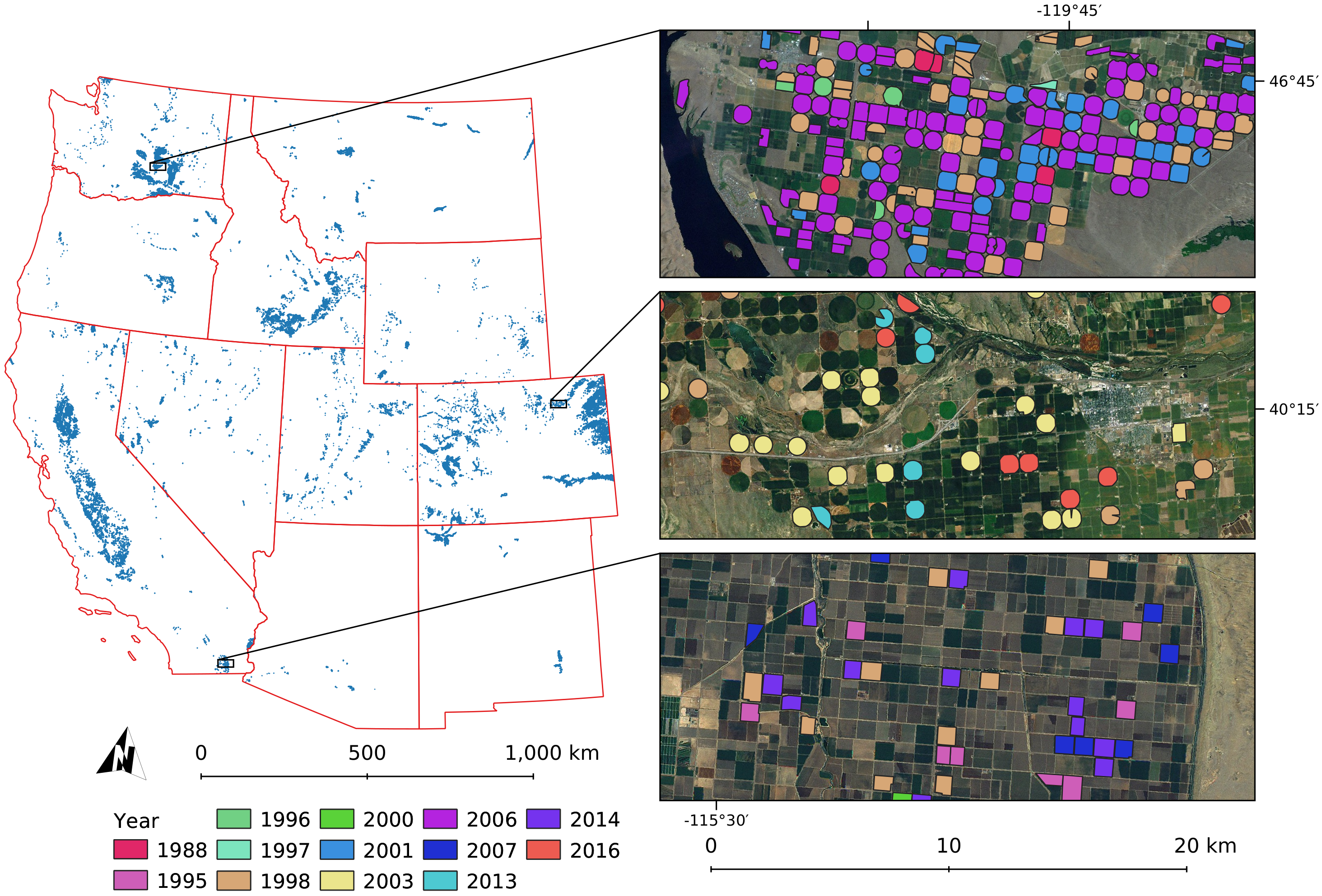
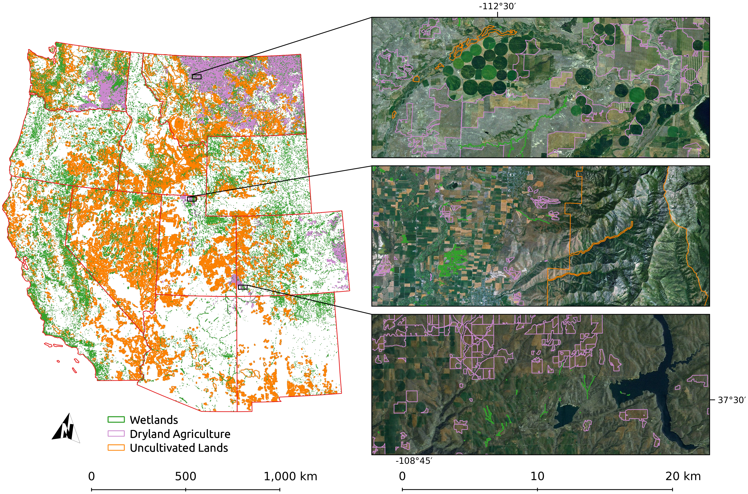
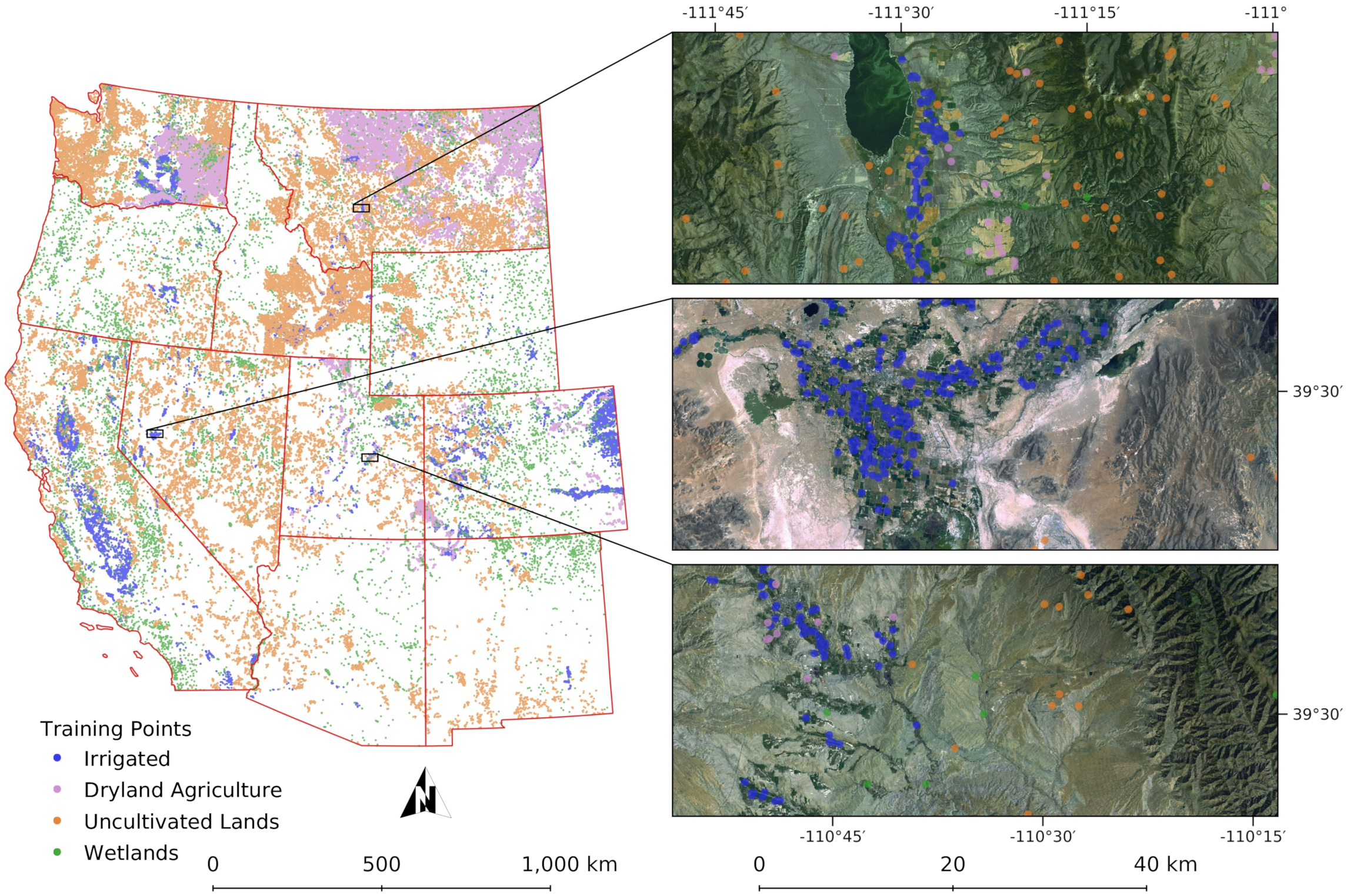
We extracted elevation, slope, and aspect from the USGS National Elevation Dataset 1 3 arc-second resolution digital elevation model (DEM). Using the DEM we calculated the Topographic Position Index at 150, 250, and 1250 m [70]. We used the USDA Crop Data Layer [71] and the the USGS National Landcover Dataset [72] to generate binary crop mask and land cover layers.

2.6. Training Data

The training and validation datasets for IrrMapper were derived from polygon vector data covering partial areas of each state, obtained from federal and state agencies, and research institutions (Table 1). All data were stripped of attribution and joined into a database; only geometries were used. Four land classes were represented in the training data: irrigated agricultural fields (Figure 2), dryland agricultural fields, uncultivated lands, and wetlands (Figure 3).
We assumed the dryland agriculture, wetlands, and uncultivated lands were constant throughout our study period of 1986–2018. We attributed irrigation to irrigation-equipped fields during specific years to account for the possibility that irrigation-equipped fields were fallowed during some years (Table 1).
Irrigation-equipped polygon datasets that had been developed for specific time periods were verified for those years. Irrigation-equipped polygon datasets without temporal information were generally developed for 4–6 years. These years were chosen to represent a range of climatic variability within the study period found using the Climate at a Glance tool [88], with at least one year of below normal water year precipitation, at least one year of above normal water year precipitation, and at least one year of near-normal water year precipitation (Figure 4).
Irrigation training data development consisted of two steps: (1) filtering the polygons by NDVI, a common satellite-detected proxy for vegetation density and vigor; and (2) visual inspection. Our filter kept the polygons containing pixels where the lower 15th percentile NDVI of pixels had maximum NDVI greater than 0.5 during either the early or the late summer, May to July and July to October, respectively. Polygons that did not meet the criteria of the filter were ignored. We inspected all polygons resulting from the filtering process using NAIP aerial imagery and Landsat 5, 7, or 8, early, late, and overall summer maximum NDVI. We compared the NDVI with the surrounding natural vegetation and removed any polygons with only partially irrigated extent or where the field boundaries were inaccurate. Our verified irrigation dataset consists of 101,875 features, each corresponding to the year for which it was filtered and then inspected, of which 53,367 are unique agricultural field boundaries covering 14,659 km 2 (1.9% of total training data area). The 48,508 duplicates are fields that were found to be irrigated for more than one year during the years we selected for data development in the state. To our knowledge, this represents an unprecedented collection of verified irrigated areas.
The dryland agriculture training data is almost entirely within the major wheat-growing regions of CO, MT, and WA, with a small amount in the Upper Colorado River Basin in WY, UT, AZ, and CO. The features represent cultivated lands lacking irrigation infrastructure. The dryland data consists of 38,259 fields covering 63,406 km 2 (10.4% of total training data area). These data were inspected for general accuracy using NAIP imagery at several locations but were not systematically verified on a field-by-field basis. The wetlands training data were collected from the U.S. Fish and Wildlife National Wetlands Inventory [75]. We chose 99,697 features at random from the ‘Freshwater Emergent Wetland’, ’Freshwater Forested/Shrub Wetland’, and ‘Riverine’ classes, covering 2343 km 2 (0.4% of total training data area). The uncultivated class was composed of the USDA Forest Service Roadless Areas Inventory [73], the National Wilderness Preservation System wilderness inventory (comprised of wilderness areas managed by the Bureau of Land Management, Fish and Wildlife Service, Forest Service and National Park Service) [74], and sources of forestry and rangeland data gleaned from states. The uncultivated dataset consists of 39,409 features covering 534,442 km 2 (87.4% of total training data area). As with the dryland data, the wetlands and uncultivated lands data were inspected to ensure general accuracy, but not systematically verified. We used all the appropriate training data we were able to obtain. The four classes of training data together cover 611,514 km 2 , about 20% of the study region.

2.7. Model Training and Classification

IrrMapper is trained using the Random Forest (RF) algorithm, a non-parametric ensemble decision tree classification and regression algorithm. RF chooses random subsets of training samples to train many decision trees and makes a classification based on the mode of the set of trees. In the IrrMapper RF, model hyperparameters were tested using the Scikit-Learn Python implementation of the RF algorithm on our training dataset [89]. We set the number of Rifle decision trees to 100, the number of variables per split to 11, the minimum size of the terminal node to 1, and deactivated the out-of-bag mode in favor of testing accuracy using cross-validation (see below). We then used our hyperparameters to run the GEE implementation of RF.
To extract training data for IrrMapper, pixel sampling locations for 30,000 points within the irrigated areas and 10,000 points within each unirrigated class were placed randomly within a 20-m interior buffered extent of the vector coverage for each land class over the study area (Figure 5). The points within the irrigated coverage were attributed with the year for which that field polygon had been verified as irrigated, while the other classes were randomly assigned a year from the 28 years we had irrigation training data. We used GEE to then create a composite image of both static (i.e., land cover, terrain, and climate) and dynamic (i.e., Landsat, Landsat-derived indices, and meteorology) gridded data. Each pixel value was extracted for each sample point and returned in a table for use in training the RF algorithm. We trained the RF algorithm within GEE and predicted land class using the 132-layer stack of input rasters over the entire study area each year 1986–2018. While IrrMapper is trained and predicts using four land cover classes, in a final processing step, the three unirrigated land classes are grouped into a general ‘unirrigated’ class, to give a binary irrigated/unirrigated classification result over the study region. To assess variable importance, we ran the Scikit-Learn implementation of the RF model using our IrrMapper hyperparameters over ten iterations to extract the average feature importance of our model parameters.

2.8. Model Cross Validation

To validate our GEE-based IrrMapper RF model, we extracted a sample set of 60,000 points using the same procedure as described above for training points extraction. Points located within a 60-m buffer of the original training dataset were removed. A random subset of 10,000 points from each class was then used to extract results from GEE and calculate a confusion matrix. Additionally, a random subset of points, the number of which for each class was weighted according to the relative area of each of the training classes, was selected for use in further assessment as discussed below. This provided a dataset for a spatially independent cross-validation and allowed us to use the maximum quantity of data in GEE to train the RF without holdouts.

2.9. Comparison with National Agricultural Statistics Service Data

For comparison purposes, we compiled Census of Agriculture data for 1987–2017 to find semi-decadal, county-level irrigated area. We aggregated data for years 1987, 1992, and 1997 from [90] and years 2002, 2012, and 2017 from Quick Stats [2]. To remove outliers in our comparison of NASS data with IrrMapper, we masked any pixel location where irrigation was detected for less than five years over the 33-year study period.

2.10. Calculation of Irrigated Area Change

To capture change in irrigated area over the course of the study period, we processed ‘early’ and ‘late’ irrigation-equipped masks. These masks represent areas where irrigation was detected during at least two of the five-year periods at the beginning and the end of the study period. We resampled these rasters to a 4-km resolution grid and calculated the change in irrigated area per 16 km 2 pixel.

3. Results

IrrMapper consists of 33 annual, 30-m resolution maps of the binary classification of irrigation status of the western 11 states, 1986–2018. We used GEE to train the RF and predict over the entire study region annually, producing a GEE Image Collection of 33 maps at 30 m resolution. Computation time for training and prediction was about 60 h (Figure 6).

3.1. Model Accuracy

Using 40,000 points for cross validation, we found an overall binary classification accuracy of 97.8% for classification of irrigated vs. unirrigated lands at the validation point locations. False positive prediction of unirrigated land as irrigated by IrrMapper dominated the model error, accounting for 88% of false classifications. IrrMapper has some limitations in discriminating between non-agricultural classes and shows a high level of confusion between the wetland and uncultivated lands classes in the validation data (Table 2). We found an overall accuracy of wetland vs. uncultivated classification by IrrMapper of 88.2%. Wetlands classification in terms of producer’s accuracy was the lowest of the four classes at 77.1%. IrrMapper discriminates with a high level of accuracy between irrigated and dryland classes, however, and has an overall irrigated vs. dryland classification accuracy of 99.1%. IrrMapper had producer’s accuracy of 98.9% and 96.6% for irrigated and dryland classes, respectively.
The limitations of the IrrMapper training data caused by the limited geographic extent of irrigated areas in our training data become apparent when the cross validation data are grouped into binary classes (i.e., irrigated and unirrigated) and weighted for the relative area of each training dataset (Table 3). While the overall accuracy of the weighted cross validation dataset is 98.6%, a small number of false positive classifications of unirrigated lands led to a low producer’s accuracy of 57% for the irrigated class.

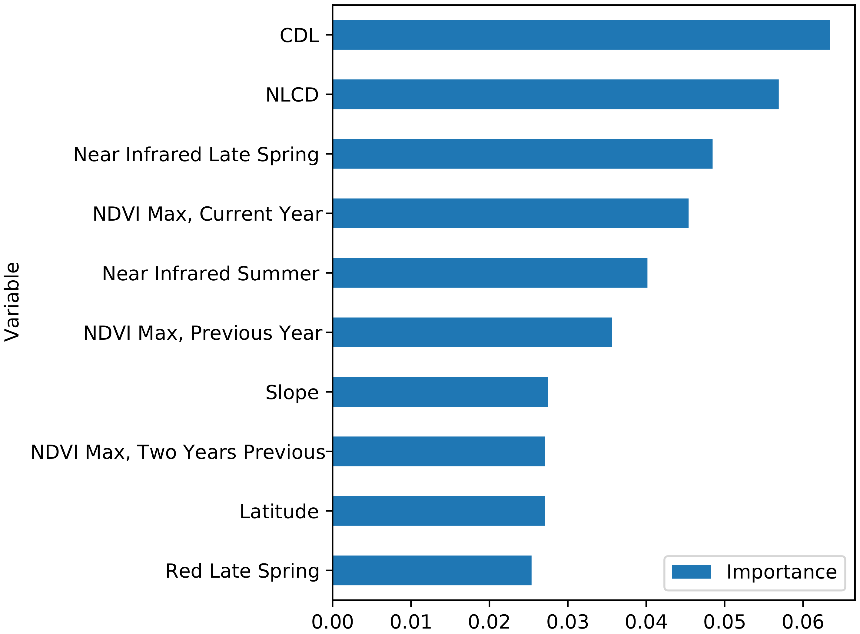
3.2. Variable Importance

Of the 132 parameters used in the study, the ten most important, in descending order, are CDL classification, NLCD classification, late summer near infrared, mid-summer near infrared, calendar year maximum NDVI, previous year maximum NDVI, latitude, terrain slope, two year’s previous maximum NDVI, and mid-summer red (Figure 7).

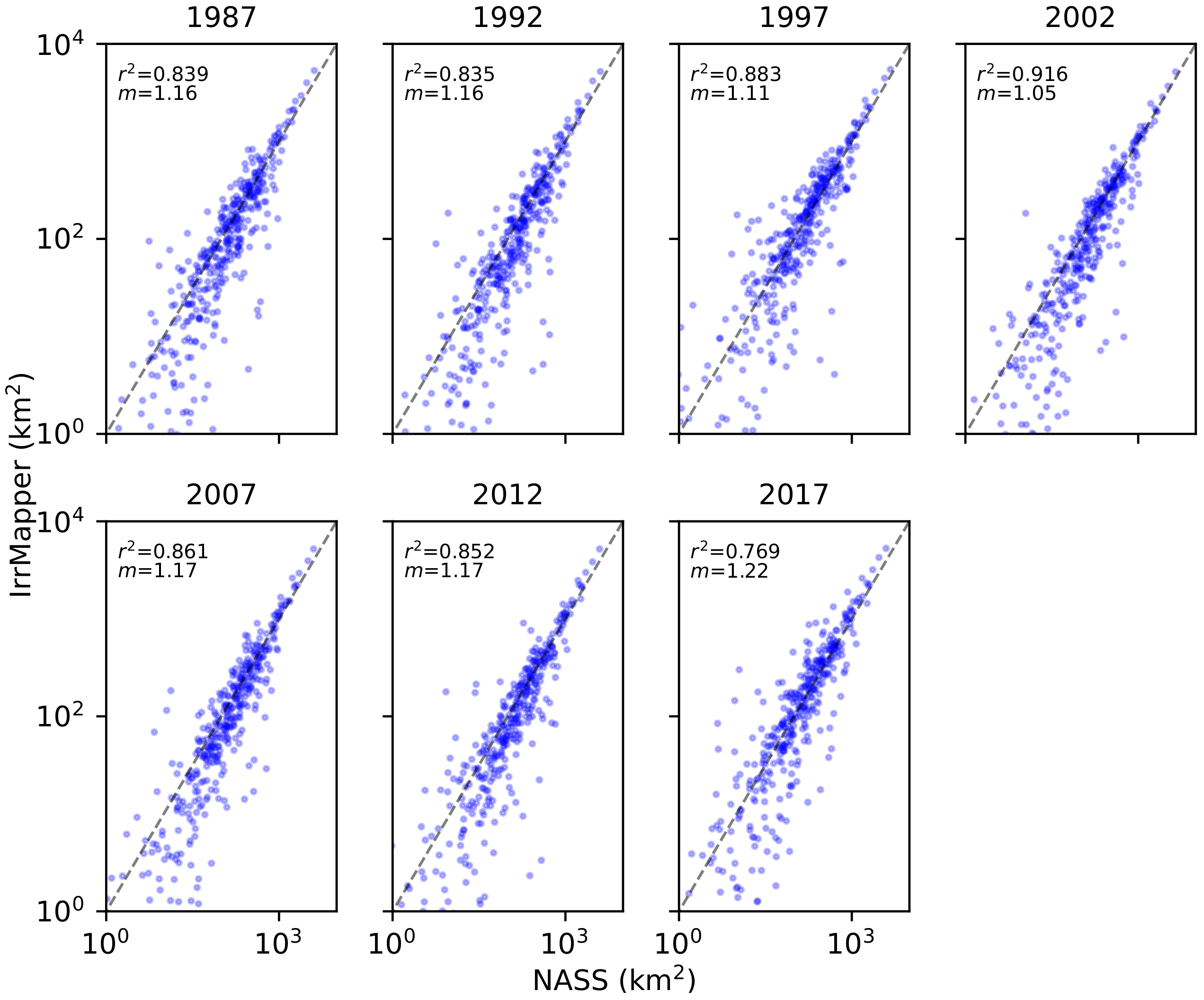
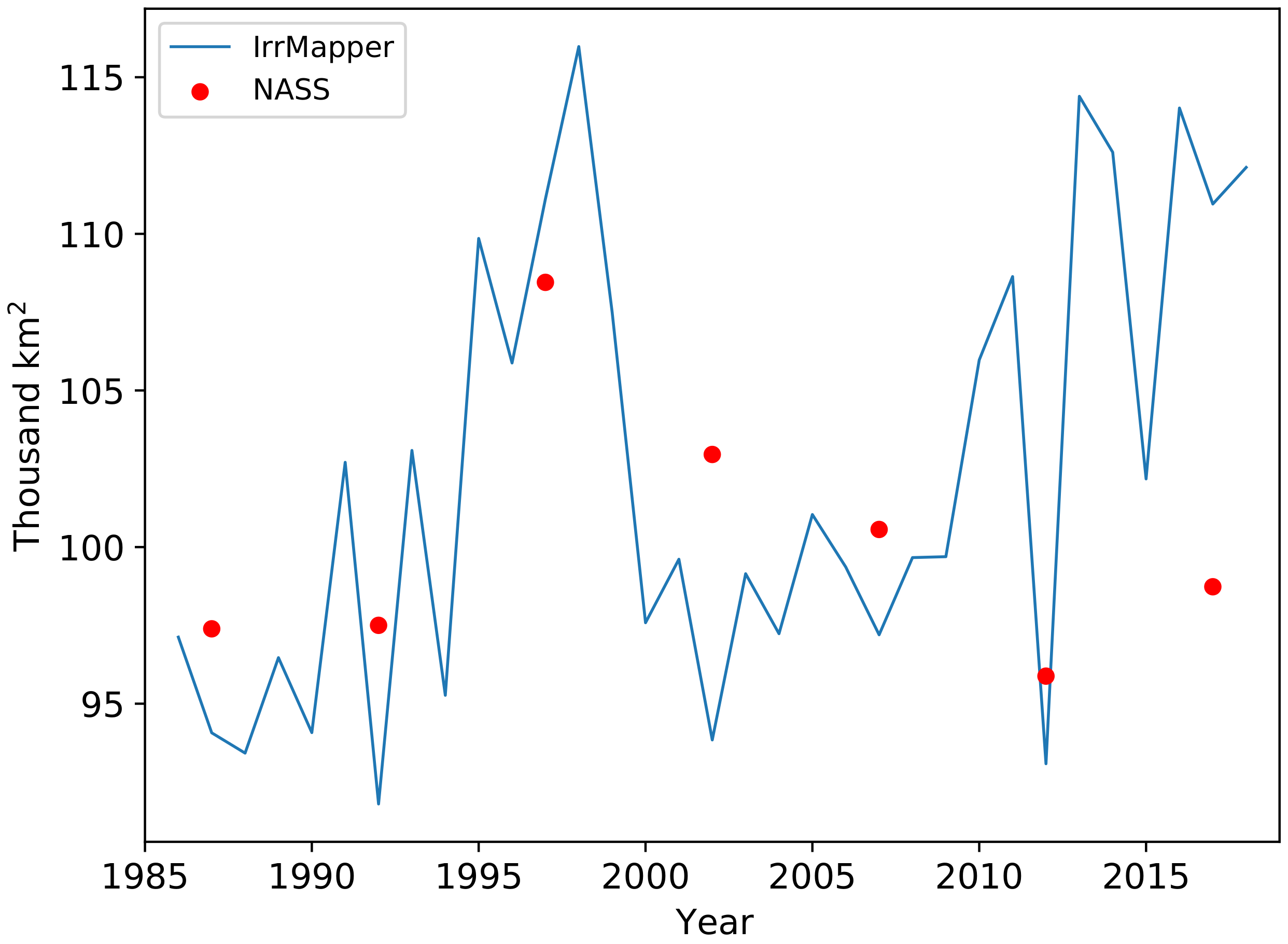
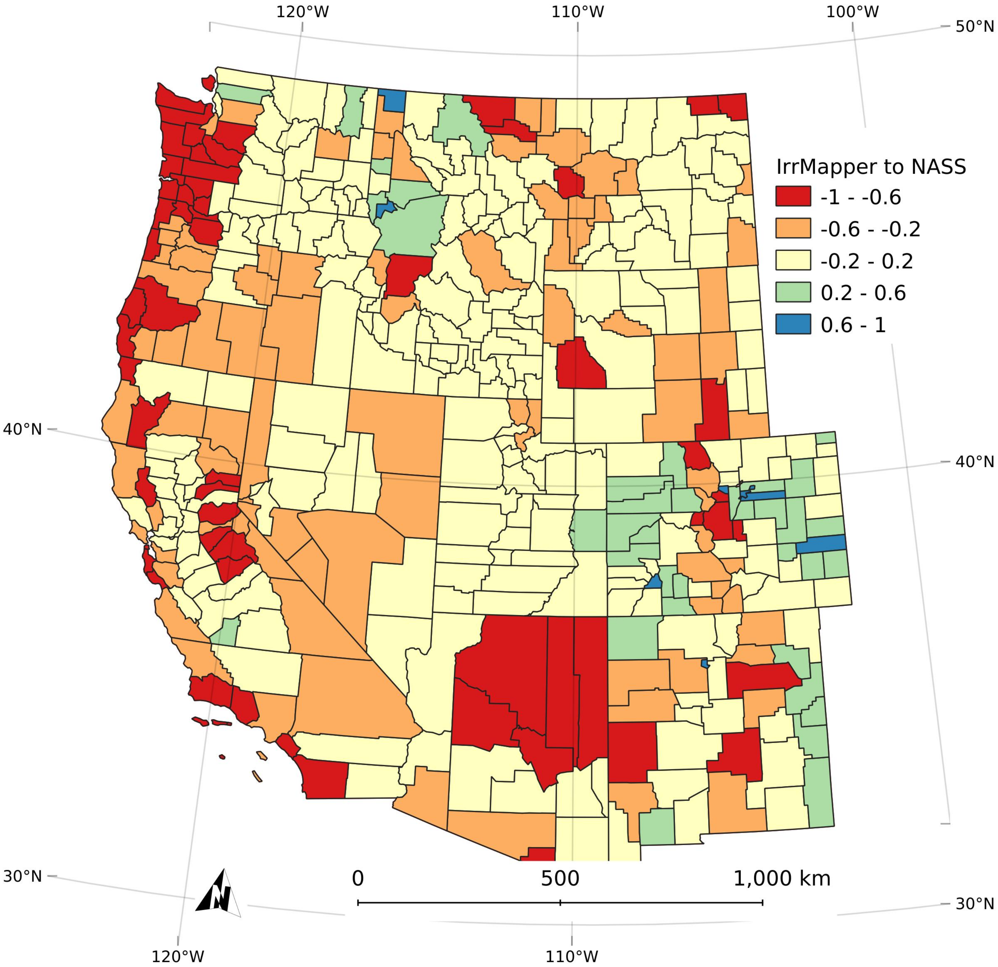
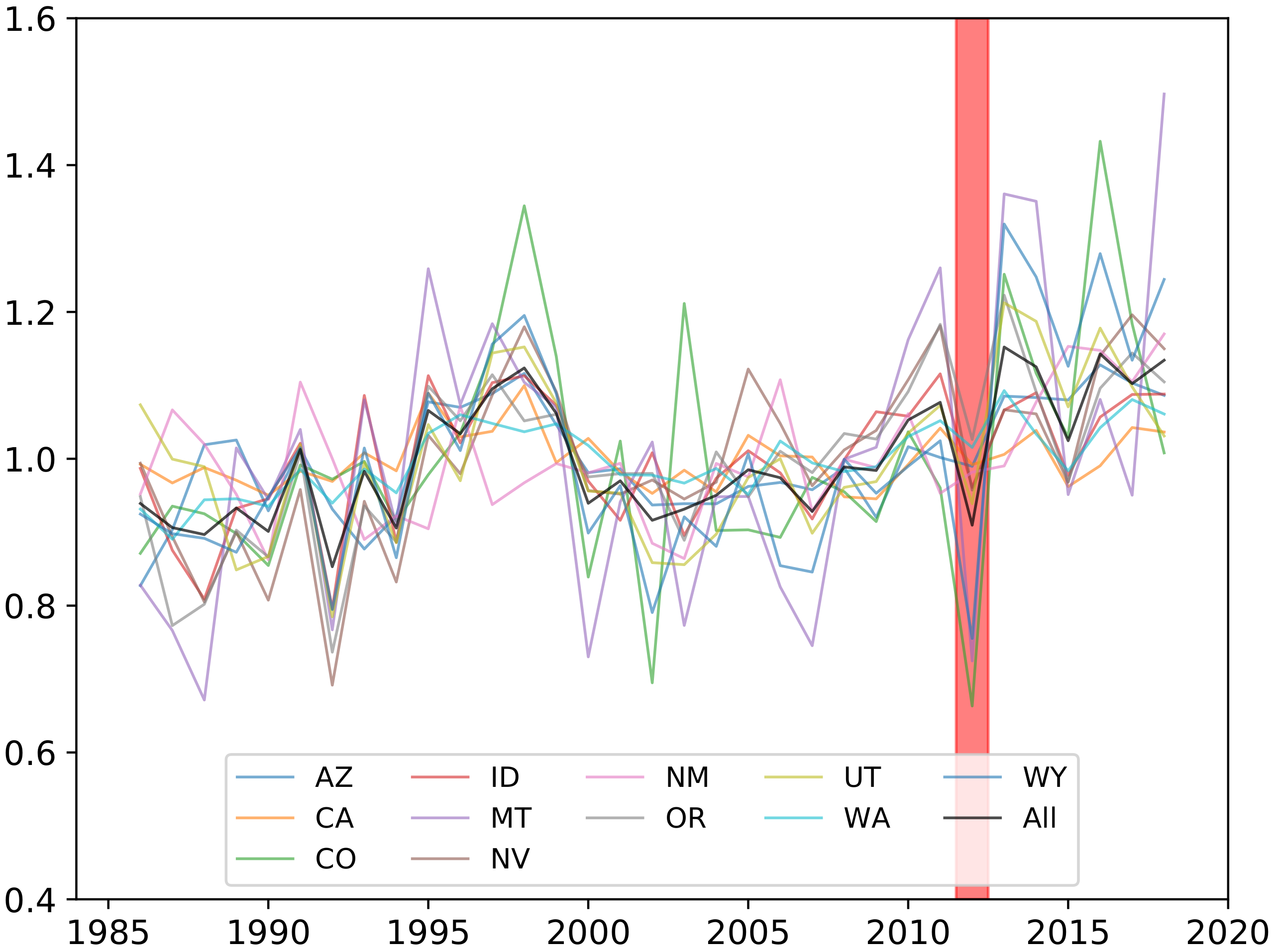
3.3. Comparison with NASS Data

IrrMapper shows good agreement with the NASS agricultural statistics (Quick Stats) at the state scale and for counties with high irrigated area (Figure 8 and Figure 9). Counties with low NASS-reported irrigated area have large relative differences with IrrMapper. Statewide estimates of irrigation matched well with NASS reported statistics over the seven years of available data from NASS (r 2 = 0.94). The county NASS data and IrrMapper had a lower level of agreement (r 2 = 0.90). IrrMapper and NASS show general agreement on the study area trends over the study period; both show relatively low irrigated area at the beginning of the study, a peak in the late 1990s, and increasing irrigation toward the end of the study (Figure 9).
IrrMapper tends to make lower estimates of irrigated area along the Pacific coast and in semi-arid areas where irrigation density is low (Figure 10). IrrMapper tends to make higher estimates of irrigated area in counties with urban centers and counties on the eastern plains. The best overall agreement between IrrMapper and NASS was found in the states of Idaho and Utah.

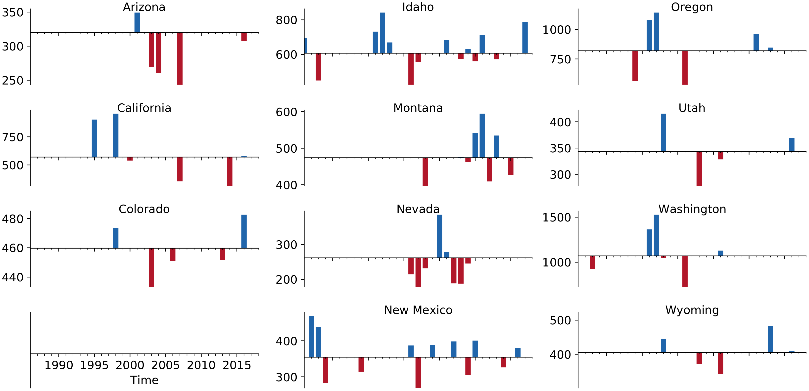
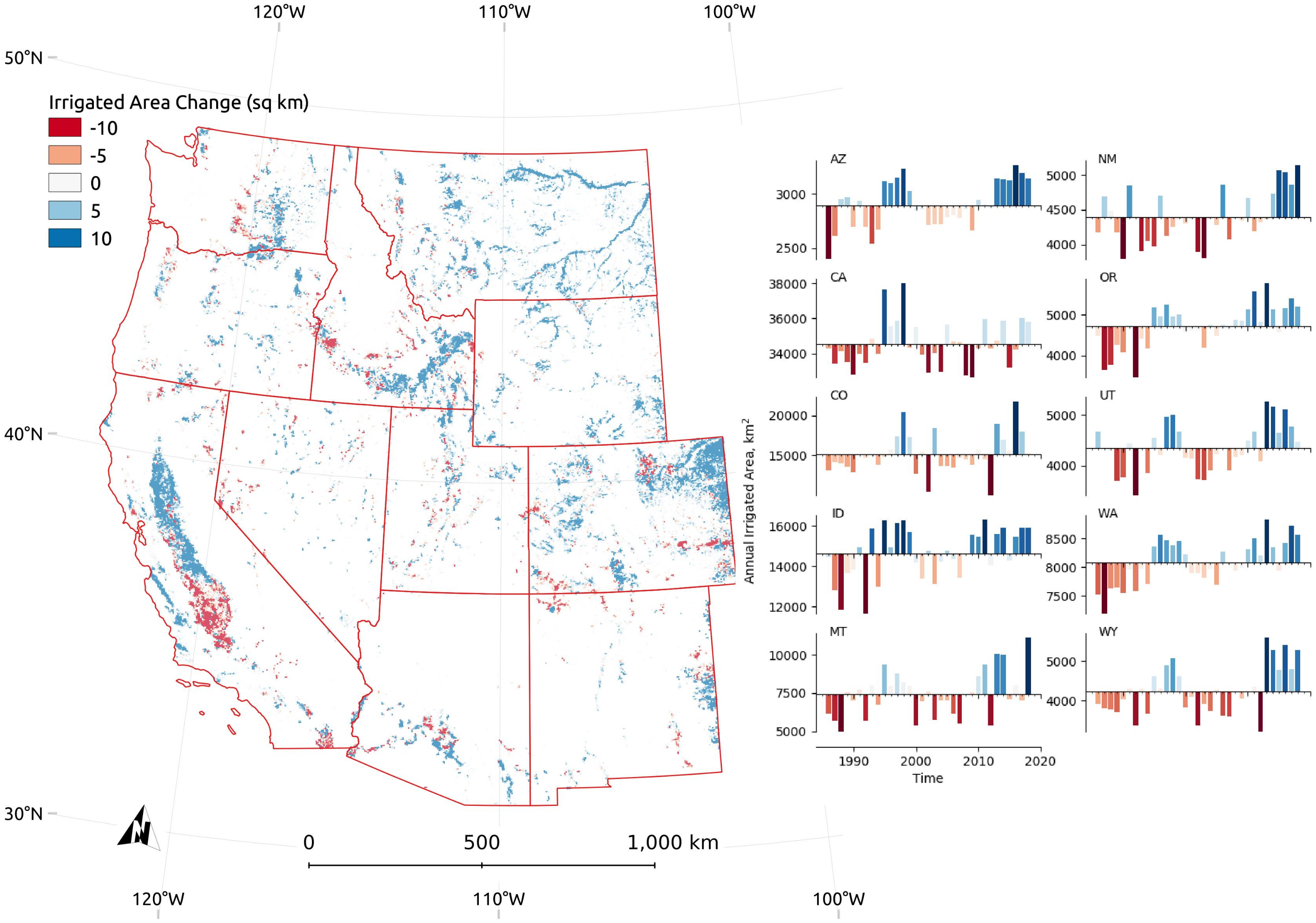
3.4. Trends in Irrigation

IrrMapper detected a general increase in total irrigated area over the course of the study period of 15.4%, from 97,100 km 2 in 1986 to 112,100 km 2 in 2018, with the maximum irrigated area reaching 116,100 km 2 in 1998, and the minimum irrigated area of 91,900 km 2 in 1992 (Figure 9). State-by-state trends of normalized irrigated area show that Colorado and Montana had the largest fluctuations in irrigated area with standard deviation of 2465 and 1494 km 2 , respectively (Figure 11). IrrMapper detected a decrease in irrigated area among all states in the study region in 2012, potentially as a result of using Landsat 7 SLC-off data.
IrrMapper shows a general increase in irrigated area in the major arid and semi-arid agricultural regions around the west, including the eastern Columbia River Basin, the Snake River Plain, eastern Colorado and New Mexico, and southern Arizona (Figure 12). Notable decreases in detected irrigation were found in the Treasure Valley of Idaho, the southern Central Valley in California, and the western slope of the Columbia River Basin.

4. Discussion

Results of this study show IrrMapper classifies irrigated areas with a high degree of accuracy when tested on a spatially independent validation dataset (Table 2). Overall accuracy of IrrMapper in terms of irrigated vs. unirrigated classification (97.8%) is higher than comparable maps (MIrAD-US, 92%; LANID, 94%; and HPA, 91.4%). The skill of IrrMapper classification suggests the selected input data has a strong correlation with each of the target classes, and demonstrates the suitability of most predictive variables, i.e., land cover, Landsat satellite data, geographic location, and terrain (Figure 7). Further, IrrMapper validation results (Table 2) suggest the inclusion of training data from a vast representation of geographic locations, climate conditions, and meteorological scenarios enables high-accuracy classification over the extremely varied spatiotemporal domain of our study.
When weighted by relative area of training data, validation results suggest over-prediction of irrigation by IrrMapper (Table 3). The relative contribution of each unirrigated class to over-prediction can be inferred from Table 2, where misclassification of unirrigated land as irrigated (i.e., false positive) is much more common than the misclassification of irrigated as unirrigated (i.e., false negative). This is likely a result of both the unbalanced area of training data from each class and the unclear differentiation between irrigated areas and wetlands in the wetland training data. Over 97% of the total training data area is composed of the uncultivated and dryland classes. As these land uses represent the majority of both our training data and the study area as a whole, a low rate of false positives likely leads to a small but significant contribution to total irrigated area from unirrigated lands. This is evident in results over known uncultivated and dryland areas, where false positive classification of single or small groups of pixels is noted. This problem may be mitigated by using a noise removal technique in post-processing, as done by Deines [51]. While wetlands data represent a small fraction of the training area, during model development we found the inclusion of those data to be critical to IrrMapper’s discriminative power in riparian areas where adjacent wetlands and irrigation are common and share a similar appearance. However, inspection of our wetland data reveals areas where irrigation likely occurs as evidenced by simple diversions and ditch networks. It is often unclear in NAIP imagery where areas supplied with irrigation water end and wetlands begin. In our training data and in nature, the existence of wetlands and irrigation in the same place is possible, and therefore both semantic and physical distinction between irrigated areas and wetlands is blurred. This problem may be overcome by restricting the wetlands training data to areas where irrigation does not occur.
Comparison of county-level NASS irrigation survey data and IrrMapper results shows general agreement (r 2 = 0.90) with the best agreement in areas with more irrigation and less agreement in counties with low rates of irrigation (Figure 8). Large relative differences are expected in counties where both estimates are a small fraction of total area (e.g., the northern counties of Arizona). In urban areas with limited irrigated area, IrrMapper generally estimates greater irrigated area relative to NASS. This can be explained in part by Census of Agriculture classification of farms, where only farms expected to produce and sell more than $1000 of agricultural products are surveyed. This approach omits irrigation by golf courses, hobby farms, and playing fields, areas which are detected by IrrMapper and may represent a large portion of total irrigation in urban and desert landscapes. The bias toward false positive classification of irrigation in IrrMapper likely also contributes to larger estimates by IrrMapper in counties with extensive dryland and uncultivated lands. In areas of extensive irrigation, results are in better agreement, likely due to higher contribution to irrigation from farms included in the Census of Agriculture survey, and less unirrigated area in which IrrMapper may misclassify land type.
IrrMapper tends to make county-level estimates of irrigated area lower than NASS estimates along the Pacific coast and in arid and semi-arid counties with low density of irrigation (Figure 10). In the Pacific Northwest, the high relative contribution to crop water requirements from precipitation may allow low irrigation intensity and thus low contrast in satellite images between irrigated and unirrigated areas, and under-classification of irrigation by IrrMapper. Along the coast of Oregon and California, underestimates may be attributable to lower density of IrrMapper training data and under-classification as a result. The most notable region of generally higher IrrMapper estimates are the easternmost counties of the study area in Colorado and New Mexico. These areas likely have significant rates of false positive classification of dryland agriculture as irrigated. This may be caused by sub-annual cropping of dryland agriculture in areas where soil moisture is conserved through the use of herbicides during fallow periods and where subsequent croppings result in a high NDVI relative to adjacent, unirrigated land. Despite disagreement between the two methods, when aggregated over the study area, IrrMapper and NASS show rough agreement on trends in the extent of irrigation; both identify a peak in irrigated area in the mid-1990s, followed by a decline through the 2000s, and a rise toward the end of the study period (Figure 9). This suggests that, in addition to its capacity to accurately map irrigation at the local scale, IrrMapper also has the capacity to detect regional trends in irrigation at higher temporal resolution relative to NASS.
Spatial trends in irrigation detected by IrrMapper are complex and are likely driven by many factors, including changes in land use, timing of crop planting, crop type, water resource limitations, and changes in irrigation efficiency, and also limitations in the IrrMapper approach (Figure 12). While analysis of the drivers of changes in irrigation is outside the scope of this paper, we hypothesize several factors that deserve further investigation. We suspect the areas around Phoenix, AZ; Denver, CO; Portland, OR; Ellensburg and Yakima, WA; and Boise, ID have undergone suburban development that has replaced formerly irrigated areas. We suspect demand for fresh winter agricultural produce has driven a change in cropping time from summer to winter in southern California, a period for which IrrMapper is not designed to detect irrigation (see below). We suspect demand for orchard and vineyard crops has led to an increase in their extent. IrrMapper may not detect them due to bias in the training data development toward selection of irrigated fields with high maximum summer NDVI (see below), and that irrigation of vineyards and orchards may drive a weaker NDVI response due to crop spacing. We suspect formerly irrigated areas in Nevada, Colorado, and New Mexico have been retired due to legal and physical limits on water availability. Widespread increases in irrigated area may be due to irrigation development, and use of more efficient irrigation application equipment and thus expansion of irrigated area despite constant rates of water extraction. Deines et al. [50] studied changes in irrigation over the High Plains Aquifer; previous-year commodity price was found to be positively correlated to irrigated area, while irrigation volume and depth were negatively correlated with precipitation. Such studies of the drivers and patterns of irrigation and water use in the Western U.S. may be enabled in the future by IrrMapper.
IrrMapper limitations are likely due to its simple model parameterization and bias in the training data development process. A central assumption of IrrMapper is that the irrigation occurs during the March–November time period. The assumption that the growing season occurs between March 1 and November 31 may contribute to under-classification of irrigation in areas with a winter growing season. This is apparent in areas such as the southern Central Valley and Imperial Valley in California and Yuma, AZ, which have seen decreases in irrigated area according to IrrMapper (Figure 12). We ran a sub-model ‘IrrMapper LCRB’ for the Lower Colorado River Basin, and found that when the growing season is extended to the entire year, IrrMapper detects more irrigated fields. This suggests IrrMapper may benefit from customized parameterization within specific regions. Further, IrrMapper does not explicitly model the temporal dynamics of the Landsat spectral signal. IrrMapper uses the mean surface reflectance for each growing season period and thus information on the spectral dynamics of each location within that period is lost. Including temporal data associated with specific image captures may improve IrrMapper’s ability to discriminate between land classes that experience distinct temporal dynamics in spectral response through the year, but have similar spectral means.
While the geometry of the fields was created by experts, the filtering process depended only on a set of NDVI statistics. This approach may systematically exclude areas that are sparsely irrigated and show a weak NDVI response, adding bias to the model. An effort was made to represent various land types, including those with weaker NDVI signal (e.g., vineyards and widely spaced orchards), but, in some cases, irrigated fields were removed from the data because the field included areas that were not reached by the irrigation equipment. The training data are thus biased toward intense irrigation, and likely fail to detect irrigation in areas with infrequent or low-intensity irrigation. The assumption of static land cover in the unirrigated classes (i.e., dryland, wetland, uncultivated) may also introduce error in the training data where land class has changed during the study period. The assumption is probably best for the uncultivated class (e.g., national forest, roadless areas), and weakest for the dryland class, where conversion to irrigation may occur. We suspect the locations where dryland was converted to irrigated are likely limited in our training data because the geospatial data development occurred recently.
IrrMapper is an improvement over previous mapping efforts in the Western U.S. given the large geographic and temporal extent of both training data and our predictions. Further, our predictions depend only on our independently verified training data, compared to many previous efforts where irrigation models have depended on agricultural census data to parameterize models using spectral thresholds (e.g., LANID, MIrAD-US). While these models effectively leverage the predictive power of irrigated areas’ spectral signature, they rely on agricultural statistics and therefore incorporate both the error in the survey and irrigated areas excluded from the tabulation according to the criteria of the agricultural survey. Further, they may not be suited to generalization in time, as the conditions during census years may not be representative of regional climatic variability. Models that ‘tune’ to the agricultural statistics during only one or several growing seasons may mistake irrigation status when the model is applied to the same place under different climate or economic scenarios [4,91]. As the training data used in IrrMapper represent the wide range of climatic, spatial, and temporal variability we observe in the West, the model can be relied on to make good predictions for years without training data. Further, IrrMapper uses existing land use classification models (i.e., NLCD and CDL) as input parameters, rather than as training data or as a mask for areas not considered agricultural land by those model products (AIM-HPA, LANID, and MIrAD-US). This allows the model to determine the relative importance of these parameters, rather than using them as a mask and thus incorporating the error inherent in the land use data into the map. IrrMapper is created independently of the NASS agricultural statistics, and can thus be used as an independent comparison to examine both existing irrigation maps and historic agricultural census data.

5. Conclusions

Water resources management in the Western U.S. requires accurate, timely, and high resolution irrigation maps. These maps are a critical resource in assessing the impact of irrigation on human and ecological systems and quantifying irrigated water consumption. Despite the critical importance of irrigation, the high spatial and temporal resolution mapping of its occurrence is currently lacking. IrrMapper introduces the high resolution mapping of irrigation annually, 1986–2018, over the Western U.S. Using IrrMapper, we found that irrigated area in our study region has ranged from 91,900 km 2 in 1992 to 116,100 km 2 in 1998. Irrigation increased by about 15% over the study period, from 97,100 km 2 in 1986 to 112,100 km 2 in 2018. We found that IrrMapper compares favorably with NASS agricultural census data, especially in areas of high irrigation density. IrrMapper differs most from NASS census data along the Pacific Coast, the eastern margin of the study area in Colorado and New Mexico. IrrMapper demonstrates the ability of a RF-based method to accurately map irrigation at a sub-continental scale. Future work should use a temporal parameterization and investigate the underlying drivers of change in irrigated area in the Western U.S.

Supplementary Materials

The following are available online at https://www.mdpi.com/2072-4292/12/14/2328/s1.

Author Contributions

Conceptualization, D.K. and F.M.; methodology, D.K.; software, D.K. and M.O.J.; validation, D.K.; data curation, D.K. and J.H.; writing—original draft preparation, D.K.; writing—review and editing, D.K., K.J., M.P.M., J.H., and F.M.; supervision, K.J. and J.H.; funding acquisition, K.J., J.H., and D.K.; All authors have read and agreed to the published version of the manuscript.

Funding

This research was primarily funded by the National Science Foundation under Grant No. 1633831, the University of Montana BRIDGES Fellowship. Additional funding was provided by the Montana Climate Office and the OpenET project (https://etdata.org/). Development of OpenET is supported by the S.D. Bechtel, Jr. Foundation; the Gordon and Betty Moore Foundation; the Walton Family Foundation; the Windward Fund; the Water Funder Initiative; the North, Central, and South Delta Water Agencies, and the NASA Applied Sciences Program Western Water Applications Office. In-kind support was provided by partners in the agricultural and water management communities, Google Earth Engine, and the Water Funder Initiative.

Acknowledgments

We would like to thank Jillian M. Deines for providing software to parse Census of Agriculture data. We are grateful to Daniel Pendergraph and Heather Brighton for their geospatial analysis. We thank the funding organizations and researchers at the OpenET project for technical, logistical, and financial support of this project.

Conflicts of Interest

The authors declare no conflict of interest.

References

  1. Dieter, C.A. Water Availability and Use Science Program: Estimated Use of Water in the United States in 2015; U.S. Geological Survey: Reston, VA, USA, 2018. [Google Scholar]
  2. United States Department of Agriculture, National Agricultural Statistics. Quick Stats. 2017. Available online: https://data.nal.usda.gov/dataset/nass-quick-stats (accessed on 20 March 2019).
  3. Li, X.; Troy, T. Changes in rainfed and irrigated crop yield response to climate in the western US. Environ. Res. Lett. 2018, 13, 064031. [Google Scholar] [CrossRef]
  4. Wurster, P.; Maneta, M.; Beguería, S.; Cobourn, K.; Maxwell, B.; Silverman, N.; Ewing, S.; Jensco, K.; Gardner, P.; Kimball, J.; et al. Characterizing the impact of climatic and price anomalies on agrosystems in the northwest United States. Agric. For. Meteorol. 2020, 280, 107778. [Google Scholar] [CrossRef]
  5. Troy, T.J.; Kipgen, C.; Pal, I. The impact of climate extremes and irrigation on US crop yields. Environ. Res. Lett. 2015, 10, 054013. [Google Scholar] [CrossRef] [Green Version]
  6. Schauberger, B.; Archontoulis, S.; Arneth, A.; Balkovic, J.; Ciais, P.; Deryng, D.; Elliott, J.; Folberth, C.; Khabarov, N.; Müller, C.; et al. Consistent negative response of US crops to high temperatures in observations and crop models. Nat. Commun. 2017, 8, 1–9. [Google Scholar] [CrossRef] [Green Version]
  7. Sacks, W.J.; Cook, B.I.; Buenning, N.; Levis, S.; Helkowski, J.H. Effects of global irrigation on the near-surface climate. Clim. Dyn. 2009, 33, 159–175. [Google Scholar] [CrossRef] [Green Version]
  8. Yang, B.; Zhang, Y.; Qian, Y.; Tang, J.; Liu, D. Climatic effects of irrigation over the Huang-Huai-Hai Plain in China simulated by the weather research and forecasting model. J. Geophys. Res. Atmos. 2016, 121, 2246–2264. [Google Scholar] [CrossRef] [Green Version]
  9. Yang, Z.; Dominguez, F.; Zeng, X.; Hu, H.; Gupta, H.; Yang, B. Impact of irrigation over the California Central Valley on regional climate. J. Hydrometeorol. 2017, 18, 1341–1357. [Google Scholar] [CrossRef] [Green Version]
  10. Yang, Z.; Qian, Y.; Liu, Y.; Berg, L.K.; Hu, H.; Dominguez, F.; Yang, B.; Feng, Z.; Gustafson, W.I., Jr.; Huang, M.; et al. Irrigation Impact on Water and Energy Cycle During Dry Years Over the United States Using Convection-Permitting WRF and a Dynamical Recycling Model. J. Geophys. Res. Atmos. 2019, 124, 11220–11241. [Google Scholar] [CrossRef]
  11. Sterling, S.M.; Ducharne, A.; Polcher, J. The impact of global land-cover change on the terrestrial water cycle. Nat. Clim. Change 2013, 3, 385–390. [Google Scholar] [CrossRef]
  12. Reisner, M. Cadillac Desert: The American West and Its Disappearing Water; Penguin Books: London, UK, 1993. [Google Scholar]
  13. Peck, D.E.; Lovvorn, J.R. The importance of flood irrigation in water supply to wetlands in the Laramie Basin, Wyoming, USA. Wetlands 2001, 21, 370–378. [Google Scholar] [CrossRef]
  14. Stanley, D.J.; Warne, A.G. Nile Delta: Recent geological evolution and human impact. Science 1993, 260, 628–634. [Google Scholar] [CrossRef] [PubMed]
  15. Pitman, M.G.; Läuchli, A. Global impact of salinity and agricultural ecosystems. In Salinity: Environment-Plants-Molecules; Springer: Berlin/Heidelberg, Germany, 2002; pp. 3–20. [Google Scholar]
  16. Essaid, H.I.; Caldwell, R.R. Evaluating the impact of irrigation on surface water–groundwater interaction and stream temperature in an agricultural watershed. Sci. Total. Environ. 2017, 599, 581–596. [Google Scholar] [CrossRef] [PubMed]
  17. Haacker, E.M.; Kendall, A.D.; Hyndman, D.W. Water level declines in the High Plains Aquifer: Predevelopment to resource senescence. Groundwater 2016, 54, 231–242. [Google Scholar] [CrossRef] [PubMed]
  18. Ritzema, H.; Satyanarayana, T.; Raman, S.; Boonstra, J. Subsurface drainage to combat waterlogging and salinity in irrigated lands in India: Lessons learned in farmers’ fields. Agric. Water Manag. 2008, 95, 179–189. [Google Scholar] [CrossRef]
  19. Scanlon, B.R.; Jolly, I.; Sophocleous, M.; Zhang, L. Global impacts of conversions from natural to agricultural ecosystems on water resources: Quantity versus quality. Water Resour. Res. 2007, 43. [Google Scholar] [CrossRef] [Green Version]
  20. Skaggs, R.W.; Breve, M.; Gilliam, J. Hydrologic and water quality impacts of agricultural drainage. Crit. Rev. Environ. Sci. Technol. 1994, 24, 1–32. [Google Scholar] [CrossRef]
  21. Kendy, E.; Bredehoeft, J.D. Transient effects of groundwater pumping and surface-water-irrigation returns on streamflow. Water Resour. Res. 2006, 42. [Google Scholar] [CrossRef]
  22. United States Department of Agriculture, National Agricultural Statistics Service. Census of Agriculture; National Agricultural Statistics Service: Washington, DC, USA, 2007; Volume 1.
  23. Young, L.J.; Lamas, A.C.; Abreu, D.A. The 2012 Census of Agriculture: A capture–recapture analysis. J. Agric. Biol. Environ. Stat. 2017, 22, 523–539. [Google Scholar] [CrossRef]
  24. Exbrayat, J.F.; Bloom, A.A.; Carvalhais, N.; Fischer, R.; Huth, A.; MacBean, N.; Williams, M. Understanding the land carbon cycle with space data: Current status and prospects. Surv. Geophys. 2019, 40, 735–755. [Google Scholar] [CrossRef] [Green Version]
  25. Sheffield, J.; Wood, E.F.; Pan, M.; Beck, H.; Coccia, G.; Serrat-Capdevila, A.; Verbist, K. Satellite Remote Sensing for Water Resources Management: Potential for Supporting Sustainable Development in Data-Poor Regions. Water Resour. Res. 2018, 54, 9724–9758. [Google Scholar] [CrossRef] [Green Version]
  26. Pettorelli, N.; Schulte to Bühne, H.; Tulloch, A.; Dubois, G.; Macinnis-Ng, C.; Queirós, A.M.; Keith, D.A.; Wegmann, M.; Schrodt, F.; Stellmes, M.; et al. Satellite remote sensing of ecosystem functions: Opportunities, challenges and way forward. Remote Sens. Ecol. Conserv. 2018, 4, 71–93. [Google Scholar] [CrossRef]
  27. Babaeian, E.; Sadeghi, M.; Jones, S.B.; Montzka, C.; Vereecken, H.; Tuller, M. Ground, proximal, and satellite remote sensing of soil moisture. Rev. Geophys. 2019, 57, 530–616. [Google Scholar] [CrossRef] [Green Version]
  28. Shi, K.; Zhang, Y.; Qin, B.; Zhou, B. Remote sensing of cyanobacterial blooms in inland waters: Present knowledge and future challenges. Sci. Bull. 2019, 64, 1540–1556. [Google Scholar] [CrossRef] [Green Version]
  29. Dong, C. Remote sensing, hydrological modeling and in situ observations in snow cover research: A review. J. Hydrol. 2018, 561, 573–583. [Google Scholar] [CrossRef]
  30. Zeng, Q.; Wang, Y.; Chen, L.; Wang, Z.; Zhu, H.; Li, B. Inter-comparison and evaluation of remote sensing precipitation products over China from 2005 to 2013. Remote Sens. 2018, 10, 168. [Google Scholar] [CrossRef] [Green Version]
  31. Bastiaanssen, W.; Noordman, E.; Pelgrum, H.; Davids, G.; Thoreson, B.; Allen, R. SEBAL model with remotely sensed data to improve water-resources management under actual field conditions. J. Irrig. Drain. Eng. 2005, 131, 85–93. [Google Scholar] [CrossRef]
  32. Allen, R.G.; Tasumi, M.; Trezza, R. Satellite-based energy balance for mapping evapotranspiration with internalized calibration (METRIC)—Model. J. Irrig. Drain. Eng. 2007, 133, 380–394. [Google Scholar] [CrossRef]
  33. Mu, Q.; Zhao, M.; Running, S.W. MODIS global terrestrial evapotranspiration (ET) product (NASA MOD16A2/A3). Algorithm Theor. Basis Doc. Collect. 2013, 5, 1–66. [Google Scholar]
  34. Senay, G.B.; Budde, M.; Verdin, J.P.; Melesse, A.M. A coupled remote sensing and simplified surface energy balance approach to estimate actual evapotranspiration from irrigated fields. Sensors 2007, 7, 979–1000. [Google Scholar] [CrossRef] [Green Version]
  35. Anderson, M.C.; Allen, R.G.; Morse, A.; Kustas, W.P. Use of Landsat thermal imagery in monitoring evapotranspiration and managing water resources. Remote Sens. Environ. 2012, 122, 50–65. [Google Scholar] [CrossRef]
  36. Roy, D.P.; Wulder, M.A.; Loveland, T.R.; Woodcock, C.; Allen, R.G.; Anderson, M.C.; Helder, D.; Irons, J.R.; Johnson, D.M.; Kennedy, R.; et al. Landsat-8: Science and product vision for terrestrial global change research. Remote Sens. Environ. 2014, 145, 154–172. [Google Scholar] [CrossRef] [Green Version]
  37. Zhu, Z.; Wulder, M.A.; Roy, D.P.; Woodcock, C.E.; Hansen, M.C.; Radeloff, V.C.; Healey, S.P.; Schaaf, C.; Hostert, P.; Strobl, P.; et al. Benefits of the free and open Landsat data policy. Remote Sens. Environ. 2019, 224, 382–385. [Google Scholar] [CrossRef]
  38. Claverie, M.; Ju, J.; Masek, J.G.; Dungan, J.L.; Vermote, E.F.; Roger, J.C.; Skakun, S.V.; Justice, C. The Harmonized Landsat and Sentinel-2 surface reflectance data set. Remote Sens. Environ. 2018, 219, 145–161. [Google Scholar] [CrossRef]
  39. Wulder, M.A.; Loveland, T.R.; Roy, D.P.; Crawford, C.J.; Masek, J.G.; Woodcock, C.E.; Allen, R.G.; Anderson, M.C.; Belward, A.S.; Cohen, W.B.; et al. Current status of Landsat program, science, and applications. Remote Sens. Environ. 2019, 225, 127–147. [Google Scholar] [CrossRef]
  40. Döll, P.; Siebert, S. A digital global map of irrigated areas. Icid J. 2000, 49, 55–66. [Google Scholar]
  41. Siebert, S.; Henrich, V.; Frenken, K.; Burke, J. Update of the Digital Global Map of Irrigation Areas to Version 5; Rheinische Friedrich-Wilhelms-Universität: Bonn, Germany; Food and Agriculture Organization of the United Nations: Rome, Italy, 2013. [Google Scholar]
  42. Thenkabail, P.S.; Biradar, C.M.; Noojipady, P.; Dheeravath, V.; Li, Y.; Velpuri, M.; Gumma, M.; Gangalakunta, O.R.P.; Turral, H.; Cai, X.; et al. Global irrigated area map (GIAM), derived from remote sensing, for the end of the last millennium. Int. J. Remote Sens. 2009, 30, 3679–3733. [Google Scholar] [CrossRef]
  43. Xie, Y.; Lark, T.J.; Brown, J.F.; Gibbs, H.K. Mapping irrigated cropland extent across the conterminous United States at 30 m resolution using a semi-automatic training approach on Google Earth Engine. ISPRS J. Photogramm. Remote Sens. 2019, 155, 136–149. [Google Scholar] [CrossRef]
  44. Brown, J.F.; Pervez, M.S. Merging remote sensing data and national agricultural statistics to model change in irrigated agriculture. Agric. Syst. 2014, 127, 28–40. [Google Scholar] [CrossRef] [Green Version]
  45. Pervez, M.S.; Brown, J.F. Mapping irrigated lands at 250-m scale by merging MODIS data and national agricultural statistics. Remote Sens. 2010, 2, 2388–2412. [Google Scholar] [CrossRef] [Green Version]
  46. Ozdogan, M.; Woodcock, C.E.; Salvucci, G.D.; Demir, H. Changes in summer irrigated crop area and water use in Southeastern Turkey from 1993 to 2002: Implications for current and future water resources. Water Resour. Manag. 2006, 20, 467–488. [Google Scholar] [CrossRef] [Green Version]
  47. Peña-Arancibia, J.L.; McVicar, T.R.; Paydar, Z.; Li, L.; Guerschman, J.P.; Donohue, R.J.; Dutta, D.; Podger, G.M.; van Dijk, A.I.; Chiew, F.H. Dynamic identification of summer cropping irrigated areas in a large basin experiencing extreme climatic variability. Remote Sens. Environ. 2014, 154, 139–152. [Google Scholar] [CrossRef]
  48. Pervez, M.S.; Budde, M.; Rowland, J. Mapping irrigated areas in Afghanistan over the past decade using MODIS NDVI. Remote Sens. Environ. 2014, 149, 155–165. [Google Scholar] [CrossRef] [Green Version]
  49. Teluguntla, P.; Thenkabail, P.S.; Xiong, J.; Gumma, M.K.; Congalton, R.G.; Oliphant, A.; Poehnelt, J.; Yadav, K.; Rao, M.; Massey, R. Spectral matching techniques (SMTs) and automated cropland classification algorithms (ACCAs) for mapping croplands of Australia using MODIS 250-m time-series (2000–2015) data. Int. J. Digit. Earth 2017, 10, 944–977. [Google Scholar] [CrossRef] [Green Version]
  50. Deines, J.M.; Kendall, A.D.; Hyndman, D.W. Annual irrigation dynamics in the US Northern High Plains derived from Landsat satellite data. Geophys. Res. Lett. 2017, 44, 9350–9360. [Google Scholar] [CrossRef]
  51. Deines, J.M.; Kendall, A.D.; Crowley, M.A.; Rapp, J.; Cardille, J.A.; Hyndman, D.W. Mapping three decades of annual irrigation across the US High Plains Aquifer using Landsat and Google Earth Engine. Remote Sens. Environ. 2019, 233, 111400. [Google Scholar] [CrossRef]
  52. Breiman, L. Random forests. Mach. Learn. 2001, 45, 5–32. [Google Scholar] [CrossRef] [Green Version]
  53. Jones, M.O.; Allred, B.W.; Naugle, D.E.; Maestas, J.D.; Donnelly, P.; Metz, L.J.; Karl, J.; Smith, R.; Bestelmeyer, B.; Boyd, C.; et al. Innovation in rangeland monitoring: Annual, 30 m, plant functional type percent cover maps for US rangelands, 1984–2017. Ecosphere 2018, 9, e02430. [Google Scholar] [CrossRef]
  54. Colditz, R.R. An evaluation of different training sample allocation schemes for discrete and continuous land cover classification using decision tree-based algorithms. Remote Sens. 2015, 7, 9655–9681. [Google Scholar] [CrossRef] [Green Version]
  55. Tsutsumida, N.; Comber, A.J. Measures of spatio-temporal accuracy for time series land cover data. Int. J. Appl. Earth Obs. Geoinf. 2015, 41, 46–55. [Google Scholar] [CrossRef]
  56. Lebourgeois, V.; Dupuy, S.; Vintrou, É.; Ameline, M.; Butler, S.; Bégué, A. A combined random forest and OBIA classification scheme for mapping smallholder agriculture at different nomenclature levels using multisource data (simulated Sentinel-2 time series, VHRS and DEM). Remote Sens. 2017, 9, 259. [Google Scholar] [CrossRef] [Green Version]
  57. Tatsumi, K.; Yamashiki, Y.; Torres, M.A.C.; Taipe, C.L.R. Crop classification of upland fields using Random forest of time-series Landsat 7 ETM+ data. Comput. Electron. Agric. 2015, 115, 171–179. [Google Scholar] [CrossRef]
  58. Long, J.A.; Lawrence, R.L.; Greenwood, M.C.; Marshall, L.; Miller, P.R. Object-oriented crop classification using multitemporal ETM+ SLC-off imagery and random forest. GIScience Remote Sens. 2013, 50, 418–436. [Google Scholar] [CrossRef]
  59. Duro, D.C.; Franklin, S.E.; Dubé, M.G. A comparison of pixel-based and object-based image analysis with selected machine learning algorithms for the classification of agricultural landscapes using SPOT-5 HRG imagery. Remote Sens. Environ. 2012, 118, 259–272. [Google Scholar] [CrossRef]
  60. Ok, A.O.; Akar, O.; Gungor, O. Evaluation of random forest method for agricultural crop classification. Eur. J. Remote Sens. 2012, 45, 421–432. [Google Scholar] [CrossRef]
  61. Belgiu, M.; Drăguţ, L. Random forest in remote sensing: A review of applications and future directions. ISPRS J. Photogramm. Remote Sens. 2016, 114, 24–31. [Google Scholar] [CrossRef]
  62. Gorelick, N.; Hancher, M.; Dixon, M.; Ilyushchenko, S.; Thau, D.; Moore, R. Google Earth Engine: Planetary-scale geospatial analysis for everyone. Remote Sens. Environ. 2017, 202, 18–27. [Google Scholar] [CrossRef]
  63. Masek, J.G.; Vermote, E.F.; Saleous, N.E.; Wolfe, R.; Hall, F.G.; Huemmrich, K.F.; Gao, F.; Kutler, J.; Lim, T.K. A Landsat surface reflectance dataset for North America, 1990–2000. IEEE Geosci. Remote Sens. Lett. 2006, 3, 68–72. [Google Scholar] [CrossRef]
  64. Vermote, E.; Justice, C.; Claverie, M.; Franch, B. Preliminary analysis of the performance of the Landsat 8/OLI land surface reflectance product. Remote Sens. Environ. 2016, 185, 46–56. [Google Scholar] [CrossRef]
  65. Mishra, N.; Haque, M.O.; Leigh, L.; Aaron, D.; Helder, D.; Markham, B. Radiometric cross calibration of Landsat 8 operational land imager (OLI) and Landsat 7 enhanced thematic mapper plus (ETM+). Remote Sens. 2014, 6, 12619–12638. [Google Scholar] [CrossRef] [Green Version]
  66. Andrefouet, S.; Bindschadler, R.; Brown de Colstoun, E.; Choate, M.; Chomentowski, W.; Christopherson, J.; Doorn, B.; Hall, D.K.; Holifield, C.; Howard, S.; et al. Preliminary Assessment of the Value of Landsat-7 ETM+ Data Following Scan Line Corrector Malfunction; US Geological Survey, EROS Data Center: Sioux Falls, SD, USA, 2003. [Google Scholar]
  67. National Geospatial Data Asset (NGDA) NAIP Imagery. 2018. Available online: https://www.fsa.usda.gov/Assets/USDA-FSA-Public/usdafiles/APFO/status-maps/pdfs/naipcov_2018.pdf (accessed on 1 May 2019).
  68. Abatzoglou, J.T. Development of gridded surface meteorological data for ecological applications and modelling. Int. J. Climatol. 2013, 33, 121–131. [Google Scholar] [CrossRef]
  69. Fick, S.E.; Hijmans, R.J. WorldClim 2: New 1-km spatial resolution climate surfaces for global land areas. Int. J. Climatol. 2017, 37, 4302–4315. [Google Scholar] [CrossRef]
  70. Weiss, A. Topographic position and landforms analysis. In Proceedings of the Poster Presentation, ESRI User Conference, San Diego, CA, USA, 9–13 July 2001. [Google Scholar]
  71. United States Department of Agriculture, National Agricultural Statistics Service. Cropland Data Layer. National Agricultural Statistics Service, Marketing and Information Services Office, Washington, DC. 2017. Available online: http//nassgeodata.gmu.edu/Crop-Scape (accessed on 16 July 2019).
  72. Homer, C.; Dewitz, J.; Yang, L.; Jin, S.; Danielson, P.; Xian, G.; Coulston, J.; Herold, N.; Wickham, J.; Megown, K. Completion of the 2011 National Land Cover Database for the conterminous United States–representing a decade of land cover change information. Photogramm. Eng. Remote Sens. 2015, 81, 345–354. [Google Scholar]
  73. United States Department of Agriculture, Forest Service. Roadless Areas: 2001 Roadless Rule. Available online: http://data.fs.usda.gov/geodata/edw/datasets.php (accessed on 29 October 2018).
  74. Wilderness Connect. Wilderness System Shapefile. 2018. Available online: https://wilderness.net/visit-wilderness/gis-gps.php (accessed on 30 October 2018).
  75. Wilen, B.O.; Bates, M. The US fish and wildlife service’s national wetlands inventory project. In Classification and Inventory of the World’s Wetlands; Springer: Berlin/Heidelberg, Germany, 1995; pp. 153–169. [Google Scholar]
  76. Buto, S.G.; Gold, B.L.; Jones, K.A. Development of a regionally consistent geospatial dataset of agricultural lands in the Upper Colorado River Basin, 2007–10. Geol. Surv. Sci. Investig. Rep. 2014, 5039, 20. [Google Scholar]
  77. California Agricultural Commissioners; Sealers Association; (California Agricultural Commissioners and Sealers Association, Hanford, CA, USA). Field Boundaries. Personal communication, 2016. [Google Scholar]
  78. Desert Research Institute; (Desert Research Institute, Reno, NV, USA). Field Boundaries. Personal communication, 2018. [Google Scholar]
  79. Colorado Department of Water Resources, Colorado Water Conservation Board. Colorado Decision Support System—Irrigated Lands. 2017. Available online: https://www.colorado.gov/pacific/cdss (accessed on 25 October 2018).
  80. United States Department of Agriculture, Farm Service Agency; (United States Department of Agriculture, Common Land Unit, Washington, DC, USA). Personal communication, 2017.
  81. Idaho Department of Water Resources. Irrigated Lands. 2018. Available online: https://data-idwr.opendata.arcgis.com/pages/gis-data (accessed on 13 July 2018).
  82. Montana Department of Natural Resources and Conservation; (Montana Department of Natural Resources and Conservation, Helena, MT, USA). Field Boundaries. Personal communication, 2017. [Google Scholar]
  83. Sabie, R.; Fernald, A.; Gay, M. Estimating land cover for three acequia-irrigated valleys in New Mexico using historical aerial imagery between 1935 and 2014. Southwest. Geogr. 2018, 21, 36–56. [Google Scholar]
  84. Oregon Department of Water Resources; (Oregon Department of Water Resources, Salem, OR, USA). Harney Field Boundaries. Personal communication, 2016. [Google Scholar]
  85. Utah Division of Water Resources. Water Related Land Use. 2016. Available online: https://gis.utah.gov/data/planning/water-related-land/ (accessed on 11 July 2018).
  86. Washington State Department of Agriculture. Agricultural Land Use. 2017. Available online: https://agr.wa.gov/departments/land-and-water/natural-resources/agricultural-land-use (accessed on 18 October 2018).
  87. Wyoming Water Development Office. Statewide Irrigated Lands. 2007. Available online: http://waterplan.state.wy.us/plan/statewide/gis/irriglands.html (accessed on 25 October 2018).
  88. United States National Oceanic and Atmospheric Administration, National Centers for Environmental Information. Climate at a Glance: Global Mapping. 2020. Available online: https://www.ncdc.noaa.gov/cag/ (accessed on 25 August 2019).
  89. Varoquaux, G.; Buitinck, L.; Louppe, G.; Grisel, O.; Pedregosa, F.; Mueller, A. Scikit-learn: Machine learning without learning the machinery. GetMobile Mob. Comput. Commun. 2015, 19, 29–33. [Google Scholar] [CrossRef]
  90. Haines, M.; Fishback, P.; Rhode, P. United States agriculture data, 1840–2012. In Study No. ICPSR35206-v3, Inter-university Consortium for Political and Social Research; 2016; pp. 6–29. Available online: https://www.icpsr.umich.edu/web/ICPSR/studies/35206/versions/V4/summary (accessed on 1 July 2019).
  91. Wurster, P.M.; Maneta, M.P.; Vicente-Serrano, S.M.; Beguería, S.; Silverman, N.L.; Holden, Z. Farmer response to climatic and agricultural market drivers: Characteristic time scales and sensitivities. AGUFM 2017, 2017, H21S-08. [Google Scholar]
Figure 1. The 11 states of the Western U.S. included in our study area displayed with the 186 Landsat scene footprints from which imagery was used.
Remotesensing 12 02328 g001
Figure 2. Training data from the irrigated class used to train IrrMapper. Table 1 shows the number of polygons and total irrigated training area from each class in each of the 11 Western States.
Remotesensing 12 02328 g002
Figure 3. Training data from the unirrigated classes used to train IrrMapper (i.e., wetlands, dryland agriculture, and uncultivated lands). Table 1 shows the number of polygons and total training area from each class in each of the 11 Western States.
Remotesensing 12 02328 g003
Figure 4. Precipitation during the years irrigation was verified for IrrMapper in millimeters; the bar height shows difference from mean statewide precipitation (i.e., the horizontal axis). Precipitation normals are the 100-year statewide average precipitation (1901–2000) during the 12 months ending in September of the year specified. All subplots range 1986–2018, as shown in lower left.
Remotesensing 12 02328 g004
Figure 5. Training data sample points from the four classes used to train IrrMapper (i.e., irrigated, wetland, dryland agriculture, and uncultivated). Points were randomly sampled from within a 20-m interior buffer of the training data GIS polygons.
Remotesensing 12 02328 g005
Figure 6. Irrigation status as predicted for the year 2018 by IrrMapper, at 30-m resolution.
Remotesensing 12 02328 g006
Figure 7. The fractional importance of the top 10 variables from the IrrMapper Random Forest model (0.40 accuracy contribution). Variable importance was calculated over ten iterations of model training using a total of 132 data inputs.
Remotesensing 12 02328 g007
Figure 8. Comparison of NASS Census of Agriculture and IrrMapper estimates of county-level irrigated area. Comparison is over the 412 counties within the study region.
Remotesensing 12 02328 g008
Figure 9. Comparison of NASS Census of Agriculture and IrrMapper estimates of irrigated area over the study domain. IrrMapper roughly follows the same pattern in irrigated area as the semi-decadal NASS estimates of total irrigated area.
Remotesensing 12 02328 g009
Figure 10. The normalized difference of IrrMapper and NASS county-wide Census of Agriculture mean irrigated area estimates over the years of available NASS data (i.e., 1987, 1992, 1997, 2002, 2007, 2012, and 2017). Positive values indicate where IrrMapper made larger estimates than NASS.
Remotesensing 12 02328 g010
Figure 11. The statewide and study area sum of irrigated area predicted by IrrMapper over the 33-year study period, normalized to one. Highlighted is the year 2012, the only year in which the only available USGS atmospherically corrected Landsat surface reflectance data were impacted by the scan line corrector hardware failure on the Landsat 7 ETM+ mission.
Remotesensing 12 02328 g011
Figure 12. Change in ‘irrigation equipped’ area over the course of the study period, where locations with two or more years of detected irrigation in the periods 1986–1990 and 2014–2018 are considered equipped.
Remotesensing 12 02328 g012
Table 1. Summary of geospatial training data by state.
StateSourceIrr. InspectedCoverageIrr.Dry.Uncult. a,bWet. c
AZUSGS d2001, 2003, 2004,
2007, 2016
Features13318434374711
Hand-drawn Area (km 2 )49.9494929,301289
CACACASA e1995, 1998, 2000,
2007, 2014, 2016
Features60220581220,822
DRI f Area (km 2 )367605876472
COCO DWR g1998, 2003, 2006,
2013, 2016
Features23,91937934149012
USGS d Area (km 2 )4009746829,204200
CLU h
Hand-drawn
IDID DWR i1986, 1988, 1997,
1998, 2001, 2002,
2006, 2008
Features41968281685004
CLU h Area (km 2 )235573105,83882
Hand-drawn
MTMT DNRC j2008, 2009, 2010,
2011, 2012, 2013
Features411215,12010,40110,611
Hand-drawn Area (km 2 )62847,65685,57364
NMUSGS d1987, 1988, 1989,
1994, 2001, 2002,
2004, 2009, 2010,
2014, 2016
Features35636154556004
NM WRRI k Area (km 2 )3532824,63642
Hand-drawn
NVDRI e2001, 2002, 2003,
2005, 2006, 2007,
2008, 2009
Features2346017699496
Area (km 2 )5180122,591442
OROR DWR l1994, 1996, 1997,
2001, 2011, 2013
Features100906129923
CLU h Area (km 2 )333034,348393
Hand-drawn
UTUT DWR m1998, 2003, 2006,
2013, 2016
Features232353277265399
Area (km 2 )518117547,196147
WAWSDA n1988, 1996, 1997,
1998, 2001, 2006
Features482816,96010,0679764
Area (km 2 )183314,22515,239167
WYWY WDO o1998, 2003, 2006,
2013, 2016
Features916775299553
Hand-drawn Area (km 2 )3872138,331139
a, United States Forest Service; [73]; b, United States National Wilderness Preservation System; [74]; c, United States Fish and Wildlife Service; [75]; d, United States Geological Survey; [76]; e, California Agricultural Commissioners and Sealers Association; [77]; f, Desert Research Institute; [78]; g, Colorado Department of Water Resources, Colorado Water Conservation Board; [79]; h, United States Department of Agriculture, Common Land Unit; [80]; i, Idaho Department of Water Resources; [81]; j, Montana Department of Natural Resources and Conservation; [82]; k, New Mexico Water Resources Research Institute; [83]; l, Oregon Department of Water Resources; [84]; m, Utah Division of Water Resources; [85]; n, Washington State Department of Agriculture; [86]; o, Wyoming Water Development Office; [87];
Table 2. Confusion matrix of the four-class cross validation dataset, comparing the spatially independent, randomly sampled cross validation dataset of training data (i.e., ‘Actual’) and IrrMapper inference (i.e., ‘Predicted’).
Predicted
IrrigatedDrylandUncultivatedWetland
ActualIrrigated9893241568
Dryland149966068123
Uncultivated761319058733
Wetland55543213047708
Table 3. Confusion matrix of the binary cross validation dataset weighted according to areal extent of the training data. The points are a spatially independent, randomly sampled cross validation dataset of training data (i.e., ‘Actual’) and IrrMapper inference (i.e., ‘Predicted’).
Predicted
IrrigatedUnirrigated
ActualIrrigated1832
Unirrigated1369679

