Watershed Modeling with Remotely Sensed Big Data: MODIS Leaf Area Index Improves Hydrology and Water Quality Predictions

 , , ,
, , ,  ,
,
Abstract
1. Introduction
- (1)
- Previous studies were predominantly focused on hydrologic processes [24,25,27,28,29]. Although studies involving water quality simulations evaluated the potential effect of improved LAI on sediment yield [30], the extent of such effects on nutrient (e.g., nitrate) loads—the most critical issue in agricultural watersheds from water quality management standpoint—is still unknown.
- (2)
2. Methodology
- (1)
- The basic model: LAI was simulated by the model based on input land use and associated biophysical parameters—a common approach in watershed modeling. This was our baseline to measure the degree of improvement in model results in the subsequent configuration.
- (2)
- The LAI assimilation model: The same setup as in the basic model, except MODIS LAI was directly inserted by replacing the simulated LAI values in each of the spatial units of the model (e.g., hydrologic response units or subbasins).
2.1. The Basic Model
2.2. The LAI-Assimilation Model
2.3. Model Calibration
2.4. Model Verification
- (1)
- Assessments of hydrologic simulation:
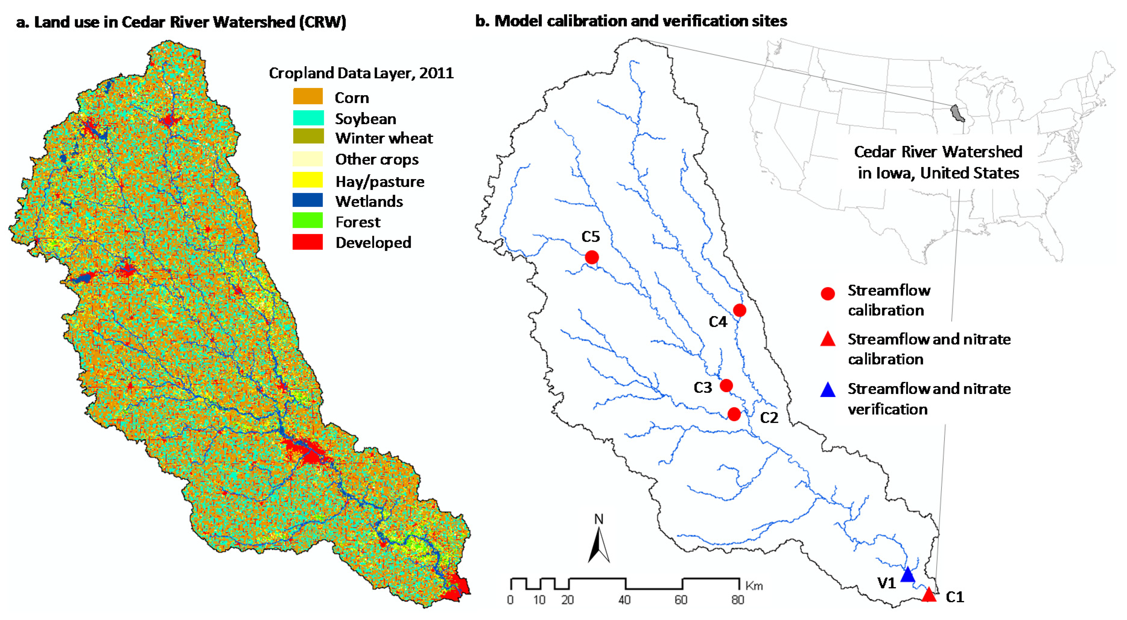
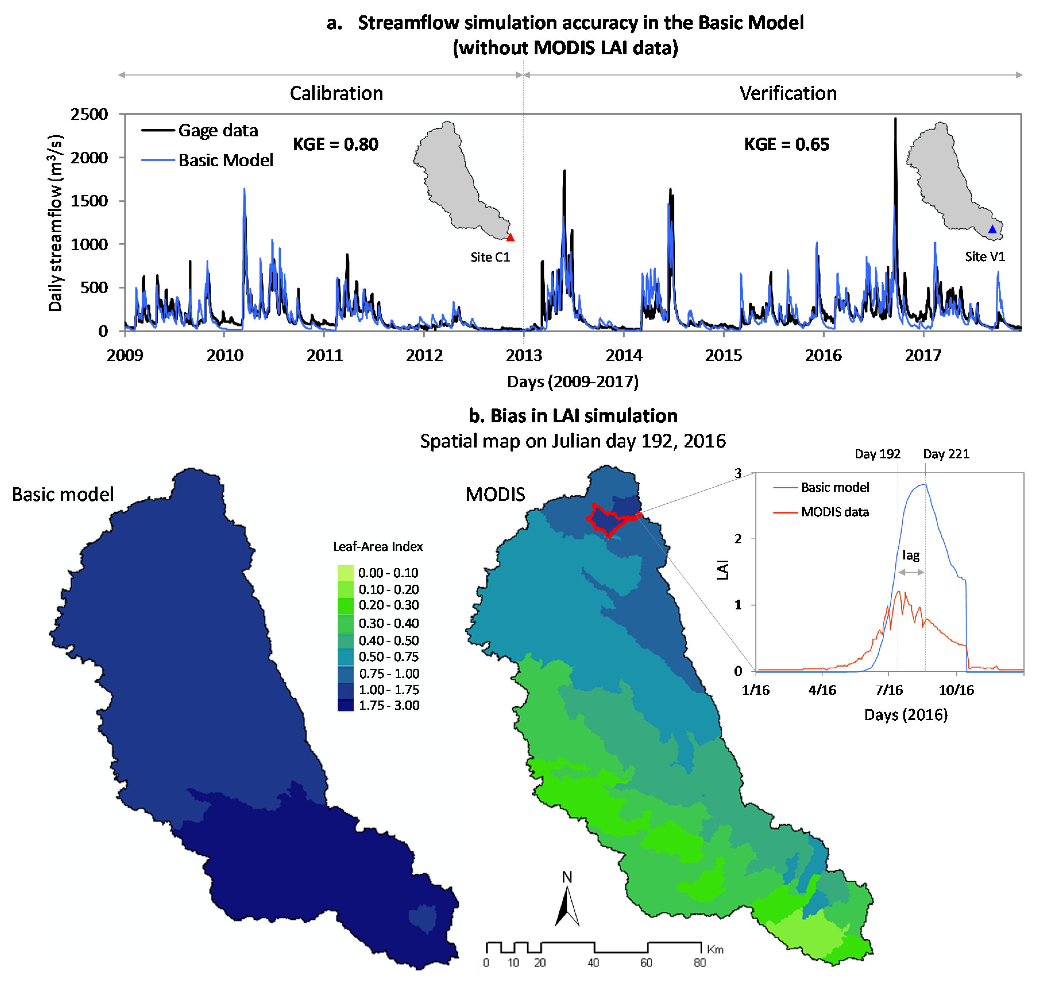
- We assessed the accuracy of daily streamflow simulation for a five-year period (2013–2017) and at a separate gage station not included in the calibration process (for model verification) (Figure 1b).
- We then compared simulated LAI with MODIS data to identify how the calibrated models differ in their respective spatiotemporal representation of vegetation dynamics. For evaluating the spatial accuracy in LAI simulation, we considered specific day(s) in the 2016 crop growing season (June–August). We focused on crop growing season because this is the most active period in terms of vegetation growth and associated water-energy exchanges. We selected 2016 for temporal evaluation because this was a year with average precipitation, hence representative of the watershed’s general hydrologic response.
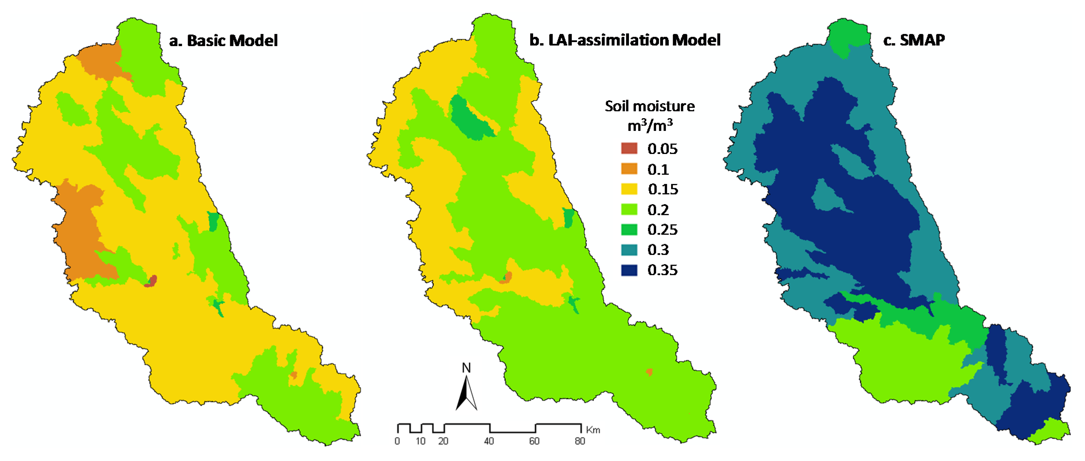
- To further assess improvements in hydrologic simulation, we compared the spatial consistency of soil moisture between model simulations and Soil Moisture Active Passive (SMAP) mission level 4 estimates (Table 1). SMAP mission provides 9-km gridded estimates of rootzone soil moisture, which is a model-assimilated product of remotely sensed surface moisture observations [50]. Briefly, we produced subbasin-level aggregated SMAP data using the same web-based tool and areal averaging procedure described in Section 2.2, took the daily average of rootzone volumetric moisture content over the 2016 crop growing season (June–August), and subsequently generated a watershed soil moisture distribution map to enable spatial comparison with model outputs. We considered the same period for assessment of LAI and soil moisture as it would produce a consistent comparison across two mutually dependent processes. Furthermore, selecting summer months ensured that SMAP data used in our model assessments were not affected by snow cover and frozen soil—the common sources of inaccuracies in remotely sensed soil moisture [59].
- (2)
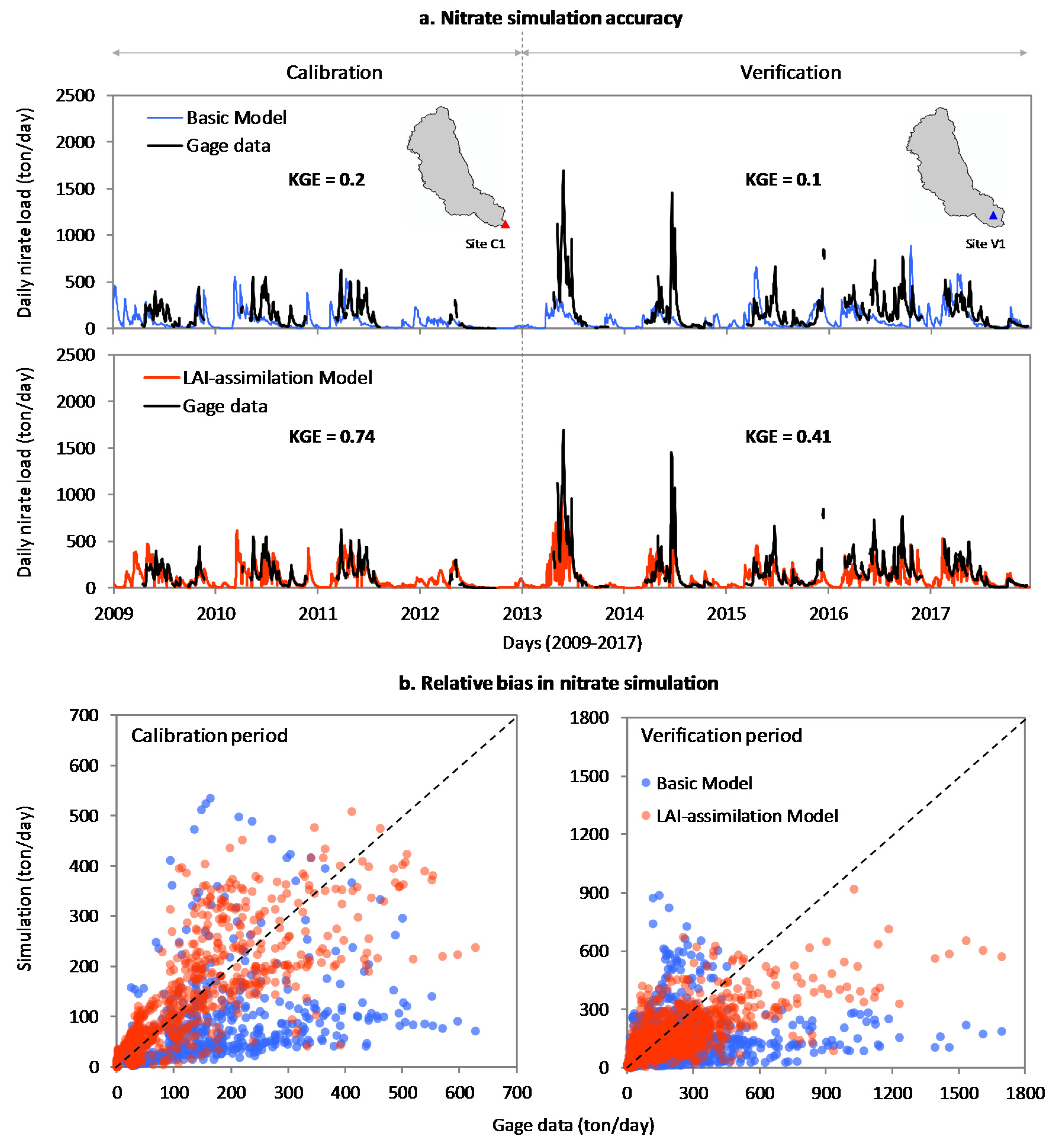
- Assessment of water quality simulation:We assessed the accuracy of daily nitrate load simulation for the same five-year period and at the same location used for streamflow verification (Figure 1b). To the best of our knowledge, this is the first study to verify the effect of LAI data assimilation on water quality simulations and that using long-term daily observations as the reference.
3. Results
3.1. Effect of LAI Data Assimilation on Hydrologic Simulation Accuracy
3.2. Effect of LAI Data Assimilation on Water Quality Simulation Accuracy
4. Discussion
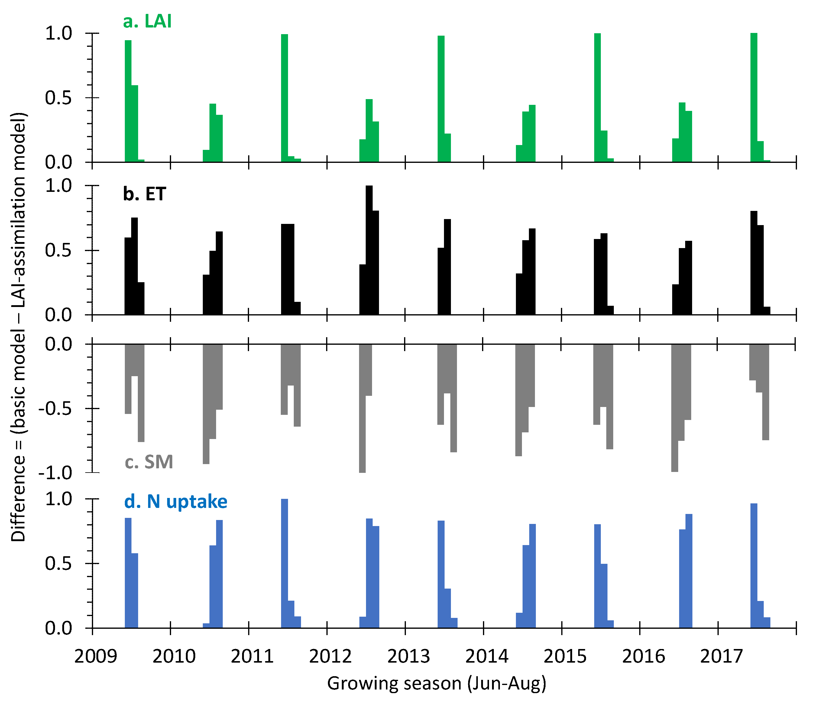
4.1. What Is the Link between Improved LAI Data and Improved Model Predictions?
4.2. Which LAI Datasets Are Appropriate for Watershed-Scale Modeling?
4.3. What Modeling Factors Are Important to Make LAI Data Assimilation Efficient?
5. Summary
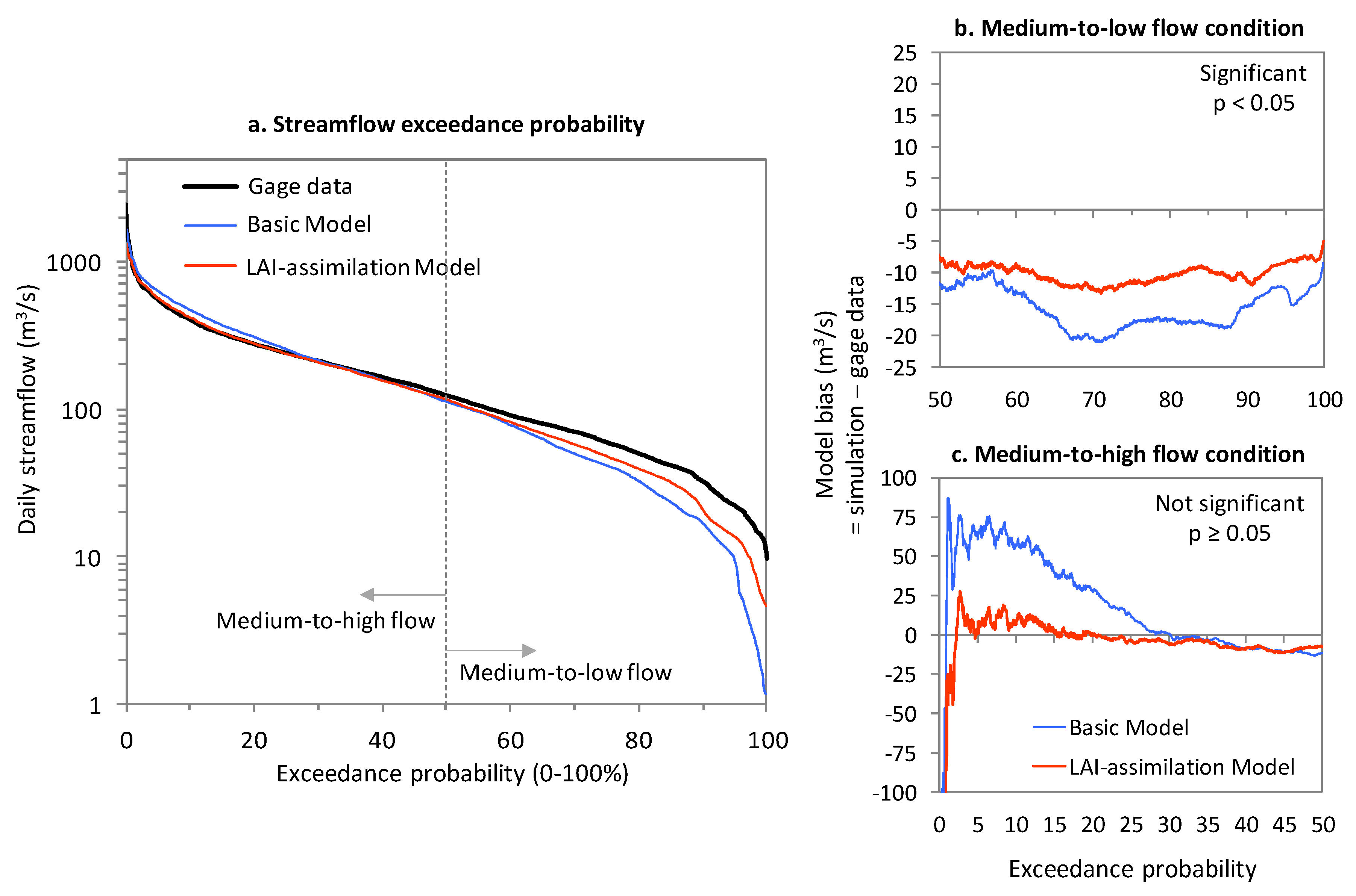
- The basic model gave right answers for wrong reasons, with reasonably good daily streamflow simulation despite a large bias in LAI. The accuracy of daily streamflow simulation improved throughout the nine-year period. However, this improvement was significant during medium-to-low flow conditions.
- The LAI assimilation model adopted a physically realistic water balance by increasing rootzone soil moisture storage, therefore improving the model’s spatial consistency with reference estimates (from the SMAP satellite mission).
- Assimilation of LAI data into our watershed model substantially improved nitrate load simulations, reproducing long-term in-situ observations at a daily timescale. Our study is the first to show such an effect.
Author Contributions
Software Availability
Funding
Conflicts of Interest
Appendix A

| No. | Parameter a | Definition b | Spatial Scale | Initial Range c |
|---|---|---|---|---|
| 1 | ALPHA_BF | Baseflow recession constant (days) | HRU | 0.001–1 |
| 2 | CH_K2 | Channel hydraulic conductivity (mm/h) | Subbasin | 5–100 |
| 3 | CH_N1 | Tributary channel Manning’s n | Subbasin | 0.001–0.15 |
| 4 | CH_N2 | Main channel Manning’s n | Subbasin | 0.001–0.15 |
| 5 | OV_N | Overland Manning’s n | HRU | 0.12 d |
| 6 | CN2 | Curve number (moisture condition II) | HRU | −0.08–0.08 |
| 7 | SURLAG | Surface runoff lag coefficient (days) | Basin | 0.05–10 |
| 8 | EPCO | Plant uptake compensation factor | HRU | 0.01–1 |
| 9 | ESCO | Soil evaporation compensation factor | HRU | 0.01–1 |
| 10 | GW_DELAY | Groundwater delay (days) | HRU | −10–10 |
| 11 | GW_REVAP | Groundwater “revap” coefficient | HRU | 0.01–0.2 |
| 12 | GWQMN | Threshold depth for return flow (mm H2O) | HRU | 0.01–5000 |
| 13 | REVAPMN | Re-evaporation threshold (mm H2O) | HRU | 0.01–500 |
| 14 | RCHRG_DP | Deep aquifer percolation fraction | HRU | 0–1 |
| 15 | SOL_AWC | Available soil water capacity (mm/mm) | HRU | −0.15–0.15 |
| 16 | SOL_K | Soil hydraulic conductivity (mm/h) | HRU | −0.15–0.15 |
| 17 | TIMP | Snow pack temperature lag factor | Basin | 0–1 |
| 18 | SFTMP | Snowfall temperature (°C) | Basin | 0–5 |
| 19 | SMFMN | Min snowmelt factor (mm H2O/°C-day) | Basin | 0–10 |
| 20 | SMFMX | Max snowmelt factor (mm H2O/°C-day) | Basin | 0–10 |
| 21 | SMTMP | Snowmelt base temperature (°C) | Basin | −2–5 |
| No. | Parameter a | Definition b | Spatial Scale | Initial Range c |
|---|---|---|---|---|
| 1 | SPCON | Linear sediment routing factor | Basin | 0.0081 d |
| 2 | SPEXP | Exponent sediment routing factor | Basin | 1 d |
| 4 | CH_COV1 | Channel erodibility factor | Subbasin | 0.22 d |
| 3 | CH_COV2 | Channel cover factor | Subbasin | 0.1 d |
| 5 | PHOSKD | Phosphorus soil partitioning coefficient | Basin | 167 d |
| 6 | PPERCO | Phosphorus percolation coefficient | Basin | 11.2 d |
| 7 | SOL_ORGP | Initial organic P conc. in soil layer (mg P/kg) | HRU | 10 d |
| 8 | SOL_ORGN | Initial organic N conc. in soil layer (mg N/kg) | HRU | 1–50 |
| 9 | SOL_NO3 | Initial NO3 concentration in soil layer (mg N/kg) | HRU | 1–50 |
| 10 | SOL_CBN | Organic carbon content in soil layer (% weight) | HRU | 0.05–10 |
| 11 | BIOMIX | Biological mixing efficiency | HRU | 0.001–1 |
| 12 | CDN | Denitrification exponential rate | Basin | 0.001–3 |
| 13 | CMN | Mineralization rate of active N and P | Basin | 0.001–0.003 |
| 14 | HLIFE_NGW | Half-life of nitrogen in ground water (days) | Basin | 0–500 |
| 15 | NPERCO | Nitrate percolation coefficient | Basin | 0.001–1 |
| 16 | SDNCO | Denitrification threshold water content | Basin | 0.001–1.1 |
| 17 | ANION_EXCL | Fraction of porosity to exclude anions | Basin | 0.01–1 |
| 18 | BC1 | Biological oxidation rate (NH3) (day−1) | Basin | 0.1–1 |
| 19 | BC2 | Biological oxidation rate (NO2-NO3) (day−1) | Basin | 0.2–2 |
| 20 | BC3 | Biological oxidation rate (organic N-NH3) (day−1) | Basin | 0.02–0.4 |
| 21 | RS4 | Organic N settling rate in the channel (day−1) | Subbasin | 0.001–0.1 |
References
- Beven, K.J. Towards a Coherent Philosophy for Environmental Modelling. Royal Soc. 2002, 458, 2465–2484. [Google Scholar] [CrossRef]
- Ruddell, B.L.; Drewry, D.T.; Nearing, G.S. Information Theory for Model Diagnostics: Structural Error is Indicated by Trade-Off Between Functional and Predictive Performance. Water Resour. Res. 2019, 55, 6534–6554. [Google Scholar] [CrossRef]
- Golden, H.E.; Rajib, A.; Lane, C.R.; Christensen, J.R.; Wu, Q.; Mengistu, S.G. Non-floodplain Wetlands Affect Watershed Nutrient Dynamics: A Critical Review. Environ. Sci. Technol. 2019, 53, 7203–7214. [Google Scholar] [CrossRef] [PubMed]
- Rajib, A.; Ahiablame, L.; Paul, M. Modeling the effects of future land use change on water quality under multiple scenarios: A case study of low-input agriculture with hay/pasture production. Sustain. Water Qual. Ecol. 2016, 8, 50–66. [Google Scholar] [CrossRef]
- Du, L.; Rajib, A.; Merwade, V. Large scale spatially explicit modeling of blue and green water dynamics in a temperate mid-latitude basin. J. Hydrol. 2018, 562, 84–102. [Google Scholar] [CrossRef]
- Kunnath-Poovakka, A.; Ryu, D.; Renzullo, L.J.; George, B. Remotely sensed ET for streamflow modelling in catchments with contrasting flow characteristics: An attempt to improve efficiency. Stoch. Environ. Res. Risk Assess. 2018, 32, 1973–1992. [Google Scholar] [CrossRef]
- Rajib, A.; Merwade, V.; Yu, Z. Rationale and Efficacy of Assimilating Remotely Sensed Potential Evapotranspiration for Reduced Uncertainty of Hydrologic Models. Water Resour. Res. 2018, 54, 4615–4637. [Google Scholar] [CrossRef]
- Rajib, A.; Evenson, G.R.; Golden, H.E.; Lane, C.R. Hydrologic model predictability improves with spatially explicit calibration using remotely sensed evapotranspiration and biophysical parameters. J. Hydrol. 2018, 567, 668–683. [Google Scholar] [CrossRef]
- Rajib, A.; Merwade, V.; Yu, Z. Multi-objective calibration of a hydrologic model using spatially distributed remotely sensed/in-situ soil moisture. J. Hydrol. 2016, 536, 192–207. [Google Scholar] [CrossRef]
- Brocca, L.; Moramarco, T.; Melone, F.; Wagner, W.; Hasenauer, S.; Hahn, S. Assimilation of Surface- and Root-Zone ASCAT Soil Moisture Products into Rainfall Runoff Modeling. IEEE Trans. Geosci. Remote Sens. 2011, 50, 2542–2555. [Google Scholar] [CrossRef]
- Fang, H.; Liang, S. Leaf area index models. In Encyclopedia of Ecology; Fath, D., Ed.; Academic Press: Oxford, UK, 2008; pp. 2139–2148. [Google Scholar] [CrossRef]
- Demarty, J.; Chevallier, F.; Viovy, N.; Friend, A.D.; Piao, S.; Ciais, P. Assimilation of global MODIS leaf area index retrievals within a terrestrial biosphere model. Geophys. Res. Lett. 2007, 34, 1–6. [Google Scholar] [CrossRef]
- Nair, S.S.; King, K.; Witter, J.D.; Sohngen, B.L.; Fausey, N.R. Importance of Crop Yield in Calibrating Watershed Water Quality Simulation Tools1. JAWRA J. Am. Water Resour. Assoc. 2011, 47, 1285–1297. [Google Scholar] [CrossRef]
- Fang, H.; Baret, F.; Plummer, S.; Schaepman-Strub, G. An Overview of Global Leaf Area Index (LAI): Methods, Products, Validation, and Applications. Rev. Geophys. 2019, 57, 739–799. [Google Scholar] [CrossRef]
- Qu, Y.; Zhuang, Q. Modeling leaf area index in North America using a process-based terrestrial ecosystem model. Ecosphere 2018, 9, e02046. [Google Scholar] [CrossRef]
- Ling, X.; Fu, C.; Guo, W.; Yang, Z.-L. Assimilation of Remotely Sensed LAI into CLM4CN Using DART. J. Adv. Model. Earth Syst. 2019, 11, 2768–2786. [Google Scholar] [CrossRef]
- Mokhtari, A.; Noory, H.; Vazifedoust, M. Improving crop yield estimation by assimilating LAI and inputting satellite-based surface incoming solar radiation into SWAP model. Agric. For. Meteorol. 2018, 2018, 159–170. [Google Scholar] [CrossRef]
- Ines, A.V.M.; Das, N.N.; Hansen, J.; Njoku, E.G. Assimilation of remotely sensed soil moisture and vegetation with a crop simulation model for maize yield prediction. Remote Sens. Environ. 2013, 138, 149–164. [Google Scholar] [CrossRef]
- Muñoz-Sabater, J.; Rüdiger, C.; Calvet, J.-C.; Fritz, N.; Jarlan, L.; Kerr, Y. Joint assimilation of surface soil moisture and LAI observations into a land surface model. Agric. For. Meteorol. 2008, 148, 1362–1373. [Google Scholar] [CrossRef]
- Barbu, A.L.; Calvet, J.-C.; Mahfouf, J.-F.; Albergel, C.; Lafont, S. Assimilation of Soil Wetness Index and Leaf Area Index into the ISBA-A-gs land surface model: Grassland case study. Biogeosciences 2011, 8, 1971–1986. [Google Scholar] [CrossRef]
- Neitsch, S.; Arnold, J.; Kiniry, J.; Williams, J. Soil & Water Assessment Tool Theoretical Documentation Version 2009; Texas Water Resources Institute Technical Report No. 406; Texas A&M University System: College Station, TX, USA, 2011; Available online: https://swat.tamu.edu/media/99192/swat2009-theory.pdf (accessed on 3 July 2020).
- Strauch, M.; Volk, M. SWAT plant growth modification for improved modeling of perennial vegetation in the tropics. Ecol. Model. 2013, 269, 98–112. [Google Scholar] [CrossRef]
- Alemayehu, T.; Van Griensven, A.; Woldegiorgis, B.T.; Bauwens, W. An improved SWAT vegetation growth module and its evaluation for four tropical ecosystems. Hydrol. Earth Syst. Sci. 2017, 21, 4449–4467. [Google Scholar] [CrossRef]
- Ford, T.W.; Quiring, S.M. Influence of MODIS-Derived Dynamic Vegetation on VIC-Simulated Soil Moisture in Oklahoma. J. Hydrometeorol. 2013, 14, 1910–1921. [Google Scholar] [CrossRef]
- Parr, D.; Wang, G.; Bjerklie, D. Integrating Remote Sensing Data on Evapotranspiration and Leaf Area Index with Hydrological Modeling: Impacts on Model Performance and Future Predictions. J. Hydrometeorol. 2015, 16, 2086–2100. [Google Scholar] [CrossRef]
- US Army Corps of Engineers. Hydrologic Modeling System User’s Manual Version 4.3; US Army Hydrologic Engineering Centre: Davis, CA, USA, 2018. Available online: https://www.hec.usace.army.mil/software/hec-hms/documentation/HEC-HMS_Users_Manual_4.3.pdf (accessed on 29 June 2020).
- Albergel, C.; Munier, S.; Leroux, D.J.; Dewaele, H.; Fairbairn, D.; Barbu, A.L.; Gelati, E.; Dorigo, W.; Faroux, S.; Meurey, C.; et al. Sequential assimilation of satellite-derived vegetation and soil moisture products using SURFEX_v8.0: LDAS-Monde assessment over the Euro-Mediterranean area. Geosci. Model Dev. 2017, 10, 3889–3912. [Google Scholar] [CrossRef]
- Kumar, S.V.; Mocko, D.M.; Wang, S.; Peters-Lidard, C.D.; Borak, J. Assimilation of Remotely Sensed Leaf Area Index into the Noah-MP Land Surface Model: Impacts on Water and Carbon Fluxes and States over the Continental United States. J. Hydrometeorol. 2019, 20, 1359–1377. [Google Scholar] [CrossRef]
- Zhang, X.; Maggioni, V.; Rahman, A.; Houser, P.; Xue, Y.; Sauer, T.; Kumar, S.; Mocko, D. The Influence of Assimilating Leaf Area Index in a Land Surface Model on Global Water Fluxes and Storages. Hydrol. Earth Syst. Sci. Discuss. 2019, 1–28. [Google Scholar] [CrossRef]
- Ma, T.; Duan, Z.; Li, R.; Song, X. Enhancing SWAT with remotely sensed LAI for improved modelling of ecohydrological process in subtropics. J. Hydrol. 2019, 570, 802–815. [Google Scholar] [CrossRef]
- Myneni, R.; Knyazikhin, Y.; Park, T. MCD15A3H MODIS/Terra+Aqua Leaf Area Index/FPAR 4-Day L4 Global 500m SIN Grid V006. 2015. Available online: https://lpdaac.usgs.gov/products/mcd15a3hv006/ (accessed on 29 June 2020).
- Mallakpour, I.; Villarini, G. The changing nature of flooding across the central United States. Nat. Clim. Chang. 2015, 5, 250–254. [Google Scholar] [CrossRef]
- Easterling, D.; Arnold, J.; Knutson, T.; Kunkel, K.; LeGrande, A.; Leung, L.; Vose, R.; Waliser, D.; Wehner, M.F. Precipitation. In Climate Science Special Report: Fourth National Climate Assessment, Volume I; Wuebbles, D.J., Fahey, D.W., Hibbard, K.A., Eds.; U.S. Global Change Research Program: Washington, DC, USA, 2017; pp. 207–230. Available online: https://science2017.globalchange.gov/chapter/7/ (accessed on 29 June 2020).
- Paul, M.; Rajib, A.; Ahiablame, L. Spatial and Temporal Evaluation of Hydrological Response to Climate and Land Use Change in Three South Dakota Watersheds. JAWRA J. Am. Water Resour. Assoc. 2016, 53, 69–88. [Google Scholar] [CrossRef]
- Wu, Y.; Liu, S.; Sohl, T.; Young, C.J. Projecting the land cover change and its environmental impacts in the Cedar River Basin in the Midwestern United States. Environ. Res. Lett. 2013, 8, 024025. [Google Scholar] [CrossRef]
- Rajib, A.; Merwade, V. Hydrologic response to future land use change in the Upper Mississippi River Basin by the end of 21st century. Hydrol. Process. 2017, 31, 3645–3661. [Google Scholar] [CrossRef]
- Hutchinson, K.; Christiansen, D. Use of the Soil and Water Assessment Tool (SWAT) for Simulating Hydrology and Water Quality in the Cedar River Basin, Iowa, 2000–10; U.S. Geological Survey Scientific Investigations Report 2013–5002; U.S. Geological Survey: Iowa City, IA, USA, 2013. Available online: https://pubs.usgs.gov/sir/2013/5002/ (accessed on 29 June 2020).
- Wu, Y.; Liu, S. Impacts of biofuels production alternatives on water quantity and quality in the Iowa River Basin. Biomass- Bioenergy 2012, 36, 182–191. [Google Scholar] [CrossRef]
- Le, L. Modeling Stream Discharge and Nitrate Loading in the Iowa-Cedar River Basin under Climate and Land Use Change. Ph.D. Thesis, University of Iowa, Iowa City, IA, USA, 2015. Available online: https://ir.uiowa.edu/etd/1872/ (accessed on 29 June 2020).
- Schuol, J.; Abbaspour, K.C.; Yang, H.; Srinivasan, R.; Zehnder, A.J. Modeling blue and green water availability in Africa. Water Resour. Res. 2008, 44, 1–18. [Google Scholar] [CrossRef]
- Schierhorn, F.; Faramarzi, M.; Prishchepov, A.V.; Koch, F.J.; Müller, D. Quantifying yield gaps in wheat production in Russia. Environ. Res. Lett. 2014, 9, 084017. [Google Scholar] [CrossRef]
- Rajib, A.; Golden, H.E.; Lane, C.R.; Wu, Q. Surface depression and wetland water storage improves major river basin hydrologic predictions. Water Resour. Res. 2020. [Google Scholar] [CrossRef]
- Rajib, A.; Liu, Z.; Merwade, V.; Tavakoly, A.A.; Follum, M.L. Towards a large-scale locally relevant flood inundation modeling framework using SWAT and LISFLOOD-FP. J. Hydrol. 2020, 581, 124406. [Google Scholar] [CrossRef]
- Ilampooranan, I.; Van Meter, K.J.; Basu, N.B. A Race Against Time: Modeling Time Lags in Watershed Response. Water Resour. Res. 2019, 55, 3941–3959. [Google Scholar] [CrossRef]
- Faramarzi, M.; Abbaspour, K.C.; Adamowicz, W.L.V.; Lu, W.; Fennell, J.; Zehnder, A.J.; Goss, G.G. Uncertainty based assessment of dynamic freshwater scarcity in semi-arid watersheds of Alberta, Canada. J. Hydrol. Reg. Stud. 2017, 9, 48–68. [Google Scholar] [CrossRef]
- US Geological Survey National Elevation Dataset (USGS-NED). National Map Viewer. Available online: http://viewer.nationalmap.gov/viewer/ (accessed on 10 October 2018).
- National Agricultural Statistics Service Cropland Data Layer (NASS-CDL), US Department of Agriculture CropScape. Available online: https://nassgeodata.gmu.edu/CropScape/ (accessed on 10 October 2018).
- Natural Resources Conservation Service. U.S. Department of Agriculture Soil Survey Staff. Available online: https://websoilsurvey.nrcs.usda.gov/ (accessed on 10 October 2018).
- Thornton, P.E.; Thornton, M.M.; Mayer, B.W.; Wei, Y.; Devarakonda, R.; Vose, R.S.; Cook, R.B. DAYMET: Daily Surface Weather Data on a 1-km Grid for North America, Version 3; ORNL DAAC: Oak Ridge, TN, USA, 2018. [Google Scholar] [CrossRef]
- Reichle, R.; De Lannoy, G.; Koster, R.D.; Crow, W.; Kimball, J.; Liu, Q. SMAP L4 Global 3-Hourly 9 km EASE-Grid Surface and Root Zone Soil Moisture Geophysical Data, Version 4; NASA National Snow and Ice Data Center Distributed Active Archive Center: Boulder, CO, USA, 2018. [CrossRef]
- Rajib, A.; Merwade, V.; Zhao, L.; Shin, J.; Smith, J.; Song, C. HydroGlobe Tool. 2018. Available online: https://mygeohub.org/resources/hydroglobetool (accessed on 9 June 2020).
- Meng, C.; Zhang, C.; Tang, R. Variational Estimation of Land–Atmosphere Heat Fluxes and Land Surface Parameters Using MODIS Remote Sensing Data. J. Hydrometeorol. 2013, 14, 608–621. [Google Scholar] [CrossRef]
- Kalkhoff, S.J. Transport of nitrogen and phosphorus in the Cedar River Basin, Iowa and Minnesota, 2000–2015. US Geol. Surv. 2018, 44. [Google Scholar] [CrossRef]
- Jones, C.; Davis, C.A.; Drake, C.W.; Schilling, K.E.; Debionne, S.H.; Gilles, D.W.; Demir, I.; Weber, L. Iowa Statewide Stream Nitrate Load Calculated Using In Situ Sensor Network. JAWRA J. Am. Water Resour. Assoc. 2017, 54, 471–486. [Google Scholar] [CrossRef]
- Holder, A.J.; Rowe, R.; McNamara, N.P.; Donnison, I.S.; McCalmont, J. Soil & Water Assessment Tool (SWAT) simulated hydrological impacts of land use change from temperate grassland to energy crops: A case study in western UK. GCB Bioenergy 2019, 11, 1298–1317. [Google Scholar] [CrossRef]
- Lin, P.; Rajib, A.; Yang, Z.-L.; Somos-Valenzuela, M.; Merwade, V.; Maidment, D.R.; Wang, Y.; Chen, L. Spatiotemporal Evaluation of Simulated Evapotranspiration and Streamflow over Texas Using the WRF-Hydro-RAPID Modeling Framework. JAWRA J. Am. Water Resour. Assoc. 2017, 54, 40–54. [Google Scholar] [CrossRef]
- Abbaspour, K.C. SWAT-CUP 2012: SWAT Calibration and Uncertainty Programs—A User Manual; Swiss Federal Institute of Aquatic Science and Technology: Dübendorf, Switzerland, 2015; Available online: http://swat.tamu.edu/media/114860/usermanual_swatcup.pdf (accessed on 9 June 2019).
- Gupta, H.; Kling, H.; Yilmaz, K.K.; Martinez, G.F. Decomposition of the mean squared error and NSE performance criteria: Implications for improving hydrological modelling. J. Hydrol. 2009, 377, 80–91. [Google Scholar] [CrossRef]
- Reichle, R.H.; De Lannoy, G.J.; Liu, Q.; Ardizzone, J.V.; Colliander, A.; Conaty, A.; Crow, W.T.; Jackson, T.J.; Jones, L.A.; Kimball, J.S.; et al. Assessment of the SMAP Level-4 Surface and Root-Zone Soil Moisture Product Using In Situ Measurements. J. Hydrometeorol. 2017, 18, 2621–2645. [Google Scholar] [CrossRef]
- Efstratiadis, A.; Koutsoyiannis, D. One decade of multi-objective calibration approaches in hydrological modelling: A review. Hydrol. Sci. J. 2010, 55, 58–78. [Google Scholar] [CrossRef]
- Vermote, E. NOAA Climate Data Record (CDR) of AVHRR Leaf Area Index (LAI) and Fraction of Absorbed Photosynthetically Active Radiation (FAPAR), Version 5; NOAA National Centers for Environmental Information: Asheville, NC, USA, 2019. [CrossRef]
- Claverie, M.; Matthews, J.L.; Vermote, E.F.; Justice, C.O. A 30+ Year AVHRR LAI and FAPAR Climate Data Record: Algorithm Description and Validation. Remote Sens. 2016, 8, 263. [Google Scholar] [CrossRef]
- Zhu, Z.; Bi, J.; Pan, Y.; Ganguly, S.; Anav, A.; Xu, L.; Samanta, A.; Piao, S.; Nemani, R.; Myneni, R. Global Data Sets of Vegetation Leaf Area Index (LAI)3g and Fraction of Photosynthetically Active Radiation (FPAR)3g Derived from Global Inventory Modeling and Mapping Studies (GIMMS) Normalized Difference Vegetation Index (NDVI3g) for the Period 1981 to 2011. Remote Sens. 2013, 5, 927–948. [Google Scholar] [CrossRef]
- Xiao, Z.; Liang, S.; Wang, J.; Chen, P.; Yin, X.; Zhang, L.; Song, J. Use of General Regression Neural Networks for Generating the GLASS Leaf Area Index Product from Time-Series MODIS Surface Reflectance. IEEE Trans. Geosci. Remote Sens. 2013, 52, 209–223. [Google Scholar] [CrossRef]
- Yan, K.; Park, T.; Yan, G.; Chen, C.; Yang, B.; Liu, Z.; Nemani, R.; Knyazikhin, Y.; Myneni, R. Evaluation of MODIS LAI/FPAR Product Collection 6. Part 1: Consistency and Improvements. Remote Sens. 2016, 8, 359. [Google Scholar] [CrossRef]
- Yan, K.; Park, T.; Yan, G.; Liu, Z.; Yang, B.; Chen, C.; Nemani, R.; Knyazikhin, Y.; Myneni, R. Evaluation of MODIS LAI/FPAR Product Collection 6. Part 2: Validation and Intercomparison. Remote Sens. 2016, 8, 460. [Google Scholar] [CrossRef]
- Yang, W.; Tan, B.; Huang, D.; Rautiainen, M.; Shabanov, N.; Wang, Y.; Privette, J.; Huemmrich, K.; Fensholt, R.; Sandholt, I.; et al. MODIS leaf area index products: From validation to algorithm improvement. IEEE Trans. Geosci. Remote Sens. 2006, 44, 1885–1898. [Google Scholar] [CrossRef]
- Jiang, C.; Ryu, Y.; Fang, H.; Myneni, R.; Claverie, M.; Zhu, Z. Inconsistencies of interannual variability and trends in long-term satellite leaf area index products. Glob. Chang. Biol. 2017, 23, 4133–4146. [Google Scholar] [CrossRef] [PubMed]
- Kumar, S.; Peters-Lidard, C.; Tian, Y.; Houser, P.; Geiger, J.; Olden, S.; Lighty, L.; Eastman, J.; Doty, B.; Dirmeyeri, P.A.; et al. Land information system: An interoperable framework for high resolution land surface modeling. Environ. Model. Softw. 2006, 21, 1402–1415. [Google Scholar] [CrossRef]


| Item | Description |
|---|---|
| Topography | 30-m National Elevation Dataset [46] |
| Land use | 30-m 2011 Cropland Data Layer [47] |
| Soil texture | 1:250,000 State Soil Geographic (STATSGO) dataset [48] |
| Slope | Five slope classes: 0–2%, 2–4%, 4–6%, 6–8%, >8% [3,39] |
| Subsurface drainage | Tile drains were assigned on low slope (<2%) with row crops and poorly drained soils (hydrologic soil group D) [3,37,38] |
| Agricultural management operations | (a) Timing of plantation and harvest; (b) timing, type, rate, and place of fertilizer applications; (c) corn–soybean annual rotation [3,37] |
| Precipitation | Total daily precipitation from 1-km gridded DAYMET product [49] |
| Energy-related weather forcing | Minimum and maximum daily temperature from 1-km gridded DAYMET product [49]; solar radiation, wind speed and relative humidity from the historical weather generator within the SWAT source-code [21]; potential evapotranspiration (PET) estimated with built-in Penman-Monteith equation [21] |
| Streamflow and nitrate data | Six U.S. Geological Survey (USGS) gage stations; five for model calibration and one for model verification (Figure 1b) |
| Rootzone (100 cm) soil moisture data | Soil Moisture Active Passive (SMAP) mission 3-hourly L4 global 9-km rootzone soil moisture; used for model verification [50] |
| LAI data | MODIS MCD15A3H LAI/FPAR four-day L4 global 500 m v006 [31]; assimilated in the model replacing the model’s default LAI values |
| Location a | Basic Model | LAI-Assimilation Model | |
|---|---|---|---|
| Calibration | C1b | 0.80 | 0.86 |
| C2 | 0.84 | 0.85 | |
| C3 | 0.87 | 0.87 | |
| C4 | 0.50 | 0.51 | |
| C5 | 0.55 | 0.64 | |
| Verification | V1 | 0.65 | 0.72 |
© 2020 by the authors. Licensee MDPI, Basel, Switzerland. This article is an open access article distributed under the terms and conditions of the Creative Commons Attribution (CC BY) license (http://creativecommons.org/licenses/by/4.0/).
Share and Cite
Rajib, A.; Kim, I.L.; Golden, H.E.; Lane, C.R.; Kumar, S.V.; Yu, Z.; Jeyalakshmi, S. Watershed Modeling with Remotely Sensed Big Data: MODIS Leaf Area Index Improves Hydrology and Water Quality Predictions. Remote Sens. 2020, 12, 2148. https://doi.org/10.3390/rs12132148
Rajib A, Kim IL, Golden HE, Lane CR, Kumar SV, Yu Z, Jeyalakshmi S. Watershed Modeling with Remotely Sensed Big Data: MODIS Leaf Area Index Improves Hydrology and Water Quality Predictions. Remote Sensing. 2020; 12(13):2148. https://doi.org/10.3390/rs12132148
Chicago/Turabian StyleRajib, Adnan, I Luk Kim, Heather E. Golden, Charles R. Lane, Sujay V. Kumar, Zhiqiang Yu, and Saranya Jeyalakshmi. 2020. "Watershed Modeling with Remotely Sensed Big Data: MODIS Leaf Area Index Improves Hydrology and Water Quality Predictions" Remote Sensing 12, no. 13: 2148. https://doi.org/10.3390/rs12132148
APA StyleRajib, A., Kim, I. L., Golden, H. E., Lane, C. R., Kumar, S. V., Yu, Z., & Jeyalakshmi, S. (2020). Watershed Modeling with Remotely Sensed Big Data: MODIS Leaf Area Index Improves Hydrology and Water Quality Predictions. Remote Sensing, 12(13), 2148. https://doi.org/10.3390/rs12132148