Abstract
The total suspended matter (TSM) variability plays a crucial role in a lake’s ecological functioning and its biogeochemical cycle. Sentinel-2A MultiSpectral Instrument (MSI) and Landsat 8 Operational Land Instrument (OLI) data offer unique opportunities for investigating certain in-water constituents (e.g., TSM and chlorophyll-a) owing to their spatial resolution (10–60 m). In this framework, we assessed the potential of MSI–OLI combined data in characterizing the multi-temporal (2014–2018) TSM variability in Pertusillo Lake (Basilicata region, Southern Italy). We developed and validated a customized MSI-based TSM model (R2 = 0.81) by exploiting ground measurements acquired during specific measurement campaigns. The model was then exported as OLI data through an intercalibration procedure (R2 = 0.87), allowing for the generation of a TSM multi-temporal MSI–OLI merged dataset. The analysis of the derived multi-year TSM monthly maps showed the influence of hydrological factors on the TSM seasonal dynamics over two sub-regions of the lake, the west and east areas. The western side is more influenced by inflowing rivers and water level fluctuations, the effects of which tend to longitudinally decrease, leading to less sediment within the eastern sub-area. The achieved results can be exploited by regional authorities for better management of inland water quality and monitoring systems.
1. Introduction
Inland freshwater bodies are key providers of services to local communities, being crucial sources of drinking water and major hubs for recreational activities [1]. However, like many other ecosystems, lakes are affected by increasing environmental pressures due to co-occurring stressors such as climate change, contamination of organic and inorganic substances, and anthropogenic influences, which threaten their ecological functions [2,3]. For this reason, European legislation such as the Marine Strategy Framework Directive (MSFD, 2008/56/EC) and Water Framework Directive (WFD, 2000/60/EC and amendments) requires member states to assess the ecological status of water bodies based on different quality indicators, such as water transparency [4]. This parameter is strongly linked to the amount of suspended matter (i.e., total suspended matter—TSM) outflowing into lakes from terrestrial environments via river discharge [5]. TSM is mainly characterized by non-algal organic detritus and mineral sediments, and it is a key bio-optical constituent in lakes’ ecological function and biogeochemical cycle [6]. Sediments can directly reduce light penetration, inhibiting phytoplankton productivity as well as affecting nutrient dynamics [7] and the transport of micropollutants, heavy metals, and other materials [8]. TSM field measurements are time-consuming, expensive, and site-dependent, and therefore it is not always possible to measure TSM dynamics in the spatiotemporal domain [9]. Ocean-color (OC) remote sensing can be useful for complementing in situ TSM measurements, since it can ensure routine synoptic views in a cost-effective way [10,11,12]. OC sensors can provide information on bio-optical in-water constituents such as TSM, acquiring measurements of water leaving radiance in the visible (VIS) and near-infrared (NIR) spectral regions [13]. For instance, Moderate-Resolution Imaging Spectroradiometer (MODIS) and Medium-Resolution Imaging Spectrometer (MERIS) technologies have been widely employed in numerous studies aimed at analyzing the TSM distribution in inland and coastal turbid waters [14,15,16]. Furthermore, these OC sensors have been used to investigate water quality indicators or to develop TSM estimation models, especially for large lakes such as Lake Balaton [17], Lake Taihu [11], the Great Lakes [18], and Lake Geneva [19]. However, the above-mentioned sensors, which are mainly designed for marine research (i.e., open and coastal waters), have coarse spatial resolutions, making them unsuitable for remote-sensing applications over most lakes and reservoirs [20]. The new generation of sensors such as the MultiSpectral Instrument (MSI) on Sentinel-2A/B(S2A/B) and the Operational Land Imager (OLI) on Landsat 8 (L8) allow these limitations to be overcome, offering unprecedented opportunities for lake remote sensing, although they are designed mostly for land applications [21].
Recent publications have corroborated the capability of MSI-S2A and OLI-L8 (hereinafter MSI and OLI, respectively) data for water resource monitoring, especially for inland waters or small lakes. For instance, Gernez et al. [22] analyzed the MSI-derived TSM distribution over an oyster farm under different tidal conditions. Liu et al. [23] assessed the applicability of MSI-S2A data for TSM retrieval in Poyang Lake, and Toming et al. [24] tested the suitability of the same kind of data for mapping several indicators of water quality in at least nine small lakes (≤3 km2). Referring also to OLI data, Eder et al. [25] employed these data to investigate mineral-rich suspended matter in glacial lakes, and Giardino et al. [10] evaluated their value for estimating in-water bio-optical constituents in Garda Lake (Italy). Within the studies performed using both MSI and OLI data, Manzo et al. [26] carried out a sensitivity analysis of the contributions of optically active matter types in the spectral bands of Landsat-8 and Sentinel-2 for Italian lakes, while Lavrova et al. [27] used the above-mentioned data to study fine-scale hydrodynamic processes close to river plumes in the Black Sea. Furthermore, Pahlevan et al. [28] demonstrated how MSI–OLI combined data open new opportunities for monitoring coastal and inland waters at rates that have never been possible before, owing to their improved temporal coverage at 10–60 m spatial resolution. The consequent increase in the average revisit interval time, as well as in the number of cloud-free images, can ensure better capture of the dynamics of inland waters [28]. Most of the above-mentioned studies were performed at regional/local scale based on site-specific radiometric and bio-optical measurements, thus allowing for the development and implementation of customized TSM models, especially for ecologically relevant reservoirs or poorly studied lakes.
Pertusillo Lake (hereinafter PL) (Basilicata region, Southern Italy) is one of the least investigated reservoirs within the Italian Peninsula and has never been studied using satellite data, although the increase of human activities in the high Agri Valley enhanced its environmental relevance. The proximity to wastewater-treatment plants, landfills, farms, plastics, and other industrial activities is threatening the environmental equilibrium of the freshwater reservoir [29]. Among these activities, it is worth mentioning the exploitation, in the same area, of the largest onshore oil field in Western Europe characterized by crude oil extractions from 26 wells to produce about 104 × 103 barrels∙day−1 (nominal capacity of treatment) [30]. The heavy metals or other micro-pollutants released by these industrial activities may tend to accumulate both in soils [31] and in lake ecosystems, in suspended form via runoff, thus reducing the water’s transparency [32]. In this scenario, the characterization of the TSM variability represents a relevant environmental challenge to be addressed for this freshwater reservoir, which lacks continuous in situ monitoring networks and, thus, may benefit from the integration of satellite data. Assuming that several inland water bodies are characterized by similar conditions, it is worth defining a common integrated approach that will be useful for their investigation.
In this context, this work describes the development of a multi-source methodological approach (i.e., in situ data collection, modeling, and satellite-data processing) to assess the TSM multi-temporal variability in a freshwater lake by exploiting the combined use of MSI and OLI data. To achieve this purpose, the study aimed to (1) develop a PL-tuned version of MSI TSM model by exploiting a dataset of radiometric and TSM in situ measurements; (2) export the above-mentioned TSM model to OLI data through an intercalibration procedure; and (3) generate TSM maps based on a multi-year (2014–2018) MSI–OLI combined dataset to assess the TSM variability over PL. The implementation of such an integrated and sustainable approach could provide a useful basis for further studies focused on water-quality monitoring of inland waters.
2. Materials and Methods
2.1. Study Area
PL is a human-made freshwater reservoir (Figure 1b) located in the high Agri Valley (Basilicata region, Southern Italy) within a typical Mediterranean agro-forestry system [33]. PL was formed during the 1957–1963 years through the construction of a dam wall across the Agri River, in the upper part of this valley, and it falls within the municipal boundaries of Grumento Nova, Montemurro, and Spinoso (Figure 1c).
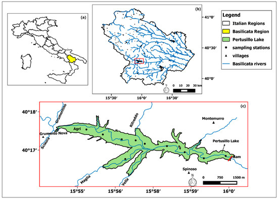
Figure 1.
(a) Location (highlighted in yellow) of the Basilicata region within the Italian peninsula; (b) the Basilicata region’s hydrographic network; (c) magnification of the study area within the red box of (b). The main rivers and tributaries (blue lines) are depicted, as are the villages (black triangles) close to PL. The black dots within PL are the sampling stations planned for the measurement campaigns.
The reservoir, with a 5.27 km2 surface area, stores approximately 155 million m3 of water in order to provide water supply for irrigation (32.3%), drinking (67.7%), and for producing hydroelectric energy [34]. PL shows strong water-level fluctuations up to 40 m, corresponding to a reservoir storage variation of about 80 million m3, mainly due to seasonal rainfall and river outflows [29].
Figure 2 shows the comparison between the seasonal variations of PL net volume and the monthly averaged water level at the Agri River gauging station closest to the lake’s western border (i.e., Grumento—Ponte la Marmora station) for the investigated 2014–2018 period [35].
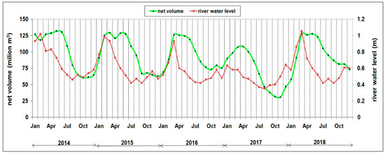
Figure 2.
Monthly averaged net volume of PL (green line) and water levels measured at the Grumento—Ponte La Marmora station (red line) for the investigated 2014–2018 period.
The above-mentioned hydrological variables are strongly interlinked and exhibit a well-defined seasonal cycle. In detail, the PL net volume (green line in Figure 2) is usually characterized by an initial refill from late winter to early spring (i.e., December–March), a high plateau phase from spring to early summer (with the maximum seasonal values), a subsequent drawdown during summer, and a final low plateau phase (with the minimum seasonal values) occurring from late summer to fall (i.e., August–November). All of these seasonal fluctuations mainly depend on discharge of the rivers affecting PL, such as the Agri River, which is one of the main rivers of the Basilicata region, entering the lake basin longitudinally from the west (Figure 1c). Other minor tributaries flow into PL, arising from both the northern (Spartifave, Rifreddo, Spetrizzone/Scannamogliera, Scazzero, and Grumentino rivers, only during the high-stand periods) and southern (Maglia, Vella, and Sciaura rivers during the high-stand periods) margins, with a typical torrential discharge regime [36] (Figure 1c). These tributaries drain areas composed of several detrital lithological units, thus determining different amounts and types of sediments at various locations in the reservoir [37].
2.2. In Situ Data Collection
Within the framework of the EU-funded SMART (Smart Cities and Communities and Social Innovation) BASILICATA project, six measurement campaigns were performed over the lake by sampling water and radiometric parameters at the station sites (Figure 1c) during the May 2017–May 2018 period (Table 1). The main goal of the measurement campaigns was to characterize the bio-optical properties of the area by homogenously sampling almost the whole lake. Each measurement campaign aimed to acquire data from the ten planned stations to better appreciate seasonal differences of in-water constituent concentrations (Figure 1c). Sub-surface (i.e., 0–1 m depth) water samples were acquired using Niskin bottles for subsequent laboratory measurements of TSM and chl-a concentrations and for absorption spectra analysis (i.e., Cromophoric Dissolved Organic Matter, CDOM). A total of 75 in situ measurements were acquired on the sampling stations as planned, for which the summary information is listed in Table 1. Simultaneously, above-water radiometric measurements (i.e., remote sensing reflectance Rrs (λ)) were acquired using a portable spectroradiometer to allow for the development and validation of a locally tuned TSM model.

Table 1.
Detailed information about the in situ measurement campaigns. The measurements were addressed to retrieve information on: total suspended matter—TSM, chlorophyll-a—chl-a, Cromophoric Dissolved Organic Matter absorption—aCDOM(440), and remote sensing reflectance—Rrs (λ).
For the above-mentioned measurements, a more detailed description of the TSM in situ and radiometric Rrs(λ) measurements is provided in the following paragraph.
In Situ TSM and Radiometric Rrs(λ)Measurements
Sub-surface water samples were collected in parallel to the spectral measurements and satellites overpasses by using Niskin bottles. The TSM concentration values of the collected samples were then determined gravimetrically according to Strickland & Parsons [38] and Joint Global Ocean Flux Study (JGOFS) protocols [39] in our laboratories. The water samples (500–1000 mL according to the number of particles) were filtered through 0.7 μm pre-weighed GF/F glass fiber filters (Whatman), washed with distilled water, and immediately dried in an oven at 100 °C. They were then re-weighed in the laboratory using a Mettler Toledo AG245 electronic balance with a detection limit of 0.1 mg.
In situ radiometric data were acquired from the deck of a boat (at 1 m height above lake surface) using a portable field spectroradiometer (i.e., FieldSpec FR PRO spectrometer, Analytical Spectral Devices (ASD), Boulder, CO, USA) equipped with a 8° foreoptic, following the National Aeronautics and Space Administration (NASA) ocean optics protocols for satellite ocean-color sensor validation [40]. The spectral characteristics of the above-mentioned instrument are suitable for measuring inland water optical properties in the visible domain, thanks to its 3 nm full-width at half-maximum (FWHM) and spectral sampling (i.e., 1 nm). Sky and water leaving radiances were acquired and normalized through a gray (30% albedo) panel (standard Spectralon, Labsphere, NH, USA), reasonably assumed to have a near-Lambertian behavior, and used to estimate the downwelling spectral irradiance (Es(λ)). In detail, the radiometer was alternately pointed downward to view the lake and upward to view the sky at the required [40] zenith angle (45°) and azimuth angle (90° or 180°). Furthermore, the spectroradiometer was equipped with a goniometer to derive the azimuth angle with respect to the sun’s azimuth angle, and with a bubble to ensure the correct zenith angle. After each set of radiance measurements (in our case, 10 measurements) towards the lake and sky were taken, the radiometer acquired the radiance derived by the horizontal gray panel. To take into account the signal spatial variability, multiple spectra (i.e., five at least) were acquired at the planned stations and averaged for each measurement station. Moreover, to minimize possible sources of noise, Rrs(λ) spectra affected by suspect acquisition conditions (i.e., variable light conditions, cloud coverage, and wind velocity higher than 5 m/s) were discarded, and thus did not influence the averaged spectrum magnitude. All the acquired spectra were then processed by using the ViewSpec Pro software 6.0 (ASD Inc., Boulder, CO, USA; [41]).
Such measurements aimed to retrieve the remote sensing reflectance Rrs(λ) (sr−1), defined as the ratio between the water leaving radiance Lw(ϴ,ϕ,λ) and the downwelling spectral irradiance Es(λ) [42]. The Rrs(λ) was calculated as
where Lw(ϴ,ϕ,λ) is the water leaving radiance (Wm−2nm−1sr−1) and Es(λ) is the above-surface downwelling spectral irradiance (Wm−2nm−1). The computation of these two variables was performed according to the standard protocols of ocean optics, as discussed in Zibordi et al. [43].
For instance, Figure 3 shows the Rrs(λ) spectra acquired by spectrometer with the relative TSM concentration values determined in the laboratory, over PL on 26 May 2017.
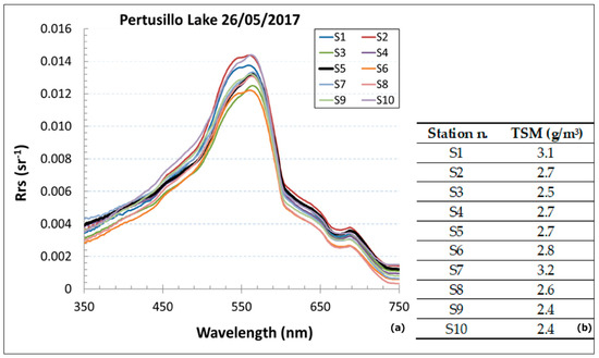
Figure 3.
(a) Rrs spectra acquired over PL on 26 May 2017 using the ASD spectrometer, and (b) the relative TSM concentration values determined in laboratory.
2.3. Satellite Data
To create a multi-year merged-satellite dataset, MSI and OLI data were analyzed in this work. MSI is a 13 band imager with a 10–60 m spatial resolution in the 440–2202 nm spectral domain [44], while OLI has a spatial resolution of 30 m (with nine bands) in the same spectral range (Table 2); thus, both are suitable for the assessment of lake ecosystem dynamics [45].
Table 2.
Central band wavelengths (nm) for the bands of the MSI and OLI sensors used in this work. Numbers in brackets represent the band spatial resolution (m). The panchromatic and cirrus bands of OLI and the cirrus and vapor bands of MSI were not considered. Near Infrared (NIR) and Shortwave Infrared (SWIR) bands are also indicated.
In detail, Level-1T (L1T) OLI and Level-1C (L1C) MSI data, containing geo-located and radiometrically calibrated top of atmosphere (TOA) reflectance, were obtained from the United States Geological Survey (USGS) web portal [46] and ESA’s science hub [47], respectively. Assuming that MSI-S2B data concurrent with the measurement campaigns were not available, only MSI-L1C data were downloaded for the 2016–2018 period. At the same time, the downloading process allowed all the OLI-L1T data available within the 2014–2018 temporal range to be collected (OLI data were available for all months since 2014).
All MSI-L1 data were re-sampled on a homogeneous grid with cells of 30 m spatial resolution and processed to obtain the derived L2 products (i.e., geophysical parameters such as Rrs(λ)) through the ACOLITE software [48], an open-access tool for atmospherically correcting and processing both Landsat-8 and Sentinel-2 data, especially for aquatic remote-sensing applications. A total of 164 MSI and 64 OLI cloud-free images (related to the 2016–2018 and 2014–2018 time periods, respectively) were exploited to develop the combined MSI–OLI TSM dataset.
Atmospheric Correction and Data-Processing Scheme
Starting from L1 data (L1T or L1C), the atmospheric correction was performed through two consecutive steps. The first one, namely the Rayleigh correction, allowed air molecule scattering to be accounted for by adopting a look-up table (LUT) derived from the 6SV radiative-transfer model [49]. Such a model needs different atmospheric parameters, such as the atmospheric pressure P(z), the amount of ozone O3, and water vapor H2O. P(z) was derived from a combination of data obtained from a coarse resolution (one deg., six hours time step) weather prediction model available from the Global Data Assimilation System (GDAS), while sea-level pressure, Psl, and the altitude, z (km), were given by a digital elevation model at 0.05 degree resolution [49]. The O3 and H2O amounts are provided by the GDAS via the ancillary information included in the MODIS surface-reflectance climate modeling grid (MOD09CMA) [49]. The second step towards the atmospheric correction implementation was aerosol correction, and was carried out through the implementation of the multi-band “dark spectrum fitting” technique (DSF) proposed by Vanhellemont & Ruddick [50]. The DSF method is inherently developed to identify pixels in a scene with sea surface reflectance ρs ≈ 0 in at least one of the sensor bands, where the atmospheric path reflectance (ρpath) can be estimated and considered constant over the scene of interest [51]. The input to the DSF method is the sensor TOA reflectance ρTOA(λ), from which the “dark spectrum” ρdark(λ) is identified and used to select the best fitting band and aerosol model combination to retrieve ρpath(λ). Considering that DSF identifies the band that gives the lowest ρpath estimation, pixels and bands with high sun glint were excluded from the ρpath computation process. For this reason, a sun glint correction was subsequently applied to the MSI–OLI data using a SWIR-and-based threshold approach (pixels with ρs at 1600 nm <0.11 were involved in the glint correction) through a semi-automatic procedure (user-specified) available in the ACOLITE tool.
After carrying out the atmospheric and glint corrections, a non-water masking was performed to exclude land or cloudy pixels from L2 data processing. The masking was carried out by using a fixed threshold of 2.15% on ρs at 1600 nm to exclude non-water pixels from further processing. The data processing ended with the estimation of L2 products, such as Rrs(λ), that were the input variables for the TSM model. The whole data-processing scheme is summarized in the flowchart shown in Figure 4.
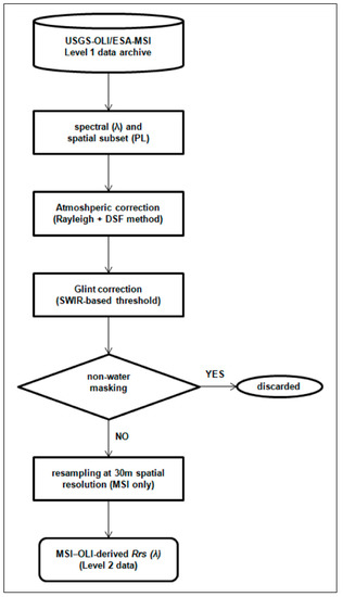
Figure 4.
Rrs(λ) Level 2 data-processing flowchart.
2.4. Comparison between Satellite and In Situ Data
The comparison between satellite and in situ data regarded the accuracy assessment of satellite-derived Rrs(λ) as well as the validation of a locally tuned TSM model. To these aims, in situ Rrs(λ) measurements acquired only in the absence of cloud coverage and with a low wind velocity (not higher than 5 m/s) were retained for satellite–in situ match-up analysis. Furthermore, it is worth specifying the spatial and temporal criteria adopted for the above-mentioned analysis. Satellite Level 2 data were averaged on a 3 × 3 pixel box centered on the location of in situ measurements, and only boxes containing at least 50% valid pixels were retained for match-up analysis [52]. Although the standard temporal criterion of a ±3 h time window around the satellite overpasses is usually adopted for in situ water sampling [52], we prudently scheduled them for ±1 h, thus ensuring that atmospheric conditions can be reasonably assumed to be even more stable.
The accuracy assessment was based on some regression indices and statistical indicators such as the determination coefficient (R2), the average ratio of satellite-to-in-situ data (r), the average absolute (unsigned) percent difference (APD), and the root-mean-square error (RMSE). The definitions of r, APD, and RMSE are given by the following equations, wherein xi is the ith satellite-derived value (or modeled by the regression analysis), yi is the ith in situ-derived value, and N is the number of samples selected.
Furthermore, the Nash–Sutcliffe efficiency (NSE) was used to evaluate the robustness of the locally tuned TSM model [53]. NSE is computed by the following equation, wherein TSMyi is the ith observed value of the dependent variable, TSMxi is the corresponding predicted value of the dependent variable given by the calibrated model, and TSMyi_mean is the mean observed value of the dependent variable [53].
The open-source statistical software R ver. 3.3.1 [54] was used for all the statistical analyses.
2.5. TSM Modeling Using MSI–OLI Combined Data
The TSM modeling via the combined use of MSI–OLI data consisted of two main consecutive steps, namely the development of a customized TSM model and the intersensor calibration process. The first phase aimed at local-scale tuning of an already existing empirical TSM algorithm or, alternatively, at developing a new customized TSM model. For this reason, we first evaluated the accuracy of an empirical TSM algorithm, namely the one developed by Nechad et al. [55]. This algorithm has been successfully tested worldwide, as its configuration allows for adjustment to different sensors or bands [56]. It is based on the use of a single band in the Red-to-NIR spectral range (within a TSM range of 0–100 g/m3), and it can be defined by the following Equation [55].
where ρw(λ) is the water leaving reflectance (in the Red or NIR band), and Ap(λ) and Cp(λ) are sensor-specific coefficients (specifically calibrated for the MSI and OLI sensors in September 2016) [48]. Considering the low–moderate turbid conditions of PL waters (i.e., with a maximum in situ TSM value of ~7 g/m3), we used the available Red bands (see Figure 3a) to implement the above-mentioned TSM algorithm, as the use of these bands is suitable for TSM values up to 50 g/m3 [9]. The Nechad et al. [55] algorithm tuning and the customized TSM model development were both based on the selection of two homogenous but independent datasets, namely the calibration and validation ones, characterized by the same percentage of summer and autumn stations (randomly selected) and that fitted the above-mentioned match-up criteria (see Section 2.4).
Finally, the proposed locally tuned TSM model was exported to OLI-L8 data to enlarge the dataset of analysis up to 2014, thus providing more cloud-free images (MSI–OLI merged dataset) useful to better investigate the multi-year TSM variability in PL. To this aim, we performed an intercalibration procedure that aimed to switch from the MSI-S2A Red band to the corresponding OLI-L8 one.
3. Results
3.1. Accuracy Assessment of MSI-Derived Rrs(λ)
The accuracy of the DSF atmospheric correction was assessed through the comparison between the MSI-Rrs(λ) and the corresponding in situ measurements, considering that no OLI overpasses were concurrent with the in situ sampling dates. Furthermore, only MSI-Rrs(λ) data acquired on 14 June 2017 and 12 October 2017 fitted with the above-mentioned temporal criterion (i.e., ±3 h), thus making them available for such an analysis. Figure 5 shows the results of the match-up analysis between MSI and in situ Rrs(λ) measurements for the first five MSI bands (i.e., 443, 492, 560, 665, and 704 nm), because of very low radiance values at wavelengths ≥ 700 nm (due to the strong water absorption at these wavelengths). The DSF atmospheric correction performed generally well for PL, as evidenced by the high R2 (0.95) with a statistically significant p-value < 0.001. The MSI-derived Rrs(λ) tended to slightly underestimate the simultaneous in situ Rrs(λ) (with r = 0.88) (Figure 5a). Referring to the MSI wavelengths, it is worth considering that the relative statistical errors at 443 nm, 492 nm, 560 nm, 665 nm, and 704 nm were less than 30% (i.e., APD values in Figure 5b). In particular, the Red bands (665 nm and 704 nm) showed the best accuracy (i.e., APD less than 10%), with RMSE values ranging between 0.29 and 00.36 × 10⁻³ sr–1, which was small enough to consider using these bands within a long-term trending analysis.
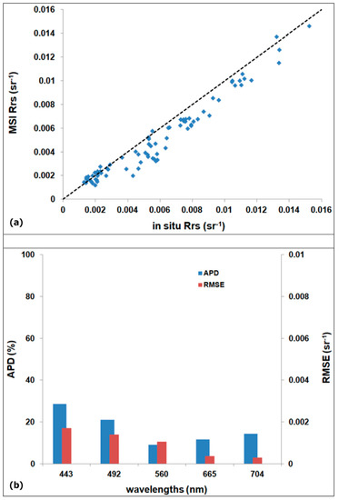
Figure 5.
(a) Scatter plot of in situ versus MSI-S2A derived Rrs(λ) values for the 443–704 nm spectral range. In the plot, the dashed line is the 1:1 line. (b) Histogram of error indicators (APD and RMSE) for the first five MSI-S2A bands (i.e., 443, 492, 560, 665, and 704 nm).
This results, namely the best performance of the DSF atmospheric correction at 665 nm and 704 nm, combined with the well-known high sensitivity of Red bands to TSM (up to 50 g/m3) [9], suggested the implementation of a model based on these MSI bands for TSM retrieval.
3.2. Calibration and Validation of a Locally Tuned TSM Model
The implementation of the Nechad et al. [55] algorithm for TSM retrieval (not shown for sake of brevity) at both the MSI-Red bands (665 and 704 nm) produced an unsatisfactory accuracy in terms of TSM concentration (0.57 < R2 < 0.72, 90.56% < APD < 105.98%, 1.4 g/m3 < RMSE < 1.85 g/m3). Therefore, we chose to develop a customized TSM model based on an MSI-Red band, rather than tuning at PL-scale the existing empirical algorithm by Nechad et al. [55]. Among the mathematical functions (i.e., linear, power law, logarithmic, exponential) used to establish the relationships between in situ Rrs(Red) and TSM data within the calibration dataset, the exponential function ensured the best performance, producing R2 values of 0.72 (p-value < 0.001) at Rrs(665) and 0.78 (p-value < 0.001) at Rrs(704) (Figure 6a,b).
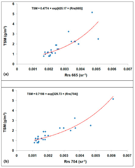
Figure 6.
(a) Calibration of the TSM model based on Rrs at 665 nm. (b) Calibration of the TSM model based on Rrs at 704 nm. In the plots, the superimposed equations are the exponential “best-fitting” functions (dashed red line).
The two TSM models proposed are defined by the following Equations (7) and (8).
Both the locally tuned TSM models ensured an acceptable robustness, as NSE values were 0.6 and 0.85 for the MSI Rrs(665)- and MSI Rrs(704)-based models, respectively. Within the validation dataset, the two models performed well, exhibiting a determination coefficient R2 of 0.81 and 0.84 (with p-values < 0.001), respectively. Furthermore the estimated TSM values were quite evenly distributed along the 1:1 dashed line, although they generally showed a slight underestimation, detectable by the r value range between 0.86 and 0.90, as showed in Figure 7a,b. Considering the same validation dataset, the Nechad et al. [55] TSM algorithm at both the MSI-Red bands (665 and 704 nm) confirmed the unsatisfactory performance in terms of TSM retrieval by exhibiting a clear overestimation (r value ranging between 1.57 and 1.85), as shown in Figure 7c,d.
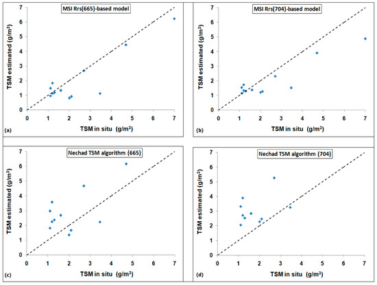
Figure 7.
TSM match-up analysis within the validation dataset. (a) TSM model based on Rrs at 665 nm. (b) TSM model based on Rrs at 704 nm. (c) Nechad et al. [55] TSM algorithm based on Rrs at 665 nm. (d) Nechad et al. [55] TSM algorithm based on Rrs at 704 nm. The dashed line is the 1:1 line.
Within a comparative analysis, the error metrics recorded by the two customized TSM models proposed and the Nechad et al. [55] TSM algorithms (at 665 nm and 704 nm) are summarized in Table 3.
Table 3.
Error metrics of the two customized TSM models and the Nechad et al. [55] TSM algorithms.
Both the customized TSM models proposed showed a significantly better accuracy in terms of TSM retrieval (APD and RMSE values in Table 3), thus confirming them to be more suitable than the existing [55] TSM algorithms for these site-specific conditions. Although the MSI Rrs(704)-based exponential model (defined by Equation (8)) showed a good performance (R2 = 0.78 with p-value < 0.001) within the calibration dataset and a slightly better accuracy in the validation phase (R2 = 0.84, APD = 26% and RMSE = 0.95 g/m3), we adopted the locally tuned TSM model based on Rrs at 665 nm in order to make it exportable (through an intercalibration process) to the OLI sensor, considering that 704 nm is out of range for the OLI sensor’s spectral configuration (this sensor is characterized by a single Red band in the 630–680 nm spectral domain).
3.3. Intercalibration between MSI and OLI
Considering that S2A and L8 are placed in orbits that allow for occasional near-simultaneous collections, we analyzed, within the 2014–2018 period, 4 days (i.e., 5 October 2017, 24 December 2017, 21 August 2018, and 9 November 2018) characterized by acquisition time difference < 30 min. In detail, we plotted the MSI Rrs(665) with the concurrent OLI Rrs(655) in order to find the “best-fitting” function between the two variables. The linear function was defined by the following Equation (9).
Figure 8 shows the scatterplot obtained for all the available water and cloud-free pixels (N = 11,977).
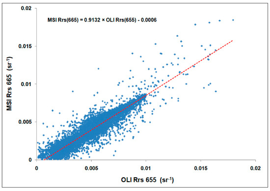
Figure 8.
Scatter plot of MSI-S2A-derived Rrs(665) and OLI-L8-derived Rrs(655) for all the water pixels available (N = 11,977) within the 4 days considered. The superimposed equation is the linear “best-fitting” function (dashed red line).
The linear “best-fitting” function exhibited the best performance, recording the highest determination coefficient (R2 = 0.87; p-value < 0.001) and a RMSE value of 0.1 × 10⁻² sr−1 on OLI Rrs(655) data (Figure 8). The proposed intercalibration procedure ensured the implementation of the MSI Rrs(665)-based TSM model on OLI Rrs(655) data as well, thus allowing for the development of a multi-year (2014–2018) MSI–OLI combined dataset of TSM retrievals.
3.4. Seasonal TSM Variations
Based on the MSI–OLI combined TSM dataset for the 2014–2018 period, we generated multi-year (2014–2018) TSM monthly averaged maps (i.e., 2014–2018 January TSM mean, 2014–2018 February TSM mean, etc.), as shown in Figure 9, to evaluate the seasonal TSM fluctuations and their spatial patterns.
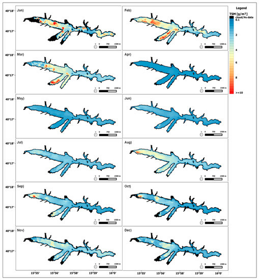
Figure 9.
The multi-year (2014–2018) TSM monthly averaged maps for each calendar month. Black pixels correspond to non-water, cloudy, or missed data.
Looking at the TSM monthly averaged maps in Figure 9, the winter and early spring TSM maps (i.e., from January to March) showed the highest TSM concentration values (up to about 10 g/m3) especially on the south-western side of PL. Moving from spring to early summer (from April to June), TSM values lower than 2 g/m3 were observed over the whole PL area. Finally, the summer and fall seasons showed a subsequent general increase in TSM concentration (with values ranging between 5 and 8 g/m3), probably due to water level fluctuations occurring in this seasonal period [29].
To better identify sub-regions characterized by similar TSM spatial dynamics within the seasonal trend, we performed a classification analysis. The ISODATA (Iterative Self-Organizing Data Analysis technique) non-supervised classification scheme [57] was implemented, entering as “in input spectral bands” the already computed multi-year (2014–2018) TSM monthly means of each calendar month (i.e., the 12 maps in Figure 9). In detail, the unsupervised ISODATA classification iteratively calculates the “spectral” mean of each identified class, and then iteratively clusters the remaining pixels using the minimum-distance technique. During each iteration, the process recalculates the means and reclassifies pixels with respect to the new ones, by setting user-defined threshold parameters, such as the maximum number of iterations (set to 10) and the change threshold (equal to 10%). The map obtained by the ISODATA non-supervised classification, shown in Figure 10, is an original output of this work that could be used in future for better definition of the in situ stations to be sampled.
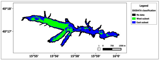
Figure 10.
Map resulting from the ISODATA (Iterative Self-Organizing Data Analysis technique) non-supervised classification.
Looking at the map in Figure 10, it is worth recognizing the two sub-regions (namely the “West” and “East” subsets), probably characterized by differences due to amount of sediment or magnitude of hydrological forcing. The West subset (depicted in green in Figure 10) encompassed the south-western side of the lake mostly affected by river discharges, considering the Agri River longitudinal outflow as well as the southern outflow of minor tributaries such as Maglia and Vella (see Figure 1c). The East region (blue in Figure 10) was the complementary eastern side of the lake and it is probably characterized by a reduced amount of suspended matter, considering the marginal influence of river discharges. In this scenario, we separately analyzed the western and eastern subsets, computing the 2014–2018 TSM seasonal cycle spatially averaged over each sub-region identified, as shown in Figure 11.
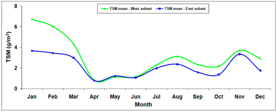
Figure 11.
The 2014–2018 TSM seasonal cycles spatially averaged over the West and East subsets, depicted by continuous green and blue lines, respectively.
Both the defined sub-regions showed almost comparable seasonal patterns (especially from April to December), although the West subset generally showed higher TSM values during most of the months. In detail, the most significant differences between the two sub-regions were observed in the winter season, when the West subset showed TSM spatially averaged values clearly higher than those recorded in the East one (by on average about 2 g/m3). Conversely, within the April–June period, it is worth noting that there were no appreciable discrepancies between the two sub-areas, which was speculated to be because that the constantly high value of PL’s net volume tends to determine lower detectable TSM values homogenously over the whole lake.
Although the above-mentioned hydrological parameters could have mostly influenced the TSM seasonal dynamics over PL, it is worth considering the lake topography as another key factor influencing the TSM spatial patterns over these two sub-areas. To this end, we adopted the original bathymetry measured in September 2007 by Consiglio per la Ricerca e la Sperimentazione in Agricoltura—Centro per l’Agrobiologia e la Pedologia (CRA – ABP) [29], considering that no updated bathymetry maps were available. In this framework, we superimposed the above-mentioned bathymetry map with the September interannual (2014–2018) averaged TSM map (see Figure 9), assuming comparable geo-morphological conditions as much as possible. In detail, we analyzed the relationship between TSM variability and depth along the A–C transect, considering the ISODATA classification map as a background layer (Figure 10, Figure 12). The derived scatterplot in Figure 12d, obtained by averaging all the TSM values contained into each pixel at a constant depth, shows how TSM varied with depth for each sub-region identified (i.e., the green and blue dots represent the West and East areas, respectively).
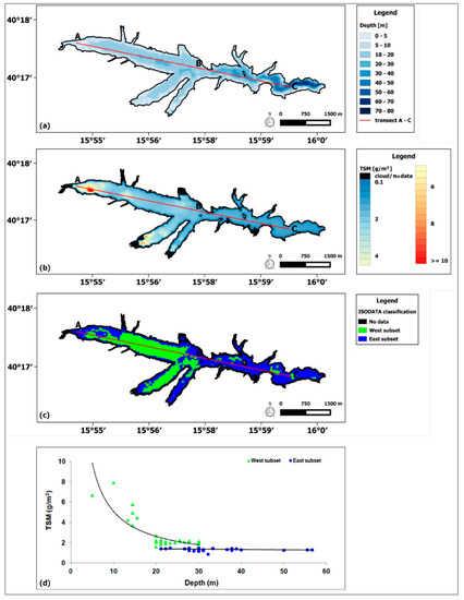
Figure 12.
(a) September 2007 bathymetry map adapted from CRA-ABP. The continuous red line is the A–C transect; (b) September interannual (2014–2018) averaged TSM map; (c) ISODATA unsupervised classification map; (d) Scatterplot of TSM and depth values along the A–C transect. The green triangles and the blue dots indicate the TSM–depth variations within the West and East subsets, respectively. The dashed and continuous lines are the best fit functions estimated for West and East areas, respectively.
Focusing on the West subset and especially along the A–B portion of the transect, the TSM concentration decreased with increasing depth, as depicted by the dashed black line in Figure 12d and according to a negative power law (R2 = 0.72; p-value < 0.001). Conversely, for the East subset (i.e., along the B-C portion of the transect), it was not worth defining a best fit function as the linear one (i.e., the continuous black line in Figure 12d) showed a very low R2 value (0.033) and a statistically non-significant p-value (0.04). Based on this analysis, it is reasonable to speculate that lake bathymetry is a relevant factor that influences mainly the western portion of PL, as TSM values did not vary with depth in the East subset.
4. Discussion
The assessment of TSM spatiotemporal variability plays a crucial role in inland water management, considering how these fluctuations influence water transparency, light availability, and the physical, chemical, and biological processes (such as primary production) [58,59,60]. New opportunities for monitoring certain quality parameters (e.g., chlorophyll-a, TSM) have emerged thanks to the suitability of medium-resolution multispectral sensors such as OLI and MSI, onboard the Landsat 8 and Sentinel-2 satellite platforms, respectively [61,62]. Furthermore, the joint use of these sensors offers the opportunity to build time series with an improved revisiting time [63], thus enabling limnologists, coastal oceanographers, aquatic ecologists, and water resource managers to enhance their monitoring efforts [64,65]. NASA scientists generated harmonized Landsat and Sentinel-2 (HLS) surface reflectance products [66] by proposing a method that creates global fixed per-band transformation coefficients to reduce the reflectance difference between Landsat 8 and Sentinel-2. Although the HLS products represent a free and useful opportunity to create MSI–OLI combined datasets, they do have some disadvantages that hamper their exploitation by the ocean-color community. In detail, the HLS products were mostly designed for land applications, and the atmospheric correction method adopted does not correct for the adjacency effect, one of the main issues concerning inland water applications using satellite data [67]. Furthermore, the harmonized dataset is available only for selected sites (120 worldwide), not allowing for a replication of the proposed approach everywhere in the world. In this framework, we evaluated the capability of MSI–OLI combined data in characterizing the TSM multi-year variability in PL.
4.1. TSM Model Calibration and Validation
The adoption of an adequate atmospheric correction method is a necessary preliminary step to develop an easily operational TSM model based on satellite data, as inland waters are usually affected by several issues (e.g., adjacency effects or optical heterogeneity of the atmosphere) that may invalidate the inherent assumptions on which marine atmospheric correction algorithms are based [68,69]. In addition, the optical complexity of inland waters generates a non-negligible water leaving reflectance in the NIR domain, which typically used to remove the atmospheric aerosol contribution (i.e., “black-pixel assumption” [70]). The “dark spectrum fitting” technique (DSF) [50], used in this work, starts from assumptions similar to those underlying the common atmospheric correction methods, such as the above-cited “black” water pixels in the NIR [70] and SWIR [71] regions. However, these hypotheses are combined in a novel way, as the DSF method does not consider a priori selection of the “black” band, but identifies the best-fitting band and aerosol model combination to retrieve the atmospheric path reflectance ρpath [50]. This dynamic band selection allows amplification of adjacency effects within the atmospheric correction to be avoided, considering that shifting from NIR or SWIR bands to less affected bands (e.g., Blue or Red) can produce a lower error on the ρpath estimation [50].
The regression indices and statistical indicators obtained by the match-up analysis between MSI-S2A-derived and in situ Rrs(λ) (R2 = 0.95 and RMSE value between 0.00029 and 0.00036 sr−1) proved the DSF scheme’s suitability for this study area, thus corroborating the results achieved by Vanhellemont [51] for more than 30 years of data from Landsat 5/7/8 to Sentinel-2A/B. The best accuracy of the atmospheric correction at 665 and 704 nm, namely the more suitable bands for TSM retrievals (up to 50 g/m3 [72]), allowed us to develop and validate a customized Red-band-based model to retrieve TSM concentrations by MSI-S2A data. Upon a deep analysis of the calibration phase, the high determination coefficients (ranging between 0.72 and 0.78) and the good values of NSE (ranging between 0.6 and 0.85) showed by the MSI Rrs(665)- and Rrs(704)-based exponential models were explained by the occurrence of low–moderate turbid waters (see values in Figure 3). The use of Red bands has been confirmed to be suitable for TSM estimations in such waters (i.e., up to 50 g/m3), where changes in TSM concentration cause a higher spectral response in VIS (i.e., especially in the 600–700 nm region) than in the NIR spectral domain [9]. Although both the locally tuned TSM models ensured a good accuracy within the validation phase, the acquisition of sampling data in all the seasonal conditions should lead to a higher TSM variability range and make the validation phase more statistically significant [73]. Furthermore, the dataset of in situ measurements should include further parameters useful to better characterize the bio-optical conditions of the study area. For instance, measurements of the Secchi disk depth (ZSD, m) and back-scattering coefficient bbp(λ) estimates can provide more detailed information about water transparency [74] and suspended particle size distribution and composition, respectively [75]. It is worth saying that while the methodological approach here proposed can be easily replicated in other geographic locations, the application of the derived TSM model as it is presented cannot be carried out without region-specific adaptation or calibration.
4.2. MSI–OLI Combined Dataset for TSM Seasonal Analysis
The subsequent exportation of an MSI-based TSM model to OLI data allowed the S2A-L8 satellite combination to be exploited, thus providing a general increase in the number of available observations and a revisit-time minimization [64]. In this case study, the addition of OLI data to the combined dataset resulted in a 30% increase in number of cloud-free images and an averaged revisit interval up to about 4 days for the summer months (characterized by more frequent cloud-free images) at PL coordinates (lat/lon). Furthermore, a time difference of about 18 min between near-simultaneous MSI–OLI collections (estimated average value for the 4 days analyzed) should have ensured similar atmospheric and water conditions, thus minimizing the sources of uncertainties and ensuring a more accurate intercomparison analysis [76]. In this framework, it is worth pointing out the high determination coefficient (R2 = 0.87; p-value < 0.001) showed by the linear best fit function between MSI Rrs(665) and the concurrent OLI Rrs(655). The statistical reliability of the intercalibration allowed us to create an MSI–OLI combined TSM dataset useful to investigate the seasonal TSM variability and its spatial dynamics.
The multi-year (2014–2018) TSM monthly maps derived from the MSI–OLI combined dataset indicated the influence of hydrological variables (i.e., rainfall, inflowing rivers, and net volume) on the TSM seasonal fluctuations. The torrential discharge regime of the inflowing rivers (i.e., Agri, Maglia, and Vella) induces an increase in TSM concentration from winter to early spring. Subsequently, the rainfall decreases and the constantly high net volume in spring causes a reduction in TSM concentration, while changes in net volume seem to affect the TSM increase during summer and fall. Although the assessment of the TSM seasonal variations already suggested the occurrence of a more exposed area (i.e., south-western area), the non-supervised classification provided a better characterization of the TSM spatial patterns thanks to the identification of two distinct sub-regions, namely the West and East areas. The seasonal analysis performed on these sub-areas further corroborated how much PL’s western side is affected by hydrological factors, the effects of which tend to longitudinally decrease. Conversely, PL’s eastern side probably reflects the absence of other main tributaries, thus showing smaller amounts of suspended matter. Upon a deep analysis, lake topography also proved to be a crucial factor affecting mainly the western portion of PL. This area, characterized by multiple longitudinal and lateral deltas, is strongly influenced by deposition and erosion phenomena [29], which usually occur in shallow lakes because of water level fluctuations [77,78,79]. For this reason, we speculate that the maximum water level drawdown occurring in the summer–fall season could lead to more frequent episodes of erosion and sediment resuspension in the deltaic and shallower West sub-area, with a consequent increase in TSM concentration.
4.3. Future Perspectives
This work allowed characterization of the TSM seasonal variability over PL and identification a sub-region more exposed to TSM fluctuations, especially in certain seasonal periods (i.e., winter and summer–fall). Such an achievement could be profitably exploited to support the WFD’s requested monitoring activities intended to ensure good quality status of water bodies. A monitoring program usually consists of three consecutive phases: (i) the surveillance, (ii) operational, and (iii) investigative phases. The surveillance step involves acquiring information on the initial qualitative status of water body, and the operational step involves assessing the suitability of the adopted monitoring actions. The investigative step is intended to detect possible sources of accidental pollution that could prevent the ecological goals being achieved [80]. Within the surveillance phase, the obtained results can be useful for regional environmental agencies in establishing the actions to be taken during the subsequent operational steps. The identification of the seasons more affected by high TSM values and the detection of a more susceptible area could contribute to defining the minimum number of sampling points, their location, and sampling frequency, thus facilitating the development of an adequate monitoring plan.
However, the present 5 year (2014–2018) period of study is not large enough to enable the assessment of long-term variations in water quality due to both natural and anthropogenic activities. Furthermore, the high environmental relevance of this reservoir suggests the need to extend the period of analysis in order to investigate possible changes in water quality before and after the occurrence of human-induced pressures (i.e., the oil extraction and pre-treatment activities carried out by ENI in the Agri Valley domain since 2001 [81]). To create a long-term combined dataset and characterize unperturbed PL conditions, it would be worth exporting this locally tuned TSM model to Landsat 5 Thematic Mapper (1984–2011) and Landsat 7 Enhance Thematic Mapper plus (1999–present), taking into account that these satellite-sensor systems show a suitable spectral configuration (i.e., similar Red bands to OLI-L8 system). Within the investigative monitoring phase, the subsequent development and implementation of a statistically based change detection index could enable the creation of an early detection tool useful for identifying any anomalous (within the space–time domain) TSM plumes. Furthermore, within the next 10–15 years, the potential constellation of OLI onboard Landsat-8/9 and MSI aboard Sentinel-2 missions will allow more than 40 years of merged data to be exploited for investigation of possible climate-related changes in PL. The very high observational frequency (i.e., ~2.9 days) guaranteed by this virtual constellation from 2021 (when Landsat-9 becomes operational) will also be essential to further reduce any acquisition gap [65].
5. Conclusions
In this study, we evaluated the potential of MSI–OLI combined data in characterizing the multi-year (2014–2018) TSM variability in Pertusillo Lake (Basilicata region, southern Italy).
By exploiting the DSF atmospheric correction method, an existing standard algorithm for TSM retrievals [55] was first implemented. The unsatisfactory accuracy produced by the above-mentioned TSM algorithm suggested the calibration and validation of a customized TSM model based on MSI data. Furthermore, the good performance of the DSF atmospheric correction method (R2 = 0.95 with p-value < 0.001), especially for the MSI Red bands (RMSE value ranging between 0.00029 and 0.00036 sr−1) enabled the development of a MSI Rrs(665)-based model for TSM retrievals. This locally tuned TSM model performed well within the validation dataset, exhibiting a determination coefficient R2 = 0.81 (with p-value < 0.001) and returning APD and RMSE values of 27.72% and 0.89 g/m3, respectively. The MSI-based TSM model was also exported to OLI data through an intercalibration process, the statistical reliability of which was proven by the high determination coefficient R2 = 0.87 (p-value < 0.001) of the linear “best-fitting” function. The intercalibration phase resulted in the creation of a multi-year (2014–2018) MSI–OLI combined dataset of TSM retrievals that enabled better investigation of the TSM seasonal variability in PL.
The derived multi-year TSM monthly maps showed the highest TSM concentration values (up to about 10 g/m3) during the winter–spring season, especially on the south-western side of PL; a spatially homogeneous decrease from spring to early summer (TSM values lower than 2 g/m3); and a new TSM increase during the summer and fall seasons (TSM values ranged between 5 and 8 g/m3). By means of the unsupervised ISODATA classification scheme, two distinct sub-regions, namely the West and East subsets, characterized by differences in the amount of sediment or the magnitude of hydrological forcing were identified. Furthermore, the achieved findings suggested the inherent influence of lake bathymetry on TSM values within PL’s western portion. In this framework, we speculate that the deltaic and shallower western side is more influenced by rainfall, inflowing rivers, and water level fluctuations, the effects of which tend to longitudinally decrease, thus resulting in smaller amounts of suspended matter within the low-energy eastern sub-area.
The results obtained in this work could be profitably used by regional and local authorities for better management of inland water quality (sediment infilling of the reservoir) and their monitoring system.
Author Contributions
E.C., T.L. and N.P. designed the research and developed the methodology. E.C. wrote most of the paper. A.C., A.P. and S.P (Simone Pascucci) collected and processed the in situ measurements. E.C. collected and processed MSI and OLI data. E.C. and V.S. performed the data analysis. E.C., N.P., T.L., S.P. (Stefano Pignatti) and S.P. (Simone Pascucci) contributed in interpreting results. N.P., T.L., S.P. (Simone Pascucci) and V.T. revised the manuscript. All authors have read and agreed to the published version of the manuscript.
Funding
This research was carried out in the framework of the project ‘Smart Basilicata’, which was approved by the Italian Ministry of Education, University and Research (Notice MIUR n.84/Ric 2012, PON 2007-2013 of 2 March 2012) and was funded with the Cohesion Fund 2007–2013 of the Basilicata Regional authority.
Acknowledgments
Colleagues from CNR IRBIM and CNR IMAA are gratefully acknowledged for stimulating discussions and constructive support throughout the SMART BASILICATA project, from conception to implementation. Serena Sabia from CNR IMAA is thanked for her help in the laboratory samples preparation.
Conflicts of Interest
The authors declare no conflict of interest.
References
- Vörösmarty, C.J.; McIntyre, P.B.; Gessner, M.O.; Dudgeon, D.; Prusevich, A.; Green, P.; Davies, P.M. Global Threats to Human Water Security and River Biodiversity. Nature 2010, 467, 555–561. [Google Scholar] [CrossRef]
- Adrian, R.; O’Reilly, C.M.; Zagarese, H.; Baines, S.B.; Hessen, D.O.; Keller, W.; Livingstone, D.M.; Sommaruga, R.; Straile, D.; Van Donk, E.; et al. Lakes as Sentinels of Climate Change. Limnol. Oceanogr. 2009, 54, 2283–2297. [Google Scholar] [CrossRef] [PubMed]
- Stendera, S.; Adrian, R.; Bonada, N.; Cañedo-Argüelles, M.; Hugueny, B.; Januschke, K.; Pletterbauer, F.; Hering, D. Drivers and Stressors of Freshwater Biodiversity Patterns Across Different Ecosystems and Scales: A Review. Hydrobiologia 2012, 696, 1–28. [Google Scholar] [CrossRef]
- Hering, D.; Borja, A.; Carstensen, J.; Carvalho, L.; Elliott, M.; Feld, C.K.; Heiskanen, A.S.; Johnson, R.K.; Moe, J.; Pont, D.; et al. The European Water Framework Directive at the Age of 10: A Critical Review of the Achievements with Recommendations for the Future. Sci. Total Environ. 2010, 408, 4007–4019. [Google Scholar] [CrossRef] [PubMed]
- Novoa, S.; Doxaran, D.; Ody, A.; Vanhellemont, Q.; Lafon, V.; Lubac, B.; Gernez, P. Atmospheric Corrections and Multi-Conditional Algorithm for Multi-Sensor Remote Sensing of Suspended Particulate Matter in Low-to-High Turbidity Levels Coastal Waters. Remote Sens. 2017, 9, 61. [Google Scholar] [CrossRef]
- Doxaran, D.; Lamquin, N.; Park, Y.J.; Mazeran, C.; Ryu, J.H.; Wang, M.; Poteau, A. Retrieval of the Seawater Reflectance for Suspended Solids Monitoring in the East China Sea Using MODIS, MERIS and GOCI Satellite Data. Remote Sens. Environ. 2014, 146, 36–48. [Google Scholar] [CrossRef]
- Zhu, M.Y.; Zhu, G.W.; Li, W.; Zhang, Y.L.; Zhao, L.L.; Gu, Z. Estimation of the Algal-Available Phosphorus Pool in Sediments of a Large, Shallow Eutrophic Lake (Taihu, China) Using Profiled SMT Fractional Analysis. Environ. Pollut. 2013, 173, 216–223. [Google Scholar] [CrossRef]
- Nguyen, H.L.; Leermakers, M.; Osan, J.; Torok, S.; Baeyens, W. Heavy Metals in Lake Balaton: Water Column, Suspended Matter, Sediment and Biota. Sci. Total Environ. 2005, 340, 213–230. [Google Scholar] [CrossRef]
- Di Polito, C.; Ciancia, E.; Coviello, I.; Doxaran, D.; Lacava, T.; Pergola, N.; Tramutoli, V. On the Potential of Robust Satellite Techniques Approach for SPM Monitoring in Coastal Waters: Implementation and Application Over the Basilicata Ionian Coastal Waters Using MODIS-Aqua. Remote Sens. 2016, 8, 922. [Google Scholar] [CrossRef]
- Giardino, C.; Bresciani, M.; Stroppiana, D.; Oggioni, A.; Morabito, G. Optical Remote Sensing of Lakes: An Overview on Lake Maggiore. J. Limnol. 2014, 73, 201–214. [Google Scholar] [CrossRef]
- Shi, K.; Zhang, Y.; Zhu, G.; Liu, X.; Zhou, Y.; Xu, H.; Li, Y. Long-Term Remote Monitoring of Total Suspended Matter Concentration in Lake Taihu Using 250 m MODIS-Aqua Data. Remote Sens. Environ. 2015, 164, 43–56. [Google Scholar] [CrossRef]
- Dörnhöfer, K.; Göritz, A.; Gege, P.; Pflug, B.; Oppelt, N. Water Constituents and Water Depth Retrieval from Sentinel-2A—A first Evaluation in an Oligotrophic Lake. Remote Sens. 2016, 8, 941. [Google Scholar] [CrossRef]
- Doxaran, D.; Castaing, P.; Lavender, S.J.; Castaign, P.; Lavender, S.J. Monitoring the Maximum Turbidity Zone and detecting Fine Scale Turbidity Features in the Gironde estuary Using High Spatial Resolution Satellite Sensor (SPOT HRV, Landsat ETM) Data. Int. J. Remote Sens. 2006, 27, 2303–2321. [Google Scholar] [CrossRef]
- Miller, R.L.; McKee, B.A. Using MODIS Terra 250 m Imagery to Map Concentrations of Total Suspended Matter in Coastal Waters. Remote Sens. Environ. 2004, 93, 259–266. [Google Scholar] [CrossRef]
- Feng, L.; Hu, C.; Chen, X.; Song, Q. Influence of the Three Gorges Dam on Total suspended Matters in the Yangtze Estuary and its Adjacent Coastal Waters: Observations from MODIS. Remote Sens. Environ. 2014, 140, 779–788. [Google Scholar] [CrossRef]
- Petus, C.; Marieu, V.; Novoa, S.; Chust, G.; Bruneau, N.; Froidefond, J.M. Monitoring Spatio-Temporal Variability of the Adour River Turbid Plume (Bay of Biscay, France) with MODIS 250-m Imagery. Cont. Shelf Res. 2014, 74, 35–49. [Google Scholar] [CrossRef]
- Palmer, S.; Odermatt, D.; Hunter, P.D.; Brockmann, C.; Présing, M.; Balzter, H.; Tóth, V.R. Satellite Remote Sensing of Phytoplankton Phenology in Lake Balaton Using 10 years of MERIS Observations. Remote Sens. Environ. 2015, 158, 441–452. [Google Scholar] [CrossRef]
- Binding, C.E.; Greenberg, T.A.; Watson, S.B.; Rastin, S.; Gould, J. Long Term Water Clarity Changes in North America’s Great Lakes from Multi-Sensor Satellite Observations. Limnol. Oceanogr. 2015, 60, 1976–1995. [Google Scholar] [CrossRef]
- Kiefer, I.; Odermatt, D.; Anneville, O.; Wüest, A.; Bouffard, D. Application of Remote Sensing for the Optimization of In-Situ Sampling for Monitoring of Phytoplankton Abundance in a Large Lake. Sci. Total Environ. 2015, 527, 493–506. [Google Scholar] [CrossRef] [PubMed]
- Palmer, S.C.; Kutser, T.; Hunter, P.D. Remote Sensing of Inland Waters: Challenges, Progress and Future Directions. Remote Sens. Environ. 2015, 157, 1–8. [Google Scholar] [CrossRef]
- Dörnhöfer, K.; Oppelt, N. Remote Sensing for Lake Research and Monitoring—Recent Advances. Ecol. Indic. 2016, 64, 105–122. [Google Scholar] [CrossRef]
- Gernez, P.; Doxaran, D.; Barillé, L. Shellfish Aquaculture from Space: Potential of Sentinel2 to Monitor Tide-Driven Changes in Turbidity, Chlorophyll Concentration and Oyster Physiological Response at the Scale of an Oyster Farm. Front. Mar. Sci. 2017, 4, 137. [Google Scholar] [CrossRef]
- Liu, H.; Li, Q.; Shi, T.; Hu, S.; Wu, G.; Zhou, Q. Application of Sentinel 2 MSI Images to Retrieve Suspended particulate matter concentrations in Poyang Lake. Remote Sens. 2017, 9, 761. [Google Scholar] [CrossRef]
- Toming, K.; Kutser, T.; Laas, A.; Sepp, M.; Paavel, B.; Nõges, T. First Experiences in Mapping Lake Water Quality Parameters with Sentinel-2 MSI Imagery. Remote Sens. 2016, 8, 640. [Google Scholar] [CrossRef]
- Eder, E.; Dörnhöfer, K.; Gege, P.; Schenk, K.; Klinger, P.; Wenzel, J.; Gruber, N. Analysis of Mineral-Rich Suspended Matter in Glacial Lakes Using Simulations and Satellite Data. In Living Planet Symposium; Ouwehand, L., Ed.; ESA Communications: Noordwijk, The Netherlands, 2016; Volume 740. [Google Scholar]
- Manzo, C.; Bresciani, M.; Giardino, C.; Braga, F.; Bassani, C. Sensitivity Analysis of a Bio-Optical Model for Italian Lakes Focused on Landsat-8, Sentinel-2 and Sentinel-3. Eur. J. Remote Sens. 2015, 48, 17–32. [Google Scholar] [CrossRef]
- Lavrova, O.Y.; Soloviev, D.M.; Strochkov, M.A.; Bocharova, T.Y.; Kashnitsky, A.V. River plumes investigation using Sentinel-2A MSI and Landsat-8 OLI data. In Remote Sensing of the Ocean, Sea Ice, Coastal Waters, and Large Water Regions; International Society for Optics and Photonics: Bellingham, WA, USA, 2016; Volume 9999, p. 99990G. [Google Scholar]
- Pahlevan, N.; Chittimalli, S.K.; Balasubramanian, S.V.; Vellucci, V. Sentinel-2/Landsat-8 Product Consistency and Implications for Monitoring Aquatic Systems. Remote Sens. Environ. 2019, 220, 19–29. [Google Scholar] [CrossRef]
- Colella, A.; Fortunato, E. The Sedimentary Infill of the Pertusillo Freshwater Reservoir (Val d’Agri, Southern Italy). Feb Fresenius Environ. Bull. 2019, 23, 824–830. [Google Scholar]
- Faruolo, M.; Coviello, I.; Filizzola, C.; Lacava, T.; Pergola, N.; Tramutoli, V. A Satellite-Based Analysis of the Val d’Agri Oil Center (Southern Italy) Gas Flaring Emissions. Nat. Hazards Earth Syst. Sci. 2014, 14, 2783–2793. [Google Scholar] [CrossRef]
- D’Emilio, M.; Coluzzi, R.; Macchiato, M.; Imbrenda, V.; Ragosta, M.; Sabia, S.; Simoniello, T. Satellite Data and Soil Magnetic Susceptibility Measurements for Heavy Metals Monitoring: Findings from Agri Valley (Southern Italy). Environ. Earth Sci. 2018, 77, 63. [Google Scholar] [CrossRef]
- Yao, Z.; Gao, P. Heavy Metal Research in Lacustrine Sediment: A Review. Chin. J. Oceanol. Limnol. 2007, 25, 444–454. [Google Scholar] [CrossRef]
- Simoniello, T.; Coluzzi, R.; Imbrenda, V.; Lanfredi, M. Land Cover Changes and Forest Landscape Evolution (1985–2009) in a Typical Mediterranean Agroforestry System (High Agri Valley). Nat. Hazards Earth Syst. Sci. Discuss. 2015, 3. [Google Scholar] [CrossRef]
- Autorità Di Bacino Della Basilicata. Available online: http://www.adb.basilicata-it/adb/risorseidriche/diaginv.asp?invaso=Pertusillo (accessed on 18 May 2020).
- Centro Funzionale Basilicata. Available online: http://centrofunzionalebasilicata.it/it/scaricaDati (accessed on 18 May 2020).
- Capozza, F. Influenza del fattore geomorfologico e litoloco sul trasporto solido del Fiume Agri a monte della diga del Pertusillo. Rass. Lav. Pubblici 1963, 12, 1235–1258. [Google Scholar]
- Anselmi, B.; Blasi, L.; Cautilli, F.; Crovato, C.; Grauso, S. La sedimentazione nell’invaso artificiale del Pertusillo (Fiume Agri, Basilicata). Geol. Tec. Ambient. 1996, 4, 19–34. [Google Scholar]
- Strickland, J.D.; Parsons, T.R. A Practical Handbook of Seawater Analysis; Journal of Fisheries Research Board of Canada: Ottawa, ON, Canada, 1972. [Google Scholar]
- UNESCO. Protocols for the Joint Global Ocean Flux Study (JGOFS) Core Measurements; UNESCO-IOC: Paris, France, 1994. [Google Scholar]
- Mueller, J.L.; Fargion, G.S.; McClain, C.R. Ocean Optics Protocols for Satellite Ocean Color Sensor Validation. In Technical Memorandum TM-2003-21621/Revision 5; NASA Goddard Space Flight Space Center: Greenbelt, MD, USA, 2004. [Google Scholar]
- ViewSpec Pro Software Manual, ASD Inc. 2008. Available online: http://www.grss-ieee.org/lep4/project_materials_for_web/viewspecpro_manual.pdf (accessed on 18 May 2020).
- Lee, Z. Remote Sensing of Inherent Optical Properties: Fundamentals, Tests of Algorithms, and Applications; International Ocean-Colour Coordinating Group: Hanover, NH, Canada, 2006; Volume 5. [Google Scholar]
- Zibordi, G.; Voss, K. Protocols for Satellite Ocean Color Data Validation: In Situ Optical Radiometry; IOCCG Protocols Document; IOCCG: Hanover, NH, Canada, 2019. [Google Scholar]
- Coluzzi, R.; Imbrenda, V.; Lanfredi, M.; Simoniello, T. A First Assessment of the Sentinel-2 Level 1-C Cloud Mask Product to Support Informed Surface Analyses. Remote Sens. Environ. 2018, 217, 426–443. [Google Scholar] [CrossRef]
- Vanhellemont, Q.; Ruddick, K. Acolite for Sentinel-2: Aquatic applications of MSI imagery. In Proceedings of the 2016 ESA Living Planet Symposium, Prague, Czech Republic, 9–13 May 2016; pp. 9–13. [Google Scholar]
- United States Geological Survey (USGS) Web Portal. Available online: https://earthexplorer.usgs.gov (accessed on 18 July 2019).
- ESA’s Science Hub Web Portal. Available online: https://scihub.copernicus.eu (accessed on 18 May 2020).
- ACOLITE Software. Available online: https://odnature.naturalsciences.be/remsem/acolite-forum (accessed on 24 April 2020).
- Vermote, E.; Justice, C.; Claverie, M.; Franch, B. Preliminary Analysis of the Performance of the Landsat 8/OLI Land Surface Reflectance Product. Remote Sens. Environ. 2016, 185, 46–56. [Google Scholar] [CrossRef]
- Vanhellemont, Q.; Ruddick, K. Atmospheric Correction of Metre-Scale Optical Satellite Data for Inland and Coastal Water Applications. Remote Sens. Environ. 2018, 216, 586–597. [Google Scholar] [CrossRef]
- Vanhellemont, Q. Adaptation of the Dark Spectrum Fitting Atmospheric Correction for Aquatic Applications of the Landsat and Sentinel-2 Archives. Remote Sens. Environ. 2019, 225, 175–192. [Google Scholar] [CrossRef]
- Bailey, S.W.; Werdell, P.J. A Multi-Sensor Approach for the On-Orbit Validation of Ocean Color Satellite Data Products. Remote Sens. Environ. 2006, 102, 12–23. [Google Scholar] [CrossRef]
- Li, L.; Bakelants, L.; Solana, C.; Canters, F.; Kervyn, M. Dating Lava Flows of Tropical Volcanoes by Means of Spatial Modeling of Vegetation Recovery. Earth Surf. Process. Landf. 2018, 43, 840–856. [Google Scholar] [CrossRef]
- Team, R.C. R: A Language and Environment for Statistical Computing; R Foundation for Statistical Computing: Vienna, Austria, 2018; Available online: http://www.R-project.org/ (accessed on 5 May 2020).
- Nechad, B.; Ruddick, K.G.; Park, Y. Calibration and Validation of a Generic Multisensor Algorithm for Mapping of Total Suspended Matter in Turbid Waters. Remote Sens. Environ. 2010, 114, 854–866. [Google Scholar] [CrossRef]
- Odermatt, D.; Gitelson, A.; Brando, V.E.; Schaepman, M. Review of Constituent Retrieval in Optically Deep and Complex Waters from Satellite Imagery. Remote Sens. Environ. 2012, 118, 116–126. [Google Scholar] [CrossRef]
- Tou, J.T.; Gonzalez, R.C. Pattern Recognition Principles; Addison-Wesley: Boston, MA, USA, 1974. [Google Scholar]
- Giardino, C.; Bresciani, M.; Valentini, E.; Gasperini, L.; Bolpagni, R.; Brando, V.E. Airborne hyperspectral Data to Assess Suspended Particulate Matter and Aquatic Vegetation in a Shallow and Turbid Lake. Remote Sens. Environ. 2015, 157, 48–57. [Google Scholar] [CrossRef]
- Peeters, E.T.; Franken, R.J.; Jeppesen, E.; Moss, B.; Bécares, E.; Hansson, L.A.; Nõges, T. Assessing Ecological Quality of Shallow Lakes: Does Knowledge of Transparency Suffice? Basic Appl. Ecol. 2009, 10, 89–96. [Google Scholar] [CrossRef][Green Version]
- Williamson, C.E.; Saros, J.E.; Vincent, W.F.; Smol, J.P. Lakes and Reservoirs as Sentinels, Integrators, and Regulators of Climate Change. Limnol. Oceanogr. 2009, 54, 2273–2282. [Google Scholar] [CrossRef]
- Pahlevan, N.; Lee, Z.; Wei, J.; Schaaf, C.B.; Schott, J.R.; Berk, A. On-Orbit Radiometric Characterization of OLI (Landsat-8) for Applications in Aquatic Remote Sensing. Remote Sens. Environ. 2014, 154, 272–284. [Google Scholar] [CrossRef]
- Pahlevan, N.; Schott, J.R. Leveraging EO-1 to Evaluate Capability of New Generation of Landsat Sensors for Coastal/Inland Water Studies. IEEE J. Sel. Top. Appl. Earth Obs. Remote Sens. 2013, 6, 360–374. [Google Scholar] [CrossRef]
- Mandanici, E.; Bitelli, G. Preliminary Comparison of Sentinel-2 and Landsat 8 Imagery for a Combined Use. Remote Sens. 2016, 8, 1014. [Google Scholar] [CrossRef]
- Pahlevan, N.; Sarkar, S.; Franz, B.A.; Balasubramanian, S.V.; He, J. Sentinel-2 MultiSpectral Instrument (MSI) Data Processing for Aquatic Science Applications: Demonstrations and Validations. Remote Sens. Environ. 2017, 201, 47–56. [Google Scholar] [CrossRef]
- Pahlevan, N.; Schott, J.R.; Franz, B.A.; Zibordi, G.; Markham, B.; Bailey, S.; Strait, C.M. Landsat 8 Remote Sensing Reflectance (Rrs) Products: Evaluations, Intercomparisons, and Enhancements. Remote Sens. Environ. 2017, 190, 289–301. [Google Scholar] [CrossRef]
- Claverie, M.; Ju, J.; Masek, J.G.; Dungan, J.L.; Vermote, E.F.; Roger, J.C.; Justice, C. The Harmonized Landsat and Sentinel-2 Surface Reflectance Data Set. Remote Sens. Environ. 2018, 219, 145–161. [Google Scholar] [CrossRef]
- Shang, R.; Zhu, Z. Harmonizing Landsat 8 and Sentinel-2: A Time-Series-Based Reflectance Adjustment Approach. Remote Sens. Environ. 2019, 235, 111439. [Google Scholar] [CrossRef]
- Mishra, D.R.; Ogashawara, I.; Gitelson, A.A. Bio-Optical Modeling and Remote Sensing of Inland Waters; Elsevier: Amsterdam, The Netherlands, 2017. [Google Scholar]
- Moses, W.J.; Sterckx, S.; Montes, M.J.; De Keukelaere, L.; Knaeps, E. Chapter 3-Atmospheric Correction for Inland Waters. In Bio-Optical Modeling and Remote Sensing of Inland Waters; Mishra, R.D., Ogashawar, I., Gitelson, A.A., Eds.; Elsevier: Amsterdam, The Netherlands, 2017; pp. 69–100. [Google Scholar]
- Gordon, H.R.; Wang, M. Retrieval of Water-Leaving Radiance and Aerosol Optical Thickness Over the Oceans with SeaWiFS: A Preliminary Algorithm. Appl. Opt. 1994, 33, 443–452. [Google Scholar] [CrossRef] [PubMed]
- Wang, M. Remote sensing of the ocean contributions from ultraviolet to near-infrared using the shortwave infrared bands: Simulations. Appl. Opt. 2007, 46, 1535–1547. [Google Scholar] [CrossRef] [PubMed]
- Doxaran, D.; Froidefond, J.M.; Lavender, S.; Castaing, P. Spectral Signature of Highly Turbid Waters: Application with SPOT Data to Quantify Suspended Particulate Matter Concentrations. Remote Sens. Environ. 2002, 81, 149–161. [Google Scholar] [CrossRef]
- Lacava, T.; Ciancia, E.; Di Polito, C.; Madonia, A.; Pascucci, S.; Pergola, N.; Tramutoli, V. Evaluation of MODIS—Aqua Chlorophyll-a Algorithms in the Basilicata Ionian Coastal Waters. Remote Sens. 2018, 10, 987. [Google Scholar] [CrossRef]
- Liu, X.; Lee, Z.; Zhang, Y.; Lin, J.; Shi, K.; Zhou, Y.; Sun, Z. Remote Sensing of Secchi Depth in Highly Turbid Lake Waters and Its Application with MERIS Data. Remote Sens. 2019, 11, 2226. [Google Scholar] [CrossRef]
- Wang, S.; Qiu, Z.; Sun, D.; Shen, X.; Zhang, H. Light Beam Attenuation and Backscattering Properties of Particles in the Bohai Sea and Yellow Sea with Relation to Biogeochemical Properties. J. Geophys. Res. Ocean. 2016, 121, 3955–3969. [Google Scholar] [CrossRef]
- Li, J.; Roy, D.P. A Global Analysis of Sentinel-2A, Sentinel-2B and Landsat-8 Data Revisit Intervals and Implications for Terrestrial Monitoring. Remote Sens. 2017, 9, 902. [Google Scholar]
- Rhodes, S.L.; Wiley, K.B. Great Lakes Toxic Sediments and Climate Change: Implications for Environmental Remediation. Glob. Environ. Chang. 1993, 3, 292–305. [Google Scholar] [CrossRef]
- Coops, H.; Beklioglu, M.; Crisman, T.L. The role of water-level fluctuations in shallow lake ecosystems–workshop conclusions. Hydrobiologia 2003, 506, 23–27. [Google Scholar] [CrossRef]
- Leira, M.; Cantonati, M. Effects of Water-Level Fluctuations on Lakes: An Annotated Bibliography. In Ecological Effects of Water-Level Fluctuations in Lakes; Springer: Dordrecht, The Netherlands, 2008; pp. 171–184. [Google Scholar]
- Premazzi, G.; Dalmiglio, A.; Cardoso, A.C.; Chiaudani, G. Lake Management in ITALY: The Implications of the Water Framework Directive. Lakes Reserv. Res. Manag. 2003, 8, 41–59. [Google Scholar] [CrossRef]
- Faruolo, M.; Lacava, T.; Pergola, N.; Tramutoli, V. The VIIRS-Based RST-FLARE Configuration: The Val d’Agri Oil Center Gas Flaring Investigation in Between 2015–2019. Remote Sens. 2020, 12, 819. [Google Scholar] [CrossRef]


© 2020 by the authors. Licensee MDPI, Basel, Switzerland. This article is an open access article distributed under the terms and conditions of the Creative Commons Attribution (CC BY) license (http://creativecommons.org/licenses/by/4.0/).