Abstract
Solar irradiance derived from satellite imagery is useful for solar resource assessment, as well as climate change research without spatial limitation. The University of Arizona Solar Irradiance Based on Satellite–Korea Institute of Energy Research (UASIBS-KIER) model has been updated to version 2.0 in order to employ the satellite imagery produced by the new satellite platform, GK-2A, launched on 5 December 2018. The satellite-derived solar irradiance from UASIBS-KIER model version 2.0 is evaluated against the two ground observations in Korea at instantaneous, hourly, and daily time scales in comparison with the previous version of UASIBS-KIER model that was optimized for the COMS satellite. The root mean square error of the UASIBS-KIER model version 2.0, normalized for clear-sky solar irradiance, ranges from 4.8% to 5.3% at the instantaneous timescale when the sky is clear. For cloudy skies, the relative root mean square error values are 14.5% and 15.9% at the stations located in Korea and Japan, respectively. The model performance was improved when the UASIBS-KIER model version 2.0 was used for the derivation of solar irradiance due to the finer spatial resolution. The daily aggregates from the proposed model are proven to be the most reliable estimates, with 0.5 km resolution, compared with the solar irradiance derived by the other models. Therefore, the solar resource map built by major outputs from the UASIBS-KIER model is appropriate for solar resource assessment.
1. Introduction
Solar power generation has been of interest as an alternative to fossil fuel to mitigate the climate change due to greenhouse gas emissions [1,2,3,4,5]. The sharp increase in photovoltaic system installations has resulted in a decrease in the stability of penetration rate associated with the provision of electricity at a utility scale. Consequently, the solar energy market demands reliable estimates of solar irradiance on the ground surface in order to provide solar energy resource databases to forecast solar power generation for the short-term forecast horizon [6,7,8,9].
There are several ways to measure the downwelling surface shortwave radiation. The simplest of these is based on the in situ measurements that have been made since the late 1950s [10,11]. Understanding their spatial limitations is necessary for identifying an alternative method to investigate downwelling surface shortwave radiation over broad areas, even if accuracy is decreased when compared to in situ observations [12,13,14,15,16,17,18,19]. Pinker et al. [19] derived solar irradiance over the continental U.S. to develop the University of Maryland Shortwave Radiation Budget (UMD/SRB) model, using the Geostationary Operational Environmental Satellite (GOES)-8 data. The UMD/SRB model was subsequently modified to estimate solar irradiance at a 1° spatial resolution by considering the aerosol and cloud phase measurements from the Moderate Resolution Imaging Spectroradiometer (MODIS) instrument [20,21]. Recently, the University of Arizona Satellite Irradiance Based on Satellite (UASIBS) model was developed by Kim et al. [22], who derived downwelling surface shortwave radiation over the Southwestern U.S. (including Arizona, Western New Mexico, Southern California, and Southern Nevada) by using visible reflectance and brightness temperatures from the GOES-15, which can monitor the atmospheric state at 135°W. A look-up table, precompiled by radiative transfer models, was employed to understand incoming solar irradiance from the top of the atmosphere. The accuracy of radiative transfer models for the derivation of solar insolation has increased sufficiently to provide the ability to estimate electric-power generation at the utility scale [23,24,25,26,27,28,29,30].
In 2017, the Korea Institute of Energy Research (KIER) modified the original UASIBS model into the UASIBS-KIER model in order to derive solar insolation over the Korean Peninsula by using satellite imagery from the geostationary Communication, Ocean, and Meteorological Satellite (COMS), operated by the Korea Meteorological Administration (KMA). The KMA produces solar irradiance data on a routine basis, based on a simple radiative transfer model [31]. Kim et al. [32] compared downwelling surface shortwave radiation from the KMA with those from the UASIBS-KIER model against ground observations. In their research, modeling performance improved with the use of UASIBS-KIER model. Recently, machine learning techniques have been employed for the derivation of solar irradiance data from the COMS satellite [33]. In Asia, the multi-channel sensor embedded satellite HIMAWARI-8 was launched in October 2014. With imagery from visible channels, there have been several efforts to determine solar insolation by using HIMAWARI-8 [34,35,36,37]. For example, Damiani et al. [34] concluded that a good agreement was found between satellite and ground-based data, with a mean bias in the range of 20–30 W·m−2 and a root mean square error of 70–80 W·m−2. However, their results were dependent on the time step employed for the evaluation. Peng et al. [37] employed an artificial neural network, and showed that the determination coefficient is 0.9 for hourly estimates and observations over China.
On 5 December 2018, the KMA launched the new geostationary satellite, GEO-KOMPSAT-2A (GK–2A), following on from the COMS satellite. Accordingly, the UASIBS-KIER model (originally optimized for the COMS platform) must be updated. Therefore, the primary purpose of this study is to modify the UASIBS-KIER model to employ the GK-2A images, and to a lesser extent, to compare the outcome with existing models. In this study, downwelling surface shortwave radiation of two routine products from Korea and Japan are used for further evaluation. This is because the specification of the multi-channel sensors embedded in the GK-2A satellite is similar to that of the HIMAWARI platform. As highlighted by Damiani et al. [34], the error statistics of evaluation changed based on the timescale. At the utility scale for solar power generation, the plane of array irradiance is required at the minute scale to control the photovoltaic system with high accuracy [38]. This study therefore aims to estimate instantaneous solar irradiance in near real-time (i.e., at time slots corresponding to the acquisition time of the satellite images over the Korean Peninsula). To accomplish this goal, the UASIBS-KIER model is modified to derive solar irradiance over the Korean Peninsula with the GK-2A. In this paper, we focus on validating satellite estimates from the UASIBS-KIER model series and other models by compared to in situ measurements. Section 2 introduces the satellite platform employed in this study and the derivation models are explained in Section 3. Section 4 describes how to evaluate the satellite derived solar irradiance against the ground observation and the evaluation is made in Section 5. Further analysis is discussed in Section 6, while Section 7 provides a summary of major findings from the study.
2. Satellite Imagery
2.1. COMS
The first generation of the Korean meteorological geostationary satellite (COMS) was launched successfully on 27 June 2010. The Meteorological Imager (MI) onboard COMS is composed of sensor, power, and electronic modules. The MI sensor facilitates meteorological observations at five different central wavelength channels: visible (0.67 μm); shortwave infrared (3.7 μm); water vapor (6.7 μm); and two split-infrared (10.8 μm and 12.0 μm). The temporal resolution is approximately 27 min for the full disk image, but the local viewer that includes the Korean Peninsula collects meteorological image data at 15 min intervals. The horizontal resolutions of the visible and infrared channels are 1 km and 4 km, respectively. COMS was decommissioned in March 2020, due to the introduction of the new satellite platform.
2.2. GK–2A
The official operation of the COMS is a continuance of the GK-2A, launched on 5 December 2018. The orbital longitude is the same as COMS (128.2°E). The key purpose of GK-2A is to detect the early stages of dangerous weather phenomena over the Asia-Pacific region and to monitor climate change and hydrological circulation. Compared with COMS, the GK-2A includes the Advanced Meteorological Imager (AMI), which contains 16 different wavelengths to enable monitoring of diverse weather. There are four visible reflectance channels to produce true color images, at 0.47, 0.51, 0.64, and 0.86 μm. Two near infrared channels are also available at 1.3 and 1.6 μm. The spectral range from 3.8 to 13.3 μm at central wavelengths is divided into 10 infrared channels. The spatial resolution is 1 km for visible channels (except the red color channel), with 500 m for 0.64 μm. All infrared channels, including near infrared and shortwave infrared wavelengths, are represented as 2 × 2 km2 grid cells. Temporal resolution is improved when compared to COMS. Scanning time is approximately 10 min for the full disk image, and therefore AMI can collect images over the Korean Peninsula every 2 min. Figure 1 shows the domain of GK-2A covering the Korean Peninsula.
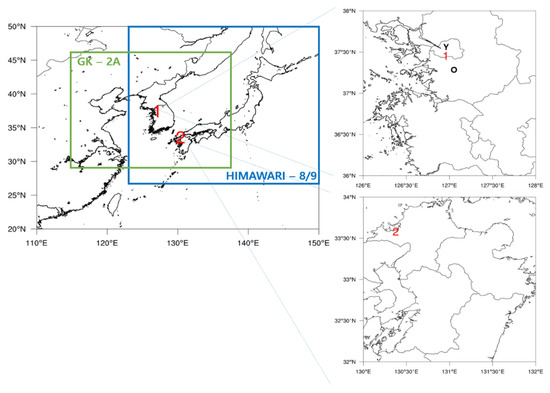
Figure 1.
The coverage of GK-2A (green box) and HIMAWARI-8/9 (blue box). The mark Y, 1, O and 2 indicate the location of Yonsei University, Seoul National University (SNU) station, Osan rawinsonde site and Fukuoka (FUA) station, respectively, in the highlighted map.
2.3. HIMAWARI-8/9
The Japanese Meteorological Agency (JMA) launched HIMAWARI–8 in October 2014 and began operation in July 2015. To ensure the stability of the satellite observation system, JMA also launched HIMAWARI-9 (in November 2016) for use as a stand-by system, beginning operation from March 2017. JMA enables continuous operation of HIMAWARI-8/9 at approximately 140.7°E, covering the Far East Asian and Western Pacific regions as an alternative to the previous satellites in the GMS and MTSAT series.
For the dedicated meteorological mission, HIMAWARI-8/9 has a new payload, called Advanced HIMAWARI Imager (AHI), of a similar specification to the AMI onboard the GK-2A, the only difference being 1.3 and 2.3 μm in near infrared channels. Table 1 lists the central wavelengths and corresponding spatial resolution. The temporal resolution is also similar to GK-2A, at 10 min for the full disk and 2.5 min for the Japanese Islands. The target area of the HIMAWARI-8/9 for the Japanese Islands is illustrated together with the GK-2A domain in Figure 1, indicating that the satellite imagery from the two platforms (GK-2A and HIMAWARI-8/9) is appropriate for the evaluation of data quality regarding their outputs, in addition to modeling performance.

Table 1.
Summary of central wavelength and the corresponding resolution from GK-2A and HIMAWARI-8/9 satellites.
3. Satellite-Derived Solar Irradiance Models
3.1. UASIBS-KIER Model
The UASIBS-KIER model version 1.0 (hereafter V1) is optimized for the geostationary satellite, COMS, for the Korean Peninsula. Kim et al. [32] explored the modifications of the original UASIBS model and its performance against ground observations at instantaneous, hourly, and daily timescales. The modeling process is provided in detail in Kim et al. [22], and is briefly explained here. A precompiled look-up table is employed in this model to save computational expenditure [14,19,30]. The look-up table, representing the shortwave albedo at the top of atmosphere (TOA), was generated by the Goddard Space Flight Center Radiative Transfer Model (GSFC RTM) [39] as a function of the solar zenith angle, surface albedo, ozone, water vapor, aerosol optical depth (AOD), and cloud optical depth (COD) for the four cloud classes (i.e., high-, mid-, and low-level clouds, and cumulus clouds). The vertical profile of ozone concentration is taken from the monthly average of the climatological background datasets, summarized by Tilmes et al. [40]. The vertically integrated AOD measured at Yonsei University (Figure 1) as part of the AErosol RObotic NEwork (AERONET) station is redistributed at each vertical level by using an exponential distribution to parameterize the extinction coefficient of aerosols, which is employed in the reduction of solar irradiance due to aerosol itself in the GSFC RTM [41]. The water vapor profile is obtained from a rawinsonde launched from Osan station (Figure 1) at 1200 UTC (2100 KST = UTC + 9) on the day before the proposed date.
After creating the look-up table, cloud detection for optically thick clouds is achieved by using brightness temperatures at the infrared and shortwave infrared channels for coarse resolution [42]. To detect optically thin or small cloud patches within coarse grid cells, we use the difference between the shortwave TOA albedo and the clear sky composite shortwave albedo that is determined as a minimum value of visible reflectance for the previous 15 days [19]. Using the clear sky composite albedo (Amin) and its standard deviation (σmin), the currently observed shortwave TOA albedo (A1) for fine resolution in each target area is classified as being clear, obscure or overcast, according to the following criteria:
Clear pixel: A1 < Ath,
Obscure pixel: Ath ≤ A1 ≤ 0.35
Overcast pixel: A1 > 0.35
where Ath is the threshold value for clear pixel. The shortwave TOA albedo overcast threshold value of 0.35 is taken from the study of Pinker et al. [19]. Following the classification of each pixel in the target area, the number of pixels in each class is counted. The obscure pixel count is redistributed into clear and overcast counts, by weighting the number of obscure pixels by the mean shortwave TOA albedo of the obscure pixels, according to the following procedure:
Above Aobscure is the mean shortwave TOA albedo of the obscure pixels in each target area.
After cloud detection, classification of cloud type is then performed using the cloud top pressure (CTP) and the shortwave TOA albedo as follows: high-level cloud (50 ≤ CTP < 440 hPa and shortwave TOA albedo < 0.6); mid-level cloud (440 ≤ CTP < 680 hPa); low-level cloud (680 ≤ CTP < 1000 hPa); and cumulus cloud (50 ≤ CTP < 440 hPa and shortwave TOA albedo ≥ 0.6). The atmospheric transmittance is obtained by comparing the shortwave TOA albedo between the satellite observation and the look-up table at the given conditions of the cloud class, solar zenith angle, and surface albedo. Finally, solar irradiance on the ground surface is calculated by multiplying the cloud fraction, atmospheric transmittance, and time-varying extraterrestrial solar irradiance that is corrected by the equation of time and the Sun-Earth distance.
The National Meteorological Satellite Center (NMSC), as a part of the KMA, provides the COMS Level-1B at visible and four different infrared channels. For the UASIBS–KIER model V1, the visible reflectance at 0.67 μm and brightness temperatures at the shortwave infrared channel (3.7 μm), and the infrared channel (10.8 μm) in wavelengths, are employed to distinguish between the clear and cloudy pixels. The downwelling surface shortwave radiation is then derived through physical modeling. Solar irradiance from the GK-2A Level-1B output is derived in a similar manner to the UASIBS-KIER model version 1.0. Visible reflectance is taken at 0.64 μm, and brightness temperature at infrared and shortwave infrared channels is taken from 10.4 and 3.9 μm, respectively. The UASIBS-KIER model for the GK-2A is named version 2.0 (hereafter V2). The only difference between version 1.0 and 2.0 is the spatial and temporal resolution (1 km vs. 0.5 km). Image quality at 0.5 km resolution is more improved than that at 1 km, and therefore the classification of clear, obscure and overcast pixels is more clarified when visible reflectance at 0.5 km is employed in the UASIBS-KIER model V2 with the GK-2A. Since the spatial resolution is 500 m at 0.64 μm in the central wavelength, downwelling surface shortwave radiation is produced, corresponding to visible reflectance at 0.64 μm. Therefore, the UASIBS-KIER model version 1.0 estimates the downwelling surface shortwave radiation at 1 × 1 km2 grid cells, but the updated version (2.0) can predict solar insolation at a 0.5 × 0.5 km2 grid resolution.
3.2. NMSC–INS Model
The NMSC produces three types of shortwave radiation data [43]; (1) shortwave radiation at the TOA; (2) downwelling surface shortwave radiation; and (3) absorbed surface shortwave radiation. The broadband albedo at the TOA is formulated by six reflectance values from channel 1 to 6 (shown in Table 1). Atmospheric transmittance is then parameterized based on the regression model as a function of the broadband albedo at the TOA at the level of longitude, latitude, vegetation, solar zenith angle, satellite zenith angle, relative azimuth, and cloud detection. In the NMSC–INS model, the Santa Barbara DISTORT Atmospheric Radiative Transfer model is employed to generate the regression model. The NMSC operates the NMSC–INS model during daytime, which means that both the solar zenith angle and the satellite zenith angle are lower than 70°. Temporal resolution is the same as the UASIBS–KIER model version 2.0, but spatial resolution is 2 km, which is four times coarser than the UASIBS–KIER model.
3.3. JAXA–INS Model
The Japanese Aerospace eXploration Agency (JAXA) Earth Observational Research Center has distributed the HIMAWARI-8/9 Level-2 datasets using Level-1 data provided by the JMA through the P-Tree system (https://www.eorc.jaxa.jp/ptree/index.html). JAXA produces data for shortwave surface radiation and photosynthetically available radiation (PAR) for the region (24–50°N, 123–150°E), including the Japanese Islands and the Korean Peninsula, at a 1 km resolution. The temporal resolution differs for the timescale. Solar irradiance is estimated every 10 min at Level-2, and hourly, daily, and monthly outputs are generated for Level-3. The research of Frouin and Murakami [44] is used to derive the solar irradiance from the HIMAWARI-8/9 Level-1. The primary purpose of their study is to estimate the PAR in the spectral range from 400 to 700 nm. However, the PAR model in their study can be extended to derive the downwelling surface shortwave radiation in the algorithm.
Frouin and Murakami [44] assumes the plane-parallel atmosphere and decoupling between clear and cloudy skies. In their study, clear sky solar irradiance is defined with the assumption of a non-reflecting surface:
where θs and S0 are solar zenith angle and solar constant, respectively; Td is the clear sky transmittance for diffused components; and Tg is the gaseous transmittance for Rayleigh scattering. Incoming solar irradiance is more diminished by the extinction of irradiance due to cloud or ice particles passing through the cloud layer. Consequently, solar irradiance in the cloudy sky is more complicated to parameterize:
Here, As is the ground surface albedo; and Sa and A are the spherical and cloud/ice albedo, respectively. The transmittance and albedo values are formulated in detail in Frouin and Murakami [44]. The evaluation of their PAR estimates against Sea-viewing Wide Field-of-View Sensor (Sea WiFS) estimates showed that the relative Root Mean Square Error (RMSE) are 22, 13, and 8% for daily, weekly, and monthly time scales, respectively.
4. Data and Error Metrics
4.1. Research Area and Ground Observations
The research area is limited to the Korean Peninsula (32–44°N, 124–132°E) and part of the Japanese Islands (Figure 1), except the UASIBS-KIER model V1, which was operated over the South Korea (32–48°N, 124–130°E). This study uses in situ measurements from the Seoul National University station, operated by KIER and Fukuoka station as a part of the Baseline Surface Radiation Network (BSRN). BSRN is a component project of the Global Energy and Water Cycle Experiment (GEWEX), operating under the aegis of the World Climate Research Programme (WCRP), to evaluate satellite derived solar irradiance [45]. The geographic details are listed in Table 2, which introduces global horizontal irradiance (GHI), direct normal irradiance (DNI), and diffuse horizontal irradiance (DHI) measured by pyranometer and pyrheliometer at all stations. FUA station is out of domain from the UASIBS-KIER model V1 and therefore quantitative analysis for the UASIBS-KIER model V1 is not made at FUA station. Data quality control is conducted before the evaluation according to the criteria presented in Gueymard and Ruiz-Arias [46].
Table 2.
Summary of geographical details for each station with observed variables. The full title of measurements is explained in the main text.
The data points are accepted when all following conditions are satisfied:
Here, h is the terrain height listed in Table 2 and S0n is the extraterrestrial irradiance on a normal surface. In a given condition (a), Gueymard and Ruiz-Arias [46] set the threshold value for θs as 85°. However, we reduced the threshold value to 75°, because the solar irradiance measured at low sun elevations is occasionally contaminated by solar reflection and beam blocking due to the surrounding buildings at the SNU station [47]. Measurements are made each minute, which is sufficient for the validation of the instantaneous estimates. Measurements are then averaged into hourly and further daily mean solar irradiance. The investigation period covered 1 October to 31 December 2019.
4.2. Error Metrics
The GHI estimates are evaluated against the ground observation stations for the instantaneous time scale. For the sake of simplicity, this study defines the observed (ktm) and modeled (ktf) clear sky indices as follows:
where GHIo, GHIe, and GHIc indicate the observed GHI, the estimated GHI, and the estimated clear sky GHI, respectively. The primary error metrics for GHI estimations are the determination coefficient (γ2), Mean Bias Error (MBE) (Equation (9)), and the Root Mean Square Error (RMSE) (Equation (10)). The secondary error metrics for comparative modeling performance between all of the models are the relative MBE (rMBE) (Equation (11)) and the relative RMSE (rRMSE) (Equation (12)):
Relative error metrics as a percentage of maximum total irradiance are already introduced in Mathiesen et al. [48], and more recently in Bueso et al. [49], to validate the variability from the clear sky irradiance. These error metrics are compared quantitatively, regardless of changes in maximum irradiance due to the solar diurnal variation, geographic position, and time of year.
5. Results
5.1. Instantaneous Evaluation
DHI is sometimes much higher than GHI at an instantaneous timescale, which is referred to as overirradiance or cloud enhancement [50,51,52]. This is due to the reflection of solar radiation at the edges of clouds. This study eliminates pairs of estimates and observations from the analysis when the ktm is higher than 1.1 to avoid the overirradiance. The GHI measured by pyranometer is averaged over 10 min intervals centered on the acquisition time of the satellite imagery provided by COMS, GK-2A, HIMAWARI-8/9, for comparison with the GHI estimates, because the COMS MI sensor takes 27 min to scan the entire field of view of the target area. Previous studies [22,32] separately validated the instantaneous GHI estimates for clear and cloudy skies. Therefore, this study also follows the same threshold value of ktm, as described in Kim et al. [22]. The clear sky is determined when ktm > 0.9, otherwise, the cloudy sky is determined.
Two examples of the instantaneous GHI estimates are provided in Figure 2 with ground observations at the SNU and FUA stations. The behavior of GHI estimates are approximately similar between V1 and V2 of the UASIBS-KIER model. This makes sense because the look-up table for the clear sky is generated by GSFC RTM with the same ancillary data (AOD, O3 and water vapor profiles), regardless of the UASIBS-KIER model version. The JAXA-INS model estimates that the GHI is larger than observed in the SNU station. In the study of Frouin and Murakami [44], clear sky GHI is dependent itself on clear sky transmittance. Uncertainties of AOD appear to influence the large deviation from ground data at the SNU station. Additionally, the NMSC-INS model produces a negative bias at noon, which means that the GHI is attenuated due to the clouds. However, the infrared image at 10.5 μm shows that there are no clouds near the SNU area at 1200 KST of 11 October 2019. The NMSC-INS model is also consistent with the clear sky (Figure 3b). Underestimation of GHI implies that the NMSC-INS model has a critical issue in the estimation of clear sky GHI in the middle of the day. Moreover, all models produce the clear sky or generate higher values of GHI estimates near the SNU station, whereas only the UASIBS-KIER model detects optically thick cloud bands in the southwest of the SNU station (see Figure 3a for reduced GHI values over the C area, compared with the clear sky GHI). The NMSC–INS model estimates the reduced GHI, but it does not result directly from the extinction due to cloud droplets. In Figure 3c, there are several pixels where the GHI is lower than 620 W·m−2 when the sky is clear. This appears to be associated with the surface albedo. More detail is provided in the following discussion section.
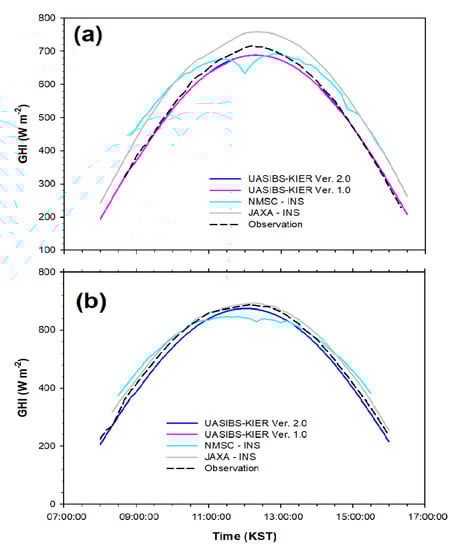
Figure 2.
Instantaneous GHI observations (dashed line) and estimates from the UASBIS-KIER model V2 (blue), V1 (magenta), the NMSC-INS model (light blue) and the JAXA-INS model (grey) in 11 October 2019 at the SNU station (a) and in 31 October 2019 at the FUA station (b) for the clear sky as a function of the Korean Standard Time.
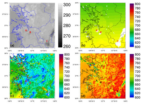
Figure 3.
Horizontal distribution of (a) brightness temperature (K) at 10.5 μm and GHI estimates (W·m−2) at 1200 KST of 11 October 2019 over the SNU station from (b) UASIBS-KIER model V2, (c) NMSC-INS model, and (d) JAXA-INS model. The mark X is the location of SNU station. A, B, C regions indicate the cloudy pixels in each panel.
As illustrated in Figure 2b, a similar behavior of the NMSC-INS model is seen in FUA, with estimated GHI lower than that observed at noon. Contrastingly, GHI is overestimated when sun elevation is low at both stations. Contrary to the NMSC-INS model, other estimates from the UASIBS–KIER and JAXA-INS models are consistent with the observed GHI. Therefore, the retrieval process needs to be fixed for it to be improved for the NMSC-INS model to capture the GHI when the sky is clear (Figure 4).
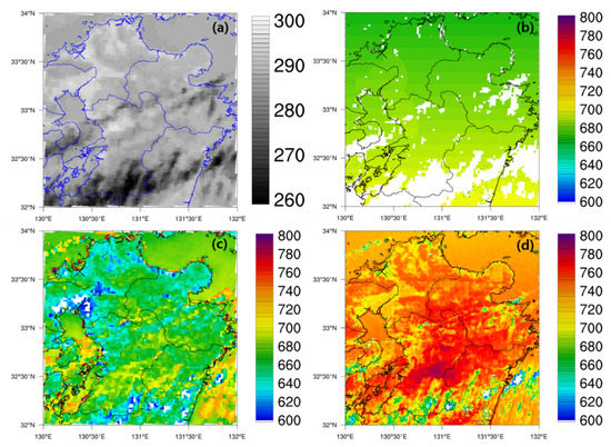
Figure 4.
Horizontal distribution of (a) brightness temperature (K) at 10.5 μm and GHI estimates (W·m−2) at 1200 KST of 31 October 2019 over the FUA station from (b) UASIBS-KIER model V2, (c) NMSC-INS model and (d) JAXA-INS model. The mark X is the location of FUA station.
The time series of GHI estimates in the cloudy skies is provided in Figure 5, which shows that the UASIBS-KIER model V2 estimates the GHI that is most consistent with the observed GHI. Despite the similar behavior of GHI estimates between V1 and V2 of the UASIBS-KIER model, the previous version overestimates the GHI when compared to observations at the SNU station. The JAXA-INS model estimates the cloudy sky GHI in the morning and then clear sky GHI in the afternoon. However, there are positive biases for the all-day data. This is mirrored in Figure 2, which means that the uncertainties of AOD, in addition to the water vapor mixing ratio, creates the large bias at the SNU station. At 1000 KST of 14 October 2019, the NMSC-INS model does not predict the cloudy sky GHI estimates even if the cloudy sky GHI is observed at the SNU station. This is due to the failure of cloud detection. As illustrated in Figure 6, the brightness temperature at 10.5 μm implies that cloud layer covers the sky over the SNU station. The direct comparison of the UASIBS-KIER and NMSC-INS models reveals a distinct difference in the cloud fraction. The finer spatial resolution of the UASIBS-KIER model enables the description of cloud microphysical characteristics to a greater extent than the NMSC-INS model. This is the case when comparing the spatial resolution between the UASIBS-KIER model V2 and the NMSC-INS model. The coarse resolution of the NMSC-INS model appears to fail to detect the cloud system at the SNU station. The JAXA-INS model employs cloudy sky data when deriving the GHI. The cloudy sky GHI at FUA is estimated by all models (Figure 7), and the best performance is found with the UASIBS-KIER model V2 (Figure 5b). However, the NMSC-INS model performed worse in any given example. Consequently, the dual detection system of cloud pixels is the major difference between the UASIBS-KIER model and the other derivation models. We will discuss the detection procedure for small clouds in the following section.
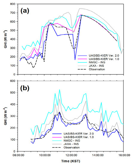
Figure 5.
Instantaneous GHI observations (dashed line) and estimates from the UASBIS-KIER model V2 (blue), V1 (magenta), the NMSC-INS model (light blue) and the JAXA-INS model (grey) on 14 October 2019 at the SNU station (a) and on 1 October 2019 at the FUA station (b) for the cloudy sky as a function of the Korean Standard Time.
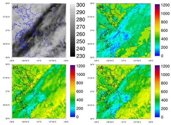
Figure 6.
Horizontal distribution of (a) brightness temperature (K) at 10.5 μm and GHI estimates (W·m−2) at 1000 KST of 14 October 2019 over the SNU station from (b) UASIBS-KIER model V2, (c) NMSC-INS model and (d) JAXA-INS model. The mark X is the location of the SNU station.
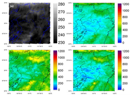
Figure 7.
Horizontal distribution of (a) brightness temperature (K) at 10.5 μm and GHI estimates (W·m−2) at 1200 KST of 1 October 2019 over the FUA station from (b) UASIBS-KIER model V2, (c) NMSC-INS model and (d) JAXA-INS model. The mark X is the location of the FUA station.
Figure 8 shows scatter plots of all sky GHI estimates together with GHI measurements at the SNU station during the investigation period. All estimates from all models (except NMSC-INS) are highly correlated with the observations: γ2 = 0.93 for the UASIBS-KIER model V1; γ2 = 0.90 for the UASIBS-KIER model V2; γ2 = 0.82 for the NMSC-INS model; and γ2 = 0.89 for the JAXA-INS model. In Figure 8b,c, NMSC-INS and JAXA-INS models generate cloudy sky GHI estimates that are positively biased for the GHI measured lower than 500 W·m−2, resulting in a larger intercept than the UASIBS-KIER model series. The dispersion of GHI pairs is smaller when sky is determined to be clear. This is understandable, as it is more complicated to parameterize the extinction of solar irradiance owing to cloud droplets or ice particles [53,54,55,56]. Furthermore, there are fewer deviations from the clear sky GHI in the UASIBS-KIER model series when compared to other models (i.e., NMSC-INS and JAXA-INS). The negative biases of clear sky GHI identified in Figure 8c,d might be due to the difference of spatial resolution that results in a failure to determine the clear sky. This will be discussed in greater detail in Section 6. The characteristics of biases for the GHI estimates from all derivation models are also found in the FUA station (see Figure 9).
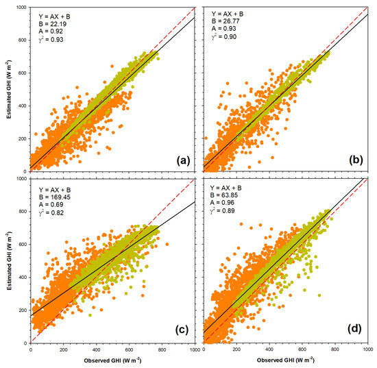
Figure 8.
Scatter plot of the instantaneous GHI observations and estimations from the UASIBS-KIER model V2 (a), V1 (b), the NMSC-INS model (c), and the JAXA-INS model (d) at the SNU station. The slope and intercept of linear regression is given together with the determination coefficient in each panel. Red dashed line indicates the reference regression.
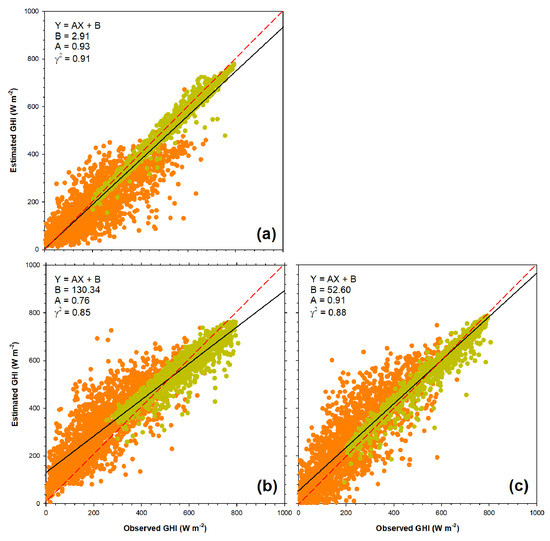
Figure 9.
Scatter plot of the instantaneous GHI observations and estimations from the UASIBS-KIER model V2 (a), the NMSC-INS model (b), and the JAXA-INS model (c) at the FUA station. The slope and intercept of linear regression is given together with the determination coefficient in each panel. Red dashed line indicates the reference regression.
The error statistics at instantaneous GHI estimates are summarized in Table 3 and Table 4 for the SNU and FUA stations, respectively. The MBE between the instantaneous estimates and observations is −3.1 W·m−2 for the UASIBS-KIER model V2 (shown in Figure 8). For the clear sky GHI estimates, the rRMSE values are very similar for the series of the UASIBS-KIER model: 4.8% for V2 and 4.6% for V1. Contrastingly to the UASIBS-KIER model, on average, the NMSC-INS model produces the clear sky GHI with a rRMSE of 12.8%, which is attributed to the large dispersion of clear sky GHI estimations in Figure 8b. Similarly, the rRMSE from the JAXA-INS model is 12.9%. However, rMBE in the JAXA-INS model is two-times larger than that of the NMSC-INS model: 9.2% for the JAXA-INS model, but 4.4% for the NMSC-INS model. Higher bias might imply that bias correction could improve the error statistics. For example, Kim et al. [57] found the correction factor as a function of solar zenith angle and then improved the results. In addition, the approximate GHI estimates are positively biased against the ground observations at the SNU stations (as shown in Figure 8d). Consequently, the JAXA-INS model could be referred to as being a better model than the NMSC-INS model if it were to be corrected.
Table 3.
Error statistics of instantaneous GHI estimations from all models during the investigation period at the SNU station. The ‘n’ is number of samples.
Table 4.
Error statistics of instantaneous GHI estimations from all models during the investigation period at the FUA station. The ‘n’ is number of samples.
The rRMSE values at cloudy sky are higher those at clear sky, which means that the relationship between cloud microphysics and the radiative transfer process is still complicated. After updating the UASIBS-KIER model to V2, the rRMSE is reduced from 19.2% to 14.5% at the SNU station. Even if the NMSC-INS model employs the same images as the UASIBS-KIER model, the modelling performance is quite different between the two models. For the UASIBS-KIER model V2 and NMSC-INS models, rRMSE values are 14.5% and 27.3%, respectively. The rRMSE value is far higher in the NMSC-INS model than in the previous version of the UASIBS-KIER model. It appears that a simple regression model, which is used in the NMSC–INS model, has the limitation to parameterize either transmittance or extinction of solar irradiance.
The behavior of error statistics is similar between the two observation stations (SNU and FUA) (Table 4). The most effective model is the UASIBS-KIER model V2 for both clear and cloudy sky. The JAXA-INS model shows better results at the FUA station than the SNU station: MBE is only 5.1 W·m−2. This is attributable to optimized transmittance based on local meteorological characteristics in Japan. In a similar manner, the UASIBS-KIER model V2 performs worse at the FUA station than the SNU station with the rRMSE raised to 13.1% for all sky conditions. A previous study made by Damiani et al. [34], who derived solar irradiance by using HIMAWARI-8/9 and Comprehensive Analysis Program for Cloud Optical Measurement algorithm, showed that the RMSE values for the instantaneous GHI observations ranged from 79 to 105 W·m−2 for Chiba, Fukue, Hedo, Miyako in Japan in 2016.
5.2. Hourly Evaluation
The comparison of hourly mean GHI estimations with observations is conducted by averaging the instantaneous pairs for each hour at two ground stations. Figure 10 shows the scatter plots of the GHI, estimated by four derivation models and measurements at the SNU station every hour. The determination coefficients of linear regressions are all higher than 0.90. In general, error statistics improve with the timescale due to the offset of biases while averaging. The research series of Kim et al. [22,32,58] showed that the RMSE was reduced as timescale increased. The slope of linear regression in the NMSC-INS model is 0.74, implying positive biases for the lower GHI observations (Figure 10c). As accounted for in the previous section, the JAXA-INS model estimates solar irradiance that is positively biased for all hours. Similar characteristics are also found in the FUA station, as illustrated in Figure 11. The positive biases produced by the JAXA-INS model are eliminated at the FUA station.
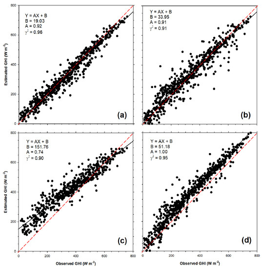
Figure 10.
Scatter plot of the hourly mean GHI observations and estimations from the UASIBS-KIER model V2 (a), V1 (b), the NMSC-INS model (c) and the JAXA-INS model (d) at the SNU station. The slope and intercept of linear regression is given together with the determination coefficient in each panel. Red dashed line indicates the reference regression.
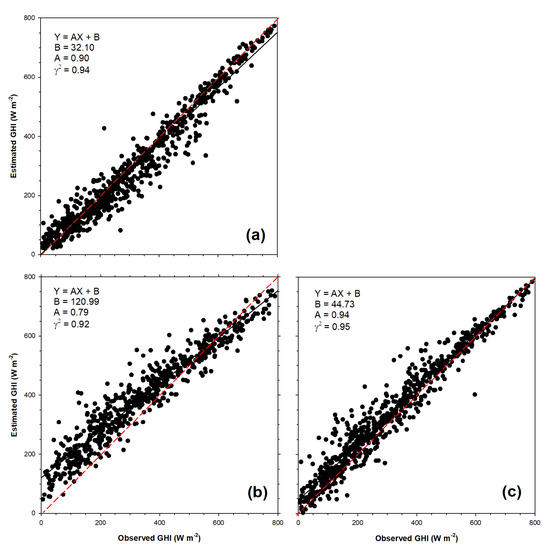
Figure 11.
Scatter plot of the hourly mean GHI observations and estimations from the UASIBS-KIER model V2 (a), the NMSC-INS model (b) and the JAXA-INS model (c) at the FUA station. The slope and intercept of linear regression is given together with the determination coefficient in each panel. Red dashed line indicates the reference regression.
Table 5 summarizes the error statistics for hourly GHI estimates at the SNU and FUA stations. The UASIBS-KIER model V2 only produces the negative biases on averages. The largest rRMSE values are found in the NMSC-INS model at all stations: 20.4% at SNU station and 18.3% at the FUA station. The hourly mean or total GHI is useful for the estimation of solar power generation from photovoltaic systems because variability in solar irradiance is a prominent barrier to the extending of renewable energy. The nominal RMSE, which is defined as the ratio of RMSE to maximum solar irradiance, is widely used in energy research [49]. Assuming that the maximum solar irradiance is 800 W·m−2 during the investigation period, the nominal RMSE values are 4.8%, 7.4%, 12.1%, and 9.8%, for the UASIBS-KIER model V1, V2, NMSC-INS, and JAXA-INS models, respectively. The Korea Power eXchange (KPX) plans to offer an incentive to renewable energy providers who accomplish the reliable daily forecast of solar power generation. The threshold value of the nominal RMSE is 10% for the day ahead of forecast [59]. The nominal RMSE of the NMSC-INS model is higher than the threshold value set by KPX, even if the hourly mean GHI estimates are taken from the remote sensing outputs. In contrast, the UASIBS-KIER model V2 generates the lowest rRMSE at the two stations. In comparison with the previous studies, Letu et al. [36] evaluated the JAXA-INS model against ground observations operated by Chinese Meteorological Administration (CMA) and then mentioned that average of RMSE values is 101.86 W·m−2 for 33 CMA stations in 2016. More recently, Peng et al. [37] improved modeling performance through the artificial neural network to derive the solar irradiance from the HIMAWARI-8/9 over China. In their study, RMSE values were 88.86 W·m−2 for the hourly time scale.
Table 5.
Error statistics of hourly mean GHI estimates from all models during the investigation period.
5.3. Daily Evaluation
The daily GHI aggregates are determined by the integration of hourly accumulations from the in situ measurements and estimations for any given day. The scatter plots shown in Figure 12 and Figure 13 indicate that the daily mean GHI estimates from the UASIBS-KIER model series are in good agreement with the observed GHI values. However, the NMSC-INS and JAXA-INS models are biased in a similar manner to the hourly mean GHI estimates. Table 6 lists the negative MBE averages that were produced by the UASIBS-KIER model V2 for all individual ground stations. The rMBE averages are −0.66% and −4.0%, which correspond to −3.0 W·m−2 and −19.7 W·m−2 at the SNU and FUA stations, respectively. Negative biases are observable for the daily accumulated GHI in other studies [60,61,62]. For example, Baek et al. [60] showed that the MBE for daily mean estimations are −28.47 W·m−2 and −25.51 W·m−2 at two different flux towers.
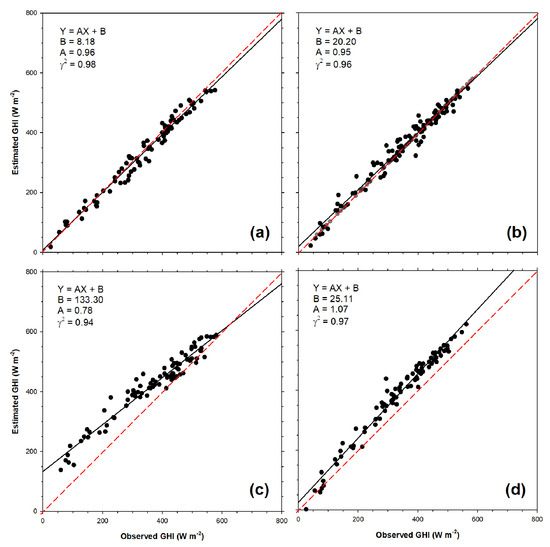
Figure 12.
Scatter plot of the daily mean GHI observations and estimations from the UASIBS-KIER model V2 (a), V1 (b), the NMSC-INS model (c) and the JAXA-INS model (d) at the SNU station. The slope and intercept of linear regression is given together with the determination coefficient in each panel. Red dashed line indicates the reference regression.
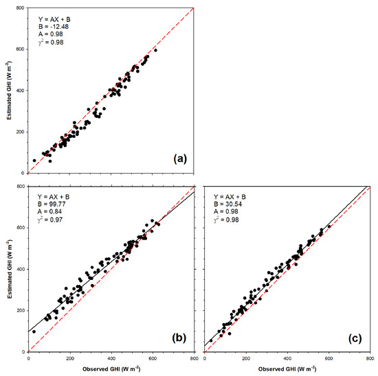
Figure 13.
Scatter plot of the daily mean GHI observations and estimations from the UASIBS-KIER model V2 (a), the NMSC-INS model (b) and the JAXA-INS model (c) at the FUA station. The slope and intercept of linear regression is given together with the determination coefficient in each panel. Red dashed line indicates the reference regression.
Table 6.
Error statistics of daily mean GHI estimates from all models during the investigation period.
For all of the individual stations, the UASIBS-KIER model V2 yields the most reliable estimates: 4.5% at the SNU station and 6.0% at the FUA station. In contrast, the direct comparison between the two models shows that the NMSC-INS model has a limitation when estimating the solar insolation on the ground because the rRMSE values exceed 10% for all stations (Table 6). Therefore, the daily aggregates from the UASIBS-KIER model V2 can be employed to build the solar resource map.
6. Discussion
The quantitative evaluation of the GHI estimates against the observations for the different time scales indicates that the UASIBS-KIER model with fine spatial resolution performs better than that with coarse resolution. We will now discuss the effects of horizontal resolution on the performance of modeling when deriving solar irradiance. As illustrated in Figure 6, the failure of cloud detection for small clouds or cloud edges leads to critical problems, resulting in a large deviation of the GHI estimated by the models. The contingency tables for both clear and cloudy skies at the SNU and FUA stations are provided in Table 7. The classification of clear sky is one of a set of possible events that may happen, which means that it is categorized as a “yes/no” forecast or estimate, i.e., the event will or will not occur. The threshold values for a clear sky are 0.9 of ktm and ktf for the observation and estimates, respectively (a clear sky is recognized when ktm > 0.9).
Table 7.
Contingency table of the clear sky detection by all models at the SNU station.
When the sky is observed as being cloudy, models sometimes determine the pixels as clear sky. To clarify the performance of cloud detection, we list the hit rate (HR) and false alarm rate (FAR) for the clear sky in Table 8. HR is defined as the simple fraction of the estimated event, whereas FAR is that proportion of estimated events that fail to happen. On average, the HR value of the NMSC-INS model is the lowest. However, the opposite is true for the UASIBS-KIER model V2, in which HR is higher than 0.98 at the SNU station. When updating the UASIBS-KIER model to V2 with the new satellite platform, HR increases but FAR decreases. The lowest FAR is found in the UASIBS-KIER model V2 in both stations, which means that this model is the most reliable. The direct comparison of the NMSC-INS and JAXA-INS models shows that the FAR values are similar, but the NMSC-INS model estimates the GHI with an rRMSE higher than the JAXA-INS model. This means that there is no large discrepancy for the detection of cloud pixels between the two models, but the JAXA-INS model formulates the extinction of incoming solar irradiance more elaborately.
Table 8.
Summary of Hit Rate and False Alarm Rate (FAR) estimated by all models for the clear sky at the SNU station.
Compared to the clear sky, the NMSC-INS model estimates the lower GHI during the middle of day, compared to the clear sky GHI (see Figure 2). The time series of GHI estimates at the instantaneous timescale, averaged over three months from October to December 2019, are shown in Figure 14. In a similar manner to a single example (Figure 2), the products from the UASIBS-KIER models agree with the GHI averages measured at the SNU station. However, the JAXA-INS model generates positive biases against the ground observation. At the FUA station, the opposite is true for the JAXA-INS model, which shows good agreement with the observation for the JAXA-INS model. Even in clear sky, the NMSC-INS model generates the lower GHI estimations during the day, but positive biases are seen at low sun elevations. Figure 3 shows the horizontal distribution of GHI estimates near SNU station. Unlike the other models, only the NMSC-INS model does not show homogeneous GHI distribution for the clear sky pixels. This can be attributed to the formulation of downwelling surface shortwave radiation as a function of surface albedo in the NMSC-INS model [43]. The extension of GHI distributions into the Korean Peninsula also indicates that the GHI estimates are lower in the NMSC-INS model than in the other models over the northern part of the Korean Peninsula, even when sky is clear. This is because the surface albedo plays a role in reducing incoming solar irradiance (Figure 15).
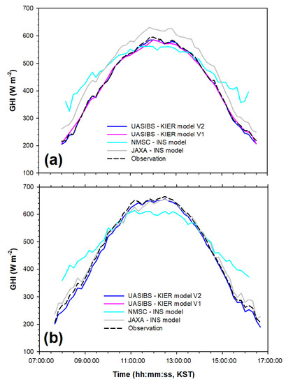
Figure 14.
Time series of instantaneous GHI observations (dashed line) and estimates from the UASIBS-KIER model V2 (blue), V1 (magenta), the NMSC-INS model (light blue) and the JAXA-INS model (grey) averaged over the investigation period from October to December 2019 at the SNU (a) and FUA (b) station.
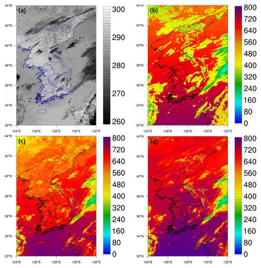
Figure 15.
Horizontal distribution of (a) brightness temperature (K) at 10.5 μm and GHI estimates (W·m−2) at 1200 KST of 11 October 2019 over the Korean Peninsula from (b) UASIBS-KIER model V2, (c) NMSC-INS model and (d) JAXA-INS model.
The discussion now addresses the difference in the number of samples between the NMSC-INS model and the UASIBS-KIER model V2. Table 2 lists the missing data as 156 and 338 for the clear and cloudy skies, respectively, when compared to the UASIBS-KIER model V2. Figure 16 shows the frequency distribution of missing data for the solar zenith angle. Most of the missing data occurred in the 70–80° bin, which is understandable due to the NMSC-INS model, which only operates when the solar zenith angle is lower than 70°. Nevertheless, there remains 66 missing data counts in the cloudy sky for the solar zenith angle lower than 70°. These missing data are due to the treatment of Not a Number for the deep cloud layer. Figure 17 is evidence for the Not a Number problem when deep cloud layer exists. Cloud bands pass through the Korean Peninsula, but solar irradiance is not retrieved at some pixels. More recently, RGB true color imagery shows that the deep cloud system is located over the northern part of the Korean Peninsula. However, GHI estimations are not made over these cloud pixels. Therefore, the NMSC-INS model has a critical limitation in building the solar resource map for the resource assessment.
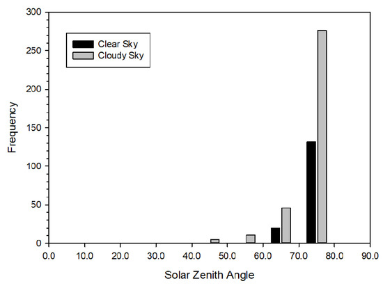
Figure 16.
Frequency distribution of solar zenith angle at clear (black) and cloudy (grey) sky from the missing data of UASIBS-KIER model V1 at the SNU station.
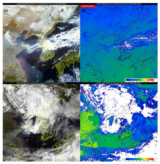
Figure 17.
True color image (a,c) and GHI distribution (b,d) from the NMSC-INS model; (a,b) at 1220 KST of November 15, 2019, (c,d) at 1540 KST of 22 May 2020 (taken from http://nmsc.kma.go.kr/homepage/html/satellite/viewer/selectSatViewer.do?dataType=operSat).
7. Conclusions
The new satellite platform, GK-2A, was launched by the Korea Meteorological Administration on 5 December 2018, to replace the official operation of the COMS. The GK-2A includes the AMI sensor, which has a spectral range similar to the AHI included in HIMAWARI-8/9. The UASIBS-KIER model for deriving the downwelling surface shortwave radiation was updated to employ visible and infrared imagery from the GK-2A. The Korean Peninsula is covered by the field of view from the both GK-2A and HIMAWARI-8/9. Therefore, we can compare the satellite-derived solar irradiance between the UASIBS–KIER model with the GK-2A and the JAXA-INS model with the HIMAWARI-8/9 against instantaneous ground observations at Seoul National University, operated by the KIER and Fukuoka station as part of the BSRN from October to December, 2019. In addition, this study attempts to evaluate the NMSC-INS model that is operated by KMA, compared to UASIBS-KIER model series and JAXA-INS model.
An evaluation at the instantaneous timescale was conducted separately for the clear and cloudy skies. For the clear sky, the RMSE normalized to the clear sky GHI are recorded at the SNU station as 4.8%, 12.8%, and 12.9% for the UASIBS-KIER model V2, the NMSC-INS model, and the JAXA-INS model, respectively. When compared to the cloudy sky GHI estimates at the SNU station, the difference of modeling performance between all models becomes clearer. The lowest rRMSE value is seen at the UASIBS-KIER model V2, but the NMSC-INS model, operated by the KMA, estimates the GHI observations with the largest rRMSE. The primary difference between the UASIBS-KIER model V2 and V1 is the spatial and temporal resolution, and the data quality of the sensor itself. The rRMSE value is reduced from 19.2% to 14.5% when updating the UASIBS-KIER model because the cloud detection procedure occasionally failed to detect small cloud patches even with 1 × 1 km2 grid cells. The local meteorological conditions that are employed to derive the solar irradiance from the satellite imagery sometimes affect the modeling performance. The direct comparison of GHI estimates between the UASIBS-KIER model V2 and the JAXA-INS model provides good evidence of this effect. The error statistics of the UASIBS-KIER model V2 are worse at the SNU station than the FUA station. However, opposite is true for the JAXA-INS model. This is understandable given the vertical profiles of the water vapor mixing ratio and AOD were obtained from the in situ observations at the Korean Peninsula for the UASIBS-KIER model series. Consequently, data assimilation of the local meteorological condition over the Japanese Islands has to be considered a limitation in the operation of the UASIBS-KIER model.
When averaging the GHI estimates for the longer timescales, the error statistics appear to improve. The daily mean GHI estimates are most reliable with the lowest rRMSE values, which means they are applicable for building the solar energy resource map. Figure 18a shows the daily mean GHI estimates that are averaged for October 2019. With a fine horizontal resolution, the UASIBS-KIER model accounted for the solar resource potential by region and in detail when compared with gridded datasets such as the Clouds and the Earth’s Radiant Energy System, CERES and Modern-Era Retrospective analysis for Research and Applications, MERRA outputs [58]. The temporal resolution of collection time for the full disk for the GK-2A is 10 min, and the UASIBS-KIER model V2 would be extended towards other regions. An example is provided in Figure 18b, which shows that sufficient solar resources are available to operate the photovoltaic system in Indonesia.
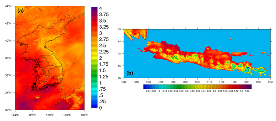
Figure 18.
Solar resource map as a result of the daily total GHI (kWh·m−2·d−1) from the UASIBS-KIER model V2 in Korea (a) and Indonesia (b) in October 2019.
Although the UASIBS-KIER model produces reliable GHI estimates, there remain limitations to employing the satellite imagery. The AMI detects the visible images at six different wavelengths to enable the generation of true color images, but we do not employ all visible channels. Therefore, we will improve the algorithm for cloud detection by using the key findings from recent research on radiative parameterization [63,64]. Furthermore, the solar irradiance derived by the satellite will also be used to forecast the GHI distributions based on the cloud motion vector.
Author Contributions
Conceptualization, methodology, validation, formal analysis and software, C.K.K.; data curation, C.-Y.Y.; Conceptualization, Y.G.L.; funding acquisition, H.-G.K.; supervision, Y.-H.K. All authors have read and agreed to the published version of the manuscript.
Funding
The APC was funded by the research and development program of the Korea Institute of Energy Research (C0-2407).
Acknowledgments
This work was conducted under framework of the research and development program of the Korea Institute of Energy Research (C0-2407).
Conflicts of Interest
The authors declare no conflict of interest.
References
- Wild, M.; Gilgen, H.; Roesch, A.; Ohmura, A.; Long, C.N.; Dutton, E.G.; Forgan, B.; Kallis, A.; Russak, V.; Tsvetkov, A. From Dimming to Brightening: Decadal Changes in Solar Radiation at Earth′s Surface. Science 2005, 308, 847–850. [Google Scholar] [CrossRef] [PubMed]
- Streets, D.G.; Wu, Y.; Chin, M. Two-Decadal Aerosol Trends as a likely Explanation of the Global Dimming/Brightening Transition. Geophys. Res. Lett. 2006, 33, L15806. [Google Scholar] [CrossRef]
- IPCC. Climate Change 2013: The Physical Science Basis. Contribution of Working Group I to the Fifth Assessment Report of the Intergovernmental Panel on Climate Change; Stocker, T.F., Qin, D., Plattner, G.-K., Tignor, M., Allen, S.K., Boschung, J., Nauels, A., Xia, Y., Bex, V., Midgley, P.M., Eds.; Cambridge University Press: Cambridge, UK; New York, NY, USA, 2013; p. 1535. [Google Scholar] [CrossRef]
- Manara, V.; Brunetti, M.; Celozzi, A.; Maugeri, M.; Sanchez-Lorenzo, A.; Wild, M. Detection of Dimming/Brightening in Italy from Homogenized All-Sky and Clear-Sky Surface Solar Radiation Records and Underlying Causes (1959–2013). Atmos. Chem. Phys. 2016, 16, 11145–11161. [Google Scholar] [CrossRef]
- Tanaka, K.; Ohmura, A.; Folini, D.; Wild, M.; Ohkawara, N. Is Global Dimming and Brightening in Japan Limited to Urban Areas? Atmos. Chem. Phys. 2016, 16, 13969–14001. [Google Scholar] [CrossRef]
- Zelenka, A.; Perez, R.; Seals, R.; Renné, D. Effective Accuracy of Satellite-Derived Hourly Irradiances. Theor. Appl. Climatol. 1999, 62, 199–207. [Google Scholar] [CrossRef]
- Vignola, F.; Harlan, P.; Perez, R.; Kmiecik, M. Analysis of Satellite Derived Beam and Global Solar Radiation Data. Sol. Energy 2007, 81, 768–772. [Google Scholar] [CrossRef]
- Chow, C.W.; Urquhart, B.; Lave, M.; Dominguez, A.; Kleissl, J.; Shields, J.; Washom, B. Intra-Hour Forecasting with a Total Sky Imager at the UC San Diego Solar Energy Testbed. Sol. Energy 2011, 85, 2881–2893. [Google Scholar] [CrossRef]
- Wegertseder, P.; Lund, P.; Mikkola, J.; García Alvarado, R. Combining Solar Resource Mapping and Energy System Integration Methods for Realistic Valuation of Urban Solar Energy Potential. Sol. Energy 2016, 135, 325–336. [Google Scholar] [CrossRef]
- Gilgen, H.; Wild, M.; Ohmura, A. Means and Trends of Shortwave Irradiance at the Surface Estimated from Global Energy Balance Archive Data. J. Clim. 1998, 11, 2042–2061. [Google Scholar] [CrossRef]
- Stanhill, G.; Cohen, S. Solar Radiation Changes in the United States during the Twentieth Century: Evidence from Sunshine Duration Measurements. J. Clim. 2005, 18, 1503–1512. [Google Scholar] [CrossRef]
- Pinker, R.T.; Ewing, J.A. Modeling Surface Solar Radiation: Model Formulation and Validation. J. Clim. Appl. Meteorol. 1985, 24, 389–401. [Google Scholar] [CrossRef]
- Rossow, W.B.; Schiffer, R.A. ISCCP Cloud Data Products. Bull. Am. Meteor. Soc. 1991, 72, 2–20. [Google Scholar] [CrossRef]
- Pinker, R.T.; Laszlo, I. Modeling Surface Solar Irradiance for Satellite Applications on a Global Scale. J. Appl. Meteor. 1992, 31, 194–211. [Google Scholar] [CrossRef]
- Li, Z.; Leighton, H.G. Global Climatologies of Solar Radiation Budgets at the Surface and in the Atmosphere from 5 years of ERBE Data. J.Geophys. Res. 1993, 98, 4919–4930. [Google Scholar] [CrossRef]
- Whitlock, C.H.; Charlock, T.P.; Staylor, W.F.; Pinker, R.T.; Laszlo, I.; Ohmura, A.; Gilgen, H.; Konzelman, T.; DiPasquale, R.C.; Moats, C.D.; et al. First Global WCRP Shortwave Surface Radiation Budget Dataset. Bull. Am. Meteor. Soc. 1995, 76, 905–922. [Google Scholar] [CrossRef]
- Zhang, Y.; Rossow, W.B.; Lacis, A.A.; Oinas, V.; Mishchenko, M.I. Calculation of Radiative Fluxes from the Surface to Top of Atmosphere Based on ISCCP and other Global Data Sets: Refinements of the Radiative Transfer Model and the Input Data. J. Geophys. Res. 2004, 109, D19105. [Google Scholar] [CrossRef]
- Gupta, S.K.; Ritchey, N.A.; Wilber, A.C.; Whitlock, C.H.; Gibson, G.G.; Stackhouse, P.W. A Climatology of Surface Radiation Budget Derived from Satellite Data. J. Clim. 1999, 12, 2691–2710. [Google Scholar] [CrossRef]
- Pinker, R.T.; Tarpley, J.D.; Laszlo, I.; Mitchell, K.E.; Houser, P.R.; Wood, E.F.; Schaake, J.C.; Robock, A.; Lohmann, D.; Cosgrove, B.A.; et al. Surface Radiation Budgets in Support of the GEWEX Continental-Scale International Project (GCIP) and the GEWEX Americas Prediction Project (GAPP), including the North American Land Data Assimilation System (NLDAS) Project. J. Geophys. Res. 2003, 108, 8844. [Google Scholar] [CrossRef]
- Wang, H.; Pinker, R.T. Shortwave Radiative Fluxes from MODIS: Model Development and Implementation. J. Geophys. Res. 2009, 114, D20201. [Google Scholar] [CrossRef]
- Ma, Y.; Pinker, R.T. Modeling Shortwave Radiative Fluxes from Satellites. J. Geophys. Res. 2012, 117, D23202. [Google Scholar] [CrossRef]
- Kim, C.K.; Holmgren, W.F.; Stovern, M.; Betterton, E.A. Toward Improved Solar Irradiance Forecasts: Derivation of Downwelling Surface Shortwave Radiation in Arizona from Satellite. Pure Appl. Geophys. 2016, 173, 2535–2553. [Google Scholar] [CrossRef]
- Gautier, C.; Diak, G.; Masse, S. A Simple Physical Model to Estimate Incident Solar Radiation at the Surface from GOES Satellite Data. J. Appl. Meteor. 1980, 19, 1005–1012. [Google Scholar] [CrossRef]
- Moser, W.; Raschke, E. Incident Solar Radiation over Europe Estimated from METEOSAT Data. J. Clim. Appl. Meteorol. 1984, 23, 166–170. [Google Scholar] [CrossRef]
- Dedieu, G.; Deschamps, P.Y.; Kerr, Y.H. Satellite Estimation of Solar Irradiance at the Surface of the Earth and of Surface Albedo Using a Physical Model Applied to Metcosat Data. J. Clim. Appl. Meteorol. 1987, 26, 79–87. [Google Scholar] [CrossRef]
- Stuhlmann, R.; Rieland, M.; Paschke, E. An Improvement of the IGMK Model to Derive Total and Diffuse Solar Radiation at the Surface from Satellite Data. J. Appl. Meteor. 1990, 29, 586–603. [Google Scholar] [CrossRef][Green Version]
- Rigollier, C.; Lefévre, M.; Wald, L. The Method Heliosat-2 for Deriving Shortwave Solar Radiation from Satellite Images. Sol. Energy 2004, 77, 159–169. [Google Scholar] [CrossRef]
- Schillings, C.; Mannstein, H.; Meyer, R. Operational Method for Deriving High Resolution Direct Normal Irradiance from Satellite Data. Sol. Energy 2004, 76, 475–484. [Google Scholar] [CrossRef]
- Geiger, B.; Meurey, C.; Lajas, D.; Franchistéguy, L.; Carrer, D.; Roujean, J.-L. Near Real-Time Provision of Downwelling Shortwave Radiation Estimates Derived from Satellite Observations. Meteor. Appl. 2008, 15, 411–420. [Google Scholar] [CrossRef]
- Ineichen, P.; Barroso, C.S.; Geiger, B.; Hollmann, R.; Marsouin, A.; Mueller, R. Satellite Application Facilities Irradiance Products: Hourly Time Step Comparison and Validation over Europe. Int. J. Remote Sens. 2009, 30, 5549–5571. [Google Scholar] [CrossRef]
- Yeom, J.-M.; Han, K.-S.; Lee, C.-S.; Kim, D.-Y. An Improved Validation Technique for the Temporal Discrepancy when Estimated Solar Surface Insolation Compare with Ground-Based Pyranometer: MTSAT-1R Data use. Korean J. Remote Sens. 2008, 24, 605–612. [Google Scholar]
- Kim, C.K.; Kim, H.-G.; Kang, Y.-H.; Yun, C.-Y. Toward Improved Solar Irradiance Forecasts: Comparison of the Global Horizontal Irradiances Derived from the COMS Satellite Imagery Over the Korean Peninsula. Pure Appl. Geophys. 2017, 174, 2773–2792. [Google Scholar] [CrossRef]
- Yeom, J.-M.; Park, S.; Chae, T.; Kim, J.-Y.; Lee, C.S. Spatial Assessment of Solar Radiation by Machine Learning and Deep Neural Network Models Using Data Provided by the COMS MI Geostationary Satellite: A Case Study in South Korea. Sensors 2019, 19, 2082. [Google Scholar] [CrossRef] [PubMed]
- Damiani, A.; Irie, H.; Horio, T.; Takamura, T.; Khatri, P.; Takenaka, H.; Nagao, T.; Nakajima, T.Y.; Cordero, R.R. Evaluation of Himawari-8 surface Downwelling Solar Radiation by Ground-Based Measurements. Atmos. Meas. Tech. 2018, 11, 2501–2521. [Google Scholar] [CrossRef]
- Shi, H.; Li, W.; Fan, X.; Zhang, J.; Hu, B.; Husi, L.; Shang, H.; Han, X.; Song, Z.; Zhang, Y.; et al. First Assessment of Surface Solar Irradiance Derived from Himawari-8 across China. Sol. Energy 2018, 174, 164–170. [Google Scholar] [CrossRef]
- Letu, H.; Yang, K.; Nakajima, T.Y.; Ishimoto, H.; Nagao, T.M.; Riedi, J.; Baran, A.J.; Ma, R.; Wang, T.; Shang, H.; et al. High-Resolution Retrieval of Cloud Microphysical Properties and Surface Solar Radiation Using Himawari-8/AHI Next-Generation Geostationary Satellite. Remote Sens. Environ. 2020, 239, 111583. [Google Scholar] [CrossRef]
- Peng, Z.; Letu, H.; Wang, T.; Shi, C.; Zhao, C.; Tana, G.; Zhao, N.; Dai, T.; Tang, R.; Shang, H.; et al. Estimation of Shortwave Solar Radiation Using the Artificial Neural Network from Himawari-8 satellite Imagery over China. J. Quant. Spectrosc. Radiat. Transf. 2020, 240, 106672. [Google Scholar] [CrossRef]
- Lorenzo, A.T.; Holmgren, W.F.; Cronin, A.D. Irradiance Forecasts Based on an Irradiance Monitoring Network, Cloud Motion, and Spatial Averaging. Sol. Energy 2015, 122, 1158–1169. [Google Scholar] [CrossRef]
- Chou, M.-D.; Suarez, M.J. A Solar Radiation Parameterization for Atmospheric Studies; 1999-104606; Goddard Space Flight Center, 1999; p. 65.
- Tilmes, S.; Lamarque, J.F.; Emmons, L.K.; Conley, A.; Schultz, M.G.; Saunois, M.; Thouret, V.; Thompson, A.M.; Oltmans, S.J.; Johnson, B.; et al. Technical Note: Ozonesonde Climatology between 1995 and 2011: Description, Evaluation and Applications. Atmos. Chem. Phys. 2012, 12, 7475–7497. [Google Scholar] [CrossRef]
- Ruiz-Arias, J.A.; Dudhia, J.; Santos-Alamillos, F.J.; Pozo-Vázquez, D. Surface Clear-Sky Shortwave Radiative Closure Intercomparisons in the Weather Research and Forecasting model. J. Geophys. Res. 2013, 118, 9901–9913. [Google Scholar] [CrossRef]
- Jedlovec, G.J.; Haines, S.L.; LaFontaine, F.J. Spatial and Temporal Varying Thresholds for Cloud Detection in GOES Imagery. Geosci. Remote Sens. IEEE Trans. 2008, 46, 1705–1717. [Google Scholar] [CrossRef]
- NMSC. A Validation Report for the Meteorological Products of GEO-KOMSAT-2A in 2018, 2018; 252.
- Frouin, R.; Murakami, H. Estimating Photosynthetically Available Radiation at the Ocean Surface from ADEOS-II Global Imager Data. J. Oceanogr. 2007, 63, 493–503. [Google Scholar] [CrossRef]
- Ohmura, A.; Dutton, E.G.; Forgan, B.; Fröhlich, C.; Gilgen, H.; Hegner, H.; Heimo, A.; König-Langlo, G.; McArthur, B.; Müller, G.; et al. Baseline Surface Radiation Network (BSRN/WCRP): New Precision Radiometry for Climate Research. Bull. Am. Meteor. Soc. 1998, 79, 2115–2136. [Google Scholar] [CrossRef]
- Gueymard, C.A.; Ruiz-Arias, J.A. Extensive Worldwide Validation and Climate Sensitivity Analysis of Direct Irradiance Predictions from 1-min Global Irradiance. Spec. Issue Prog. Sol. Energy 2016, 128, 1–30. [Google Scholar] [CrossRef]
- Kim, C.K.; Kim, H.-G.; Kang, Y.-H.; Yun, C.-Y.; Kim, S.Y. Probabilistic Prediction of Direct Normal Irradiance Derived from Global Horizontal Irradiance over the Korean Peninsula by Using Monte-Carlo Simulation. Sol. Energy 2019, 180, 63–74. [Google Scholar] [CrossRef]
- Mathiesen, P.; Collier, C.; Kleissl, J. A High-Resolution, Cloud-Assimilating Numerical Weather Prediction Model for Solar Irradiance Forecasting. Sol. Energy 2013, 92, 47–61. [Google Scholar] [CrossRef]
- Bueso, M.; Paredes-Parra, J.M.; Mateo-Aroca, A.; Molina-García, A. A Characterization of Metrics for Comparing Satellite-Based and Ground-Measured Global Horizontal Irradiance Data: A Principal Component Analysis Application. Sustainability 2020, 12, 2454. [Google Scholar] [CrossRef]
- Yordanov, G.H.; Midtgård, O.M.; Saetre, T.O.; Nielsen, H.K.; Norum, L.E. Overirradiance (Cloud Enhancement) Events at High Latitudes. IEEE J. Photovolt. 2013, 3, 271–277. [Google Scholar] [CrossRef]
- Almeida, M.P.; Zilles, R.; Lorenzo, E. Extreme Overirradiance Events in Sâo Paulo, Brazil. Sol. Energy 2014, 110, 168–173. [Google Scholar] [CrossRef]
- Piedehierro, A.A.; Antón, M.; Cazorla, A.; Alados-Arboledas, L.; Olmo, F.J. Evaluation of Enhancement Events of Total Solar Irradiance during Cloudy Conditions at Granada (Southeastern Spain). Atmos. Res. 2014, 135–136, 1–7. [Google Scholar] [CrossRef]
- Fu, Q.; Liou, K.N. Parameterization of the Radiative Properties of Cirrus Clouds. J. Atmos. Sci. 1993, 50, 2008–2025. [Google Scholar] [CrossRef]
- Ghan, S.; Wang, M.; Zhang, S.; Ferrachat, S.; Gettelman, A.; Griesfeller, J.; Kipling, Z.; Lohmann, U.; Morrison, H.; Neubauer, D.; et al. Challenges in Constraining Anthropogenic Aerosol Effects on Cloud Radiative Forcing Using Present-Day Spatiotemporal Variability. Proc. Natl. Acad. Sci. USA 2016, 113, 5804–5811. [Google Scholar] [CrossRef] [PubMed]
- Nogherotto, R.; Tompkins, A.M.; Giuliani, G.; Coppola, E.; Giorgi, F. Numerical Framework and Performance of the New Multiple-Phase Cloud Microphysics Scheme in RegCM4.5: Precipitation, Cloud Microphysics, and Cloud RadiativeEeffects. Geosci. Model Dev. 2016, 9, 2533–2547. [Google Scholar] [CrossRef]
- Thompson, G.; Tewari, M.; Ikeda, K.; Tessendorf, S.; Weeks, C.; Otkin, J.; Kong, F. Explicitly-Coupled Cloud Physics and Radiation Parameterizations and Subsequent Evaluation in WRF High-Resolution Convective Forecasts. Atmos. Res. 2016, 168, 92–104. [Google Scholar] [CrossRef]
- Kim, C.K.; Kim, H.-G.; Kang, Y.-H.; Yun, C.-Y.; Lee, S.-N. Evaluation of Global Horizontal Irradiance Derived from CLAVR-x Model and COMS Imagery Over the Korean Peninsula. New Renew. Energy 2016, 12, 13–20. [Google Scholar] [CrossRef]
- Kim, C.K.; Holmgren, W.F.; Stovern, M.; Betterton, E.A. Toward Improved Solar Irradiance Forecasts: Comparison of Downwelling Surface Shortwave Radiation in Arizona Derived from Satellite with the Gridded Datasets. Pure Appl. Geophys. 2016, 173, 2929–2943. [Google Scholar] [CrossRef]
- KPX. Guideline for the Virtual Power Plant Business. Available online: https://der.kmos.kr/sga/mainPage.do (accessed on 10 June 2020).
- Baek, J.; Byun, K.; Kim, D.; Choi, M. Assessment of Solar Insolation from COMS: Sulma and Cheongmi Watersheds. Korean J. Remote Sens. 2013, 29, 137–149. [Google Scholar] [CrossRef]
- Jee, J.-B.; Zo, I.-S.; Lee, K.-T. A Study on the Retrievals of Downward Solar Radiation at the Surface Based on the Observations from Multiple Geostationary Satellites. Korean J. Remote Sens. 2013, 29, 123–135. [Google Scholar] [CrossRef]
- Lee, J.; Choi, W.; Kim, Y.; Yun, C.; Jo, D.; Kang, Y. Estimation of Global Horizontal Insolation over the Korean Peninsula Based on COMS MI Satellite Images. Korean J. Remote Sens. 2013, 29, 151–160. [Google Scholar] [CrossRef][Green Version]
- Hong, G.; Minnis, P. Effects of Spherical Inclusions on Scattering Properties of Small Ice Cloud Particles. J. Geophys. Res. 2015, 120, 2951–2969. [Google Scholar] [CrossRef]
- Yi, B.; Yang, P.; Liu, Q.; van Delst, P.; Boukabara, S.-A.; Weng, F. Improvements on the Ice Cloud Modeling Capabilities of the Community Radiative Transfer Model. J. Geophys. Res. 2016, 121, 13577–13590. [Google Scholar] [CrossRef]


© 2020 by the authors. Licensee MDPI, Basel, Switzerland. This article is an open access article distributed under the terms and conditions of the Creative Commons Attribution (CC BY) license (http://creativecommons.org/licenses/by/4.0/).