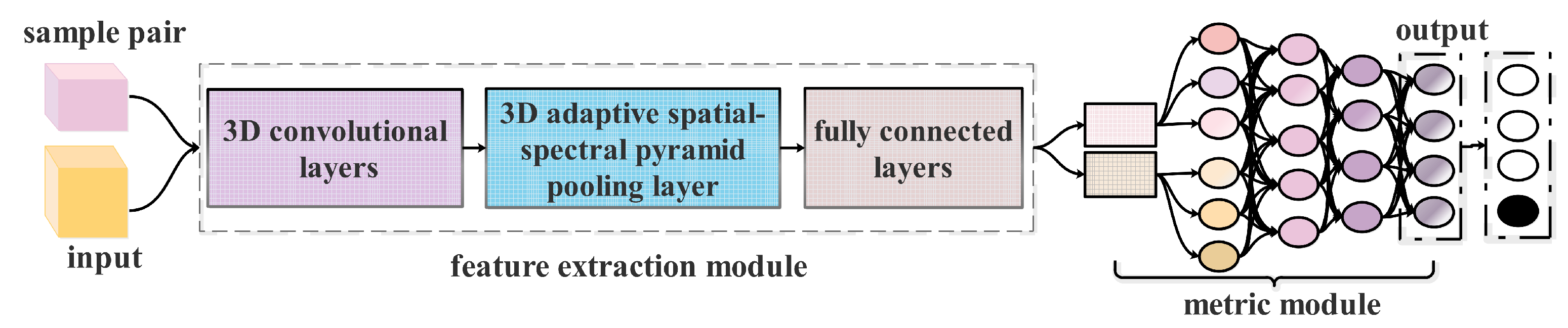
Figure 1.
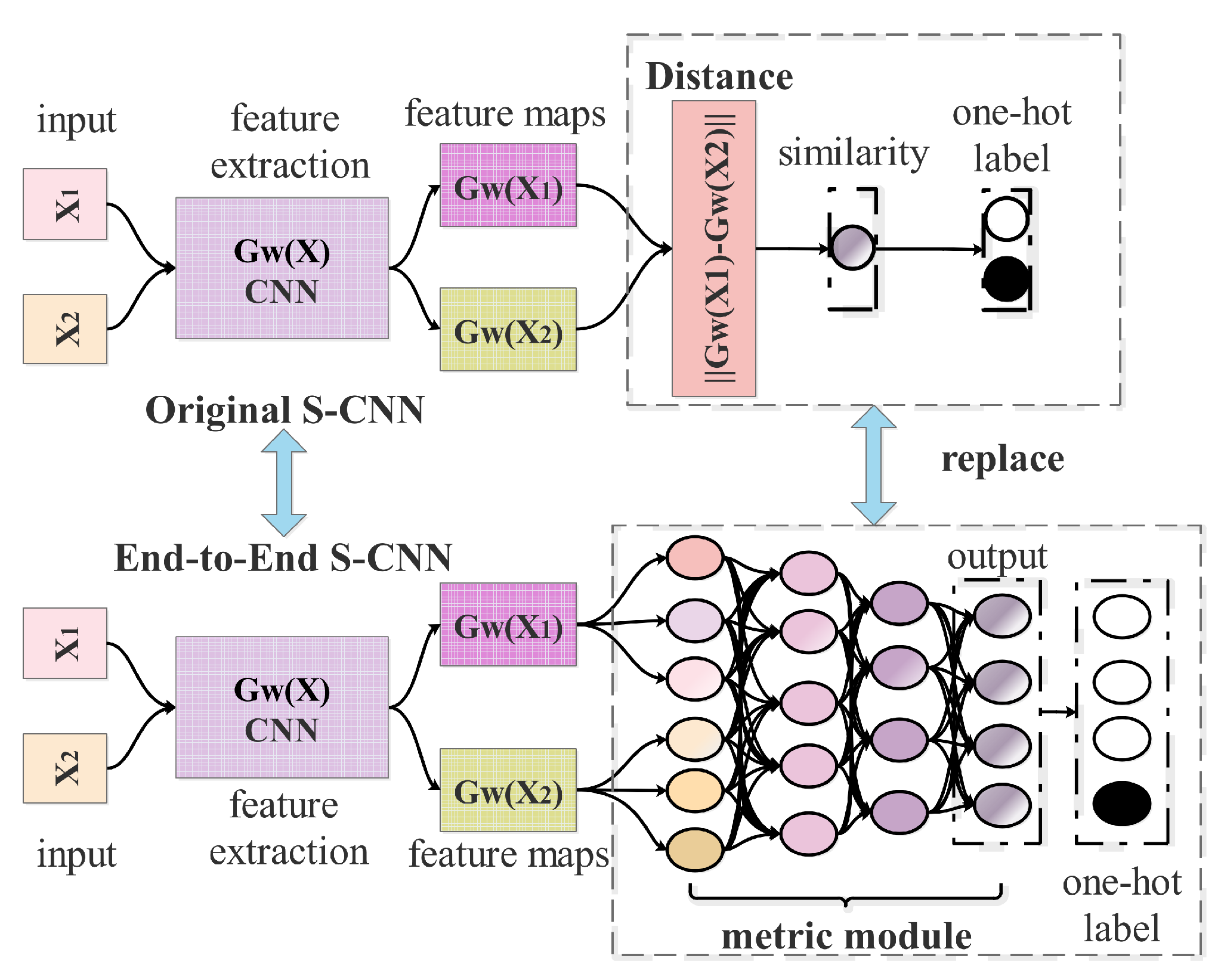
Architectures of SCNN and ES-CNN. Here the original SCNN is a binary classifier, which can learn the similarity of the input sample-pair. To deal directly with multi-classification, the ES-CNN applies a fully connected network to replace the metric function (distance) of SCNN.
Figure 1.
Architectures of SCNN and ES-CNN. Here the original SCNN is a binary classifier, which can learn the similarity of the input sample-pair. To deal directly with multi-classification, the ES-CNN applies a fully connected network to replace the metric function (distance) of SCNN.
Figure 2.
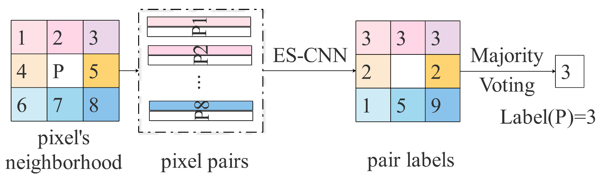
An example of voting strategy within a neighborhood.
Figure 2.
An example of voting strategy within a neighborhood.
Figure 3.
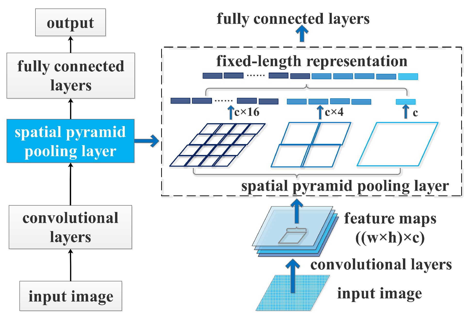
A CNN with a spatial pyramid pooling layer.
Figure 3.
A CNN with a spatial pyramid pooling layer.
Figure 4.
Architecture of a developed Siamese CNN with adaptive spatial-spectral pyramid pooling.
Figure 4.
Architecture of a developed Siamese CNN with adaptive spatial-spectral pyramid pooling.
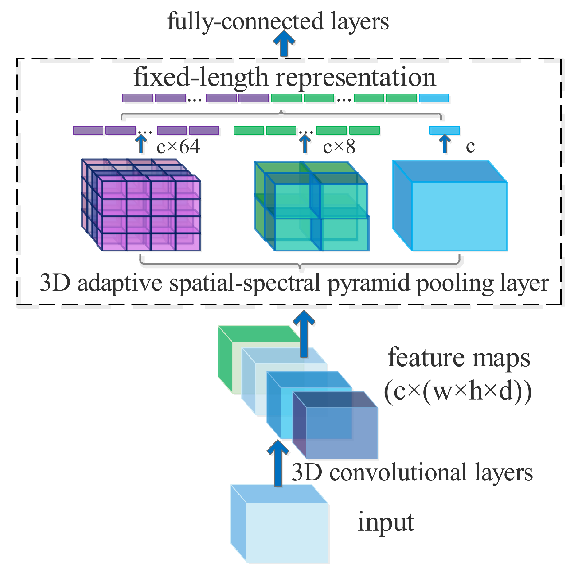
Figure 5.
A CNN structure with 3D adaptive spatial-spectral pyramid pooling (ASSP) layer. Here c is the number of filters in the last convolutional layer. This 3D ASSP contains a three-level pyramid with different scale are , and , respectively.
Figure 5.
A CNN structure with 3D adaptive spatial-spectral pyramid pooling (ASSP) layer. Here c is the number of filters in the last convolutional layer. This 3D ASSP contains a three-level pyramid with different scale are , and , respectively.
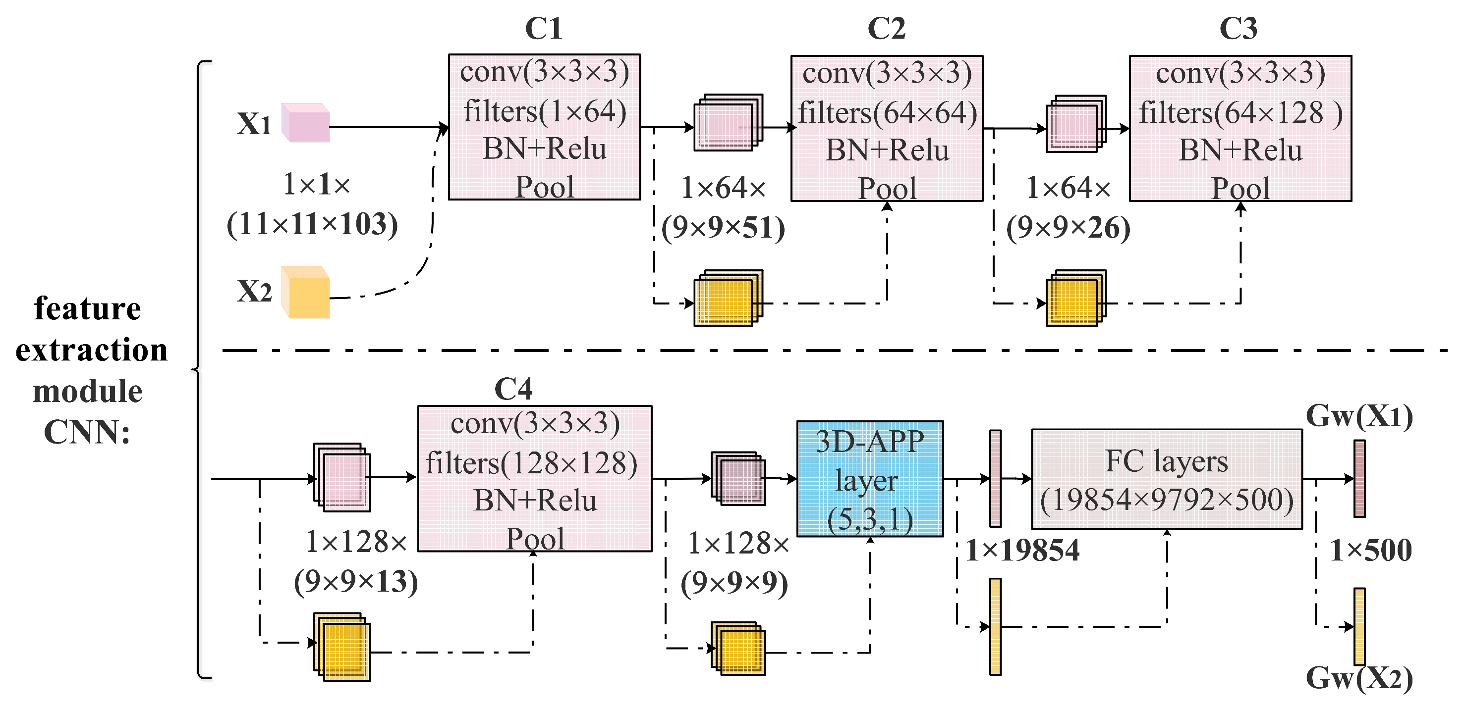
Figure 6.
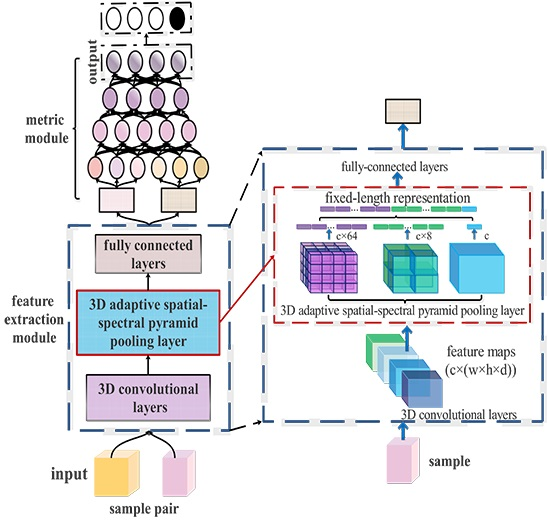
Architecture of our feature extraction with a 3D adaptive spatial-spectral pyramid pooling layer. It contains four 3D CNN blocks, a 3D ASSP layer and three fully connected layers. The input of the feature extraction is a 3D sample-pair and output are two features with the same size.
Figure 6.
Architecture of our feature extraction with a 3D adaptive spatial-spectral pyramid pooling layer. It contains four 3D CNN blocks, a 3D ASSP layer and three fully connected layers. The input of the feature extraction is a 3D sample-pair and output are two features with the same size.
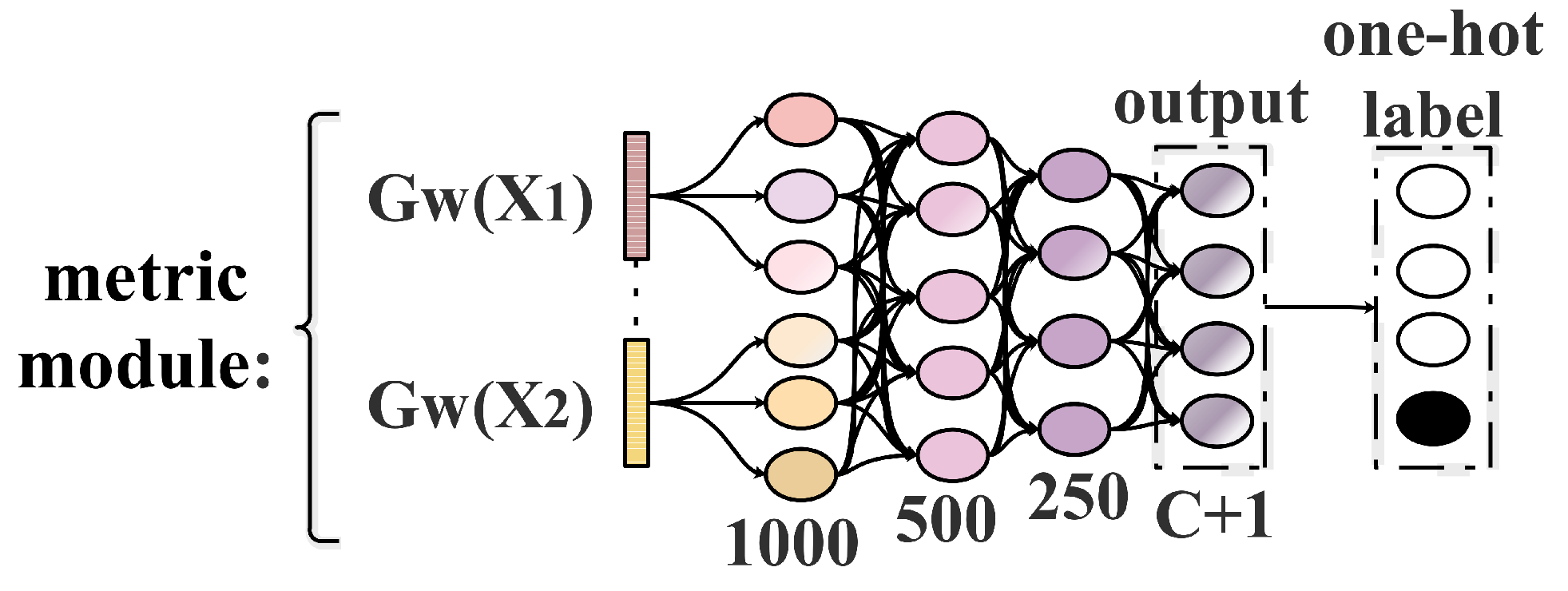
Figure 7.
Architecture of our metric module, which is a fully connected network containing four fully connected layers. The input is the concatenation between a sample-pair’s features and . The output layer contains neuron nodes, where C is the number of classes in HSI.
Figure 7.
Architecture of our metric module, which is a fully connected network containing four fully connected layers. The input is the concatenation between a sample-pair’s features and . The output layer contains neuron nodes, where C is the number of classes in HSI.
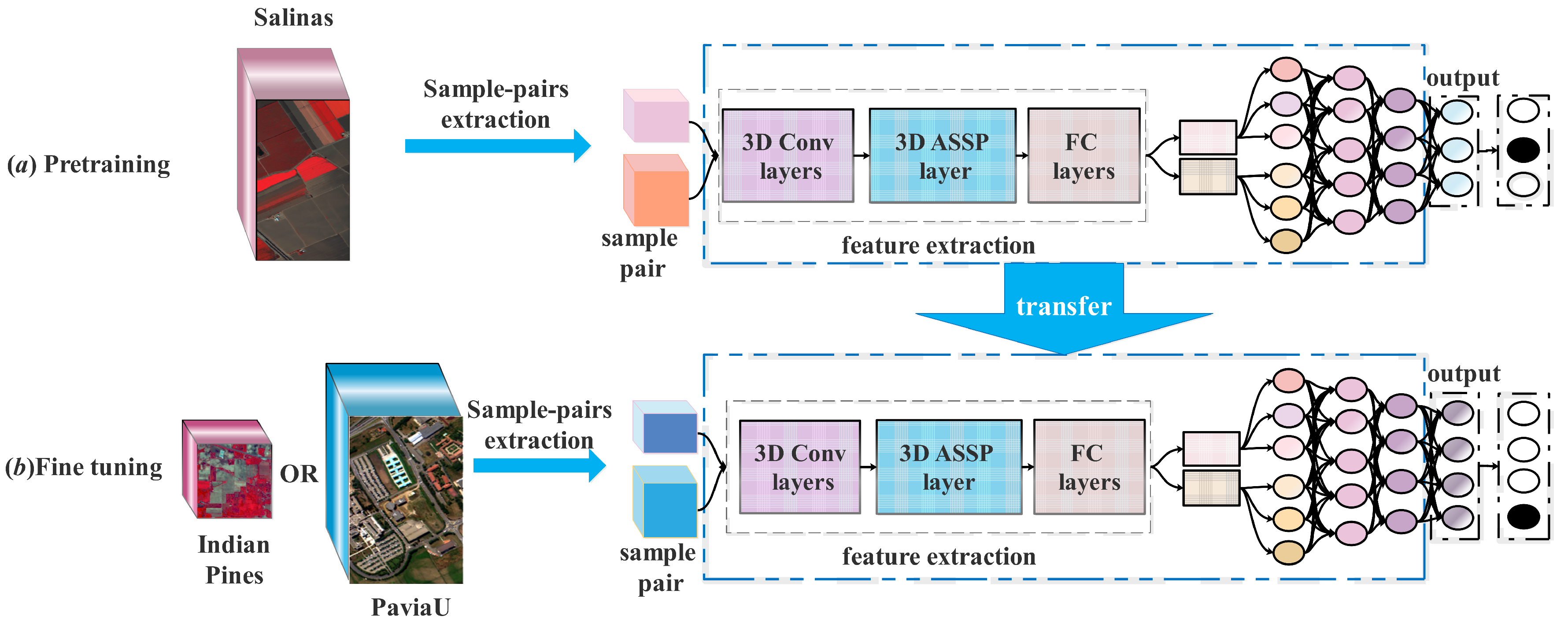
Figure 8.
Transfer learning strategy based on ASSP-SCNN. (a) Pre-training an ASSP-SCNN in source HSI dataset with limited labeled samples. Here the target HSI dataset and source HSI dataset can be collected by the different sensors. (b) Fine-tuning strategy. After ASSP-SCNN is pre-trained, we transfer the entire model except for the output layer to the network built for target HSI dataset as initialization. We then fine-tune the transferred part and the new output layer on target HSI dataset.
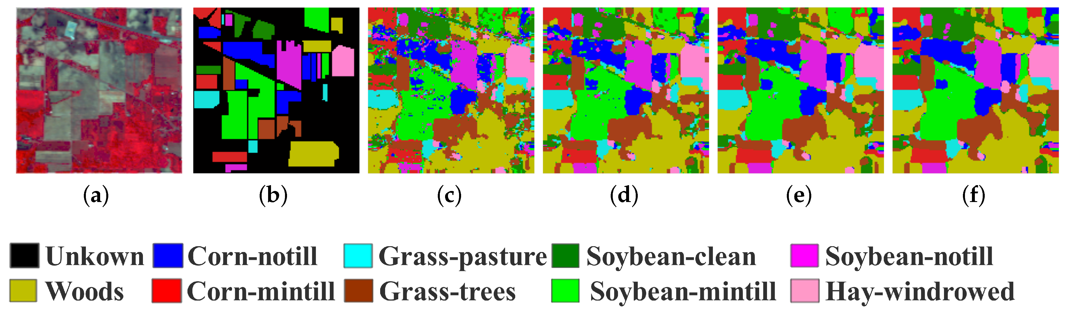
Figure 9.
Thematic maps and OA (%) resulting from the ASSP-SCNN with different spatial window size on Indian Pines dataset with nine classes. (a) Pseudocolor image. (b) Ground-truth map. (c–f) Classification maps with to be , , and , respectively.
Figure 9.
Thematic maps and OA (%) resulting from the ASSP-SCNN with different spatial window size on Indian Pines dataset with nine classes. (a) Pseudocolor image. (b) Ground-truth map. (c–f) Classification maps with to be , , and , respectively.
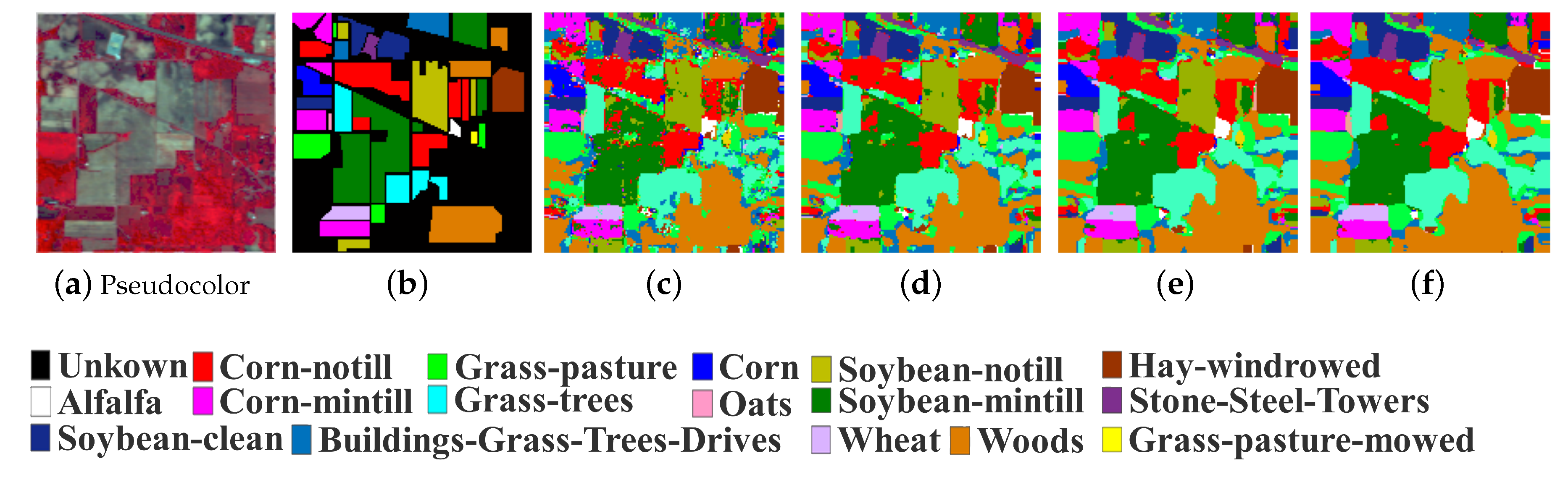
Figure 10.
Thematic maps and OA (%) resulting from the ASSP-SCNN with different spatial window size on Indian Pines dataset with 16 classes. (a) Pseudocolor image. (b) Ground-truth map. (c–f) Classification maps with to be , , and , respectively.
Figure 10.
Thematic maps and OA (%) resulting from the ASSP-SCNN with different spatial window size on Indian Pines dataset with 16 classes. (a) Pseudocolor image. (b) Ground-truth map. (c–f) Classification maps with to be , , and , respectively.
Figure 11.
Thematic maps and OA (%) resulting from the ASSP-SCNN with different spatial window size on PaviaU dataset with nine classes. (a) Pseudocolor image. (b) Ground-truth map. (c–f) Classification maps with to be , , and , respectively.
Figure 11.
Thematic maps and OA (%) resulting from the ASSP-SCNN with different spatial window size on PaviaU dataset with nine classes. (a) Pseudocolor image. (b) Ground-truth map. (c–f) Classification maps with to be , , and , respectively.
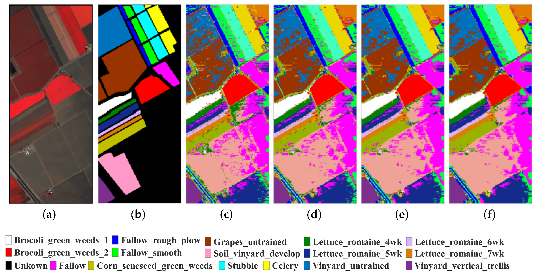
Figure 12.
Thematic maps and OA (%) resulting from the ASSP-SCNN with different spatial window size on Salinas dataset with 16 classes. (a) Pseudocolor image. (b) Ground-truth map. (c–f) Classification maps with to be , , and , respectively.
Figure 12.
Thematic maps and OA (%) resulting from the ASSP-SCNN with different spatial window size on Salinas dataset with 16 classes. (a) Pseudocolor image. (b) Ground-truth map. (c–f) Classification maps with to be , , and , respectively.
Table 1.
Details of the Three Data Sets: Indian Pines, PaviaU, and Salinas.
Table 1.
Details of the Three Data Sets: Indian Pines, PaviaU, and Salinas.
| | Indian Pines | PaiaU | Salinas |
|---|
| Spatial size (pixels) | | | |
| Spectral range (nm) | 400–2500 | 430–860 | 400–2500 |
| Number of bands | 200 | 103 | 204 |
| GSD (m) | 20 | 1.3 | 3.7 |
| Sensor type | AVIRIS | ROSIS | AVIRIS |
| Areas | Indiana | Pavia | California |
| Number of classes | 16 | 9 | 16 |
| Provider | Purdue University | Prof. Paolo Gamba | Jet Propulsion Laboratory |
Table 2.
Statisticsof Training pixels, Validation pixels and Testing pixels for the Indian Pines DataSet.
Table 2.
Statisticsof Training pixels, Validation pixels and Testing pixels for the Indian Pines DataSet.
| No. | Class | Training | Validation | Testing |
|---|
| 1 | Alfalfa | 18 | 4 | 24 |
| 2 | Corn-notill | 180 | 20 | 1228 |
| 3 | Corn-mintill | 180 | 20 | 630 |
| 4 | Corn | 94 | 23 | 120 |
| 5 | Grass-pasture | 180 | 20 | 283 |
| 6 | Grass-trees | 180 | 20 | 530 |
| 7 | Grass-pasture-mowed | 11 | 2 | 15 |
| 8 | Hay-windrowed | 180 | 20 | 278 |
| 9 | Oats | 8 | 2 | 10 |
| 10 | Soybean-notill | 180 | 20 | 772 |
| 11 | Soybean-mintill | 180 | 20 | 2255 |
| 12 | Soybean-clean | 180 | 20 | 393 |
| 13 | Wheat | 82 | 20 | 103 |
| 14 | Woods | 180 | 20 | 1065 |
| 15 | Building-Grass-Trees-Drives | 154 | 38 | 194 |
| 16 | Stone-Steel-Towers | 37 | 9 | 47 |
| Tota | 2024 | 278 | 7947 |
Table 3.
Statistics of Training pixels, Validation pixels and Testing pixels for the PaviaU DataSet.
Table 3.
Statistics of Training pixels, Validation pixels and Testing pixels for the PaviaU DataSet.
| No. | Class | Training | Validation | Testing |
|---|
| 1 | Asphalt | 180 | 20 | 6431 |
| 2 | Meadows | 180 | 20 | 18,449 |
| 3 | Gravel | 180 | 20 | 1899 |
| 4 | Trees | 180 | 20 | 2864 |
| 5 | Sheets | 180 | 20 | 1145 |
| 6 | Bare Soil | 180 | 20 | 4829 |
| 7 | Bitumen | 180 | 20 | 1130 |
| 8 | Bricks | 180 | 20 | 3482 |
| 9 | Shadows | 180 | 20 | 747 |
| Total | 1620 | 180 | 40,976 |
Table 4.
Statistics of Training pixels, Validation pixels and Testing pixels for the Salinas DataSet.
Table 4.
Statistics of Training pixels, Validation pixels and Testing pixels for the Salinas DataSet.
| No. | Class | Training | Validation | Testing |
|---|
| 1 | Broccoli_green_weeds_1 | 180 | 20 | 1809 |
| 2 | Broccoli_green_weeds_2 | 180 | 20 | 3526 |
| 3 | Fallow | 180 | 20 | 1776 |
| 4 | Fallow_rough_plow | 180 | 20 | 1194 |
| 5 | Fallow_smooth | 180 | 20 | 2478 |
| 6 | Stubble | 180 | 20 | 3759 |
| 7 | Celery | 180 | 20 | 3379 |
| 8 | Grapes_untrained | 180 | 20 | 11,071 |
| 9 | Soil_vineyard_develop | 180 | 20 | 6003 |
| 10 | Corn_senesced_green_weeds | 180 | 20 | 3078 |
| 11 | Lettuce_romaine_4wk | 180 | 20 | 868 |
| 12 | Lettuce_romaine_5wk | 180 | 20 | 1727 |
| 13 | Lettuce_romaine_6wk | 180 | 20 | 716 |
| 14 | Lettuce_romaine_7wk | 180 | 20 | 870 |
| 15 | Vineyard_untrained | 180 | 20 | 7068 |
| 16 | Vineyard_vertical_trellis | 180 | 20 | 1607 |
| Total | 2880 | 320 | 50,929 |
Table 5.
The sizes of training sample-pair set, validation sample-pair set and testing sample-pair set for The Three Data Sets: Indian Pines, PaviaU and Salinas. Here the number of spatial window K set to be 4 and the corresponding spatial window size are , , and .
Table 5.
The sizes of training sample-pair set, validation sample-pair set and testing sample-pair set for The Three Data Sets: Indian Pines, PaviaU and Salinas. Here the number of spatial window K set to be 4 and the corresponding spatial window size are , , and .
| | Training Set | Validation Set | Testing Set |
|---|
| Indian Pines | 16,386,304 | 278 | 7947 |
| PaviaU | 10,497,600 | 180 | 40,976 |
| Salinas | 33,177,600 | 320 | 50,929 |
Table 6.
Class-specific accuracy (%), OA (%) and Kappa coefficient generate by the ASSP-SCNNs on PaviaU dataset. Here we equip ASSP-SCNN with seven different ASSP layer with size and , respectively.
Table 6.
Class-specific accuracy (%), OA (%) and Kappa coefficient generate by the ASSP-SCNNs on PaviaU dataset. Here we equip ASSP-SCNN with seven different ASSP layer with size and , respectively.
| No. | | | | | | | |
|---|
| 1 | 98.63 | 97.30 | 97.95 | 95.48 | 97.13 | 97.67 | 99.02 |
| 2 | 98.95 | 99.51 | 99.37 | 99.61 | 99.76 | 99.77 | 99.84 |
| 3 | 93.79 | 97.49 | 96.56 | 92.84 | 96.19 | 94.88 | 95.05 |
| 4 | 96.05 | 97.10 | 97.15 | 97.61 | 98.89 | 98.69 | 98.86 |
| 5 | 97.65 | 99.96 | 99.83 | 99.18 | 99.26 | 99.13 | 99.96 |
| 6 | 97.12 | 99.01 | 99.53 | 99.32 | 99.41 | 98.92 | 99.49 |
| 7 | 93.56 | 89.84 | 91.30 | 83.75 | 89.93 | 90.60 | 98.11 |
| 8 | 97.50 | 97.30 | 98.03 | 95.37 | 98.21 | 95.50 | 96.66 |
| 9 | 98.53 | 95.10 | 97.26 | 95.09 | 96.88 | 98.16 | 99.14 |
| OA | 97.906 | 98.289 | 98.504 | 97.511 | 98.582 | 98.358 | 99.048 |
| Kappa | 0.972 | 0.977 | 0.980 | 0.967 | 0.981 | 0.978 | 0.987 |
Table 7.
Class-specific accuracies (%), OA (%) and Kappa coefficients generate by the ASSP-SCNNs on PaviaU dataset. Here we train the ASSP-SCNN by a constructing 3D sample-pair set according to different spatial window size combinations and , respectively.
Table 7.
Class-specific accuracies (%), OA (%) and Kappa coefficients generate by the ASSP-SCNNs on PaviaU dataset. Here we train the ASSP-SCNN by a constructing 3D sample-pair set according to different spatial window size combinations and , respectively.
| No. | 7 | 9 | 11 | 13 | 15 | | | |
|---|
| 1 | 97.95 | 98.00 | 99.02 | 98.31 | 98.03 | 99.34 | 99.60 | 99.10 |
| 2 | 98.90 | 99.31 | 99.84 | 99.46 | 99.18 | 99.43 | 99.69 | 99.87 |
| 3 | 95.62 | 96.49 | 95.05 | 97.49 | 96.53 | 98.76 | 97.75 | 99.55 |
| 4 | 95.29 | 99.18 | 98.86 | 96.84 | 95.65 | 97.58 | 98.52 | 99.39 |
| 5 | 99.83 | 99.44 | 99.96 | 99.39 | 98.54 | 99.96 | 99.83 | 100.00 |
| 6 | 98.09 | 97.63 | 99.49 | 98.96 | 99.09 | 98.68 | 99.23 | 99.47 |
| 7 | 94.96 | 93.43 | 98.11 | 96.98 | 96.76 | 97.47 | 98.81 | 97.39 |
| 8 | 96.17 | 97.18 | 96.66 | 97.55 | 98.06 | 98.91 | 98.48 | 99.51 |
| 9 | 94.62 | 94.44 | 99.14 | 93.55 | 95.46 | 97.84 | 96.70 | 97.45 |
| OA | 97.840 | 98.323 | 99.048 | 98.592 | 98.358 | 99.051 | 99.268 | 99.512 |
| Kappa | 0.971 | 0.978 | 0.987 | 0.981 | 0.978 | 0.987 | 0.990 | 0.993 |
Table 8.
Class-specific accuracy (%), OA (%) and Kappa coefficient of ASSP-SCNN and the comparing methods on Indian Pines dataset with nine classes.
Table 8.
Class-specific accuracy (%), OA (%) and Kappa coefficient of ASSP-SCNN and the comparing methods on Indian Pines dataset with nine classes.
| No. | SVM-RFS | 1D-CNN | CNN-PPF | C-CNN | SVM+SCNN | DFSL+SVM | ASSP-SCNN |
|---|
| 2 | 88.73 | 79.63 | 92.99 | 96.28 | 98.25 | 98.32 | 99.27 |
| 3 | 91.20 | 69.48 | 96.66 | 92.26 | 99.64 | 99.76 | 98.44 |
| 5 | 97.52 | 85.80 | 98.58 | 99.30 | 97.10 | 100.00 | 99.65 |
| 6 | 99.86 | 94.95 | 100.00 | 99.25 | 99.86 | 100.00 | 99.72 |
| 8 | 100.00 | 98.57 | 100.00 | 100.00 | 100.00 | 100.00 | 100.00 |
| 10 | 91.67 | 71.41 | 96.24 | 92.84 | 98.87 | 97.84 | 99.29 |
| 11 | 78.79 | 90.44 | 87.80 | 98.21 | 98.57 | 95.93 | 98.77 |
| 12 | 93.76 | 72.26 | 98.98 | 92.45 | 100.00 | 99.66 | 98.62 |
| 14 | 98.74 | 99.90 | 99.81 | 98.98 | 100.00 | 99.76 | 99.81 |
| OA | 89.83 | 84.44 | 94.34 | 96.76 | 99.04 | 98.35 | 99.17 |
| Kappa | 0.871 | 0.825 | 0.947 | 0.959 | 0.989 | 0.981 | 0.990 |
Table 9.
Class-specific accuracy (%), OA (%) and Kappa coefficient of ASSP-SCNN and the comparing methods on PaviaU dataset with nine classes.
Table 9.
Class-specific accuracy (%), OA (%) and Kappa coefficient of ASSP-SCNN and the comparing methods on PaviaU dataset with nine classes.
| No. | SVM-RFS | dgcForest | 1D-CNN | CNN-PPF | C-CNN | SVM+SCNN | DFSL+SVM | ASSP-SCNN |
|---|
| 1 | 87.95 | 92.92 | 85.62 | 97.42 | 97.40 | 98.69 | 97.18 | 99.13 |
| 2 | 97.17 | 96.88 | 88.92 | 95.76 | 99.40 | 99.58 | 99.40 | 99.95 |
| 3 | 86.99 | 74.31 | 80.51 | 94.52 | 94.48 | 99.52 | 97.90 | 98.44 |
| 4 | 95.50 | 90.79 | 96.93 | 97.52 | 99.16 | 99.22 | 98.40 | 99.46 |
| 5 | 99.85 | 98.90 | 99.30 | 100.00 | 100.00 | 100.00 | 100.00 | 99.83 |
| 6 | 94.31 | 78.60 | 84.30 | 99.13 | 98.70 | 98.85 | 99.56 | 99.91 |
| 7 | 94.74 | 78.76 | 92.39 | 96.19 | 100.00 | 99.32 | 99.25 | 96.87 |
| 8 | 85.89 | 87.69 | 80.73 | 93.62 | 94.57 | 96.58 | 95.52 | 98.87 |
| 9 | 99.89 | 99.85 | 99.20 | 99.87 | 99.87 | 100.00 | 99.68 | 99.34 |
| OA | 91.10 | 91.35 | 87.90 | 96.48 | 98.41 | 99.08 | 98.62 | 99.52 |
| Kappa | 0.882 | 0.884 | 0.838 | 0.951 | 0.979 | 0.988 | 0.982 | 0.993 |
Table 10.
Class-specific accuracy (%), OA (%) and Kappa coefficient of ASSP-SCNN and the comparing methods on Salinas dataset with sixteen classes.
Table 10.
Class-specific accuracy (%), OA (%) and Kappa coefficient of ASSP-SCNN and the comparing methods on Salinas dataset with sixteen classes.
| No. | SVM-RFS | dgcForest | 1D-CNN | CNN-PPF | C-CNN | DFSL+SVM | ASSP-SCNN |
|---|
| 1 | 99.55 | 99.48 | 98.73 | 100.00 | 100.00 | 100.00 | 99.97 |
| 2 | 99.92 | 99.81 | 99.12 | .88 | 99.89 | 99.97 | 99.99 |
| 3 | 99.44 | 99.10 | 96.08 | 99.60 | 99.89 | 100.00 | 99.97 |
| 4 | 99.86 | 99.38 | 99.71 | 99.49 | 99.25 | 99.86 | 99.83 |
| 5 | 98.02 | 97.92 | 97.04 | 98.34 | 99.39 | 100.00 | 99.94 |
| 6 | 99.70 | 99.74 | 99.59 | 99.97 | 100.00 | 100.00 | 99.99 |
| 7 | 99.69 | 99.32 | 99.33 | 100.00 | 99.82 | 100.00 | 99.84 |
| 8 | 84.85 | 87.71 | 78.64 | 88.68 | 91.45 | 91.67 | 95.95 |
| 9 | 99.58 | 99.42 | 98.04 | 98.33 | 99.95 | 99.69 | 99.99 |
| 10 | 96.49 | 93.20 | 92.38 | 98.60 | 98.51 | 99.79 | 98.90 |
| 11 | 98.78 | 96.06 | 99.14 | 99.54 | 99.31 | 100.00 | 98.52 |
| 12 | 100.00 | 99.30 | 99.88 | 100.00 | 100.00 | 100.00 | 99.94 |
| 13 | 99.13 | 98.22 | 97.84 | 99.44 | 99.72 | 100.00 | 99.86 |
| 14 | 98.97 | 92.40 | 96.17 | 98.96 | 100.00 | 100.00 | 98.36 |
| 15 | 76.38 | 68.05 | 72.69 | 83.53 | 96.24 | 97.01 | 94.16 |
| 16 | 99.56 | 97.80 | 98.59 | 99.31 | 99.63 | 99.94 | 99.44 |
| OA | 93.15 | 92.07 | 90.25 | 94.80 | 97.42 | 97.81 | 98.15 |
| Kappa | 0.923 | 0.912 | 0.895 | 0.938 | 0.971 | 0.976 | 0.979 |
Table 11.
Class-specific accuracy (%), OA (%) and Kappa coefficient of ASSP-SCNN on Indian Pines dataset with sixteen classes.
Table 11.
Class-specific accuracy (%), OA (%) and Kappa coefficient of ASSP-SCNN on Indian Pines dataset with sixteen classes.
| Class No. | Training Number | Class-Specific Accuracy | Class No. | Training Number | Class-Specific Accuracy |
|---|
| 1 | 18 | 97.96 | 9 | 8 | 90.91 |
| 2 | 180 | 95.88 | 10 | 180 | 96.56 |
| 3 | 180 | 98.50 | 11 | 180 | 97.31 |
| 4 | 94 | 98.74 | 12 | 180 | 596.54 |
| 5 | 180 | 99.82 | 13 | 82 | 100.00 |
| 6 | 180 | 99.91 | 14 | 180 | 99.76 |
| 7 | 11 | 100.00 | 15 | 154 | 98.48 |
| 8 | 180 | 100.00 | 16 | 37 | 98.95 |
| OA | 97.848 | Kappa | 0.975 |
Table 12.
OA (%) generated by the ASSP-SCNN-based transfer learning framework between the three HSI datasets.
Table 12.
OA (%) generated by the ASSP-SCNN-based transfer learning framework between the three HSI datasets.
| Source Dataset | Number of Labeled Pixels per Class for Fine-Tuning | Target Dataset |
|---|
| 25 | 50 | 100 | 150 | 200 |
|---|
| Indian Pines_9 | 93.648 | 97.138 | 98.055 | 98.788 | 99.132 | Indian Pines_16 |
| 93.925 | 96.458 | 99.011 | 99.237 | 99.549 | PaviaU |
| 92.900 | 93.865 | 96.512 | 97.470 | 97.997 | Salinas |
| Indian Pines_16 | 98.213 | 98.156 | 97.840 | 99.137 | 99.475 | Indian Pines_9 |
| 92.247 | 96.156 | 98.543 | 99.353 | 99.614 | PaviaU |
| 92.849 | 94.408 | 96.754 | 97.854 | 98.315 | Salinas |
| PaviaU | 83.716 | 94.410 | 96.460 | 98.034 | 98.803 | Indian Pines_9 |
| 79.397 | 89.128 | 95.733 | 97.353 | 98.425 | Indian Pines_16 |
| 92.682 | 93.833 | 96.954 | 97.823 | 98.209 | Salinas |
| Salinas | 83.494 | 91.337 | 96.472 | 98.300 | 98.709 | Indian Pines_9 |
| 73.015 | 88.345 | 95.199 | 97.423 | 98.226 | Indian Pines_16 |
| 93.833 | 95.289 | 98.450 | 99.331 | 99.492 | PaviaU |
Table 13.
Time (hour) for training ASSP-SCNN without pre-training or fine-tuning the pre-trained ASSP-SCNN on three HSI target datasets.
Table 13.
Time (hour) for training ASSP-SCNN without pre-training or fine-tuning the pre-trained ASSP-SCNN on three HSI target datasets.
| Target Dataset | Without | Pre-Training on | Pre-Training on | Pre-Training on | Pre-Training on |
|---|
| Pre-Training | Indian Pines_9 | Indian Pines_16 | PaviaU | Salinas |
|---|
| Indian Pines_9 (>98.6%) | 2.7 | / | 0.4 | 3.3 | 6.9 |
| Indian Pines_16 (>97.5%) | 9.5 | 0.4 | / | 8.0 | 10.7 |
| PaviaU (>99.4%) | 7.1 | 5.4 | 5.5 | / | 2.8 |
| Salinas (>97.9%) | 14.9 | 6.8 | 5.2 | 2.6 | / |


